Abstract
Accurate wind-speed prediction plays an important role in improving the operation stability of wind-power generation systems. However, the inherent complexity of meteorological dynamics poses a major challenge to forecasting accuracy. In order to overcome these limitations, we propose a new hybrid framework, which combines variational mode decomposition (VMD) for signal processing, enhanced quantum particle swarm optimization (e-QPSO), an improved walking optimization algorithm (IHOA) for feature selection and the long short-term memory (LSTM) network, and which finally establishes a reliable prediction architecture. The purpose of this paper is to optimize VMD by using the e-QPSO algorithm to improve the problems of excessive filtering or error filtering caused by parameter problems in VMD, as the noise signal cannot be filtered completely, and the number of sources cannot be accurately estimated. The IHOA algorithm is used to find the optimal hyperparameters of LSTM to improve the learning efficiency of neurons and improve the fitting ability of the model. The proposed e-QPSO-VMD-IHOA-LSTM model is compared with six established benchmark models to verify its predictive ability. The effectiveness of the model is verified by experiments using the hourly wind-speed data measured in four seasons in Changchun in 2023. The MAPE values of the four datasets were 0.0460, 0.0212, 0.0263, and 0.0371, respectively. The results show that e-QPSO-VMD effectively processes the data and avoids the problem of error filtering, while IHOA effectively optimizes the LSTM parameters and improves prediction performance.
1. Introduction
The environmental and operational limitations of conventional fossil energy systems have become increasingly apparent as global energy demands escalate. In contrast to these traditional sources associated with ecological degradation [], renewable alternatives such as wind energy demonstrate superior sustainability and environmental compatibility. Wind-power generation represents a promising solution to addressing energy supply constraints while reducing anthropogenic pollution [,].
Nevertheless, the stochastic and nonlinear nature of wind-speed patterns creates substantial technical barriers for grid-integrated wind-power systems. This inherent meteorological variability induces generation intermittency, resulting in
- (1)
- Operational instabilities threatening grid reliability, requiring the implementation of advanced management protocols, energy storage systems, and adaptive contingency strategies;
- (2)
- Increased complexity in resource forecasting and infrastructure planning for power-system operators and renewable-energy developers.
The key to addressing these issues lies in developing accurate wind-speed prediction methods, which are crucial for resolving related challenges [,]. Technologies capable of accurately predicting wind speeds can provide a foundation for power dispatch and planning activities, helping to balance supply and demand in power grids. Their significance lies in reducing the negative impacts of supply–demand imbalances on grids, thereby extending the operational lifespan of grid connections [].
Wind-speed forecasting is conventionally classified into four temporal categories according to prediction horizons []:
- Ultra-short-term (minutes to 30 min) [,];
- Short-term (30 min–6 h) [,];
- Medium-term (6–24 h) [,];
- Long-term (>24 h) [,].
These forecasting horizons fulfill distinct operational functions: ultra-short-term forecasts enable real-time turbine regulation and generation compliance monitoring; short-term predictions optimize load-dispatching strategies; medium-term projections enhance grid operational management; whereas long-term forecasts inform maintenance scheduling and infrastructure planning [].
Current research in wind-power forecasting primarily follows two directions. The first approach directly predicts future power generation using wind-power data or numerical weather-prediction data, known as the direct method. The alternative indirect approach adopts a two-stage process: initially establishing a wind-power curve prediction model, followed by wind-speed prediction. The forecasted wind speeds are then input into this model to derive the final power-generation estimates [,]. This research focuses on wind-speed forecasting within the indirect modeling framework, where methodologies are divided into two principal categories: physics-based numerical models and data-driven machine-learning techniques. Physical approaches leverage fluid dynamics and thermodynamic principles to systematically integrate atmospheric boundary layer parameters, ocean-atmosphere thermal exchange mechanisms, and topographic terrain effects, forming a cohesive simulation system for meteorological interactions []. However, these approaches often encounter implementation challenges and computational complexity, rendering them more suitable for medium-to-long-term forecasting applications. Machine-learning approaches in wind forecasting predominantly utilize Numerical Weather Prediction (NWP) datasets incorporating wind speed/direction, temperature profiles, and historical wind-pattern analytics to develop predictive systems []. Contemporary temporal forecasting architectures feature three prominent neural-network variants: Recurrent Neural Networks (RNNs) for sequential pattern extraction [], Long Short-Term Memory (LSTM) networks addressing temporal dependencies [], and Graph Neural Networks (GNNs) handling spatial correlations [], each demonstrating unique advantages in meteorological time-series modeling. As research advances and datasets grow increasingly complex, the inherent limitations of individual algorithms across diverse data environments have become more apparent. In response to these challenges, researchers have developed hybrid machine-learning frameworks that synergistically combine multiple models to enhance predictive accuracy. Comparative studies have demonstrated the superior performance of such ensemble approaches over singular models in wind-speed forecasting applications []. This integrated methodology capitalizes on the complementary strengths of constituent models while mitigating their respective weaknesses.
A fundamental challenge in wind-speed prediction stems from the intrinsic properties of raw meteorological signals, which demonstrate pronounced noise contamination, discrete sampling artifacts, and non-stationary behavior that traditional statistical approaches often fail to adequately process. To mitigate these constraints, advanced decomposition techniques including Empirical Wavelet Transform (EWT), Empirical Mode Decomposition (EMD), and their enhanced variants like Ensemble EMD (EEMD) have been increasingly adopted for data preconditioning. In tackling wind-speed time-series nonlinearity, Liu et al. [] pioneered an integrated framework coupling EWT with LSTM-ELMAN neural topologies, achieving enhanced prediction robustness through multi-scale feature disentanglement, while Tian et al. [] proposed a short-term prediction framework utilizing EEMD and RARIMA (Recursive Autoregressive Integrated Moving Average) models. Li et al. [] implemented the Complete Ensemble Empirical Mode Decomposition with the Adaptive Noise (CEEMDAN) technique to decompose and reconstruct raw wind-speed sequences, thereby mitigating volatility and randomness. Hu et al. [] proposed a hybrid forecasting framework synergistically integrating Variational Mode Decomposition (VMD), Differential Evolution (DE) optimization, and Echo State Networks (ESN), establishing an enhanced prediction architecture with improved stability in fluctuating wind regimes. However, this approach raises concerns about potential over-decomposition and an insufficient rationale for controlling VMD decomposition layers, which may lead to excessive computational-resource consumption.
Nevertheless, traditional independent models and decomposition methods lack optimization mechanisms, and have serious operational limitations in meeting the accuracy requirements of modern power-grid dispatching systems. In order to make up for this technical gap, we propose an innovative e-QPSO-VMD-IHOA-LSTM hybrid framework. Based on the hybrid prediction architecture, the framework collaboratively integrates enhanced quantum particle swarm optimization (e-QPSO), variational mode decomposition (VMD), the improved walking optimization algorithm (IHOA), and the long short-term memory (LSTM) network. Compared with the previous research, the contribution of this study is to optimize VMD by using the e-QPSO algorithm to avoid the poor decomposition effect of VMD caused by the manual parameter adjustment, and to optimize the LSTM parameters by using the IHOA optimization algorithm to achieve a better fitting effect. There are three main innovations in this study:
- This study proposes a new e-QPSO-VMD-IHOA-LSTM hybrid wind-speed prediction model. Compared with manual tuning and the popular WOA algorithm [] to optimize VMD, the e-QPSO algorithm has a better optimization ability, effectively solves the problem of modal mixing and incomplete decomposition, and improves decomposition efficiency;
- An improved walking optimization algorithm (IHOA) is proposed by combining the Tent chaotic map with the quantum particle swarm optimization (QPSO) strategy and stochastic differential mutation. Tent mapping enhances the initial population diversity and solution quality. QPSO integration enhances the population exploration ability and global search performance. The stochastic differential mutation mechanism reduces the local optimal capture and improves convergence accuracy. Through the improvement of three strategies, the applicability of the algorithm is effectively improved;
- By using the e-QPSO algorithm to optimize VMD, the purpose of this method is to find several signals with center frequency and a certain bandwidth of wind-speed signal, so as to reduce the influence of noise on wind speed, and each demodulated component is relatively smooth and easier to learn. IHOA is used to optimize the three key parameters of LSTM: maximum hidden layer size, training iteration, and learning rate to further enhance the learning ability of the model and improve the prediction accuracy. The key of the model proposed in this paper is to realize the data preprocessing stage to retain the statistical characteristics of the sequence, reduce the influence of noise on training, and the parameter optimization stage to enhance the training efficiency through the optimization of LSTM hyperparameters.
2. Methods
2.1. Variational Mode Decomposition
The VMD method, proposed by Yanovsky, I.; Dragomiretskiy, K., et al. [] in 2014, is a signal-decomposition technique that decomposes an original signal f(t) into multiple Intrinsic Mode Functions (IMFs) with distinct central frequencies and bandwidths. This approach enforces constraints to ensure that each mode exhibits limited bandwidth and a specific central frequency. The variational model is formulated as follows:
The original signal is denoted by . To address scenarios involving Gaussian noise interference, we introduced a Lagrangian multiplier and a penalty coefficient . This formulation employs a strategic transformation of constraints, converting the constrained variational problem into an unconstrained optimization framework. The modified formulation serves dual purposes: it simplifies the solution process while simultaneously mitigating the impact of noise contamination. The complete mathematical expression can be written as
By integrating the Fourier isometric transformation with the Alternating Direction Penalty Algorithm (ADMM), the iterative update expressions for , , and are derived through alternating optimization as follows:
The parameter denotes the noise tolerance threshold that ensures decomposition fidelity requirements. The Fourier transform of corresponds to the Wiener filtering component for . In variational mode decomposition (VMD), the penalty coefficient α and the number of intrinsic mode functions (IMFs) K critically influence signal-decomposition performance. The parameter descriptions of Equations (1)–(5) are shown in Table 1.

Table 1.
The description of the parameters in Equations (1)–(5).
The parameter K determines the quantity of IMFs generated during signal decomposition. An excessively large K may induce over-decomposition with spurious components, while an insufficient K could result in under-decomposition that fails to adequately extract critical signal constituents. The penalty coefficient α regulates the trade-off between reconstruction error and the bandwidth constraints of modal components. A higher α value enforces narrower bandwidths for IMFs, effectively mitigating mode mixing at the potential cost of localized information loss. Conversely, a lower α value increases susceptibility to mode mixing, which may compromise feature-extraction accuracy. Proper parameter selection ( and K) is therefore essential for achieving an optimal balance between decomposition resolution and the physical interpretability of the extracted components.
2.2. VMD by e-QPSO
The e-QPSO, proposed by Agrawal, R.K. et al. [], was developed to address the limitation of meta-heuristic algorithms in escaping local optima when solving complex functions due to insufficient exploration capabilities. The enhanced quantum particle swarm optimization (e-QPSO) algorithm incorporates pivotal innovations to refine the exploration–exploitation trade-off inherent in conventional QPSO methodologies. Central to this advancement is the implementation of a dynamically modulated equilibrium mechanism governed by parameter α, which intelligently adjusts the convergence trajectory through the real-time calibration of personal best (pbest) and global best (gbest) position vectors during iterative search processes, a dynamic equilibrium between dispersion and intensification via parameter γ, and the periodic reinitialization of a certain percentage of underperforming population segments to help escape from local optima. These enhancements give e-QPSO superior optimization performance, making it especially suitable for optimizing Variational Mode Decomposition (VMD) parameters.
Sample Entropy (SE) was used to quantify the complexity of the signal. The higher the SE value means the greater the signal complexity, the more noise interference, and the higher the sequence uncertainty, while the lower the SE value means the lower the complexity, the less noise pollution, and the better the sequence predictability. Therefore, the objective of VMD optimization is to minimize the sample entropy of the data, and the mathematical representation of SE as the objective function is shown in Equation (6).
A schematic diagram of e-QPSO optimizing VMD is shown in Figure 1.
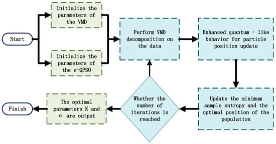
Figure 1.
Flowchart of VMD by e-QPSO.
2.3. Hiking Optimization Algorithm
The HOA [] derives its theoretical foundation from mountaineering dynamics, establishing a direct analogy between optimization search spaces and topographical landscapes. At its core lies Tobler’s Hiking Function (THF), a geospatial model that mathematically formalizes hiker navigation strategies by correlating terrain gradients (elevation/distance ratios) with velocity modulation. During iterative optimization, THF governs agent mobility through the solution space via the velocity–distance relationship:
In Equation (7), is the velocity of hiker i at iteration/time step t (km/h), and in addition, the calculation formula of the slope .
In Equation (8), dh and dt represent the height difference and distance that the hiker passes. In addition, the range is between [0, 50°]. The Hiking Optimization Algorithm (HOA) emulates the collective social dynamics and individual cognitive capabilities of hikers. The updated velocity of each hiker is governed by four factors: initial velocity (determined by the Terrain Hiking Factor, THF), the leading hiker’s position, the hiker’s current position, and a sweep factor. The velocity and position updates for the i-th hiker at iteration are formulated as follows:
In Equation (9), represents a random number in the interval [0, 1]; and denote the current speed and initial speed of the hiker, respectively. and represent the location of the leading hiker and the location of the i-th hiker, and is the sweep factor (SF) of the hiker, which is between [1, 3]. The sweep factor ensures that the hikers will not deviate too far from the lead hikers so that they can see the direction of the lead hikers and receive signals from the lead hikers. In Equation (10), is the current position of the i-th hiker. The parameter descriptions of Equations (7)–(10) are shown in Table 2.
Table 2.
The description of the parameters in Equations (7)–(10).
2.4. Improvements to Hiking Optimization Algorithm
(1): The Tent chaotic map was used to improve the initialization. The population initialization of the standard walking optimization algorithm (HOA) was performed by random generation. This method has many shortcomings, including the uneven distribution of hikers, weak global exploration, low population diversity, and susceptibility to local optima. To address these limitations, we integrated chaotic maps, which blend deterministic behavior with stochastic randomness, offering aperiodicity and enhanced traversal of the search space. Chaotic initialization has been demonstrated to improve the exploration capabilities of optimization algorithms by generating diverse, well-distributed initial populations, thereby mitigating premature convergence []. Among chaotic maps, the Tent map is particularly effective due to its simplicity and uniform ergodicity. The Tent map is defined as
The upper and lower bounds are ∈ (0,1), and takes 0.5. The distribution of the chaotic sequence of the Tent map is shown in Figure 2. In Figure 2a, the scatter plot shows that the initial points are evenly distributed in each dimension. The histogram in Figure 2b shows the frequency distribution of the initial points. It can be seen that the Tent map is evenly and randomly distributed in the upper and lower limits. The use of Tent mapping can ensure that the initial points are evenly distributed within the unit interval and can ensure that the second half of the generated sequence does not overlap. The quality and diversity of the initial population were improved. The parameter descriptions of Equation (11) are shown in Table 3.
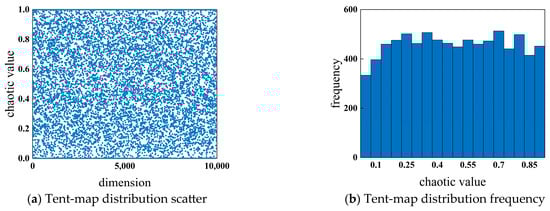
Figure 2.
Tent-mapping distribution.
Table 3.
The description of the parameters in Equation (11).
(2): By introducing the parameters of , , and in QPSO [], the global search ability of the HOA population is enhanced to avoid the population falling into a local optimal solution. In Equation (13), the location is updated by fusing QPSO as shown below. The random number n ∈ (0, 1) is used to determine which formula is selected to update the position of the hiker . When n ≤ 0.5, the position is updated by Equation (15). When n > 0.5, the position is updated by Equation (16). By integrating the QPSO algorithm, the global search ability of the algorithm is enhanced.
By introducing this improved quantum behavior mechanism, the randomness in the HOA position update strategy can be significantly enhanced, and the problem of the original algorithm being prone to falling into a local optimum can be solved. The original HOA has insufficient development around the hikers. Through the new mechanism, the hikers are allowed to search within a certain range of each individual position, which effectively expands the search space. It is beneficial to gradually converge on the same optimal solution, that is, the objective function value, thus enhancing the global optimization ability of the algorithm. The parameter descriptions of Equations (12)–(16) are shown in Table 4.
Table 4.
The description of the parameters in Equations (12)–(16).
(3): The position update mechanism in the original Hiking Optimization Algorithm (HOA) relies heavily on the current optimal individual’s state, which risks premature convergence and reduced population diversity. This overemphasis on leader-following behavior restricts exploration, causing the population to cluster around suboptimal regions and lowering convergence precision. Specifically, in each iteration, the first 70% of the hikers use Equation (15) or Equation (16) to update their position, and the last 30% of the hikers use a random mutation strategy to update it, so as to improve the population diversity of the hikers. The location update method is shown in Equation (17). The parameter descriptions of Equation (17) are shown in Table 5
Table 5.
The description of the parameters in Equation (17).
Equation (17) utilizes random mutation strategies applied to both the leader position and the random walker position. This dual approach not only enhances algorithmic convergence precision but also accelerates the overall convergence process.
To validate the optimization capability and convergence of the Improved Hiking Optimization Algorithm (IHOA), comparative experiments were conducted against the PSO, BBO, ACO, GWO, and original HOA algorithms using the first 12 functions (6 unimodal, 6 multimodal) from the CEC2005 test suite. Each function was tested for over 30 independent runs with a population size of 30 and 1000 iterations, using the mean and standard deviation as performance metrics. Unimodal functions evaluated optimization precision and convergence speed, while multimodal functions assessed the global search ability and local optima avoidance. The test function formulations are provided in Table 6, with results summarized in Table 7 and visualized in Figure 3.
Table 6.
Test function.
Table 7.
Friedman test results on test functions.
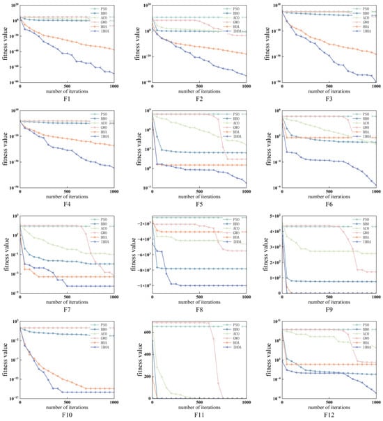
Figure 3.
Convergence curves of different algorithms using the test function.
It can be seen from Figure 3 that among the 12 test functions, F1–F4 can be found to show that IHOA searches at a faster search speed. In functions F5–F7, IHOA does not converge as early as HOA, but still keeps searching in the middle and late stages of iteration, and does not fall into the local optimal solution. In functions F8, F9, F11, and F12, it can be found that the initialization improvement makes the IHOA search to the minimum faster than HOA. In the comparison of 12 functions, compared with the original HOA, IHOA demonstrates superior optimization performance, high precision, and rapid convergence speed and good stability.
In addition, in order to reduce the error caused by randomness, the average value (Avg) and variance (Std) of 30 operation results are used as indicators in Table 6, which can better reflect the solving ability of the algorithm. It can be seen from Table 7 that IHOA has strong global search ability and the ability to quickly escape from local optimal solutions. In the solution of functions F9~F11, the variance is 0, and in other functions, the variance is also smaller than the variance of HOA solution, which indicates that IHOA is superior to the HOA algorithm in terms of stability.
2.5. Long and Short-Term Memory Neural Network (LSTM)
The LSTM, introduced by Hochreiter and Schmidhuber in 1997, which solves the problem of ‘gradient disappearance’ of ordinary RNNs when dealing with long sequences by introducing ‘memory units’. When dealing with long-distance dependencies, the LSTM addresses the issues of vanishing and exploding gradients commonly encountered in standard RNNs by incorporating a gating mechanism, which can effectively remember and transmit information over a long time. The structure diagram is shown in Figure 4. Its mathematical expression is as depicted in Equation (18). The parameter descriptions of Formula (18) are shown in Table 8.
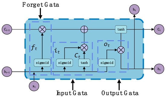
Figure 4.
Schematic diagram of LSTM network model structure.
Table 8.
The description of the parameters in Equation (18).
2.6. e-QPSO-VMD-IHOA-LSTM Model
The specific process is as follows:
- (1)
- The e-QPSO-VMD algorithm decomposes raw wind-speed data into multiple frequency-distinct subsequences. These decomposed components, along with the original dataset, subsequently serve as inputs for wind-speed prediction modeling. The integrated data structure is systematically partitioned into the training and testing subset;
- (2)
- IHOA algorithm parameter initialization coding;
- (3)
- The RMSE minimization is selected as the objective function, and the IHOA algorithm is used to find the optimal maximum number of hidden layers, maximum training iterations, and learning rate of LSTM. The influence of these three parameters on the performance of the LSTM model will be discussed in detail in the next section, based on the actual wind-speed and prediction results;
- (4)
- Using the optimal combination of the three parameters of the LSTM obtained in step 3, the wind-speed prediction results are obtained through the LSTM model.
The relevant parameters of the model are shown in Table 9. Among them, the parameters of the LSTM model and the BPNN model that need to be optimized represent their optimization range in the corresponding column brackets of the table. The remaining model parameters are consistent.
Table 9.
Parameter setting of wind-speed prediction model.
To improve the decomposition performance of VMD on historical wind speed datasets, this study employs e-QPSO for adaptive parameter tuning of the VMD algorithm. By adaptively adjusting the key parameters, optimal decomposition configurations are obtained. Given the strong temporal dependencies inherent in wind-speed prediction, we implemented LSTM networks that leverage their gating mechanisms to effectively capture long-term patterns in time-series data. The optimized VMD was then integrated with the LSTM framework to establish a hybrid prediction model.
To mitigate the sensitivity of LSTM parameters in wind-speed forecasting, we implemented IHOA for parameter optimization, substantially improving prediction accuracy. The proposed methodology framework is detailed in Figure 5.
Figure 5.
Flowchart of wind-speed forecasting.
3. Case Analysis
3.1. Data Source and Processing
Changchun is located in Jilin Province, China, and has great wind-energy potential. As shown in Figure 6, each seasonal dataset was divided into a training subset (70%, blue) and a test subset (30%, red). Linear interpolation was used to fill the missing values, and the Z-score was used to standardize the outliers and to ensure the rationality of the data.

Figure 6.
Original wind speed.
In order to reduce the impact of large changes in wind speed, all of the data were subjected to 0–1 linear normalization before model input. Aiming at the decomposition level problem in the data set and training process, a decomposition mechanism based on a sliding window was adopted [].
The mechanism applies a sliding fixed-length window to decompose sequential data incrementally. Each update incorporates new entries while discarding the oldest, maintaining stable subsequence counts and preventing information leakage. The detailed process of the decomposition mechanism based on the sliding window is shown in Figure 7. This approach ensures computational efficiency by dynamically prioritizing recent data segments. In addition, it is necessary to select the appropriate sliding window size. Small windows lead to insufficient data, the loss of important information, and the reduction of prediction accuracy. On the contrary, the large window increases the computational complexity and running time, reduces the available training data, and reduces the effectiveness of the model.
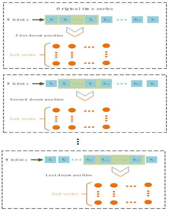
Figure 7.
Schematic diagram of the decomposition mechanism based on the sliding window.
In the LSTM prediction model, the learning rate, the number of hidden layers, and the number of training iterations are key hyperparameters affecting model performance.
The learning rate controls the parameter update step size when the gradient decreases. If it is too large, it is easy to skip the optimal solution and cause gradient explosion; if it is too small, the convergence is slow and it is difficult to capture long-term dependence.
The maximum number of hidden layers determines the depth and complexity of the network. With excessive parameter space, the dimension increases, it is easy to overfit, and the gradient disappears; with too little, it is difficult to capture complex nonlinear relationships, and the performance of training and testing is poor. The number of training iterations leads to the model not fully learning the effective patterns in the data, and the prediction performance is reduced. If the number of training iterations is too large, the verification loss begins to rise. The model is overly sensitive to noise or outliers in the training data, and the generalization ability is reduced.
In order to verify the influence of the above four parameters on LSTM, taking the spring and autumn data as an example, four groups of statistical significance analysis of different parameters were performed for each parameter. The same set of parameters ran 10 times, and the results are shown in Figure 8.
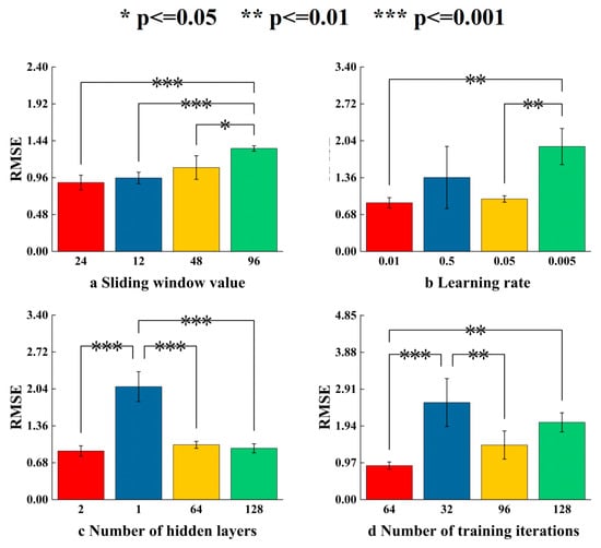
Figure 8.
Parameter analysis diagram affecting the performance of the model.
The influence of different sliding window values on the performance of the LSTM model can be seen in Figure 8a. It can be seen that there is a significant difference when the sliding window value is 96. When the value is 24, the performance is slightly better than that of 12 and 48. In order to predict the accuracy, 24 data points were selected from the original data as windows. This size balances data capture and computational efficiency, and improves prediction performance.
It can be seen from Figure 8b that the learning rate and model performance do not show a linear relationship. It can be seen that when the learning rate decreases from 0.5 to 0.05, the RMSE index decreases. When the learning rate decreases to 0.005, the RMSE index suddenly rises higher than the learning rate of 0.5. It can be seen from Figure 8c that the performance of the model does not have a significant performance improvement due to the increase in the number of hidden layers. When the number of hidden layers increases from 2 to 64 or 128, the performance of the model does not show a significant improvement. In Figure 8d, it can be found that the performance of the model decreases significantly when the number for iterative training is 32 and 128, and there is a significant difference when the number for iterative training is 64.
Based on the above analysis, it can be found that the learning rate and other parameters have an impact on the performance of the model. At the same time, it was found that the impact is nonlinear, and the performance of the model cannot be improved by increasing or decreasing it. In order to balance the learning efficiency and computational complexity, through experimental comparison, the performance of the parameter value model in Table 9 is more balanced. Further, IHOA was used to optimize the LSTM parameters for the data set of each season to achieve better optimization results.
The e-QPSO used 10 iterations and an initial population of 10 []; the value range of the total number of modal decomposition K is [5, 20], and the search range of the penalty coefficient α is [500, 3000]. Finally, the optimal VMD parameter combinations for the four datasets are [705, 15], [1652, 16], [2784, 18], and [1324, 20], respectively. In order to simplify the explanation, this paper only shows the iterative comparison image decomposition results of autumn historical data in Figure 9.

Figure 9.
e-QPSO-optimized VMD decomposition results (autumn data).
Taking the minimum value of sample entropy as the objective function and taking the autumn data as an example, the iterative comparison diagram of VMD optimized by e-QPSO and VMD optimized by WOA [] is shown in Figure 10.
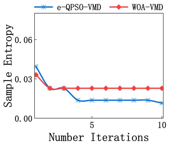
Figure 10.
Comparison of VMD optimized by e-QPSO and WOA (autumn data).
3.2. Evaluating Indicator
The root mean square error (RMSE), mean absolute percentage error (MAPE), and mean absolute error (MAE), were used to evaluate the effect of wind-speed forecast. RMSE, MAPE, and MAE were used as evaluation indicators. The smaller their values are, the better the prediction effect is.
In Equations (19)–(21), is the number of samples, the true value, and is the predicted value.
4. Results
In this section, in order to fully verify the validity of the model, a comparative experiment of six models was carried out. It should be emphasized that all the decomposition processes adopted the decomposition mechanism based on the sliding window proposed in this paper to avoid data leakage. Two classical and commonly used prediction models, BPNN and LSTM, were selected as the benchmarks for the basic comparison of Experiment 1. Two single models, HOA-LSTM and IHOA-LSTM, with two optimization models but without decomposition technology, were selected. A decomposed but unimproved optimization model e-QPSO-VMD-HOA-LSTM (represented by eV-HOA-LSTM for writing later) and a WOA-VMD-IHOA-LSTM (represented by WV-IHOA-LATM for writing later) using IHOA using WOA to optimize VMD were introduced. The model proposed in this paper is compared with the prediction performance of these six models. In order to fully verify the validity of the prediction, four seasonal comparative experiments were carried out. In Figure 11, the comparison of Proposed and e-QPSO-VMD-HOA-LSTM in four seasons is shown. It can be found that Proposed is more suitable for real data in four seasons, indicating the effectiveness of the model.
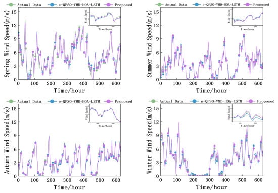
Figure 11.
Comparison of prediction results.
From the scatter plot of the real value and the predicted value of Figure 12, we can see the accuracy of Proposed. There is no deviation in the discrete points, and all points fit the straight line. It shows that the overall outcome can be more accurate prediction.
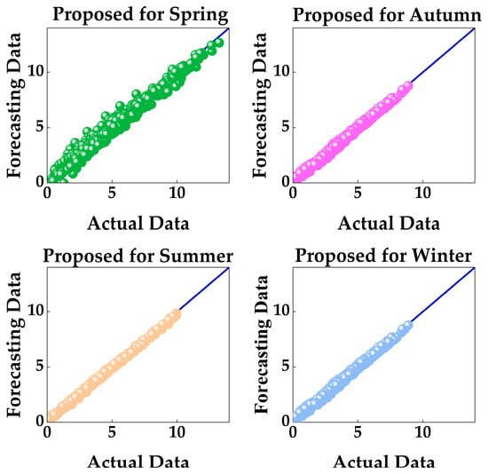
Figure 12.
Scatter plot of the true values and predicted values of the four seasons.
The proposed method was evaluated using 2023 wind speed data from Changchun, with prediction performance quantified through three metrics: root mean squared error (RMSE), mean absolute percentage error (MAPE), and mean absolute error (MAE). Figure 11 displays the prediction error distribution (box plot), while Figure 13 provides a comparative visualization of seven model performance indicators.
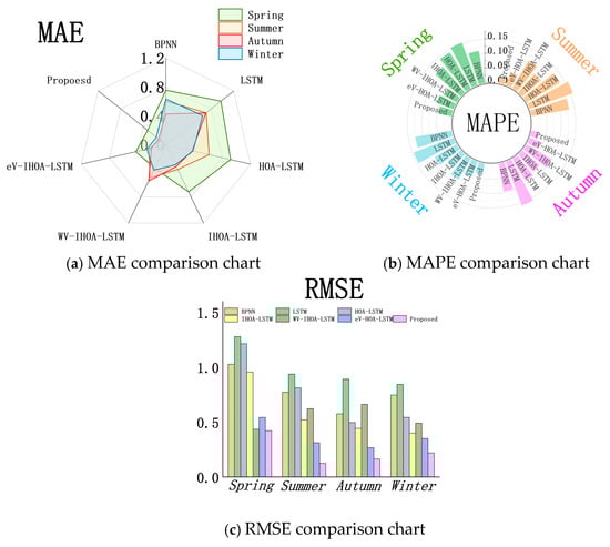
Figure 13.
Model index comparison chart.
As summarized in Table 10, the WV-IHOA-LATM model outperforms six benchmark time series forecasting methods across all metrics. In Figure 13, the RMSE (bar chart), MAPE (radial bar chart), and MAE (radar chart) results demonstrate the consistent superiority of the proposed model in all four seasons. This confirms that the e-QPSO algorithm enhances the decomposition capability of the IHOA-LSTM framework, enabling more accurate wind-speed predictions compared to the standalone IHOA-LSTM model under identical conditions.
Table 10.
Comparison table of indicators.
The performance of the model proposed in this paper has been significantly improved []. Taking RMSE as an example, compared with the four seasons of IHOA-LSTM, it has increased by 22.38%, 76.11%, 63.12%, and 45.17% respectively, indicating that the decomposition strategy adopted in this paper can improve the prediction accuracy more efficiently. By comparing the accuracy of eV-HOA-LSTM in four seasons, it can be seen thar its performance was improved by 22.38%, 60.16%, 38.56%, and 37.38%, respectively. The above shows that IHOA is better than HOA in optimizing the LSTM model. The wind-speed prediction performance was significantly improved.
Due to the inherent noise in the original wind speed input, the performance of a single comparison model is affected. The e-QPSO-VMD-HOA-LSTM model combined with VMD decomposition technology showed a stronger prediction ability, and its RMSE (0.5437) was further reduced by 46.8% compared with the undecomposed IHOA-LSTM (0.9556). Proposed achieved an RMSE of 0.4191 in the spring prediction, which was 22.9% lower than e-QPSO-VMD-HOA-LSTM. The VMD module exhibited strong noise resistance, high decomposition efficiency, and stability when processing raw wind-speed data, which inherently contains significant noise and nonlinear/non-stationary characteristics. By integrating the e-QPSO algorithm, the proposed e-QPSO-VMD method optimizes and improves performance. The hybrid model maintains superior performance across all seasons.
The box plot in Figure 14 compares the error data distribution. Each graph shows the distribution range of different target values, including the median, quartile, and overall fluctuation, which provides an intuitive basis for comparing the performance differences of the models. The boxplot in Figure 10 shows that the models proposed in this paper are more concentrated in the distribution of predicted wind-speed errors. Taking autumn as an example, the quartile range of the error boxplot is −1 to 1, which is significantly lower than the four models without decomposition (BPNN, LSTM, HOA-LSTM, IHOA-LSTM). It is also slightly better than the two models using optimized VMD (WV-IHOA-LSTM, eV-HOA-LSTM). In the four seasons, the model proposed in this paper is better than the other six models in terms of error performance. It is worth noting that in the wind-speed prediction in spring, WV-IHOA-LSTM is slightly better than the model proposed in this paper. Its quartile range is between 0.1 and 0.4, while the model in this paper is between −0.3 and 0.2.

Figure 14.
Box line diagram.
In the four seasons, the effect of all models in spring (January–March) is not as good as that in the other three months. The reason may be that the wind speed in spring fluctuates greatly. It can be seen from the comparison of spring wind speed in Figure 10 that, compared with the other three seasons, wind speed changes more in a short time, and the peak value of wind speed is higher, which brings difficulties to the learning of the model. Compared with the wind-speed fluctuation in summer and autumn, the prediction effect of the model is better. The wind speed in winter has a low wind speed for some time. These too-low wind speeds also bring some troubles to the model prediction, resulting in a prediction result that is not as good as that in summer and autumn.
5. Conclusions
The energy crisis and environmental pollution caused by fossil fuels can be alleviated through the development and utilization of wind energy. However, wind turbines and wind-power grid integration are significantly influenced by wind speed. The accuracy of wind-speed prediction is crucial for the stable operation of wind turbines. This paper proposes a hybrid model, e-QPSO-VMD-IHOA-LSTM. The superiority of this model is verified by the wind-speed data of Changchun City in the four seasons of 2023. Additionally, this paper conducts a comparative analysis of six other models and three evaluation indicators. The following conclusions can be drawn:
(1): By comparing the first 12 standard functions of CEC2005, three strategies are used to improve IHOA, among which five algorithms including HOA have a better optimization ability. Compared with the five algorithms, the optimization results of the single-peak function (F1–F4) are lower than the order of 10, which is better than HOA, and the optimization results of the multi-peak function (such as F9–F11) are 0, which is also better than HOA and the other five algorithms. It shows better performance in the optimization of test functions. The model proposed in this paper is more adaptable to the nonlinear characteristics of wind speed than other basic models. The comparison of different optimization algorithms shows that both HOA and IHAO can be used to optimize the parameters of LSTM and improve the accuracy of wind-speed prediction. By comparing the parameter indicators in Figure 10 and Table 10 it can be concluded that IHOA can optimize the parameters of the prediction model more effectively than HOA;
(2): Meanwhile, the e-QPSO algorithm was employed to optimize VMD, demonstrating better adaptability compared to the WOA algorithm. The e-QPSO-VMD method can effectively enhance the model’s wind-speed prediction performance. In the four datasets, the RMSE, MAPE, and MAE of e-QPSO-VMD-IHOA-LSTM are significantly lower than those of WOA-VMD-IHOA-LSTM. By comparing the indicators of this model with those of the WOA-VMD-HOA-LSTM model, it can be concluded that e-QPSO-VMD-IHOA-LSTM exhibits superior performance. Among them, RMSE decreased by 53.49% on average, MAP decreased by 53.68% on average, and MAE decreased by 55.64% on average. This result confirms that e-QPSO-VMD-IHOA-LSTM has better performance in wind speed prediction.
Shortcomings of this study:
(1): This study does not adjust the model for wind-speed fluctuations caused by seasonal factors. The seasonal differences in wind speed caused by external factors such as monsoons or other environmental factors should be considered to improve the prediction ability of the model;
(2): In this study, the structure of the LSTM model has not been adjusted to better adapt to wind-speed prediction. The study only considers the use of LSTM, and the learning of wind speed by model structure should be considered to adjust the structure to achieve better prediction results;
(3): It fails to simplify the calculation structure, resulting in high computational complexity and an increased time cost. The processor used in this study was the AMD Ryzen 7 78408 core processor, 3.8 GHz. The Matlab2023 b platform was used. The calculation formula of the model proposed in this paper is Equation (22).
where E is the number of training iterations, T is the length of the sequence, H is the number of hidden units, and D is the input feature dimension. Consider the case where all values are maximum. The time complexity of this model is about 1.32 × 10¹². The single run time of the model is long. It is not conducive to data collection and analysis.
The follow-up research direction is as follows. In the future, we will continue to study the topic of wind-speed prediction, focusing on wind-speed prediction in a short period of time.
Author Contributions
Conceptualization, G.L. and Y.C.; methodology, G.L. and Y.C.; software, G.L.; validation, Y.C. and X.D.; formal analysis, G.L. and X.D.; investigation, Y.C. and C.W.; resources, Y.C.; data curation, X.D.; writing—original draft preparation, G.L.; writing—review and editing, Y.Z. (Yao Zhang) and J.W.; visualization, Y.Z. (Yang Zhao); supervision, Y.C. and Y.S.; project administration, Y.C.; funding acquisition, Y.C. All authors have read and agreed to the published version of the manuscript.
Funding
This paper was supported by the Key Research and Development Project of Science and Technology Development in Jilin Province (Project Number: 20240304183SF). This paper was also supported by the Research on Key Technologies for Efficient Utilization of Wastewater Heat Sources (Project Number: 2024YFC3810202-05).
Institutional Review Board Statement
Not applicable.
Informed Consent Statement
Not applicable.
Data Availability Statement
Data is contained within the article.
Conflicts of Interest
The authors declare no conflicts of interest.
References
- Ping, Y. A Review of Wind Speed and Wind Power Forecasting Methods for Wind Farms. Electron. Technol. Softw. Eng. 2019, 214, 117766. [Google Scholar]
- Veers, P.; Dykes, K.; Lantz, E.; Barth, S.; Bottasso, C.L.; Carlson, O.; Clifton, A.; Green, J.; Green, P.; Holttinen, H.; et al. Grand Challenges in the Science of Wind Energy. Science 2019, 366, eaau2027. [Google Scholar] [CrossRef] [PubMed]
- de Falani, S.Y.A.; González, M.O.A.; Barreto, F.M.; de Toledo, J.C.; Torkomian, A.L.V. Trends in the Technological Development of Wind Energy Generation. Int. J. Technol. Manag. Sustain. Dev. 2020, 19, 43–68. [Google Scholar] [CrossRef]
- Wang, Y.; Wang, J.; Li, Z. A Novel Hybrid Air Quality Early-Warning System Based on Phase-Space Reconstruction and Multi-Objective Optimization: A Case Study in China. J. Clean. Prod. 2020, 260, 121027. [Google Scholar] [CrossRef]
- Jiang, P.; Liu, Z.; Wang, J.; Zhang, L. Decomposition-Selection-Ensemble Forecasting System for Energy Futures Price Forecasting Based on Multi-Objective Version of Chaos Game Optimization Algorithm. Resour. Policy 2021, 73, 102234. [Google Scholar] [CrossRef]
- Huang, S.-C.; Chiou, C.-C.; Chiang, J.-T.; Wu, C.-F. A Novel Intelligent Option Price Forecasting and Trading System by Multiple Kernel Adaptive Filters. J. Comput. Appl. Math. 2020, 369, 112560. [Google Scholar] [CrossRef]
- Wu, B.; Wang, L.; Zeng, Y.-R. Interpretable Wind Speed Prediction with Multivariate Time Series and Temporal Fusion Transformers. Energy 2022, 252, 123990. [Google Scholar] [CrossRef]
- Jiang, Z.; Che, J.; Wang, L. Ultra-Short-Term Wind Speed Forecasting Based on EMDVAR Model and Spatial Correlation. Energy Convers. Manag. 2021, 250, 114919. [Google Scholar] [CrossRef]
- Wang, J.; Yang, Z. Ultra-Short-Term Wind Speed Forecasting Using an Optimized Artificial Intelligence Algorithm. Renew. Energy 2021, 171, 1418–1435. [Google Scholar] [CrossRef]
- Liu, Z.; Jiang, P.; Zhang, L.; Niu, X. A Combined Forecasting Model for Time Series: Application to Short-Term Wind Speed Forecasting. Appl. Energy 2020, 259, 114137. [Google Scholar] [CrossRef]
- Jiang, P.; Liu, Z.; Niu, X.; Zhang, L. A Combined Forecasting System Based on Statistical Method, Artificial Neural Networks, and Deep Learning Methods for Short-Term Wind Speed Forecasting. Energy 2021, 217, 119361. [Google Scholar] [CrossRef]
- Sobolewski, R.A.; Tchakorom, M.; Couturier, R. Gradient Boosting-Based Approach for Short- and Medium-Term Wind Turbine Output Power Prediction. Renew. Energy 2023, 203, 142–160. [Google Scholar] [CrossRef]
- Wang, J.; Qin, S.; Zhou, Q.; Jiang, H. Medium-Term Wind Speeds Forecasting Utilizing Hybrid Models for Three Different Sites in Xinjiang, China. Renew. Energy 2015, 76, 91–101. [Google Scholar] [CrossRef]
- Azad, H.B.; Mekhilef, S.; Ganapathy, V.G. Long-Term Wind Speed Forecasting and General Pattern Recognition Using Neural Networks. IEEE Trans. Sustain. Energy 2014, 5, 546–553. [Google Scholar] [CrossRef]
- Yan, J.; Ouyang, T. Advanced Wind Power Prediction Based on Data-Driven Error Correction. Energy Convers. Manag. 2019, 180, 302–311. [Google Scholar] [CrossRef]
- Zhao, W.; Wei, Y.-M.; Su, Z. One Day Ahead Wind Speed Forecasting: A Resampling-Based Approach. Appl. Energy 2016, 178, 886–901. [Google Scholar] [CrossRef]
- Demolli, H.; Dokuz, A.S.; Ecemis, A.; Gokcek, M. Wind Power Forecasting Based on Daily Wind Speed Data Using Machine Learning Algorithms. Energy Convers. Manag. 2019, 198, 111823. [Google Scholar] [CrossRef]
- Su, J.; Zheng, S.; Yan, G.; Xiong, G.; Cai, T. Research on Day-Ahead Forecast of Wind Power Based on FCM-Equivalent Wind Speed Mode. Adv. Power Syst. Hydraul. Eng. 2022, 38, 110–120. [Google Scholar]
- Cassola, F.; Burlando, M. Wind speed and wind energy forecast through Kalman filtering of numerical weather prediction model output. Appl. Energy 2012, 99, 154–166. [Google Scholar] [CrossRef]
- Zhao, J.; Guo, Y.; Xiao, X.; Wang, J.; Chi, D.; Guo, Z. Multi-step wind speed and power forecasts based on a WRF simulation and an optimized association method. Appl. Energy 2017, 197, 183–202. [Google Scholar] [CrossRef]
- Jain, L.C.; Medsker, L.R. Recurrent Neural Networks: Design and Applications. In Recurrent Neural Networks: Design and Applications; CRC Press: Boca Raton, FL, USA, 1999. [Google Scholar]
- Graves, A. Supervised Sequence Labelling with Recurrent Neural Networks. In Studies in Computational Intelligence; Springer: Berlin/Heidelberg, Germany, 2012. [Google Scholar]
- Pan, Z.; Yu, W.; Yi, X.; Khan, A.; Yuan, F.; Zheng, Y. Recent Progress on Generative Adversarial Networks (GANs): A Survey. IEEE Access 2019, 7, 36322–36333. [Google Scholar] [CrossRef]
- Li, G.; Shi, J. Compare Three Artificial Neural Networks for Wind Speed Forecasting. Appl. Energy 2010, 87, 2313–2320. [Google Scholar] [CrossRef]
- Liu, H.; Mi, X.; Li, Y. Wind Speed Forecasting Method Based on Deep Learning Strategy Using Empirical Wavelet Transform, Long Short-Term Memory Neural Network, and Elman Neural Network. Energy Convers. Manag. 2018, 156, 498–514. [Google Scholar] [CrossRef]
- Liu, H.; Tian, H.; Li, Y. An EMD-Recursive ARIMA Method to Predict Wind Speed for Railway Strong Wind Warning System. J. Wind Eng. Ind. Aerod. 2015, 141, 27–38. [Google Scholar] [CrossRef]
- Li, J.; Wang, J.; Zhang, H.; Li, Z. An Innovative Combined Model Based on Multi-Objective Optimization Approach for Forecasting Short-Term Wind Speed: A Case Study in China. Renew. Energy 2022, 201, 766–779. [Google Scholar] [CrossRef]
- Hu, H.; Wang, L.; Tao, R. Wind Speed Forecasting Based on Variational Mode Decomposition and Improved Echo State Network. Renew. Energy 2021, 164, 729–751. [Google Scholar] [CrossRef]
- Du, L.K. Research and Application of Sea—Level Wind Speed Prediction Based on ES—XGBoost. Master’s Thesis, Nanchang University, Nanchang, China, 2023. [Google Scholar]
- Yanovsky, I.; Dragomiretskiy, K. Variational Destriping in Remote Sensing Imagery: Total Variation with L1 Fidelity. Remote Sens. 2018, 10, 300. [Google Scholar] [CrossRef]
- Agrawal, R.K.; Kaur, B.; Agarwal, P. Quantum Inspired Particle Swarm Optimization with Guided Exploration for Function Optimization. Appl. Soft Comput. 2021, 102, 107122. [Google Scholar] [CrossRef]
- Oladejo, S.O.; Ekwe, S.O.; Mirjalili, S. The Hiking Optimization Algorithm: A Novel Human-Based Metaheuristic Approach. Knowl.-Based Syst. 2024, 296, 111880. [Google Scholar] [CrossRef]
- Liu, W.; Guo, Z.; Jiang, F.; Liu, G.; Jin, B.; Wang, D. Grey Wolf Algorithm Improved by Collaborative Encirclement Strategy and Its PID Parameter Optimization. J. Comput. Sci. Explor. 2023, 17, 620–634. [Google Scholar]
- Sun, J.; Feng, B.; Xu, W. Particle Swarm Optimization with Particles Having Quantum Behavior. In Proceedings of the 2004 Congress on Evolutionary Computation, Portland, OR, USA, 19–23 June 2004; IEEE: Portland, OR, USA, 2004; Volume 1, pp. 325–331. [Google Scholar]
- Yang, D.; Li, M.; Guo, J.; Du, P. An Attention-Based Multi-Input LSTM with Sliding Window-Based Two-Stage Decomposition for Wind Speed Forecasting. Appl. Energy 2024, 375, 124057. [Google Scholar] [CrossRef]
- Zhang, Y.; Han, P.; Wang, D.; Wang, S. Short-Term Wind Speed Prediction in Wind Farms Based on Variational Mode Decomposition and LSSVM. Acta Energiae Solaris Sin. 2018, 39, 194–202. [Google Scholar]
- Nie, X.; Hong, Y. Long-Term Electric Load Forecasting Based on WOA-VMD-GBDT. Technol. Wind 2024, 4, 1–10. [Google Scholar]
- Zhang, Y.M.; Wang, H. Multi-Head Attention-Based Probabilistic CNN-BiLSTM for Day-Ahead Wind Speed Forecasting. Energy 2023, 278, 127865. [Google Scholar] [CrossRef]
Disclaimer/Publisher’s Note: The statements, opinions and data contained in all publications are solely those of the individual author(s) and contributor(s) and not of MDPI and/or the editor(s). MDPI and/or the editor(s) disclaim responsibility for any injury to people or property resulting from any ideas, methods, instructions or products referred to in the content. |
© 2025 by the authors. Licensee MDPI, Basel, Switzerland. This article is an open access article distributed under the terms and conditions of the Creative Commons Attribution (CC BY) license (https://creativecommons.org/licenses/by/4.0/).