Abstract
This paper introduces a novel end-to-end fault diagnosis framework that integrates Bidirectional Long Short-Term Memory (BiLSTM) networks with Time-Domain Reflectometry (TDR) for the detection, characterization, and localization of wiring faults. The method is designed to operate directly on TDR signals, requiring no manual feature extraction or preprocessing. A forward model is used to simulate TDR responses across various fault scenarios and topologies, serving as the basis for supervised learning. The proposed BiLSTM-based model is trained and validated on common wiring network topologies, demonstrating high diagnostic performance. Experimental results show a diagnostic accuracy of 98.97% and a macro-average sensitivity exceeding 98%, outperforming conventional machine learning techniques. In addition to technical performance, the proposed approach supports sustainable and predictive maintenance strategies by reducing manual inspection efforts and enabling real-time automated diagnostics.
1. Introduction
Wiring networks serve as the invisible yet critical backbone of reliable electrical and communication functionalities in modern industrial systems, transportation infrastructures, and smart environments. From aerospace to automotive systems and from civil engineering installations to renewable energy grids, the integrity of complex wiring architectures directly impacts safety, performance, and operational continuity. As these systems grow in scale and complexity, the early detection, localization, and classification of faults within wiring networks, commonly referred to as wiring network diagnosis, has become a field of strategic importance.
Wiring network faults are generally classified into two main categories: soft faults and hard faults. Soft faults typically arise from localized degradation such as insulation wear, minor conductor damage, or gradual changes in impedance, and often remain undetected until they advance. If left unaddressed, these subtle anomalies can deteriorate and eventually evolve into hard faults, typically characterized by open or short circuits. These failures can compromise signal integrity, cause power interruptions, or trigger system-wide malfunctions. The risk is especially critical in domains where the reliability of electrical interconnections is essential, such as in aerospace systems, medical devices, or renewable energy infrastructures. As such, wiring defects represent more than just technical challenges; in high-stakes applications, they can lead to catastrophic consequences. This is vividly illustrated by several documented aircraft accidents (see [1]) in which undetected wiring faults contributed to system failures or onboard fires, underscoring the urgent need for robust diagnostic frameworks in safety-critical environments.
The implementation of advanced diagnostic and preventive strategies is not only crucial for ensuring operational safety but also forms a fundamental pillar of sustainable engineering. A robust diagnostic framework enables the early identification and precise localization of faults, allowing operators to intervene before degradation escalates into critical failures. This proactive approach significantly reduces unplanned downtime, minimizes service disruptions, and extends the operational lifespan of wiring components. In addition to reliability, diagnostic precision enhances network performance by targeting only the affected areas for repair or replacement, thereby optimizing resource allocation and minimizing unnecessary material usage. This targeted maintenance reduces labor costs and contributes to substantial savings in both time and operational expenses. From a sustainability perspective, such an approach directly supports environmental objectives; by maintaining optimal electrical continuity and minimizing resistive losses, it reduces energy waste and lowers the carbon footprint associated with over-maintenance, equipment disposal, and energy inefficiencies.
A variety of diagnostic methods have been developed to detect and locate faults in wiring networks, each offering distinct tradeoffs in terms of accuracy, complexity, and applicability. These include model-based approaches [2], signal processing techniques [3], statistical learning frameworks [4], and electromagnetic methods [5]. Among these, reflectometry has emerged as a particularly robust and versatile strategy due to its non-intrusive nature, ease of deployment, and high spatial resolution [1]. Reflectometry techniques operate by injecting a known excitation signal into the network and analyzing the reflected waveforms generated by impedance discontinuities. When the signal encounters irregularities such as faults, branches, or degraded sections, partial reflections occur that carry diagnostic information back to the source. This operating principle enables fault localization from a single access point, making reflectometry especially advantageous in scenarios where physical access to the entire wiring system is constrained [1].
Several variants of reflectometry exist, each defined by the type of test signal and the domain in which measurements are interpreted. These include Time-Domain Reflectometry (TDR) [6], Spectrum TDR [7], Multicarrier TDR [8], Frequency-Domain Reflectometry [9], Optical Sequence TDR [10], and Joint Time-Frequency Reflectometry [11]. It is worth noting that many reflectometry methods can be transformed into TDR-equivalent signals through signal processing techniques such as the Fourier transform. A comprehensive review of various reflectometry methods employed for wiring network diagnosis is presented in [5]. While each method has specific advantages depending on the application context, TDR is widely adopted due to its simplicity, speed, cost efficiency, and strong diagnostic performance. It provides fast and high-resolution detection while requiring only minimal instrumentation, making it suitable for both laboratory studies and embedded applications in industrial environments. TDR signals can be obtained either experimentally or by simulation following numerical approaches or analytical models [12,13,14,15,16], depending on constraints such as cost, access, and reproducibility.
Although TDR remains a widely adopted method for wiring network diagnosis, its standalone diagnostic capability is inherently limited, particularly in the presence of complex topologies or distributed impedance discontinuities. TDR responses are prone to ambiguities due to overlapping reflections from branches, terminations, or distributed defects, making accurate interpretation and fault isolation a non-trivial task. To address these limitations, hybrid approaches have been developed that integrate TDR with advanced computational techniques aimed at enhancing diagnostic accuracy. These methodologies can be broadly classified into two families: inverse problem-based iterative algorithms and data-driven machine learning frameworks. Iterative approaches leverage a parametric forward model of the wiring network to synthetically generate expected TDR responses. Optimization algorithms such as Genetic Algorithms (GAs) [17] and Particle Swarm Optimization (PSO) [18] are then employed to minimize the misfit between simulated and measured responses. While they offer high localization accuracy, such methods are often computationally expensive, sensitive to initial conditions, and dependent on careful tuning of hyperparameters. Moreover, their iterative nature renders them unsuitable for real-time or embedded implementations, especially in safety-critical or time-constrained environments. In parallel, machine learning-based techniques have gained significant traction for their ability to model the inverse problem without explicitly solving it. Neural networks [19], Support Vector Machines (SVM) [20,21,22], random forests [23], k-Nearest Neighbor (k-NN) models [24], and one-dimensional convolutional neural networks [25] are commonly used to learn the nonlinear mappings between TDR responses and fault characteristics. These models are typically trained offline on synthetically generated or experimentally acquired datasets, and offer rapid inference once deployed. They are particularly suited for high-dimensional feature spaces and complex wiring configurations. However, their effectiveness depends heavily on the representativeness and diversity of the training set, and challenges remain in terms of model interpretability and generalization across varying network topologies. Additionally, feature extraction and selection often rely on domain expertise, which may limit automation and scalability.
This paper proposes a novel diagnostic framework that combines TDR with BiLSTM networks for fault detection, characterization, and localization in complex wiring networks. This integration addresses key challenges in interpreting TDR responses. The proposed approach leverages the sequence modeling capabilities of BiLSTM to extract temporal dependencies and bidirectional correlations inherent in reflected waveforms, enabling a more robust and precise fault classification process. The proposed methodology is structured into three stages. First, a comprehensive dataset is generated using a forward model that simulates TDR responses under various fault conditions and network configurations. In the second stage, this dataset is used to train a BiLSTM model which captures long-term dependencies in both past and future signal contexts. This bidirectional architecture enhances the model’s ability to recognize complex reflection patterns that may arise from multiple fault types or branching topologies. Finally, the trained BiLSTM network is applied to unseen TDR responses for real-time fault diagnosis. The main contributions and advantages of this approach are as follows:
- Temporal Modeling: Unlike traditional machine learning models, BiLSTM processes the TDR response as a temporal sequence, capturing both forward and backward dependencies. This allows it to interpret subtle, delayed, or overlapping reflections that are otherwise difficult to detect.
- High Accuracy and Generalization: BiLSTM achieves high accuracy across a variety of fault types and wiring configurations thanks to its memory gates and recurrent structure.
- Real-Time Capability and Reduced Need for Feature Engineering: The BiLSTM model automatically learns relevant features from raw TDR signals, eliminating the need for hand-crafted features or extensive preprocessing. After training, the BiLSTM model provides fast inference, making it suitable for onboard and real-time diagnostics.
- Scalability and Robustness: The proposed approach can be extended to complex or large-scale wiring networks and maintains stable performance across varying fault positions, severity levels, and network topologies.
The remainder of this paper is organized as follows: Section 2 introduces the forward modeling approach used to simulate wiring network behavior; Section 3 presents a comprehensive overview of the employed BiLSTM neural network architecture; the methodological framework is detailed in Section 4, followed by a discussion of the experimental results in Section 5; finally, Section 6 concludes the paper and outlines potential directions for future research.
2. Generation of TDR Responses via Forward Modeling
To generate the reflectometry response of a wiring network, several modeling approaches have been proposed in the literature. In this study, we adopt a method based on an equivalent electrical representation using RLGC parameters. The resulting model is governed by the following system of wave propagation equations:
where and are vectors representing the voltages and currents along the network lines, respectively. These equations are numerically solved using the Finite-Difference Time Domain (FDTD) method. Compared to analytical formulations, the FDTD approach offers greater flexibility, allowing signal behavior to be evaluated at any point along the network and enabling the modeling of a wide range of fault scenarios, including those involving complex topologies and distributed impedance discontinuities. To validate the accuracy of the forward model, a comparison is performed between the simulated TDR response of a wiring network and its experimentally measured counterpart. The impulse response is obtained by measuring the S11 parameter in the frequency domain from 300 kHz to 500 MHz using a Vector Network Analyzer (VNA). The results of this comparison are shown in Figure 1, where both signals are presented for direct visual inspection. The close agreement between the simulated and measured waveforms demonstrates the model’s ability to reliably replicate real-world reflectometry responses, confirming its suitability for use in diagnostic analysis.
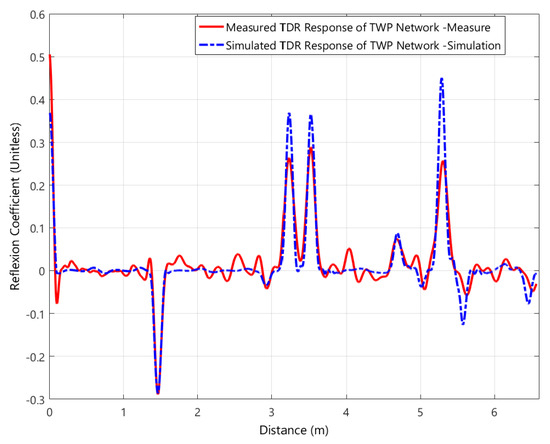
Figure 1.
Comparison of simulation results and measurements for the TDR responses.
It is worth noting that the validation of the forward model has been comprehensively addressed and confirmed in [26], providing strong evidence of its reliability and accuracy.
3. Bidirectional Long Short-Term Memory (BiLSTM)
BiLSTM networks are an advanced extension of standard LSTM architectures designed to process sequential data in both the forward and backward directions. As shown in Figure 2, this dual processing enables BiLSTMs to exploit both past and future contextual information within a sequence, enhancing their ability to model long-range dependencies and temporal correlations. This bidirectional structure offers a significant advantage over traditional LSTMs, which are limited to unidirectional contexts.
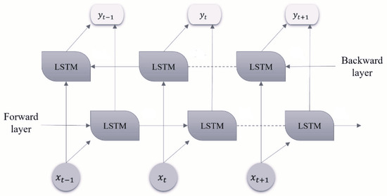
Figure 2.
Basic structure of the BiLSTM network.
Thanks to their ability to capture both past and future contexts, BiLSTM networks have proven to be highly effective in a range of time-dependent tasks. In natural language processing [27], they improve syntactic and semantic understanding by considering the full context of the sentence. They are also widely used in speech recognition [28] and time series forecasting [29] thanks to their ability to model complex temporal dependencies. In the field of fault diagnosis, BiLSTMs have demonstrated strong performance across a wide range of domains, including rotating machinery monitoring [30], chemical process supervision [31], wind turbine fault detection [32], photovoltaic array monitoring [33], bearing failure analysis [34], and even biomedical applications such as cardiac arrhythmia classification [35]. Their capacity to learn from full-sequence dependencies improves detection accuracy, reduces false positives, and improves the robustness of diagnostic systems, making them a powerful tool for real-time data-driven monitoring of dynamic and safety-critical infrastructures.
4. Methodology
The proposed methodology consists of two distinct processes: an offline modeling process and an online monitoring process, as depicted in Figure 3.
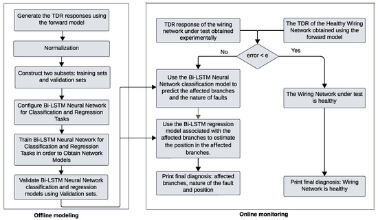
Figure 3.
Overview of the workflow of the proposed methodology.
4.1. Offline Modeling
The objective of the offline modeling process is to design, develop, and validate several BiLSTM neural network models for both classification and regression tasks. More precisely, the forward model is employed to simulate the TDR responses required for training the BiLSTM-based classifiers and regressors. This dataset includes representative examples that link reflectometry signals to fault types, fault locations, and the lengths of affected branches. The dataset is divided into two subsets: one for training and the other for validation. The training process involves the initial development of BiLSTM-based classification and regression models. These models are then evaluated using the validation subset to assess their accuracy and generalization capabilities. During the offline modeling phase, depending on the complexity of the wiring network configuration, it is crucial to prepare at least one BiLSTM classification model and at least one BiLSTM regression model for each affected branch:
- The BiLSTM-based classification model is designed to identify the affected branches and predict the type of faults. The training dataset used for this model consists of examples that associate TDR signals with the corresponding faulty branches and their respective fault types.
- BiLSTM-based regression models are developed to estimate the lengths of the affected branches. The training dataset for these models consists of examples that relate TDR responses to the corresponding branch lengths.
The configuration of the BiLSTM neural network models and their associated parameter settings are derived from comprehensive experimental evaluations. The trained models are assessed using a separate validation dataset to evaluate their performance in the classification task. As depicted in Figure 4a, the proposed architecture of the BiLSTM neural network for classification tasks employs multiple layers to enhance learning and generalization. The architecture commences with two BiLSTM layers. The first BiLSTM layer captures short-term temporal dependencies in both forward and backward directions, providing a thorough understanding of the temporal dynamics of the signal. The second BiLSTM layer builds upon this by capturing more complex and long-term dependencies, which refines the learned features. To address overfitting, dropout layers are incorporated after each BiLSTM layer with a dropout rate of 0.5. The dropout layers randomly deactivate neurons during training, thereby promoting generalization. Following the BiLSTM layers, two fully connected (dense) layers are employed. The initial fully connected layer transforms the features extracted by the BiLSTM layers into a higher-dimensional space, facilitating the learning of intricate patterns. This layer is succeeded by a ReLU (Rectified Linear Unit) activation layer which introduces nonlinearity, enabling the network to model complex relationships within the TDR responses. The subsequent fully connected layer further refines these features, preparing them for the final classification. The softmax layer is subsequently applied to convert the output scores into probabilities, allowing for a probabilistic interpretation of the classification results. Finally, the classification layer computes the loss and evaluates the model’s performance, ensuring that the network is optimized for the accurate classification of TDR responses. This combination of layers ensures a robust and effective model capable of addressing the complexities inherent in TDR responses. A BiLSTM neural network with a similar architecture is adopted for the regression task, as shown in Figure 4b. In contrast to the classification architecture, the softmax layer is removed and the classification layer is replaced with a regression layer to produce continuous-valued outputs that are suitable for regression.
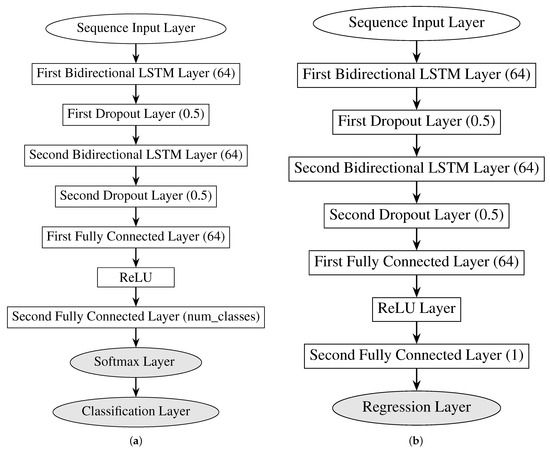
Figure 4.
BiLSTM neural network architecture for fault diagnosis in wiring networks, addressing classification and regression tasks: (a) BiLSTM neural network architecture for the diagnosis of wiring network faults, relevant to the classification task; (b) BiLSTM neural network architecture for the diagnosis of wiring network faults, relevant to the regression task.
4.2. Online Monitoring
The online monitoring process for diagnosing faults in wiring networks typically consists of three main phases: detection, localization, and characterization. In this study, a novel approach is proposed to address these stages, as illustrated in Figure 3 and detailed below.
Detection Phase: In this phase, the experimentally obtained TDR response of the wiring network under examination is compared with that of a fault-free reference network derived using the forward model. This comparison utilizes the Root Mean Square Error (RMSE) calculated between the two responses. Should the RMSE fall below a predetermined threshold, the network is considered to be in a healthy state. Conversely, an RMSE exceeding this threshold signifies the presence of a fault, necessitating progression to the localization and characterization phases.
Localization and Characterization Phases: The design parameters involved in the localization and characterization phases depend on the nature of the fault affecting the wiring network. For soft faults such as local impedance variations, the key parameters include the precise fault location and its associated impedance. In contrast, for hard faults such as open or short circuits, the relevant parameters consist of the lengths of the affected branches (used for localization) and the characteristics of the connected loads (used for fault characterization). This study specifically addresses the diagnosis of hard faults; accordingly, the localization and characterization process is structured into two main steps: (1) identifying the affected branches and determining the fault types, and (2) estimating the exact location of the fault within each affected branch. To achieve this, we employ the BiLSTM-based classification and regression models previously developed during the offline processes. The TDR response is fed into the BiLSTM classifier to predict the affected branches and their corresponding fault types, then the associated BiLSTM regression model is used to estimate the precise fault location within each identified branch.
5. Numerical Results
5.1. Diagnosis of a Y-Shaped Network Affected by One or Two Hard Faults
This analysis considers a Y-shaped wiring configuration consisting of three wires, each measuring 1.5 m in length: L1 = 1.5 m, L2 = 1.5 m, and L3 = 1.5 m. The L2 and L3 branches are connected to open circuits, as depicted in Figure 5.
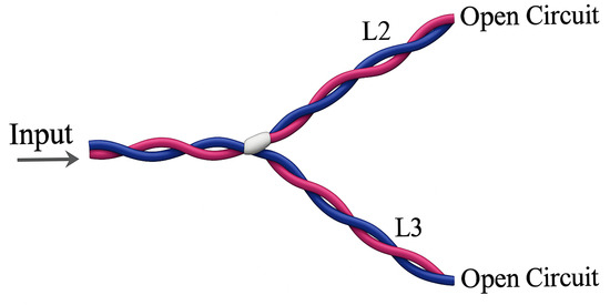
Figure 5.
Y-shaped wiring network.
5.1.1. Offline Modeling
To create a dataset for the Y-shaped network with one or two hard faults, the forward model simulates the behavior of the wiring network across various fault conditions, generating TDR responses. Each of these responses is then assigned a corresponding class label, resulting in a total of ten distinct labeled classes.
- Class 11: Represents an open-circuit type hard failure in L1. This class contains 144 labeled TDR signals.
- Class 12: Represents a short circuit-type hard failure in L1. This class contains 144 labeled TDR signals.
- Class 21: Represents an open circuit-type hard failure in L2. This class contains 212 labeled TDR signals.
- Class 22: Represents a short circuit-type hard failure in L2. This class contains 212 labeled TDR signals.
- Class 31: Represents a hard fault of open circuit type in L3. This class contains 202 labeled TDR signals.
- Class 32: Represents a short circuit-type hard failure in L3. This class contains 202 labeled TDR signals.
- Class 231: Represents the presence of two hard faults of open circuit type, one in L2 and one in L3. This class contains 195 labeled TDR signals.
- Class 232: Represents the presence of two hard faults of the short circuit type, one in L2 and one in L3. This class contains 195 labeled TDR signals.
- Class 233: Represents the presence of two hard faults, with one open circuit fault in L2 and one short-circuit fault in L3. This class contains 174 labeled TDR signals.
- Class 234: Represents the presence of two hard faults, with one short circuit fault in L2 and one open circuit fault in L3. This class contains 174 labeled TDR signals.
Remark 1.
It should be noted that the class corresponding to a fault in L1 and in the secondary branches L2 or L3 cannot be taken into account, as the test signal cannot propagate to L2 and L3 if the main branch L1 is under a hard fault.
The dataset has been organized to facilitate the training and evaluation of the proposed BiLSTM models for both classification and regression tasks. It is divided into two subsets, with 80% of the data allocated for training and the remaining 20% used for validation. This split is a commonly adopted ratio in machine learning to ensure that a sufficient amount of data is used to train the model while reserving a representative portion for unbiased evaluation. The BiLSTM models are implemented with particular configurations, as detailed in Table 1. Notably, hyperparameter tuning is conducted through a grid search optimization process to determine the best parameter values for the training settings with the aim of maximizing accuracy and minimizing loss.

Table 1.
Training options for BiLSTM neural network classification model.
Figure 6 shows the results of the training process for the classification task using the proposed BiLSTM model. The upper sub-plot displays the accuracy for both the training and validation sets, while the lower subplot shows the corresponding loss values. A key observation is the clear alignment between the accuracy and loss metrics for both datasets, demonstrating the model’s strong performance and reliability across both the training and validation phases.
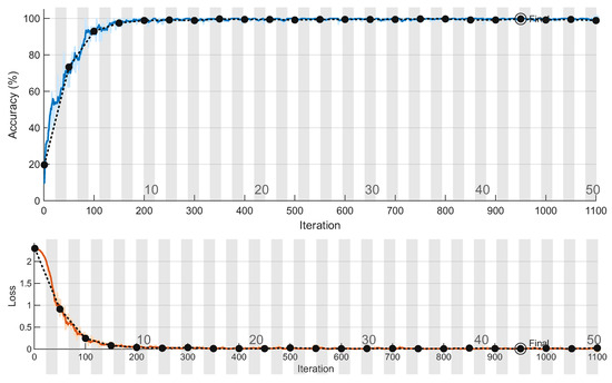
Figure 6.
Y-shaped wiring network, showing the training and validation accuracy and loss vs. the number of iterations.
Figure 7 displays the confusion matrix obtained from the validation phase of the proposed BiLSTM model. This matrix highlights the effectiveness of the BiLSTM model in correctly identifying the ten target classes. These results demonstrate the reliability and precision of the model in classifying the validation data, highlighting its strong overall performance.
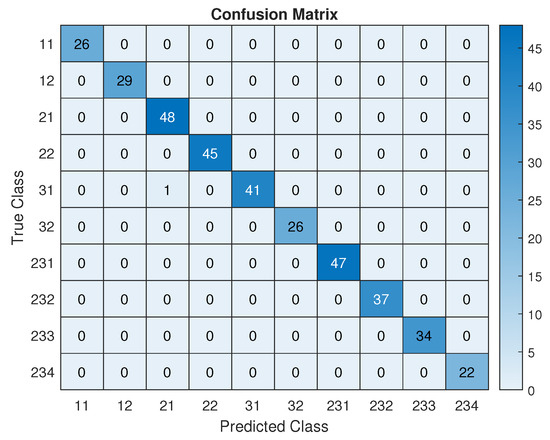
Figure 7.
Y-shaped wiring network showing the confusion matrix for the validation phase.
To evaluate the performance of classification, three key metrics are used: Precision, Sensitivity, and F1-score. To further assess the performance of the proposed model, we individually calculate these metrics for each class i, as follows:
- Precision measures the proportion of true positive predictions among all predicted positives.
- Sensitivity (also known as Recall) indicates the proportion of true positives among all actual positives.
- F1-score is the harmonic mean of precision and sensitivity.
In the above equations, refers to the number of TDR responses correctly identified as belonging to class i (true positives), refers to the number of TDR responses incorrectly classified as class i (false positives), and refers to the number of TDR responses from class i incorrectly classified as belonging to another class (false negatives). Calculating these metrics allows for a more detailed evaluation by highlighting the strengths and weaknesses of the model between different classes. As illustrated in Figure 8, the model consistently achieves high scores in all classes, indicating its ability to distinguish between fault types with a high degree of reliability and robustness.
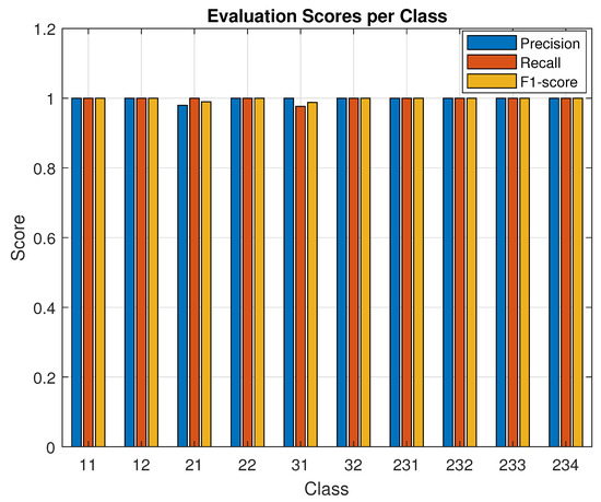
Figure 8.
Y-shaped wiring network, showing evaluation metrics (Precision, Sensitivity, F1-Score) for each class i.
Table 2 compares the accuracy of the proposed method against other methods during validation on a Y-shaped wiring network with a hard fault. The dataset is split into 80% for training and 20% for validation, with each classifier trained ten times using random splits. The results show the proposed method’s superior performance.

Table 2.
Comparative analysis of accuracy and sensitivity across different methods.
5.1.2. Online Monitoring
In the context of the Y-shaped wiring network, a hard fault is introduced on a specific branch. The experimental configuration depicted in Figure 9 utilizes an Agilent Technologies Vector Network Analyzer (E5071C) operating in the frequency domain over a range spanning from 100 kHz to 4.5 GHz.
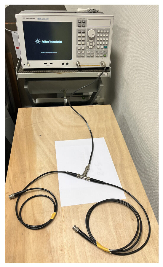
Figure 9.
Experimental setup for the Y-shaped wiring network.
Figure 10(top) depicts the experimental scenario involving two hard faults located on branches L2 and L3. To highlight the effects of these faults, Figure 10(bottom) presents a comparative analysis between the experimentally obtained TDR response of the faulty network and the fault-free response generated using the forward model.
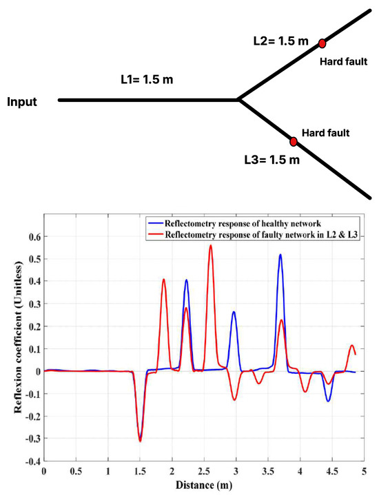
Figure 10.
(Top) Experimental scenario involving two hard faults on branches L2 and L3; (Bottom) TDR responses for healthy and faulty Y-shaped wiring networks.
To begin the diagnosis process, a comparison between the TDR response of the faulty network and the healthy wiring network is conducted using the RMSE metric. The RMSE value exceeds the established error threshold, indicating that faults are present in the network. Consequently, the algorithm proceeds to the localization and characterization phases. In order to determine the defective branches, the BiLSTM classifier model developed and validated during the offline modeling is applied. This classifier takes the experimental TDR response of the faulty network as input and outputs the class label corresponding to the affected branches. In this instance, the model outputs Class 231, indicating that L2 and L3 are the faulty branches and that the fault is of open circuit type. The next step is to estimate the new lengths of L2 and L3 using the BiLSTM regressor model. The regressor model pinpoints the fault locations at 1.1 meters for L2 and 0.73 meters for L3. The reconstructed wiring network is presented in Figure 11.
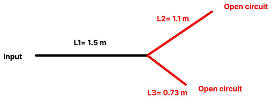
Figure 11.
The reconstructed wiring network.
5.2. Diagnosis of a YY-Shaped Network Affected by One or Two Hard Faults
The second scenario explores a YY-configuration wiring network encompassing five wires with lengths of L1 = 1.5 m, L2 = 1.5 m, L3 = 1.5 m, L4 = 0.75 m, and L5 = 1.5 m. As illustrated in Figure 12, branches L2, L3, L4, and L5 conclude with open circuits.
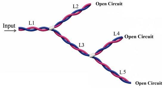
Figure 12.
YY-shaped wiring network.
5.2.1. Offline Modeling
To generate a dataset for the YY-shaped wiring network featuring either one or two hard faults, the forward model simulates the network’s behavior across various fault scenarios, resulting in corresponding TDR responses. Each TDR response is then assigned to a specific class label, leading to a total of twenty distinct labeled classes.
- Class 11: Represents an open circuit-type hard failure in L1. This class contains 144 labeled TDR signals.
- Class 12: Represents a short circuit-type hard failure in L1. This class contains 144 labeled TDR signals.
- Class 21: Represents an open circuit-type hard failure in L2. This class contains 212 labeled TDR signals.
- Class 22: Represents a short circuit-type hard failure in L2. This class contains 212 labeled TDR signals.
- Class 31: Represents a hard fault of open circuit type in L3. This class contains 202 labeled TDR signals.
- Class 32: Represents a short circuit-type hard failure in L3. This class contains 202 labeled TDR signals.
- Class 41: Represents a hard fault of open circuit type in L4. This class contains 140 labeled TDR signals.
- Class 42: Represents a short circuit-type hard failure in L4. This class contains 140 labeled TDR signals.
- Class 51: Represents a hard fault of open circuit type in L5. This class contains 72 labeled TDR signals.
- Class 52: Represents a short circuit-type hard failure in L5. This class contains 72 labeled TDR signals.
- Class 231: indicates the presence of two open circuit hard faults, with one fault on branch L2 and one fault on branch L3. This class contains 195 labeled TDR responses.
- Class 232: indicates the presence of two short circuit hard faults, with one fault on branch L2 and one fault on branch L3. This class contains 195 labeled TDR responses.
- Class 241: indicates the presence of two open circuit hard faults, with one fault on branch L2 and one fault on branch L4. This class contains 413 labeled TDR responses.
- Class 242: indicates the presence of two short circuit hard faults, with one fault on branch L2 and one fault on branch L4. This class contains 413 labeled TDR responses.
- Class 251: indicates the presence of two open circuit hard faults, with one fault on branch L2 and one fault on branch L5. This class contains 236 labeled TDR responses.
- Class 252: indicates the presence of two short circuit hard faults, with one fault on branch L2 and one fault on branch L5. This class contains 236 labeled TDR responses.
- Class 451: indicates the presence of two open circuit hard faults, with one fault on branch L4 and one fault on branch L5. This class contains 280 labeled TDR responses.
- Class 452: indicates the presence of two short circuit hard faults, with one fault on branch L4 and one fault on branch L5. This class contains 280 labeled TDR responses.
Remark 2.
It is important to note that scenarios involving two simultaneous faults, i.e., one on branch L1 and another on one of the secondary branches (L2, L3, L4, or L5), cannot be detected simultaneously under the assumptions of this work. Similarly, faults occurring at the same time on branches L3 and L4 or L5 are not jointly observable. This is because the scenario assumes hard faults, which cause full reflection of the test signal and consequently prevent it from propagating further along the network. For example, a hard fault on branch L1 blocks the signal from reaching any downstream branches; likewise, a hard fault on branch L3 stops the signal from reaching L4 and L5. Consequently, the diagnostic approach is to first locate and repair the fault closest to the source before conducting a new measurement to detect any additional faults further along the network.
Remark 3.
For the sake of clarity and to effectively demonstrate the diagnostic methodology applied to the YY-shaped network, it is assumed in the case of two hard faults that both faults are of the same type. Nevertheless, the proposed approach can be readily extended to accommodate scenarios involving two faults of different natures. For more complex topologies, we recommend adopting a divide-and-conquer strategy by decomposing the overall diagnostic task into several subproblems. Separate BiLSTM models based on TDR signals can be independently trained for each subnetwork to enable scalable and efficient fault detection and localization in large-scale and complex wiring networks.
The dataset is structured to support the training and evaluation of the BiLSTM model for both classification and regression tasks. It is divided into 80% for training and 20% for validation. Figure 13 illustrates the progression of the accuracy and loss metrics during these phases for the classification task. The strong consistency of these metrics between the training and validation sets underscores the robustness and reliability of the proposed BiLSTM model.
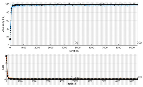
Figure 13.
YY-shaped wiring network, showing the training and validation accuracy and loss vs. the number of iterations.
Figure 14 displays the confusion matrix obtained from the validation phase of the proposed BiLSTM model. This matrix highlights the effectiveness of the BiLSTM model in correctly identifying the twenty target classes. These results demonstrate the reliability and precision of the model in classifying the validation data, highlighting its strong overall performance.
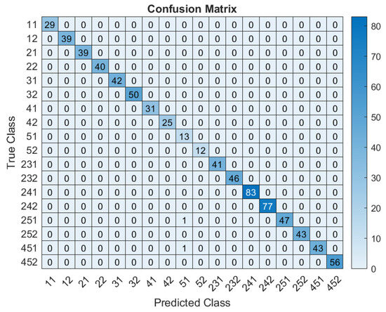
Figure 14.
YY-shaped wiring network, showing the confusion matrix for the validation phase.
To assess the classification performance, the Precision, Sensitivity, and F1-score metrics are computed separately for each class. As shown in Figure 15, the model consistently attains high values across all classes, demonstrating strong ability to reliably and robustly differentiate between various fault types.
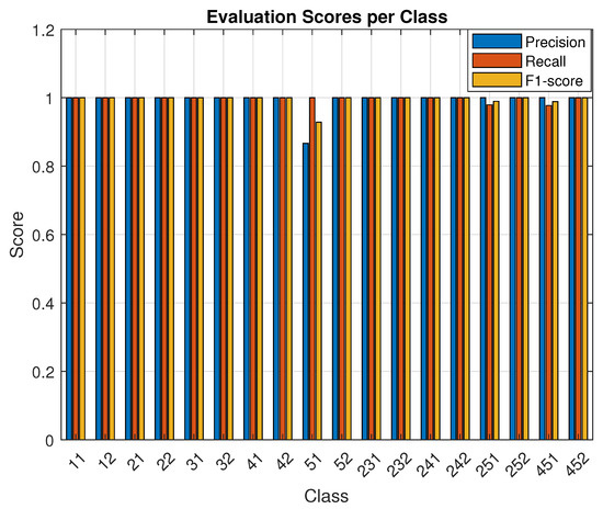
Figure 15.
Y-shaped wiring network, showing the evaluation metrics (Precision, Sensitivity, F1-Score) for each class i.
5.2.2. Online Monitoring
Next, we consider a YY-shaped wiring network in which a pair of specific branches are affected by a hard fault. Figure 16(top) illustrates the experimental situation where two hard faults occur on branches L2 and L5. To demonstrate the consequences of these faults, Figure 16(bottom) offers a comparative analysis between the experimentally obtained TDR response of the faulty network and the TDR response of the healthy network obtained using the forward model.
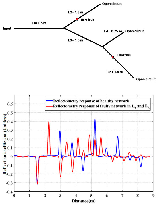
Figure 16.
(Top) Experimental scenario involving two hard faults on branches and ; (Bottom) TDR responses of the healthy and faulty YY-shaped wiring networks.
Following the approach adopted in the previous experiment, the diagnostic process for the YY-shaped wiring network begins with the calculation of the RMSE metric between the experimentally obtained TDR response of the faulty network and the simulated TDR response of the healthy network. The RMSE value confirms that the network under test is defective. As a result, the algorithm advances to the localization and characterization phases. The BiLSTM classifier model previously developed and validated during offline modeling is employed to identify the faulty branches. This model takes the experimental TDR response as input and outputs the class label associated with the affected branches. In this case, the classifier predicts Class 251, indicating that branches L2 and L5 are faulty due to open circuit-type faults. Subsequently, the BiLSTM regressor model is utilized to estimate the updated lengths of branches L2 and L5. The predicted faults are found to be located 0.37 meters along branch L2 and 0.38 meters along branch L5. The reconstructed wiring network is illustrated in Figure 17.

Figure 17.
The reconstructed YY-shaped network.
6. Conclusions
In this study, we have introduced a novel fault diagnosis framework that combines BiLSTM networks with TDR responses for improved detection, characterization, and localization of wiring faults. The proposed methodology begins by generating a detailed dataset through a forward model that simulates TDR responses across various fault scenarios and network topologies. This dataset is used to train BiLSTM-based classifiers and regressors that can capture long-term dependencies in both forward and backward signal directions. After training, the BiLSTM models are applied to unseen TDR responses for accurate fault diagnosis and localization. The proposed approach offers numerous benefits, including real-time diagnostics, adaptability to different wiring configurations, and avoidance of manual feature extraction or preprocessing requirements. Moreover, our approach promotes sustainable engineering practices by facilitating predictive and condition-based maintenance, helping to reduce unplanned system downtime, minimize resource-intensive diagnostic efforts, and extend the operational lifespan of wiring infrastructure. Experimental results validate our method’s effectiveness, demonstrating superior diagnostic accuracy and sensitivity compared to conventional techniques. Future work will focus on extending the proposed approach to diagnose network topologies affected by soft faults, address the diagnosis of faults in wiring networks under varying environmental conditions, and incorporate the evaluation of uncertainty in the diagnostic process.
Author Contributions
Conceptualization, A.G. and M.K.S.; methodology, A.G., M.K.S. and M.N.; software, A.G., M.K.S. and M.N.; validation, A.G., M.K.S. and M.N.; writing—original draft preparation, A.G.; writing—review and editing, M.K.S. and M.N.; funding acquisition, M.N. All authors have read and agreed to the published version of the manuscript.
Funding
This research work was funded by Umm Al-Qura University, Saudi Arabia under grant number 25UQU4300346GSSR16.
Informed Consent Statement
Not applicable.
Data Availability Statement
The data used during this study are available from the corresponding author upon reasonable request.
Acknowledgments
The authors extend their appreciation to Umm Al-Qura University, Saudi Arabia for funding this research work under grant number 25UQU4300346GSSR16.
Conflicts of Interest
The authors declare that they have no conflicts of interest.
References
- Furse, C.; Chung, Y.; Lo, C.; Pendayala, P. A critical comparison of reflectometry methods for location of wiring faults. Smart Struct. Syst. 2006, 2, 25–46. [Google Scholar] [CrossRef]
- Qinghai, S.; Kanoun, O. Model-based identification of wire network topology. Measurement 2014, 55, 206–211. [Google Scholar]
- Gao, Z.; Cecati, C.; Ding, S. A survey of fault diagnosis and fault-tolerant techniques—Part I: Fault diagnosis with model-based and signal-based approaches. IEEE Trans. Ind. Electron. 2015, 62, 3757–3767. [Google Scholar] [CrossRef]
- Hassen, W.; Auzanneau, F.; Peres, F.; Tchangani, A. A distributed diagnosis strategy using bayesian network for complex wiring networks. IFAC Proc. Vol. 2012, 45, 42–47. [Google Scholar] [CrossRef]
- Furse, C.; Kafal, M.; Razzaghi, R.; Shin, Y.J. Fault diagnosis for electrical systems and power networks: A review. IEEE Sens. J. 2020, 21, 888–906. [Google Scholar] [CrossRef]
- Furse, C.; Haupt, R. Down to the wire: Aging, brittle wiring within aircraft poses a hidden hazard that emerging technologies aim to address. IEEE Spectr. 2001, 28, 34–39. [Google Scholar] [CrossRef]
- Reis, J.D.; Castro, A.L.S.; Costa, J.C.W.A.; Rius, J.R.; Ericson, K. Sequence and spread spectrum time domain reflectometry for transmission line analysis. In Proceedings of the Broadband Access Communication Technologies II, Boston, MA, USA, 10–11 September 2007; Volume 6776, pp. 156–166. [Google Scholar]
- Lelong, A.; Carrion, M. On line wire diagnosis using multicarrier time domain reflectometry for fault location. In Proceedings of the SENSORS, 2009 IEEE, Canterbury, New Zealand, 25–28 October 2009; pp. 751–754. [Google Scholar]
- Qu, S.; Xu, Y.; Huang, S.; Sun, M.; Wang, C.; Shang, Y. Recent advancements in optical frequency-domain reflectometry: A review. IEEE Sens. J. 2022, 23, 1707–1723. [Google Scholar] [CrossRef]
- Dhamija, H. Optical Sequence Time Domain Reflectometry for Aircraft Wire Fault Location; University of Utah: Salt Lake City, UT, USA, 2010. [Google Scholar]
- Shi, Y.J. Theory and Application of Time-Frequency Analysis to Transient Phenomena in Electric Power and Other Physical Systems; The University of Texas at Austin: Austin, TX, USA, 2004. [Google Scholar]
- Ureña, F.; Gavete, L.; Benito, J.; García, A.; Vargas, A. Solving the telegraph equation in 2-D and 3-D using generalized finite difference method (GFDM). Eng. Anal. Bound. Elem. 2020, 112, 13–24. [Google Scholar] [CrossRef]
- Cheng, J.; Zhang, Y.; Yun, H.; Wang, L.; Taylor, N. A Study of Frequency Domain Reflectometry Technique for High-Voltage Rotating Machine Winding Condition Assessment. Machines 2023, 11, 883. [Google Scholar] [CrossRef]
- Chilan, M.; Pirhadi, A.; Asadi, S.; Helfert, S. Analysis of multiconductor transmission lines using the time domain method of lines. AEU-Int. J. Electron. Commun. 2021, 138, 153863. [Google Scholar] [CrossRef]
- Honarbakhsh, B.; Asadi, S. Analysis of multiconductor transmission lines using the CN-FDTD method. IEEE Trans. Electromagn. Compat. 2017, 1, 184–192. [Google Scholar] [CrossRef]
- Paul, C.R. Analysis of Multiconductor Transmission Lines; John Wiley & Sons: Hoboken, NJ, USA, 2007. [Google Scholar]
- Osman, O.; Sallem, S.; Sommervogel, L.; Carrion, M.; Bonnet, P.; Paladian, F. Distributed reflectometry for soft fault identification in wired networks using neural network and genetic algorithm. IEEE Sens. J. 2020, 20, 4850–4858. [Google Scholar] [CrossRef]
- Zhang, L.; Zhao, Z.; Zhang, D.; Luo, C.; Li, C. Particle swarm optimization pattern recognition neural network for transmission lines faults classification. Intell. Data Anal. 2022, 26, 189–203. [Google Scholar] [CrossRef]
- Chang, S.; Park, J. Wire mismatch detection using a convolutional neural network and fault localization based on time–frequency-domain reflectometry. IEEE Trans. Ind. Electron. 2018, 66, 2102–2110. [Google Scholar] [CrossRef]
- Smail, M.; Boubezoul, A.; Bouchekara, H.; Sellami, Y. Wiring networks diagnosis using time-domain reflectometry and support vector machines. IET Sci. Meas. Technol. 2020, 14, 220–224. [Google Scholar] [CrossRef]
- Banerjee, R.; Jamshed, A.; Haque, N. Localization of Faults in Coaxial Cables using Time-Domain Reflectometry and Support Vector Machine. In Proceedings of the 2023 IEEE 3rd Applied Signal Processing Conference (ASPCON), Haldia, India, 24–25 November 2023; pp. 242–245. [Google Scholar]
- Goudjil, A.; Smail, M. Wiring Network Diagnosis Using Reflectometry and Twin Support Vector Machines. Sustainability 2025, 17, 1836. [Google Scholar] [CrossRef]
- Smail, M.; Sellami, Y.; Bouchekara, H.; Boubezoul, A. Wiring Diagnosis using Time Domain Reflectometry and Random Forest. In Proceedings of the 2019 22nd International Conference on the Computation of Electromagnetic Fields (COMPUMAG), Paris, France, 15–19 July 2019; pp. 1–4. [Google Scholar]
- Goudjil, A.; Smail, M.; Pichon, L.; Bouchekara, H.; Javaid, M. Wiring networks diagnosis using K-Nearest neighbour classifier and dynamic time warping. Nondestruct. Test. Eval. 2024, 39, 2888–2905. [Google Scholar] [CrossRef]
- Goudjil, A.; Smail, M.K.; Bouchekara, H.; Pichon, L.; Pouliquen, M. A novel approach to wiring network diagnosis utilizing time domain reflectometry and one-dimensional convolutional neural networks. Neural Comput. Appl. 2025, 37, 15423–15445. [Google Scholar] [CrossRef]
- Smail, M.; Pichon, L.; Olivas, M.; Auzanneau, F.; Lambert, M. Detection of defects in wiring networks using time domain reflectometry. IEEE Trans. Magn. 2010, 46, 2998–3001. [Google Scholar] [CrossRef]
- Yao, J.; Yuan, B. Optimization Strategies for Deep Learning Models in Natural Language Processing. J. Theory Pract. Eng. Sci. 2024, 4, 80–87. [Google Scholar] [CrossRef]
- Oruh, J.; Viriri, S.; Adegun, A. Long short-term memory recurrent neural network for automatic speech recognition. IEEE Access 2022, 10, 30069–30079. [Google Scholar] [CrossRef]
- Abotaleb, M.; Dutta, P. Optimizing bidirectional long short-term memory networks for univariate time series forecasting: A comprehensive guide. Hybrid Inf. Syst.-Non-Linear Optim. Strateg. Artif. Intell. 2024, 443. [Google Scholar] [CrossRef]
- Han, T.; Ma, R.; Zheng, J. Combination bidirectional long short-term memory and capsule network for rotating machinery fault diagnosis. Measurement 2021, 176, 109208. [Google Scholar] [CrossRef]
- Han, Y.; Ding, N.; Geng, Z.; Wang, Z.; Chu, C. An optimized long short-term memory network based fault diagnosis model for chemical processes. J. Process Control 2020, 92, 161–168. [Google Scholar] [CrossRef]
- Lei, J.; Liu, C.; Jiang, D. Fault diagnosis of wind turbine based on Long Short-term memory networks. Renew. Energy 2019, 133, 422–432. [Google Scholar] [CrossRef]
- Appiah, A.; Zhang, X.; Ayawli, B.; Kyeremeh, F. Long short-term memory networks based automatic feature extraction for photovoltaic array fault diagnosis. IEEE Access 2019, 7, 30089–30101. [Google Scholar] [CrossRef]
- Saadi, M.; Bouteraa, N.; Redjati, A.; Boughazi, M. A novel method for bearing fault diagnosis based on BiLSTM neural networks. Int. J. Adv. Manuf. Technol. 2023, 125, 1477–1492. [Google Scholar]
- Hassan, S.; Zahid, M.M.; Abdullah, T.; Husain, K. Classification of cardiac arrhythmia using a convolutional neural network and bi-directional long short-term memory. Digit. Health 2022, 8, 20552076221102766. [Google Scholar] [CrossRef]
Disclaimer/Publisher’s Note: The statements, opinions and data contained in all publications are solely those of the individual author(s) and contributor(s) and not of MDPI and/or the editor(s). MDPI and/or the editor(s) disclaim responsibility for any injury to people or property resulting from any ideas, methods, instructions or products referred to in the content. |
© 2025 by the authors. Licensee MDPI, Basel, Switzerland. This article is an open access article distributed under the terms and conditions of the Creative Commons Attribution (CC BY) license (https://creativecommons.org/licenses/by/4.0/).