Article

Comparative Analysis of Supervised Machine Learning Algorithms for Forest Habitat Mapping in Cyprus

by
Maria Prodromou
1,2,*,
Ioannis Gitas
3,
Christodoulos Mettas
1,2,
Marios Tzouvaras
1,2,
Chris Danezis
1,2 and
Diofantos Hadjimitsis
1,2
1
ERATOSTHENES Centre of Excellence, Limassol 3012, Cyprus
2
Remote Sensing and GeoEnvironment Laboratory, Department of Civil Engineering and Geomatics, Cyprus University of Technology, Limassol 3036, Cyprus
3
Laboratory of Forest Management and Remote Sensing, School of Forestry and Natural Environment, Aristotle University of Thessaloniki, 54124 Thessaloniki, Greece
*
Author to whom correspondence should be addressed.
Sustainability 2025, 17(13), 6021; https://doi.org/10.3390/su17136021
Submission received: 2 May 2025 / Revised: 8 June 2025 / Accepted: 27 June 2025 / Published: 30 June 2025
(This article belongs to the Section Sustainable Forestry)

Abstract

Mapping dominant forest habitats is essential for guiding reforestation practices, especially in areas affected by fires. This study focuses on identifying dominant forest habitats in selected forested areas in Cyprus using supervised, pixel-based classification algorithms to support the planning of post-fire reforestation actions. For this study, three classifiers were provided by the Google Earth Engine (GEE) platform. Specifically, the Random Forest (RF), Support Vector Machine (SVM), and Classification and Regression Trees (CART) were implemented utilizing Sentinel-1 and Sentinel-2 data as well as topographic features and the tree density. Eight dominant forest habitats were mapped, including the Mediterranean pine forests with endemic Mesogean pines, Sarcopoterium spinosum phrygana, Thermo-Mediterranean and pre-desert scrub, Olea and Ceratonia forests, scrub and low forest vegetation with Quercus alnifolia, endemic forests with Juniperus, Cedrus brevifolia forests and Mediterranean pine forests with endemic Mesogean pines. The results revealed that RF and SVM outperformed CART. While SVM achieved the highest overall accuracy (OA) of 84.67%, it exhibited sensitivity to hyperparameter adjustments. In contrast, RF demonstrated greater stability and generalization across habitat types, attaining a reliable OA of 82.24%, making it the preferred classifier for this study.

1. Introduction

Mediterranean forests are a key component, known for their rich biodiversity and the wide range of environmental services they provide, including carbon sequestration, biodiversity conservation, and climate regulation [1,2]. Despite their recognized immense importance, these forests face increasing threats from climate change manifested through increased wildfire frequency, prolonged droughts, and extreme weather events [1,3]. As a result, these disturbances contribute to widespread ecosystem degradation, altering species composition and reducing forest resilience [3,4].
Focusing on the coniferous tree species found in Mediterranean ecosystems, common genera include Abies, Cedrus, Cupressus, Juniperus, Pinus, and Tetraclinis. Among Mediterranean forests, coniferous stands dominated by Pinus species are particularly significant yet vulnerable [4,5,6]. The genus Pinus includes four key Mediterranean-adapted species, Pinus brutia, Pinus halepensis, Pinus pinaster, and Pinus pinea [7,8] which cover approximately 16% of the region’s forest area [6]. Among them, Pinus brutia Ten., which is ecologically dominant in the eastern Mediterranean, comprises 90% of Cyprus’s forest cover (175,000 ha) due to its exceptional adaptability to arid conditions [9,10,11,12]. Nevertheless, its post-fire regeneration success can vary significantly depending on species and environmental context, underlining the need for precise habitat mapping to guide restoration efforts [13,14,15,16].
Traditionally, habitat identification relied on field surveys and manual observations [17]. While these methods provide valuable and direct measurements, their use is limited when monitoring at large scales. Consequently, forest monitoring has progressed to remote sensing (space and airborne). The need for more efficient and large-scale monitoring led to the development of aerial photography in the mid-20th century [18] and later to the development of satellite technology in the late 20th century, which significantly advanced forest habitat classification [19]. Advances in remote sensing have revolutionized forest monitoring through multi-sensor approaches that integrate optical (multispectral and hyperspectral) [20,21,22], Synthetic Aperture Radar (SAR) [23,24,25], and Light Detection and Ranging (LiDAR) data [26,27] as well as their fusion [23,28,29,30], which enables the capture of images across various spectral bands.
These technological developments have been complemented by machine learning techniques. According to the literature, various methods are described for plant classification utilizing earth observation data, with the choice of technique often determined by the specific objectives of the research. The selection of the algorithm significantly affects the classification performance due to the fact that each algorithm has its limitations and strengths [31]. Specifically, image classification algorithms differ in terms of complexity and their rationale. They can be categorized into two main categories: unsupervised algorithms like K-means and ISODATA and the supervised techniques that include Random Forest (RF), Support Vector Machines (SVMs), and neural networks [32,33]. The supervised pixel-based non-parametric models, such as SVM [34,35,36,37,38,39,40] and RF [32,41,42,43,44,45,46], have been widely adopted due to their robustness and high performance in remote sensing applications. Comparative studies have demonstrated the superior accuracy of RF over the classifiers, including SVM, Gradient Tree Boost, and Classification and Regression Trees (CART) [47,48,49,50,51], due to its ability to manage high-dimensional, noisy, and multi-source datasets, as well as its enhanced processing speed through efficient variable selection [44,52]. Moreover, in recent years, progress in machine learning has led to the development of deep learning methods for classifying plant species, including Convolutional Neural Networks (CNNs) [53,54,55,56], Long short-term memory Networks (LSTMs) [57,58], Recurrent Neural Networks (RNNs) [59,60], and Multilayer Perceptrons (MLPs) [61,62]. These methods have shown promising results in complex classification tasks and can capture spatial and temporal dependencies in the data. However, their implementation in forest habitat mapping using satellite imagery is limited due to their high computational demands, large data requirements, and the need for extensive labeled training samples, which are often unavailable in ecological studies [63,64].
Moreover, cloud computing platforms, such as Google Earth Engine (GEE), have brought significant advancements in forest habitat classification [65]. GEE has been widely used due to its capability to manage large datasets and execute complex analyses, offering state-of-the-art, pixel-based classification methods which are suitable for forest habitat classification in a variety of complex ecosystems [60,66,67,68]. According to the literature, several studies have been conducted to support the forest sciences [69], particularly in forest habitat classification using machine learning algorithms through the GEE platform. For instance, a study was conducted in Aspromonte National Park, in the south of Italy, using the Classification and Regression Trees (CART) algorithm for mapping forestry vegetation types [70]. Also, another study was conducted in Cyprus to map the dominant habitats in NATURA2000 regions using the Random Forest classifier [28]. Moreover, a study that focuses on the optimization of the SVM algorithm for argan tree classification using Sentinel-2 data in the Sous-Massa Region in Morocco was also conducted utilizing the GEE platform [71]. Also, Kaplan et al., 2020 [67] used the SVM algorithm to discriminate between broadleaved and coniferous forests with 94% accuracy. A comparative analysis for the identification of apicultural plants at Limnos island based on UAV multispectral imagery was also conducted by Papachristoforou et al., 2023 [66] showing that RF achieved the highest accuracy of 98.3% compared to Gradient Tree Boost, Classification and Regression Trees, Mahalanobis Minimum Distance, and Support Vector Machine.
Despite these advancements, significant challenges remain in habitat classification, including the discrimination between habitats with similar spectral responses, the optimization of multisource data fusion, and the development of transferable classification frameworks across Mediterranean ecosystems. This study aims to address these challenges by systematically applying and optimizing well-established classifiers using the GEE, with the goal of achieving operational scalability and reproducibility in habitat mapping. Moreover, this study provides a detailed understanding of the relative strengths, limitations, and suitability of the RF, CART, and SVM classifiers for habitat classification. By identifying the most effective classification approach, this study supports the development of more accurate and scalable forest mapping, which is essential for conservation efforts and supports ecological monitoring in Mediterranean forest ecosystems.
This study addresses these challenges by developing an optimized habitat mapping framework for Pinus brutia in Cyprus, with a focus on wildfire-impacted regions such as Solea and Argaka. Specifically, it presents the first comparative evaluation of RF, SVM, and CART classifiers for habitat-level forest mapping in Cyprus, implemented in GEE. The novelty of this work lies in the integration of multisource datasets derived from Sentinel-2, Sentinel-1, spectral indices, topographic features, and tree density, and the implementation of a hyperparameter tuning to improve the classification performance.
This study aligns with EU biodiversity targets and builds upon prior work, which focused on prioritizing areas for post-fire restoration in Cyprus [72]. Also, this research focuses on identifying the most suitable classification algorithm, which will be fine-tuned through hyperparameter optimization to accurately identify the dominant habitats in the study area, using forest habitats listed under the EU Habitats Directive.
This framework helps improve both ecological understanding of Mediterranean forest ecosystems and practical forest management, especially in areas prone to fires. Additionally, this study provides critical tools for post-fire recovery planning, habitat selection for reforestation, habitat degradation assessment, and supporting policies linked to the EU biodiversity strategy up to 2030 [73], the European Green Deal [74], and the EU Natura restoration legislation [75]. By using remote sensing for restoration purposes, this study helps reduce the impacts of climate change and rising disturbance pressures on Mediterranean forests [76,77].

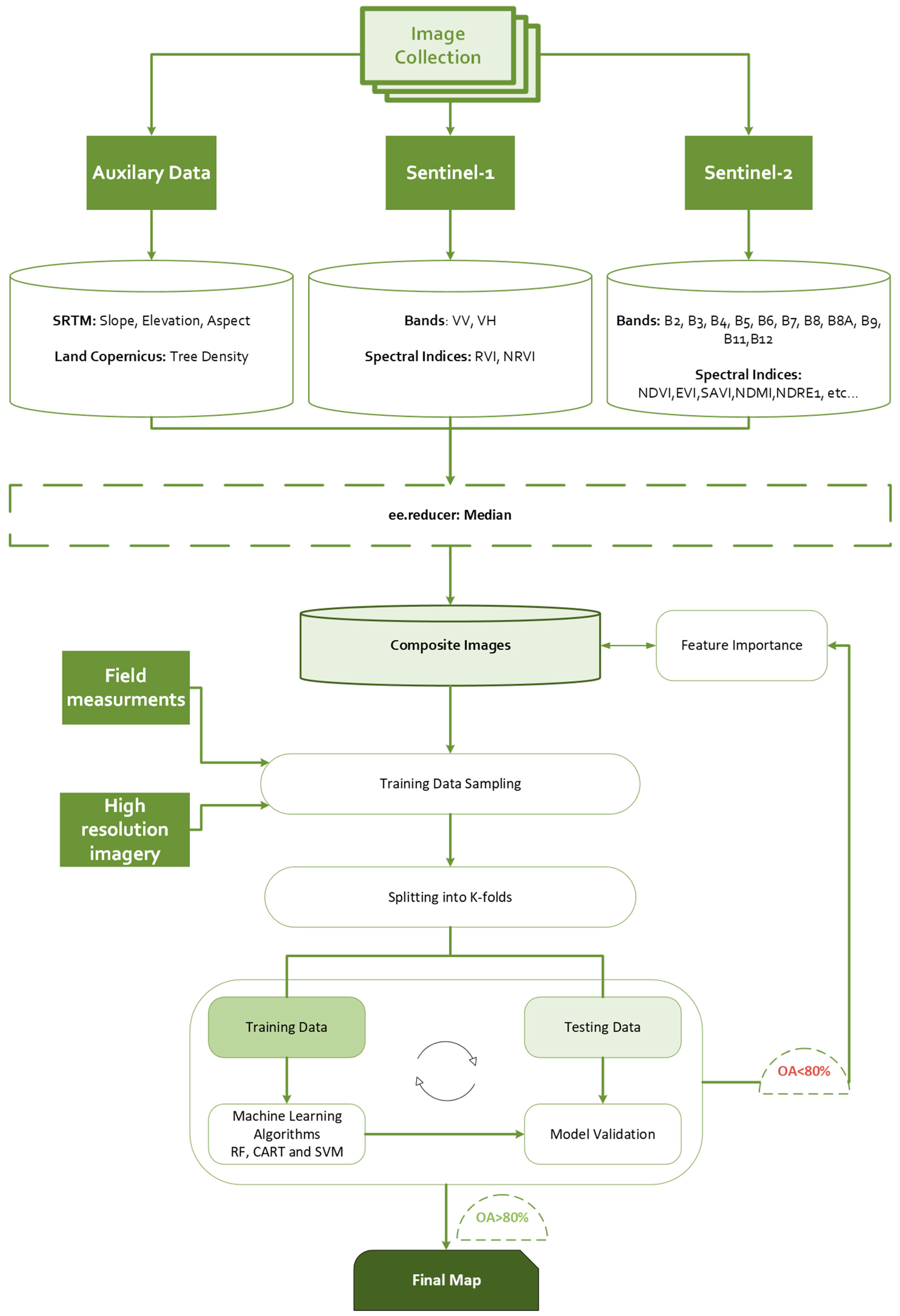
2. Materials and Methods

2.1. Study Area

The proposed methodology was implemented in selected forest areas of high importance in Cyprus, covering 2917 km2, as presented in Figure 1. Some characteristic areas included in the study area are the Pafos NATURA 2000 region, the Troodos UNESCO Geopark, Akamas Natura 2000 and the Lemesos Natura 2000 region, among others. The Troodos UNESCO Global Geopark is located in central Cyprus, characterized by its unique ophiolite geology and diverse ecosystems [78,79]. The area is also notable for its rich flora biodiversity, hosting the highest concentration of plant and endemic species on the island. Moreover, it has been recognized as one of the 13 “Plant Diversity Hot Spots” in the Mediterranean region [80]. Regarding the the Pafos State Forest located in the northwest part of the Troodos range, it is among the most significant state forests in Cyprus, distinguished for its high biodiversity and the presence of various plant and animal species. Additionally, as a Special Protection Area (SPA), it hosts 96 bird species. Notably, it is the only biotope in Cyprus where the endemic Ovis orientalis ophion can be found [81].
The Akamas peninsula, located in the western part of the island, holds considerable ecological importance due to its strategic location and diverse landscape position. It demonstrates well-preserved eastern Mediterranean ecosystems, characterized by diverse habitats and species. Notably, it is one of the only three peninsulas on the island hosting the endemic serpentinophilous grasslands. Akamas is also a key area for avifauna, particularly migratory birds, making it an important site for bird conservation [82].
Focusing on burned areas, two study areas were selected which are the fire events in Solea and Argaka. The fire in Solea village (Nicosia region), which occurred on 19 June 2016, had an estimated burned area of 18.85 km2, according to data from the Forest Department. It was one of the largest wildfires in the forest area in Cyprus during the last years. Similarly, the fire in Argaka area (Paphos region) erupted on 18 June 2016, with an estimated burned area of 7.63 km2. The predominant vegetation in these regions consists of Pinus brutia forests with an understory comprising herbaceous plants and shrubs. The climate in these areas is typical of the Mediterranean, characterized by hot, dry summers and mild, rainy winters. Additionally, the Solea burned area is distinguished by steep slopes, while the terrain in the Argaka area features mild to moderate slopes.

2.2. Methodology

The mapping of the primary forest habitats in the state forests of Cyprus was conducted using Sentinel-1 and Sentinel-2 satellite images, combined with auxiliary datasets such as tree density, elevation, slope, etc. Regarding the Sentinel-2 data, it is highlighted that, in this study, only the bands with 10 m and 20 m spatial resolution were used, and also, in order to avoid any impacts from the cloud cover in the analysis, the images were filtered to have less than 10% cloud percentage cover across the entire scene.
Topographical features were also incorporated, given that some habitats often exhibit different distribution patterns based on the elevation, aspect, and slope. For this purpose, elevation data from the Shuttle Radar Topography Mission (SRTM) at 30 m resolution were used. These topographical features provided the algorithm with additional information regarding distribution of habitats across varying terrains, enhancing classification performance.
Additionally, to account for variability in vegetation density across different habitats, the Land Copernicus High Resolution Layer Tree Cover Density product [83] in 20 m spatial resolution was utilized. The Tree Cover Density product derived from the Land Copernicus provides a quantitative measure of the density of tree canopy coverage in each pixel, expressed as a percentage (0–100%). Specifically, it presents the proportion of ground covered by tree crowns within a 10 m spatial resolution [84]. This dataset offered valuable information on the percentage of tree cover within the study area, further supporting the mapping process.
The image processing workflow, illustrated in Figure 2, was implemented using the GEE platform. Specifically, GEE enabled the extraction of band reflectance values and backscatter coefficients from Sentinel-2 and Sentinel-1 data, respectively, as well as the calculation of vegetation indices for the implementation of pixel-based machine learning classification algorithms, which were tested and compared to identify the classifier with the best performance for mapping the dominant forest habitats in Cyprus. Specifically, these datasets were combined using the median reduction to create composite images. Also, high-resolution imagery and field measurements were incorporated for ground truth validation. Additionally, k-folds were used for the validation of the model. Different machine learning algorithms were tested, and a feature-importance analysis was used to identify the key drivers. Moreover, the model’s performance was assessed using accuracy assessment metrics, and in cases where the overall accuracy achieved 80%, the model was used for the development of the final habitat map. A detailed description of each step in the proposed methodology is provided in the following sub-sections.

2.2.1. Training Samples Collection

To map the dominant habitats in Cyprus, we selected habitat types from groups 5 and 9, in accordance with the EU Habitats Directive, as outlined in Table 1. Specifically, the EU Habitats Directive categorizes natural environments into nine main groups: (1) forests, (2) natural and semi-natural grassland formations, (3) raised bogs and mires and fens, (4) temperate heath and scrub, (5) coastal sand dunes and inland dunes, (6) freshwater habitats, (7) rocky habitats and caves, (8) coastal and halophytic habitats, (9) sclerophyllous scrub [85].
The collection of the samples for the forest habitats was conducted through photo interpretation, a widely used method in classification studies using remote sensing techniques due to its cost-effectiveness and ability to leverage high-resolution reference imagery [86,87]. Specifically, high-resolution images from Google Earth and the georeferenced digital aerial ortho-photos provided by the Department of Lands and Surveys for the years 2014 and 2019 were used for photo interpretation, which are accessible as a base- map in ArcGIS Pro (version 3.0.3) software. The data were collected primarily to cover the forest areas of high importance in Cyprus. A total of 10,000 points were collected through this approach.

2.2.2. Variable Selection

The proposed methodology was implemented in two different datasets which are based on the variables used by Prodromou et al., 2024 [88] in their study about the Forest Habitat Mapping in Natura2000 regions in Cyprus using Random Forest, so for the purposes of this study, the dataset that achieved higher performance was selected. The other dataset enhances the abovementioned methodology and includes more spectral indices and the tree density [84] provided by Land Copernicus in the model.
As shown in Table 2, the first dataset includes 18 variables and the second dataset 40 variables. These combinations include the bands from each satellite sensor, the topographic features, and the spectral indices listed in Table 3, which were considered to determine the optimal parameters for forest habitats classification using machine learning. All variables used were normalized to a 0 to 1 range. The variable reduction process is important because it helps to minimize weak learners that generate weak outliers. Specifically, this method reduces the number of predictors, while increasing accuracy by eliminating irrelevant variables [89,90].
The spectral indices are formulas that primarily focus on band ratios or feature scaling techniques, such as normalized or standardized algorithms, which rely on the combination of pixel values from two or more spectral bands [91,92]. Their use relies on the sensitivity they offer in identifying certain features more effectively than individual spectral bands for spectral signature detection [91]. They are designed to highlight pixels in an image that shows a relative presence of a specific land cover as well as to emphasize the aspects of an ecosystem’s functionality, and they have contributed significantly to a more comprehensive understanding of environments and ecosystems in space and time [92,93].
Spectral indices are generally categorized based on the type of remote sensing platform used to acquire the data, distinguishing between airborne and satellite-based systems [92]. In the context of this study, which focuses on passive satellite remote sensing, spectral indices are further classified according to the spectral bands they utilize. These include indices derived from simple ratios, as well as those combining bands from the visible part of the spectrum with near-infrared (VNIR), red edge, mid-infrared, and shortwave infrared (SWIR) regions of the electromagnetic spectrum [92].
Spectral indices have been developed for a wide range of applications. For this study, we calculated indices related to vegetation health, moisture content, and burned area detection. Table 3 summarizes the spectral indices employed to assess the spectral responses of forest habitats, using commonly applied indices derived from Sentinel-1 and Sentinel-2 data.
Each index contributes specific insights to the analysis. For instance, the Normalized Difference Vegetation Index (NDVI) is widely used to assess vegetation health [94], while the Soil-Adjusted Vegetation Index (SAVI) compensates for soil brightness effects in areas with sparse vegetation. To assess leaf water content, the Normalized Difference Moisture Index (NDMI) was applied, which is based on the ratio of near-infrared (NIR) to shortwave infrared (SWIR) reflectance [95]. The Normalized Difference Red Edge Index (NDRE), a variant of NDVI that substitutes the red band with the red edge band, was also utilized [96]. For detecting fire disturbances and mapping burn scars, the Normalized Burn Ratio (NBR) was applied, as it is one of the most widely used indices for this purpose [97,98]. NBR is calculated using the difference and sum of NIR and SWIR reflectance, corresponding to bands 8 and 12 of the Sentinel-2 sensor, respectively. The Normalized Burn Ratio (NBR) ranges from −1 to +1, where lower values typically indicate bare soil or recently burned areas, while higher values correspond to healthy or unburned vegetation. A variation of this index, known as NBRSWIR, uses the SWIR1 and SWIR2 bands instead. This modified version also includes two constants: a subtraction of 0.02 to normalize water-related changes toward zero or negative values, and an addition of 0.1 to mitigate the effect of anomalous water changes [99].
Another related index, NBRplus, is specifically designed to account for water reflectance and also ranges from −1 to +1, with higher values indicating burned areas [100]. The BAI is designed to highlight burned areas, focusing on the charcoal spectral signature in post-fire images within the red to near-infrared spectrum. Specifically, the index is determined using the red to near-infrared spectrum. Specifically, the index is determined by calculating the spectral distance of each pixel in relation to a reference point as a result burned areas represented by brighter pixels [101]. Furthermore, the BAIS2 is a modification of the BAI to suit the S2 bands including the visible, red edge, NIR, and SWIR bands. The values of the BAIS2 range from −1 to +1 for the identification of burn scars and from 1 to 6 in cases of active fires. The CSI is designed to detect the signals of black carbon in order to estimate the fire severity and is determined by the ratio of NIR and SWIR2 spectral bands [102]. The MIRBI index demonstrates significant effectiveness in distinguishing between burned and unburned areas [103].
Regarding the spectral indices of the Sentinel-1 data, the NDPI was selected because it provides information on the surface roughness [104], while the RVI is considered more suitable for vegetation monitoring due to its lower sensitivity to environmental factors such as soil moisture [105].
Through this way, the objective is to identify the most effective combination of spectral bands and indices to improve the performance of machine learning algorithms. Based on the wide range of literature, several studies have shown that integrating SAR and optical data helps capture distinct physical and spectral characteristics of land cover, thereby potentially improving classification results [106,107,108,109,110]. Furthermore, many other studies have confirmed that the use of spectral indices contributes to greater classification accuracy [88,111,112].
Table 3. Spectral indices equations based on S2 and S1, which are used in Datasets 1 and 2.
SatelliteSpectral
Indices
AbbreviationEquationRef.
S2Normalized Difference Vegetation IndexNDVI N I R R E D N I R + R E D [94]
Normalized Difference Red Edge IndexNDRE N I R R E D N I R + R E D [113]
Enhanced Vegetation IndexEVI 2.5 ( N I R R E D )   N I R + 6   R E D 7.5 B L U E + 1 [114]
Green Leaf IndexGLI 2 × G R E E N R E D B L U E 2 × G R E E N + R E D + B L U E [115]
SAVISAVI 1.5 ( N I R R E D )   N I R + R E D + 0.5
Structure Insensitive Pigment IndexSIPI N I R B L U E N I R R E D [116]
Atmospherically Resistant Vegetation IndexARVI N I R ( 2 × R E D ) + B L U E N I R + ( 2 × R E D ) + B L U E [117]
Bare Soil IndexBSI (   S W I R 1 + R E D ) ( N I R + B L U E ) S W I R 1 + R E D   + ( N I R + B L U E ) [118]
Normalized Difference Water IndexNDWI G R E E N N I R G R E E N + N I R [119]
Advanced Vegetation IndexAVI N I R 1 R E D × ( N I R R E D ) 3 [120]
Green Normalized Difference Vegetation IndexGNDVI N I R G R E E N N I R + G R E E N [113]
Normalized Difference Moisture IndexNDMI S W I R N I R S W I R + N I R [95]
Normalized Burn RatioNBR N I R S W I R 2 N I R + S W I R 2 [98]
Burned Area IndexBAI 1 ( 0.1 R E D 2 + 0.06 N I R 2 ) [101]
Burned Area Index for Sentinel 2BAIS2 1 R E 2 × R E 3 × N I R n G R E E N B 4 × ( S W I R 2 N I R n S W I R 2 + N I R n + 1 ) [121]
Char Soil IndexCSI N I R S W I R 2 [102]
Mid-Infrared Burn IndexMIRBI 10   ×   S W I R 2 9.8 × S W I R 1 + 2 [103]
Normalized Burn Ratio SWIRNBRSWIR S W I R 2 S W I R 1 0.02 S W I R 2 + S W I R 1 + 0.1 [99]
Normalized Burn Ratio PlusNBRplus S W I R 2 N I R n G R E E N B L U E S W I R 2 + N I R n + G R E E N + B L U E [100]
S1Radar Vegetation IndexRVI 4 V H V H + V V [122]
Normalized Difference Polarization IndexNDPI V V V H V V + V H [123]

2.3. Machine Learning Algorithms

The Google Earth Engine (GEE) platform includes a classifier package that enables supervised classification using several conventional machine learning algorithms. In this study, we evaluated the performance of three commonly used classifiers: Random Forest (RF), Classification and Regression Trees (CART), and Support Vector Machine (SVM). These algorithms were selected due to their proven reliability and effectiveness in forest habitat classification. A brief overview of each classifier is provided below.
CART is a non-parametric, tree-based algorithm rooted in fuzzy mathematical principles and is used to build predictive models. Introduced by Breiman in 1984 [124], CART constructs decision trees by recursively partitioning the data space and fitting classification or regression models to the resulting subsets. The algorithm continues to split the nodes until terminal nodes are reached. It is capable of handling both continuous and categorical variables and is valued for its simplicity, interpretability, and visualization. Moreover, CART uses surrogate splits to manage missing data efficiently, making it a versatile method for complex decision-making tasks [124].
RF algorithm is a tree-based ensemble learning method, where each prediction is influenced by a randomly sampled vector that follows the same distribution across all observations [125]. Unlike a single decision tree, RF aggregates the results of multiple decision trees using either averaging (for regression) or majority voting (for classification), which enhances predictive performance and reduces sensitivity to data variability and overfitting [126]. The model constructs decision rules at each internal node, starting from the root, and continues the splitting process until a stopping criterion is met [127].
SVM, developed by Cortes and Vapnik in 1995 [128], is a widely adopted classification algorithm. It works by identifying hyperplanes that best separate data into distinct classes. The optimal hyperplane is the one that maximizes the margin between the closest data points of each class, known as support vectors [129]. SVM is not limited to linearly separable datasets for non-linearly separable data; a kernel function is used to map the data into a higher-dimensional space where it can become linearly separable. SVM utilizes different types of kernel functions such as linear, polynomial, and radial basis function (RBF) and sigmoid. The most used kernels are polynomial and radial basis function kernels. For the purposes of this study, the RBF kernel was selected for its proven effectiveness compared to other studies [130].
Moreover, since many machine learning algorithms require the specification of hyperparameters, which can have a significant influence on the performance of the model depending on the dataset used, hyperparameter tuning for each classifier was also performed in this study [131]. The models were optimized utilizing the error matrix to identify the best parameter combinations and assess the model accuracy. Table 4 presents the hyperparameters and their corresponding values for each classifier used for the purposes of this study. Default parameters that were not modified are not included in this table.
It is highlighted that the identification of the optimal hyperparameters was conducted through the grid search method, where we examined how changes in the parameters (described in Table 4) influence the accuracy of the algorithms. Specifically, the grid search method requires a classifier to guide the process and a set of possible settings for the corresponding classifier, which it tests by every combination of these settings by training the classifier on the given dataset [132]. After that, it checks how well the classifier performs on separate test data using accuracy. This approach is implemented for the different training and testing splits, which, in our case, are based on the k-fold cross-validation as described in the following sub-section.
Table 4. Hyperparameter tuning per classifier.
ML
Algorithm
HyperparameterValueDescriptionSource
RF‘numTrees’50, 100, 500Corresponds to the number of decision trees to create.[124]
‘maxNodes’10, 30, 100Specifies the maximum number of leaf nodes in the decision tree. If not specified, there is no limit on the maximum number of nodes by default.
‘minLeafPopulation’1, 10, 50Determines the minimum number of data points needed to generate new nodes while building the decision tree. By default, this value is set to one.
CART‘maxNodes’10, 30, 100
‘minLeafPopulation’1, 10, 50
SVM‘kernelType’RBF:
(exp(−γ × |u − v|2))
RBF was selected for its effectiveness compared to the other kernels, better suitability to match the non-linear data characteristics, and widespread use [130]. The RBF is dependent on two important parameters, the cost (C) and gamma.[128,133]
‘cost’1, 10, 50, 100The C parameter is useful for managing the misclassification of training samples. When C is set to a higher value, it leads to a decrease in the number of misclassified training examples.
‘gamma’0.01, 0.1, 0.5, 1The gamma parameter controls the range of influence for the kernel. A lower gamma value indicates that a single training sample has a broader impact, whereas a higher gamma value leads to a more localized area [134].

2.4. Accuracy Assessment
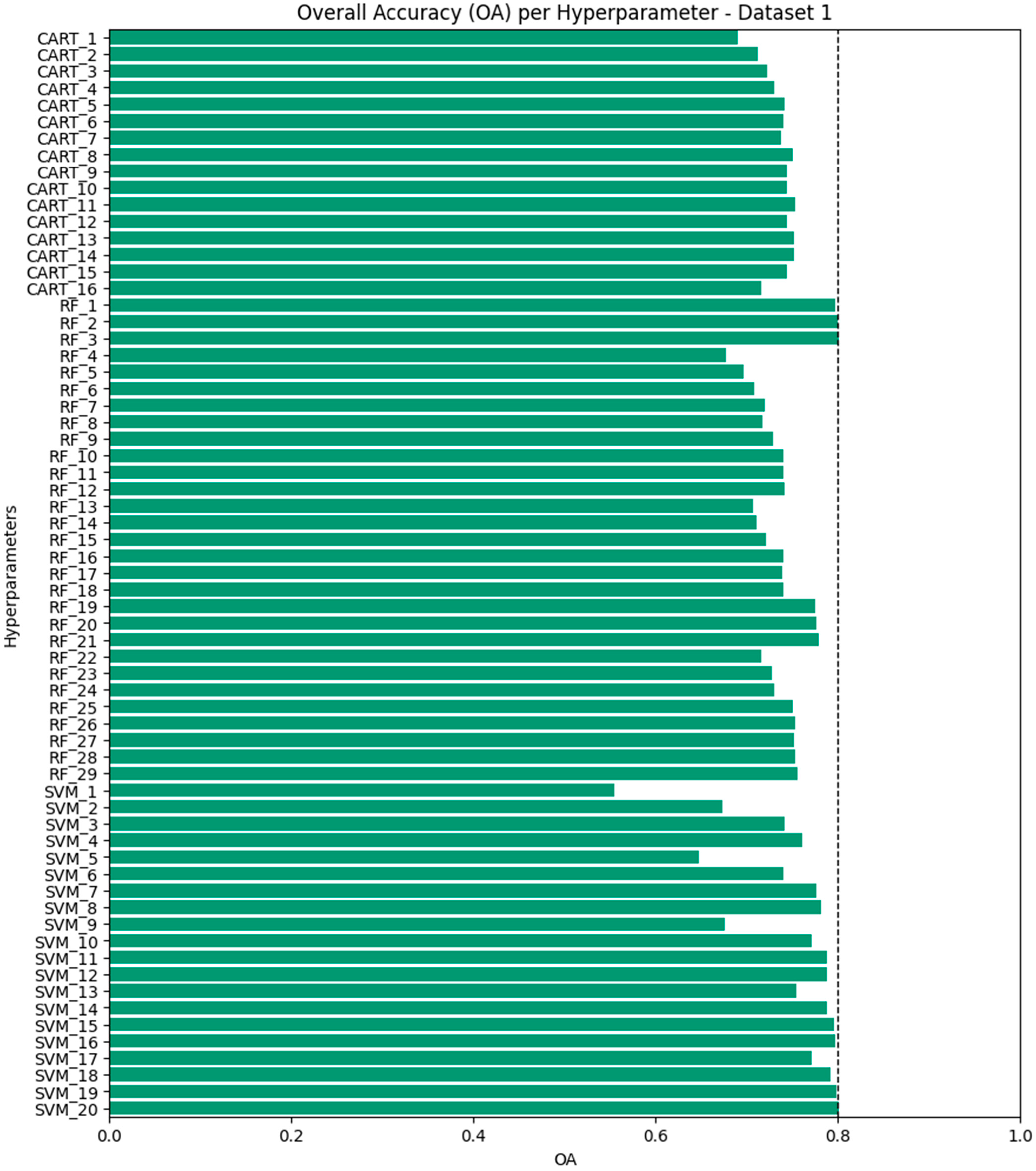
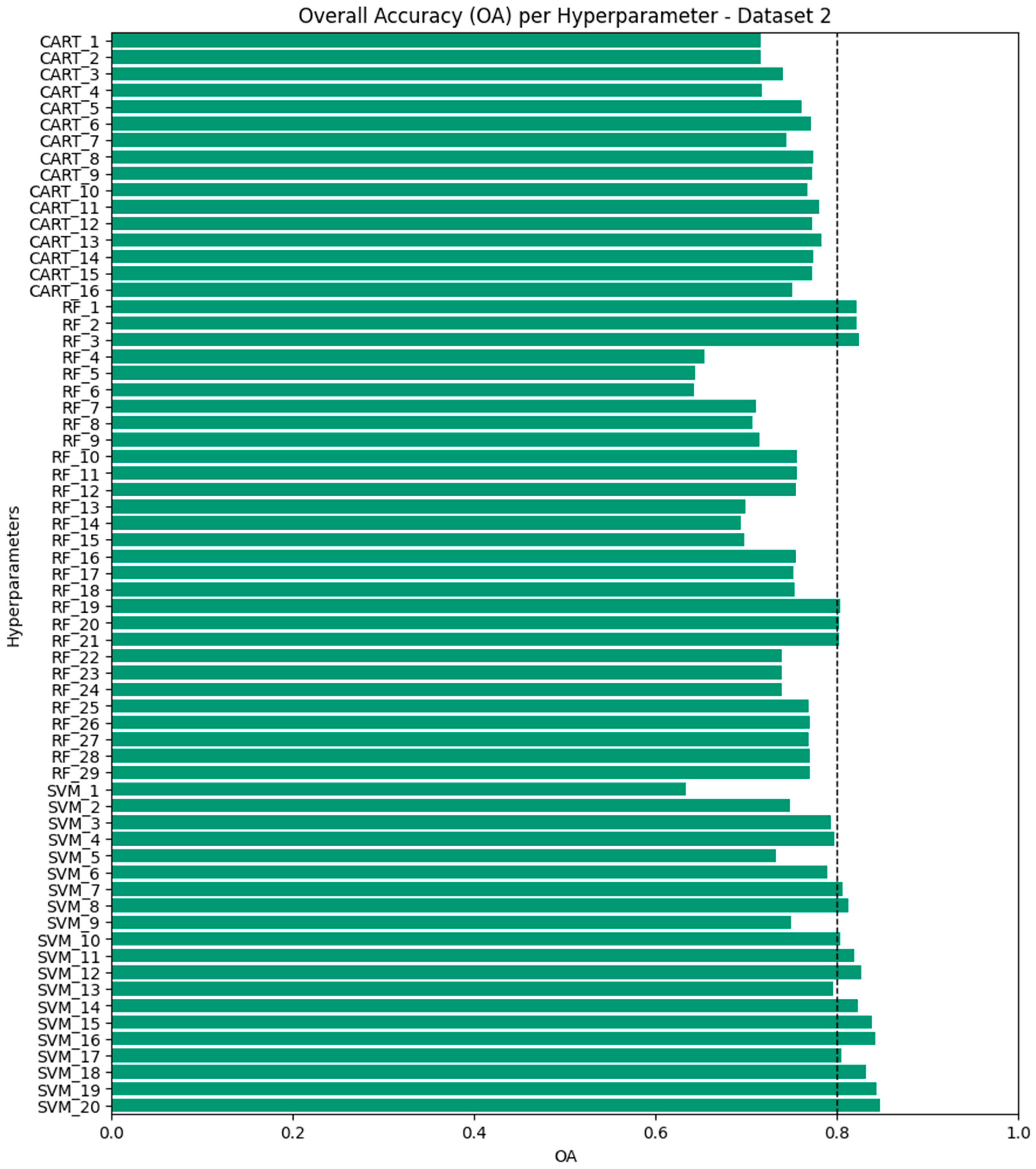
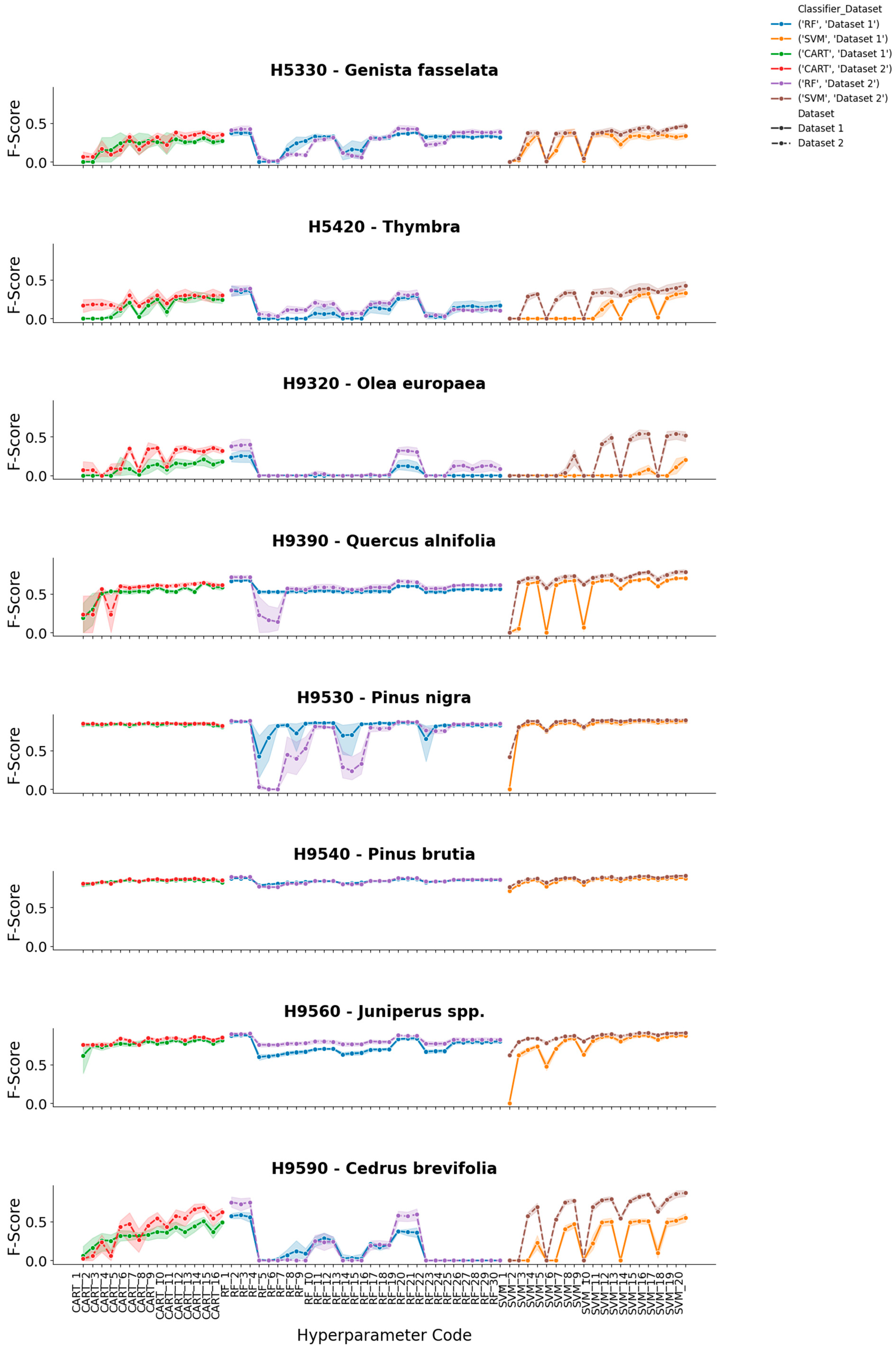
Accuracy assessment is essential for evaluating the performance of a classification algorithm. One of the most commonly applied statistical methods in land-cover classification is the confusion matrix. For each case study, the collected samples were divided into training and testing sets using a k-fold cross-validation approach. From the resulting confusion matrix, several key performance metrics were calculated, including the kappa coefficient, overall accuracy, producer’s accuracy, user’s accuracy, and the F1 score. Based on these metrics, the k-fold cross-validation was utilized. In k-fold, all the samples are divided into k groups of samples, called folds. The prediction function is learned using the k-1 folds, with the remaining fold used for the validation of the model [135,136]. The k is typically set to 5 or 10, as these values have been found to provide estimates that balance between high bias and high variance; however, there is no strict rule for determining the value of k [137,138]. For the purposes of this study, the stratified 5-fold cross-validation was conducted.
The confusion matrix compares the classified results to the ground truth data by thematic category. Overall accuracy indicates the proportion of pixels that were correctly labeled. Producer’s accuracy reflects how accurately the model identifies reference pixels for each class, while user’s accuracy shows the likelihood that a pixel classified into a specific category belongs to that true class, based on the reference sample [68,112,139]. The Kappa statistic evaluates classification performance relative to chance agreement and expresses the overall consistency between the classification and the ground truth [112]. It ranges from 0 to 1, where values near 0 suggest no agreement between the classified results and the reference (truth) data, and values near 1 indicate strong agreement between classified and reference (truth) data. The F-score, which combines recall and precision, offers an additional accuracy metric that balances user’s and producer’s accuracy [68].
O A = 1 N i = j = 1 n C i j ,
P A = C i j i = j = 1 n C j ,
U A = C i j i = j = 1 n C i ,
F = 2 P A U A P A + U A ,
K a p p a   C o e f f i c i e n t = N i = j = 1 n C i j i = j = 1 n C i C j N 2 i = j = 1 n C i C j
where N is the number of rows in the error matrix, Cij denotes the number of observations in both a specific row and column, Cj is the total number of observations in a column, N is the total number of observations, PA is producer’s accuracy, and UA is user’s accuracy.

3. Results

3.1. Classification Performance

This study examines the performance of three supervised pixel-based algorithms, namely RF, SVM, and CART, using the dataset proposed by Prodromou et al. [88] which includes Sentinel-2 imagery (spectral bands and vegetation indices) and topographical features (elevation, aspect, and slope) through the GEE. Apart from this, as a second dataset, a dataset that also incorporates additional spectral indices based on Sentinel-1 and Sentinel-2 and the tree density was used to identify the necessary habitats for reforestation actions for the Solea and Argaka fire events. For this purpose, an image composite for June 2016 was used in order to show the situation before the fire events. The selected study area was classified into eight dominant habitats which are the H5330—Genista fasselata, H5420—Thymbra, H9320—Olea europaea, H9390—Quercus alnifolia, H9560—Juniperus Spp., H9540—Pinus brutia, H9530—Pinus nigra, and H9590—Cedrus brevifolia. It is highlighted that, for both datasets, the same training and validation samples were used for each classifier.
Focusing on the identification of the dominant habitats in the highly important forest areas in Cyprus, Figure 3 and Figure 4 present the results of applying the RF, CART, and SVM algorithms using hyperparameter tuning for Dataset 1 and Dataset 2, respectively. In Appendix B, Figure A1 and Figure A2 present the results in the 5-fold cross-validation for each hyperparameter. The description of the codes used for each hyperparameter is presented in Appendix A in Table A1. The values in blue color represent high accuracy while the values in red colors indicate low OA. Moreover, values with an OA greater than 80% are marked (*). Through this approach, 30 experiments were conducted using RF, 20 using the SVM, and 16 using the CART algorithm for each fold. Obviously, the results present significant variations across the different classifiers in each hyperparameter tuning.
Based on the results derived from the hyperparameter tuning for Dataset 1, the RF classifier showed stable and relatively high performance in different hyperparameter configurations. Specifically, RF achieved OA values that ranged consistently between 67.67% and 80.03% and Kappa 0.37 to 0.67. As can be seen from the various combinations made with the grid search method, the best performance was achieved using a larger number of trees and nodes and keeping the remaining parameters at default values. Utilizing Dataset 2, the RF achieved OA values that ranged between 64.20% and 82.45% and Kappa 0.27 to 0.71. Based on the hyperparameter tuning, the best performance resulted using numTrees = 500 and the remaining parameters set as default without making ineffective the reliability of the other classifiers since they presented small differences in the results.
Regarding the SVM classifier, Dataset 1 presents wider variations in the OA ranging from 55.46 to 80.13%, and kappa values ranging from 0.00 to 0.67 across the different combinations of the hyperparameter. Specifically, the classifier presents lower OA in cases where the model used lower gamma, for instance, gamma = 0.01, leading to an OA equal to 55.45% (cost = 1, kernel = RBF, gamma = 0.01). In contrast, the model achieved higher OA in cases where higher cost and gamma values were used, achieving OA equal to 80% (cost = 100, kernel = RBF, gamma = 1). The classifier presents similar trends also in Dataset 2, but in this case, the results are improved; for example, the OA ranged from 63.29% (cost = 1, kernel = RBF, gamma = 0.01) to 84.67% (cost = 100, kernel = RBF, gamma = 1) and kappa ranged from 0.25 to 0.76.
Moreover, the CART algorithm in Dataset 1 exhibits moderate performance across different hyperparameters, with OA values typically ranging from 0.66 to 0.76. It is highlighted that in some cases, the CART model achieved similar performance with RF and SVM, but it did not achieve the highest performance achieved from SVM (OA = 80%). Taking into account the performance of the CART classifier suggests that this model cannot generalize as well as the RF and the SVM utilizing the dataset from Dataset 1 despite that, in some cases, it achieves competitive accuracy like the other classifiers. Also, when comparing the performance of each classifier based on the hyperparameters configurations utilizing Datasets 1 and 2 as shown in Figure 5, RF seems to have a high performance based on habitats such as H9530, H9540, and H9560, with the highest performances reaching F1-scores of 87% based on Dataset 1 and slightly higher ones with Dataset 2, at 88–89%. Habitats H9390 and H9530 exhibited a more moderate performance, with maximum values of 58.35% for H9390 and 67.24% for H9530, whereas Dataset 2 demonstrated better performance, with the highest values reaching 74.78% and 71.54%, respectively. In contrast, RF presents a weakness in the classification of habitats H5330, H5420, and H9320, which presented very low performances in F1-score values, with Dataset 2 presenting slightly higher performances.
SVM presented significant variations in its performances across the different hyperparameter configurations. However, habitats H9530, H9540, and H9560 still achieved the highest F1-scores, especially utilizing Dataset 2, with the highest F1-score values ranging from 89 to 90%, while in Dataset 1, from 86 to 87%. Regarding habitat H9590, it presented a substantial difference in its performance based on F1-score values based on the two datasets, since, based on Dataset 1, the performance was 54.87%. In contrast, with Dataset 2, the habitat was better identified with a maximum F1-score performance value reaching 86.71%, based on Dataset 2. The performance for habitat H9390 was similar in both datasets, with Dataset 2 showing slightly higher performance than Dataset 1. However, even in this case, the habitats H5330, H5420, and H9320 presented difficulty in their identification since the maximum performances based on the F1-score values ranged from 20.31 to 37.87% using Dataset 1 while Dataset 2 showed higher maximum values from 42.29 to 53.78%.
The CART algorithm exhibited a similar trend to RF and SVM in habitat identification, i.e., better performances in H9530, H9540, and H9560, moderate in H9590 and H9390, and very low in H5330, H5420, and H9320. However, the performance of CART based on F1-score consistently produced lower F1-scores compared to RF and SVM, indicating that it is a less effective classifier for habitats classification.

3.2. Selection of the Optimal Classifier

Comparing the three classifiers based on the abovementioned accuracy metrics (kappa, OA, and F1-score), the SVM utilizing the optimal hyperparameters achieves the highest accuracy, followed by RF, which has slight differences with SVM, while CART performed relatively lower utilizing Dataset 2. This approach has highlighted the importance of hyperparameter tuning for the optimization of classification performance, especially for SVM, which presents significant variations in the performance across the different parameter selections.
According to the analysis conducted in the previous section on forest habitat mapping, Dataset 2 improved the classification accuracy across all classifiers. Regarding the selection of the classifier, utilizing the SVM classifier with cost = 100, kernel = RBF, and gamma = 1, the model achieved the highest performance compared to the other classifiers. However, a high cost and gamma value can lead to overfitting.
So, in order to mitigate this issue, the decision on the optimal classifier was taken based on models and the used hyperparameters that achieved an OA higher than 80%. Consequently, for the purposes of this study, RF was selected as it provides high accuracy, slightly lower than SVM, but with better generalization. Specifically, RF (numTrees = 500) was selected for habitat mapping in the study area to avoid the risk of overfitting and ensure generalization. Moreover, this choice achieves competitive OA while maintaining consistent F1-scores across different classes and is also less sensitive to hyperparameter tuning in contrast with SVM, which requires careful tuning of cost and gamma, making it more prone to overfitting if it does not have the appropriate optimization.

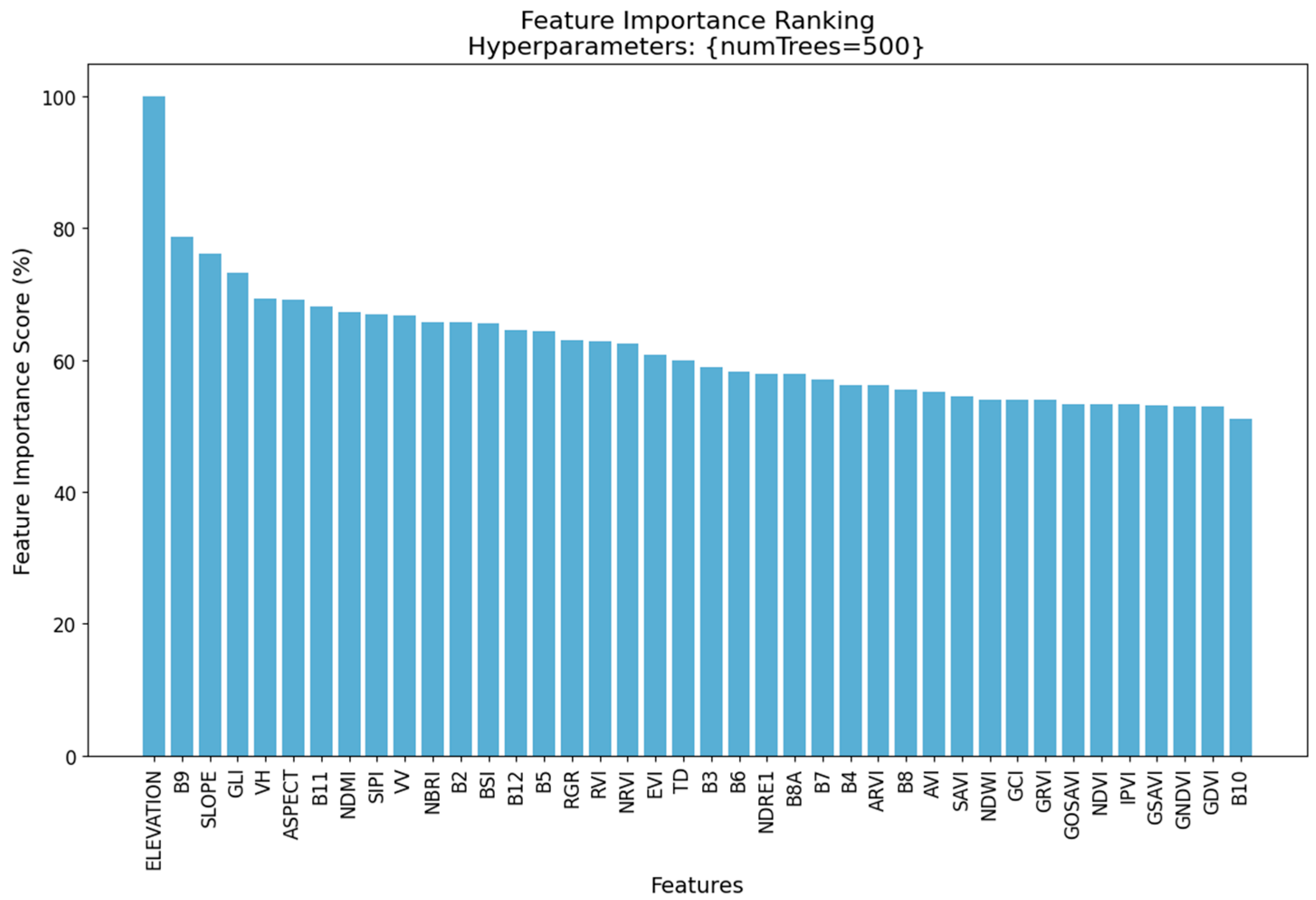
3.3. Feature Importance

Figure 6 presents the relative contribution of the input variables in forest habitats classification using the RF classifier based on the RF_3 hyperparameter based on Dataset 2. Among the predictors, elevation was identified as the most influential variable, underscoring the strong relationship between forest habitats distribution and topographic variations. Other top-ranked terrain-related variables, such as the slope and the aspect, also contributed significantly to classification accuracy, ranking within the top five most important variables.
Among the Sentinel-2 spectral bands, B9 (water vapor absorption band) had a high importance score, indicating its relevance in distinguishing forest habitats based on canopy moisture content. Moreover, the vegetation indices derived from Sentinel-2, such as the GLI, NDMI, and NBRI, also contributed significantly, reflecting their ability to capture vegetation structure variations, water content, and stress conditions. Additionally, the NDVI, which is one of the most widely used indices, contributed relatively less to the classification performance.
Focusing on the contribution of Sentinel-1 bands, the VH polarization ranked among the top variables highlighting the usefulness of radar-backscatter in forest classification. Moreover, TD also had a ranked contribution of approximately 60%, which provides valuable insights about forest canopy coverage.

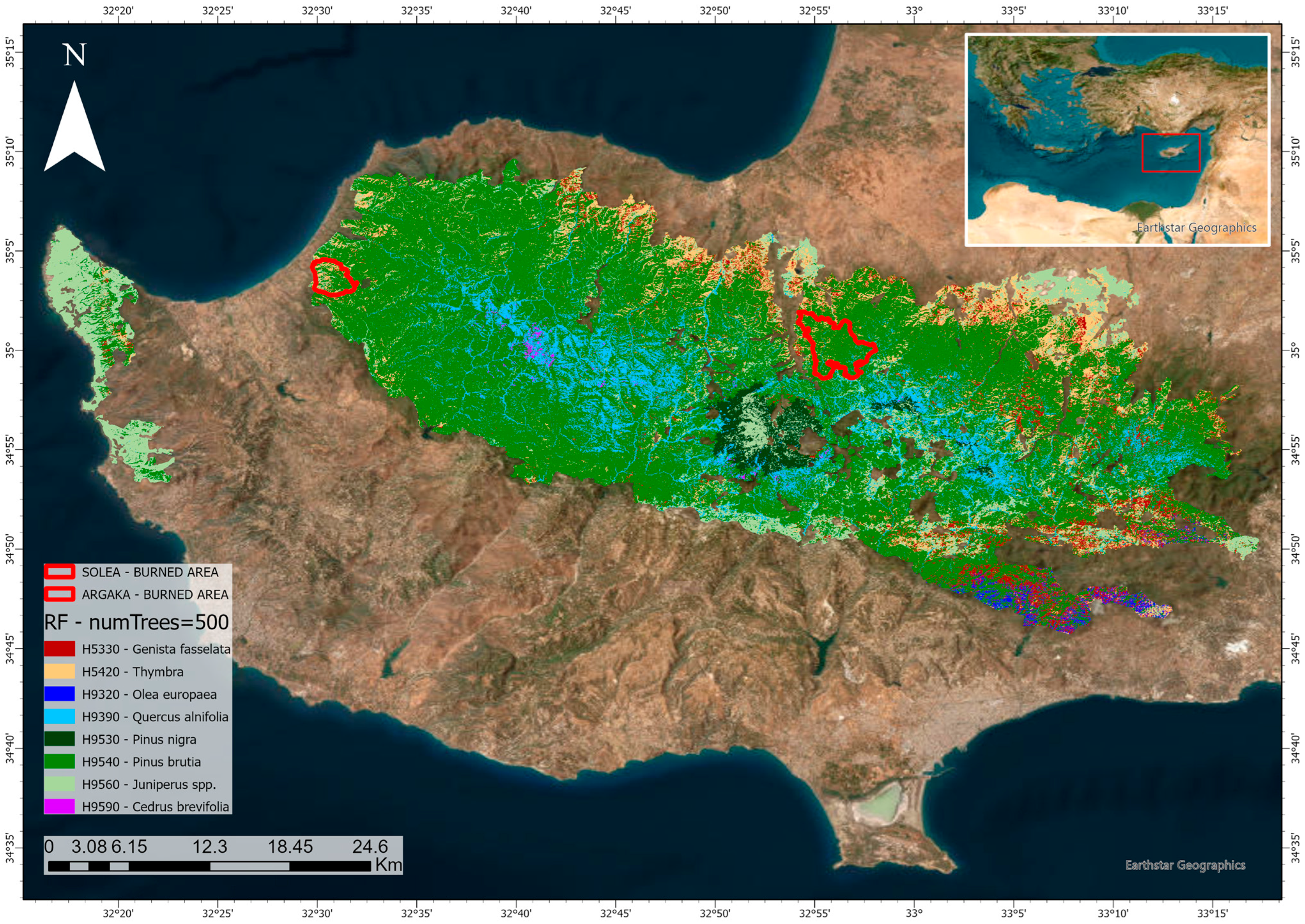
3.4. Spatial Distribution of Forest Habitats in the Study Area

As shown in Figure 7, the habitats are distributed as follows in the study area: most of the area consisted of H9540 (1050.84 km2, 64%) followed by H9560 (179.81 km2, 11%). Furthermore, H9390 and H5420 exhibit similar distributions covering 7.85% and 7.51%, respectively. H5330 covers 6% of the area. Additionally, H9530, H9320, and H9590 have the smallest percentages in this study area, covering 2.30%, 0.65%, and 0.31% of the total area, respectively. Focusing on burned areas, in Arkaga, the fire ignition destroyed a total of 7.63 km2 where 4.43 km2 constituted H9540, and a small part is constituted by H5420 (1.57 km2), H9560 (1.1 km2), and a very small part is characterized by H5330 (0.52 km2). Regarding the burned area in the Solea area, the fire event destroyed a total of 18.96 km2 where the majority of the burned area is characterized by H9540 (16.62 km2), and the remaining areas are H5330, H6520, H9390, and H9560.

4. Discussion

In Mediterranean ecosystems, the adaptation of forests to fire is widespread. In burned areas, regeneration may occur through seed germination [140], resprouting from burned trees and stumps [141], or through the resprouting of burned shrubs or herbs [142]. However, there are forest ecosystems that have not developed natural mechanisms of adaptation and regeneration after fire events, such as black pine and species of the genus Juniperus. In these cases, restoration is achieved mainly through reforestation [143]. In this context, forest restoration plays a crucial role in recovering ecosystems that have been degraded or destroyed, such as after wildfire events, by aiming to restore their ecological integrity and resilience [6,7]. In the context of climate change, habitat mapping also plays a crucial role in supporting long-term forest resilience by informing adaptive habitat selection. Future environmental shifts may reduce the viability of currently dominant habitats, such as Pinus brutia, highlighting the need to prioritize habitats better suited to future climatic conditions to ensure ecosystem resilience and the continued provision of key services such as carbon sequestration and biodiversity conservation [144].
Accurately mapping the distribution of forest habitats, as undertaken in this study, provides essential baseline information for identifying current habitat distributions and guiding future restoration and reforestation planning. The primary objective of this study was to map the dominant forest habitats in forest areas of particular interest in Cyprus. The retrieval of this information plays a crucial role, especially in restoration actions in areas affected by fires, such as Solea and Argaka, areas where reforestation actions have been implemented by the Department of Forests in Cyprus.
This study examines the performance of three supervised pixel-based nonparametric algorithms, RF, SVM, and CART, using the dataset proposed by Prodromou et al. [88] which includes Sentinel-2 imagery (spectral bands and vegetation indices) and topographical features (elevation, aspect, and slope) processed through GEE. Additionally, as a second scenario, a dataset that is based on Dataset 1 but enhanced by the inclusion of additional spectral indices derived from Sentinel-1 and Sentinel-2 imagery and tree density data was utilized to improve habitats identification for targeted reforestation actions.
A total of eight classes were classified; however, the classification output analyses provide particular emphasis on habitat H9540, which is the dominant tree species in Cyprus, where its formation is distributed across 65% of the Cyprus forests [145].
The results derived from the proposed methodology indicate that SVM and RF outperformed CART, which is also confirmed by other studies [35,68,130,146,147]. The implementation of machine learning optimization through the GEE across extensive areas poses specific challenges, particularly with respect to computational time. Nevertheless, this paper also demonstrates the capability of the cloud-based free platform for conducting forest habitat distribution.
Although SVM presented higher accuracy based on OA and kappa statistics, RF appeared to provide greater stability across most habitats, especially for H9530 and H9540, which are the primary foci of this study. These findings align with those of previous research [146] and reinforce the reliability of RF in heterogeneous environments. Specifically, based on hyperparameter tuning, RF achieved the highest accuracy with the critical hyperparameter “numTrees” = 500 while the remaining parameters were set to their default values, thus achieving the maintenance of the balance between accuracy, generalization, and overfitting prevention. According to studies [32,148], the RF algorithm improves classification accuracy by generating an ensemble of multiple decision trees, thereby reducing model variance. Although SVM identified habitats with high accuracy using optimized (high) cost and gamma values, the trend for overfitting made it less suitable for operational mapping in this context. Thus, RF was selected as the preferred model for further applications, given its proven robustness [36,147,149].
Moreover, considering that each vegetation type varies significantly in aspects like moisture levels, seasonality, and plant structure, which can affect the classification process, another aspect that plays a crucial role despite the selection of the classification method [150,151] is the specific characteristics of the study area. This is particularly important because the variability in spectral responses within the same ecosystem and the similarity in spectral signatures across different ecosystem types can further complicate the classification tasks [152]. For this purpose, the comparison between the two datasets showed that the integration of Sentinel-1 and Sentinel-2 data, along with derived spectral indices as well as topographic features or other parameters such as tree density, can enhance the performance of the model, a finding also supported by other studies [88,147]. This finding is confirmed by the feature importance analysis, where the elevation was the most influential variable, with slope and aspect also ranking highly. Among the Sentinel-2 data, B9 and vegetation indices (GLI, NDMI, and NBRI) contributed significantly. However, NDVI had a lower impact despite its wide use and this finding also agrees with the findings of [153]. Also, the addition of Sentinel-1 bands, especially the VH polarization as well as the TD variable in Dataset 2, provides valuable insights into canopy structure.
It is worth noting that in both datasets, the performance of the models with the optimal hyperparameters was within acceptable limits; however, when considering the performance for each habitat based on F1-score evaluation, Dataset 2 consistently outperformed Dataset 1. This confirms that incorporating additional structural and spectral variables improves habitat discrimination.
Overall, this methodology not only achieves the accurate identification of the dominant habitats in forest areas but also enables temporal habitat mapping as the model can be applied across different time periods. This capability provides timely and valuable insights into habitat distribution, which is particularly important for the planning of restoration strategies in burned areas and other degraded forest environments.

Limitations of the Study and Future Work

Despite the promising results, several limitations should be acknowledged. In cases where small-scale heterogeneity exists, especially in mixed forest landscapes, the use of Sentinel-2 images with a spatial resolution of 10–20 m is limited. Furthermore, Sentinel-2 data, being optical data, are affected by the presence of cloud occurrence that introduces biases, particularly in periods with higher cloud cover, such as during the winter months. Regarding the use of the GEE platform, the computational requirements associated with large-scale processing, although manageable in this study, may pose challenges for operational deployment over even larger areas or for higher resolution images. Finally, while the models achieved satisfactory accuracy, the generalizability of the classification approach to different Mediterranean regions with diverse ecological characteristics remains to be validated in future studies. Moreover, although this study focused on pixel-based classification methods due to their scalability and compatibility with GEE, we acknowledge that object-based image analysis (OBIA) and image segmentation algorithms (e.g., Watershed, Mean Shift, or DBSCAN) could offer enhanced delineation of habitat boundaries, particularly in heterogeneous landscapes or with higher resolution data. These approaches will be considered in future investigations, especially when applying the methodology outside the GEE environment or with finer-resolution imagery.
In addition, future work will also investigate the application of deep learning approaches such as Convolutional Neural Networks (CNNs) and Multilayer Perceptrons (MLPs) to enhance the classification of forest habitats further. Deep learning models offer significant potential for improving classification accuracy, particularly in complex and heterogeneous Mediterranean environments. Moreover, future efforts will focus on developing a comprehensive post-fire management tool for Mediterranean forest ecosystems, leveraging satellite data to support restoration strategies both during the selection of suitable reforestation habitats and in long-term monitoring to assess the effectiveness of restoration actions.

5. Conclusions

This study successfully developed an optimized remote sensing framework to address the critical need for precise and scalable habitat mapping in Mediterranean forests. By applying supervised non-parametric classification models in GEE, the dominant forest habitats in Cyprus were mapped with high ecological significance. We have demonstrated effective solutions to the challenges of distinguishing spectrally similar conifer habitats and optimizing multi-source data fusion that were identified as key limitations in current monitoring approaches. Also, the study’s findings support global environmental strategies, such as the European Green Deal, the UN’s Decade on Ecosystem Restoration, and the Bonn Challenge, emphasizing the importance of forest conservation in mitigating climate change and enhancing greenhouse gas absorption.
Specifically, RF, SVM, and CART were evaluated, showing that SVM with an overall accuracy of 84.67% and RF at 82.24% outperformed CART which produced a lower accuracy of 77%. SVM achieves a slightly higher accuracy but shows greater sensitivity to hyperparameter tuning. Based on our analysis, which was conducted for the selection of the optimal classifier, RF was selected for habitat mapping due to its robustness and stability across different habitat types.
Moreover, this study examines the integration of Sentinel-1 and Sentinel-2, spectral indices, topographic features, and tree density. The study highlights the added value of integrating multisource remote sensing data. The findings show that the two datasets that were tested achieved similar and acceptable results, but Dataset 2 demonstrated improved performance across most hyperparameters. Specifically, high F1-scores were achieved for habitats such as H9540, reaching 89–90%, and H95300 and H9560, with scores of 87–88%, while lower classification accuracies were observed for more spectrally similar or less represented habitats such as H5330, H5420, and H9320 with F1-scores ranging from 20.31% to 53.78%.
Furthermore, based on the proposed methodology, the results show that the study area is mainly covered by Pinus brutia (H9540), covering 1050.84 km2, confirming that it is Cyprus’s primary and most important habitat. Given its extensive distribution, H9540 is also the most commonly used habitat for reforestation actions, so understanding its spatial distribution and temporal dynamics over the years is crucial for effective conservation planning, post-fire restoration, and sustainable forest management. This study supports post-fire restoration actions by aiding habitat selection for reforestation actions and enabling temporal habitat monitoring.
Our future work will focus on developing a post-fire management tool for Mediterranean ecosystems using satellite data to support restoration planning and long-term ecosystem assessment.

Author Contributions

Conceptualization, M.P. and I.G.; methodology, M.P.; software, M.P.; validation, M.P., M.T., and C.M.; formal analysis, M.P.; investigation, M.P.; resources, M.P.; data curation, M.P.; writing—original draft preparation, M.P., I.G., M.T., C.M., C.D., and D.H.; writing—review and editing, M.P., I.G., C.M., M.T., C.D., and D.H.; visualization, M.P.; supervision, D.H. and I.G. All authors have read and agreed to the published version of the manuscript.

Funding

This work was funded through the EXCELSIOR Teaming project (Grant Agreement No. 857510, www.excelsior2020.eu, accessed on 11 March 2025) that has received funding from the European Union’s Horizon 2020 research and innovation program and from the Government of the Republic of Cyprus through the Directorate General for the European Programmes, Coordination and Development.

Institutional Review Board Statement

Not applicable.

Informed Consent Statement

Not applicable.

Data Availability Statement

Data are contained within the article.

Acknowledgments

The authors acknowledge the “‘EXCELSIOR’”: ERATOSTHENES: Excellence Research Centre for Earth Surveillance and Space-Based Monitoring of the Environment H2020 Widespread Teaming project (www.excelsior2020.eu, accessed on 11 March 2025). The “‘EXCELSIOR”’ project has received funding from the European Union’s Horizon 2020 research and innovation program under Grant Agreement No. 857510 from the Government of the Republic of Cyprus through the Directorate General for the European Programmes, Coordination and Development and the Cyprus University of Technology.

Conflicts of Interest

The authors declare no conflicts of interest.

Appendix A

Table A1. Hyperparameter configurations and their corresponding codes across the different classifiers.
HyperparametersHyperparameters Code
numTrees = 50RF_1
numTrees = 100RF_2
numTrees = 500RF_3
maxNodes = 10, minLeafPopulation = 1, numTrees = 50RF_4
maxNodes = 10, minLeafPopulation = 1, numTrees = 100RF_5
maxNodes = 10, minLeafPopulation = 1, numTrees = 500RF_6
maxNodes = 30, minLeafPopulation = 1, numTrees = 50RF_7
maxNodes = 30, minLeafPopulation = 1, numTrees = 100RF_8
maxNodes = 30, minLeafPopulation = 1, numTrees = 500RF_9
maxNodes = 100, minLeafPopulation = 1, numTrees = 50RF_10
maxNodes = 100, minLeafPopulation = 1, numTrees = 100RF_11
maxNodes = 100, minLeafPopulation = 1, numTrees = 500RF_12
maxNodes = 10, minLeafPopulation = 10, numTrees = 50RF_13
maxNodes = 10, minLeafPopulation = 10, numTrees = 100RF_14
maxNodes = 10, minLeafPopulation = 10, numTrees = 500RF_15
maxNodes = 30, minLeafPopulation = 10, numTrees = 50RF_16
maxNodes = 30, minLeafPopulation = 10, numTrees = 100RF_17
maxNodes = 30, minLeafPopulation = 10, numTrees = 500RF_18
maxNodes = 100, minLeafPopulation = 10, numTrees = 50RF_19
maxNodes = 100, minLeafPopulation = 10, numTrees = 100RF_20
maxNodes = 100, minLeafPopulation = 10, numTrees = 500RF_21
maxNodes = 10, minLeafPopulation = 50, numTrees = 50RF_22
maxNodes = 10, minLeafPopulation = 50, numTrees = 100RF_23
maxNodes = 10, minLeafPopulation = 50, numTrees = 500RF_24
maxNodes = 30, minLeafPopulation = 50, numTrees = 50RF_25
maxNodes = 30, minLeafPopulation = 50, numTrees = 100RF_26
maxNodes = 30, minLeafPopulation = 50, numTrees = 500RF_26
maxNodes = 100, minLeafPopulation = 50, numTrees = 50RF_27
maxNodes = 100, minLeafPopulation = 50, numTrees = 100RF_28
maxNodes = 100, minLeafPopulation = 50, numTrees = 500RF_29
cost = 1, kernel = RBF, gamma = 0.01SVM_1
cost = 10, kernel = RBF, gamma = 0.01SVM_2
cost = 50, kernel = RBF, gamma = 0.01SVM_3
cost = 100, kernel = RBF, gamma = 0.01SVM_4
cost = 1, kernel = RBF, gamma = 0.04SVM_5
cost = 10, kernel = RBF, gamma = 0.04SVM_6
cost = 50, kernel = RBF, gamma = 0.04SVM_7
cost = 100, kernel = RBF, gamma = 0.04SVM_8
cost = 1, kernel = RBF, gamma = 0.1SVM_9
cost = 10, kernel = RBF, gamma = 0.1SVM_10
cost = 50, kernel = RBF, gamma = 0.1SVM_11
cost = 100, kernel = RBF, gamma = 0.1SVM_12
cost = 1, kernel = RBF, gamma = 0.5SVM_13
cost = 10, kernel = RBF, gamma = 0.5SVM_14
cost = 50, kernel = RBF, gamma = 0.5SVM_15
cost = 100, kernel = RBF, gamma = 0.5SVM_16
cost = 1, kernel = RBF, gamma = 1SVM_17
cost = 10, kernel = RBF, gamma = 1SVM_18
cost = 50, kernel = RBF, gamma = 1SVM_19
cost = 100, kernel = RBF, gamma = 1SVM_20
maxNodes = 10, minLeafPopulation = 1CART_1
maxNodes = 10, minLeafPopulation = 10CART_2
maxNodes = 10, minLeafPopulation = 50CART_3
maxNodes = 30, minLeafPopulation = 1CART_4
maxNodes = 30, minLeafPopulation = 10CART_5
maxNodes = 30, minLeafPopulation = 50CART_6
maxNodes = 50, minLeafPopulation = 1CART_7
maxNodes = 50, minLeafPopulation = 10CART_8
maxNodes = 50, minLeafPopulation = 50CART_9
maxNodes = 100, minLeafPopulation = 1CART_10
maxNodes = 100, minLeafPopulation = 10CART_11
maxNodes = 100, minLeafPopulation = 50CART_12
maxNodes = 500, minLeafPopulation = 1CART_13
maxNodes = 500, minLeafPopulation = 10CART_14
maxNodes = 500, minLeafPopulation = 50CART_15
minLeafPopulation = 1CART_16

Appendix B

Figure A1. Hyperparameter tuning in the 5-fold cross-validation based on the OA for Dataset 1. OA greater than 80% are marked (*).
Sustainability 17 06021 g0a1
Figure A2. Hyperparameter tuning in the 5-fold cross-validation based on the OA based on Dataset 2. OA greater than 80% are marked (*).
Sustainability 17 06021 g0a2
Figure A3. Variable importance in Random Forest (RF) across the different hyperparameters.
Sustainability 17 06021 g0a3

References

  1. Alayan, R.; Rotich, B.; Lakner, Z. A Comprehensive Framework for Forest Restoration after Forest Fires in Theory and Practice: A Systematic Review. Forests 2022, 13, 1354. [Google Scholar] [CrossRef]
  2. Pausas, J.G.; Vallejo, V.R. The Role of Fire in European Mediterranean Ecosystems. In Remote Sensing of Large Wildfires; Springer: Berlin/Heidelberg, Germany, 1999; pp. 3–16. [Google Scholar]
  3. van Lierop, P.; Lindquist, E.; Sathyapala, S.; Franceschini, G. Global Forest Area Disturbance from Fire, Insect Pests, Diseases and Severe Weather Events. For. Ecol. Manag. 2015, 352, 78–88. [Google Scholar] [CrossRef]
  4. Timbal, J.; Bonneau, M.; Landmann, G.; Trouvilliez, J.; Bouhot-Delduc, L. European Non Boreal Conifer Forests. In Ecosystems of the World (6): Coniferous Forests; Elsevier: Amsterdam, The Netherlands, 2005; pp. 131–162. [Google Scholar]
  5. Farjon, A.; Filer, D. An Atlas of the World’s Conifers: An Analysis of Their Distribution, Biogeography, Diversity and Conservation Status; Brill: Leiden, The Netherlands, 2013; ISBN 9004211810. [Google Scholar]
  6. Bonari, G.; Fernández-González, F.; Çoban, S.; Monteiro-Henriques, T.; Bergmeier, E.; Didukh, Y.P.; Xystrakis, F.; Angiolini, C.; Chytrý, K.; Acosta, A.T.R.; et al. Classification of the Mediterranean Lowland to Submontane Pine Forest Vegetation. Appl. Veg. Sci. 2021, 24, e12544. [Google Scholar] [CrossRef]
  7. Quézel, P.; Barbero, M. Aperçu Syntaxinomique Sur La Connaissance Actuelle de La Classe Des Quercetea Ilicis Au Maroc. Ecol. Mediterr. 1986, 12, 105–111. [Google Scholar] [CrossRef]
  8. Barbéro, M.; Loisel, R.; Quézel, P.; Richardson, D.M.; Romane, F. Ecology and Biogeography of Pinus; Cambridge University Press: Cambridge, UK, 1998. [Google Scholar]
  9. Delipetrou, P.; Makhzoumi, J.; Dimopoulos, P.; Georghiou, K. Cyprus. In Mediterranean Island Landscapes: Natural and Cultural Approaches; Springer Science & Business Media: Berlin, Germany, 2008; pp. 170–203. [Google Scholar]
  10. Kitikidou, K.; Petrou, P.; Milios, E. Dominant Height Growth and Site Index Curves for Calabrian Pine (Pinus brutia Ten.) in Central Cyprus. Renew. Sustain. Energy Rev. 2012, 16, 1323–1329. [Google Scholar] [CrossRef]
  11. Pantelas, V. The Forests of Brutia Pine in Cyprus. Options Mediterr. 1986, 86, 46. [Google Scholar]
  12. Petrou, P.; Milios, E. Investigation of the Factors Affecting Artificial Seed Sowing Success and Seedling Survival in Pinus brutia Natural Stands in Middle Elevations of Central Cyprus. Forests 2020, 11, 1349. [Google Scholar] [CrossRef]
  13. Fady, B.; Semerci, H.; Vendramin, G.G. EUFORGEN Technical Guidelines for Genetic Conservation and Use for Aleppo Pine (Pinus halepensis) and Brutia Pine (Pinus brutia); Bioversity International: Rome, Italy, 2003; ISBN 9290435712. [Google Scholar]
  14. Burylo, M.; Rey, F.; Bochet, E.; Dutoit, T. Plant Functional Traits and Species Ability for Sediment Retention during Concentrated Flow Erosion. Plant Soil 2012, 353, 135–144. [Google Scholar] [CrossRef]
  15. Torres, I.; Moreno, J.M.; Morales-Molino, C.; Arianoutsou, M. Ecosystem Services Provided by Pine Forests. In Pines and Their Mixed Forest Ecosystems in the Mediterranean Basin; Springer International Publishing: Cham, Switzerland, 2021; pp. 617–629. [Google Scholar]
  16. Crouzeilles, R.; Ferreira, M.S.; Chazdon, R.L.; Lindenmayer, D.B.; Sansevero, J.B.B.; Monteiro, L.; Iribarrem, A.; Latawiec, A.E.; Strassburg, B.B.N. Ecological Restoration Success Is Higher for Natural Regeneration than for Active Restoration in Tropical Forests. Sci. Adv. 2017, 3, e1701345. [Google Scholar] [CrossRef]
  17. Fassnacht, F.E.; Latifi, H.; Stereńczak, K.; Modzelewska, A.; Lefsky, M.; Waser, L.T.; Straub, C.; Ghosh, A. Review of Studies on Tree Species Classification from Remotely Sensed Data. Remote Sens. Environ. 2016, 186, 64–87. [Google Scholar] [CrossRef]
  18. Spurr, S.H. Aerial Photographs in Forestry; Ronald Press Co.: New York, NY, USA, 1948. [Google Scholar]
  19. Wan, H.; Tang, Y.; Jing, L.; Li, H.; Qiu, F.; Wu, W. Tree Species Classification of Forest Stands Using Multisource Remote Sensing Data. Remote Sens. 2021, 13, 144. [Google Scholar] [CrossRef]
  20. Zhang, D.; Qi, H.; Guo, X.; Sun, H.; Min, J.; Li, S.; Hou, L.; Lv, L. Integration of UAV Multispectral Remote Sensing and Random Forest for Full-Growth Stage Monitoring of Wheat Dynamics. Agriculture 2025, 15, 353. [Google Scholar] [CrossRef]
  21. Keskes, M.I.; Mohamed, A.H.; Borz, S.A.; Niţă, M.D. Improving National Forest Mapping in Romania Using Machine Learning and Sentinel-2 Multispectral Imagery. Remote Sens. 2025, 17, 715. [Google Scholar] [CrossRef]
  22. Kacic, P.; Kuenzer, C. Forest Biodiversity Monitoring Based on Remotely Sensed Spectral Diversity—A Review. Remote Sens. 2022, 14, 5363. [Google Scholar] [CrossRef]
  23. Kanja, K.; Zhang, C.; Atkinson, P.M. Evaluating Multi-Seasonal SAR and Optical Imagery for above-Ground Biomass Estimation Using the National Forest Inventory of Zambia. Int. J. Appl. Earth Obs. Geoinf. 2025, 139, 104494. [Google Scholar] [CrossRef]
  24. Lukman Alage, I.; Tan, Y.; Wasiu Akande, A.; Suprijanto, A. Advanced Characterization of Deforestation Frontiers in Nigeria Utilizing Deep Learning and Bayesian Approaches with Sentinel-1 SAR Imagery. Geocarto Int. 2025, 40, 2451164. [Google Scholar] [CrossRef]
  25. Agost, L.; Pascual, I.; Britos, H.A. Use of Argentine SAOCOM SAR Polarimetric L-Band Satellites for Classification of Arid and Semiarid Native Forests. Int. J. Remote Sens. 2025, 46, 2568–2586. [Google Scholar] [CrossRef]
  26. Dubayah, R.O.; Drake, J.B. Lidar Remote Sensing for Forestry. J. For. 2000, 98, 44–46. [Google Scholar] [CrossRef]
  27. Dubayah, R.; Blair, J.B.; Goetz, S.; Fatoyinbo, L.; Hansen, M.; Healey, S.; Hofton, M.; Hurtt, G.; Kellner, J.; Luthcke, S.; et al. The Global Ecosystem Dynamics Investigation: High-Resolution Laser Ranging of the Earth’s Forests and Topography. Sci. Remote Sens. 2020, 1, 100002. [Google Scholar] [CrossRef]
  28. Prodromou, M.; Theocharidis, C.; Fotiou, K.; Argyriou, A.; Polydorou, T.; Hadjimitsis, D.; Tzouvaras, M. Fusion of Sentinel-1 and Sentinel-2 Satellite Imagery to Rapidly Detect Landslides through Google Earth Engine 2023. In EGU General Assembly Conference Abstracts; Copernicus Publications: Göttingen, Germany, 2023. [Google Scholar]
  29. Duan, R.; Huang, C.; Dou, P.; Hou, J.; Zhang, Y.; Gu, J. Fine-Scale Forest Classification with Multi-Temporal Sentinel-1/2 Imagery Using a Temporal Convolutional Neural Network. Int. J. Digit. Earth 2025, 18, 2457953. [Google Scholar] [CrossRef]
  30. Vittucci, C.; Cordari, F.; Guerriero, L.; Di Sanzo, P. Design and Evaluation of a Cloud-Oriented Procedure Based on SAR and Multispectral Data to Detect Burnt Areas. Earth Sci. Inform. 2025, 18, 322. [Google Scholar] [CrossRef]
  31. Adugna, T.; Xu, W.; Fan, J. Comparison of Random Forest and Support Vector Machine Classifiers for Regional Land Cover Mapping Using Coarse Resolution FY-3C Images. Remote Sens. 2022, 14, 574. [Google Scholar] [CrossRef]
  32. Ewunetu, A.; Abebe, G. Integrating Google Earth Engine and Random Forest for Land Use and Land Cover Change Detection and Analysis in the Upper Tekeze Basin. Earth Sci. Inform. 2025, 18, 227. [Google Scholar] [CrossRef]
  33. Asif, M.; Kazmi, J.H.; Tariq, A.; Zhao, N.; Guluzade, R.; Soufan, W.; Almutairi, K.F.; Sabagh, A.E.; Aslam, M. Modelling of Land Use and Land Cover Changes and Prediction Using CA-Markov and Random Forest. Geocarto Int. 2023, 38, 2210532. [Google Scholar] [CrossRef]
  34. Tariq, A.; Jiango, Y.; Li, Q.; Gao, J.; Lu, L.; Soufan, W.; Almutairi, K.F.; Habib-ur-Rahman, M. Modelling, Mapping and Monitoring of Forest Cover Changes, Using Support Vector Machine, Kernel Logistic Regression and Naive Bayes Tree Models with Optical Remote Sensing Data. Heliyon 2023, 9, e13212. [Google Scholar] [CrossRef]
  35. Monteiro, L.; Almeida, B.; Duarte, B.; Cabral, P. Framing the Forest: A Comparative Analysis of Google Earth Engine Classifiers for Accurate Species Extraction. In International Conference on Geospatial Information Sciences; Springer Nature: Cham, Switzerland, 2024; pp. 159–171. [Google Scholar]
  36. Lin, C.; Zheng, J.; Hu, L.; Chen, L. Extraction of Mangrove Community of Kandelia Obovata in China Based on Google Earth Engine and Dense Sentinel-1/2 Time Series Data. Remote Sens. 2025, 17, 898. [Google Scholar] [CrossRef]
  37. Nguyen Thanh Le, V.; Apopei, B.; Alameh, K. Effective Plant Discrimination Based on the Combination of Local Binary Pattern Operators and Multiclass Support Vector Machine Methods. Inf. Process. Agric. 2019, 6, 116–131. [Google Scholar] [CrossRef]
  38. Kour, V.P.; Arora, S. Particle Swarm Optimization Based Support Vector Machine (P-SVM) for the Segmentation and Classification of Plants. IEEE Access 2019, 7, 29374–29385. [Google Scholar] [CrossRef]
  39. Chandra, M.A.; Bedi, S.S. Survey on SVM and Their Application in Image Classification. Int. J. Inf. Technol. 2021, 13, 1–11. [Google Scholar] [CrossRef]
  40. Akbarzadeh, S.; Paap, A.; Ahderom, S.; Apopei, B.; Alameh, K. Plant Discrimination by Support Vector Machine Classifier Based on Spectral Reflectance. Comput. Electron. Agric. 2018, 148, 250–258. [Google Scholar] [CrossRef]
  41. Ma, M.; Liu, J.; Liu, M.; Zeng, J.; Li, Y. Tree Species Classification Based on Sentinel-2 Imagery and Random Forest Classifier in the Eastern Regions of the Qilian Mountains. Forests 2021, 12, 1736. [Google Scholar] [CrossRef]
  42. Immitzer, M.; Atzberger, C.; Koukal, T. Tree Species Classification with Random Forest Using Very High Spatial Resolution 8-Band WorldView-2 Satellite Data. Remote Sens. 2012, 4, 2661–2693. [Google Scholar] [CrossRef]
  43. Chaudhary, A.; Kolhe, S.; Kamal, R. An Improved Random Forest Classifier for Multi-Class Classification. Inf. Process. Agric. 2016, 3, 215–222. [Google Scholar] [CrossRef]
  44. Belgiu, M.; Drăguţ, L. Random Forest in Remote Sensing: A Review of Applications and Future Directions. ISPRS J. Photogramm. Remote Sens. 2016, 114, 24–31. [Google Scholar] [CrossRef]
  45. Aji, M.A.P.; Kamal, M.; Farda, N.M. Mangrove Species Mapping through Phenological Analysis Using Random Forest Algorithm on Google Earth Engine. Remote Sens. Appl. 2023, 30, 100978. [Google Scholar] [CrossRef]
  46. Magidi, J.; Nhamo, L.; Mpandeli, S.; Mabhaudhi, T. Application of the Random Forest Classifier to Map Irrigated Areas Using Google Earth Engine. Remote Sens. 2021, 13, 876. [Google Scholar] [CrossRef]
  47. Cengiz, A.; Budak, M.; Yağmur, N.; Balçik, F. Comparison between Random Forest and Support Vector Machine Algorithms for LULC Classification. Int. J. Eng. Geosci. 2023, 8, 1–10. [Google Scholar]
  48. Zagajewski, B.; Kluczek, M.; Raczko, E.; Njegovec, A.; Dabija, A.; Kycko, M. Comparison of Random Forest, Support Vector Machines, and Neural Networks for Post-Disaster Forest Species Mapping of the Krkonoše/Karkonosze Transboundary Biosphere Reserve. Remote Sens. 2021, 13, 2581. [Google Scholar] [CrossRef]
  49. Raczko, E.; Zagajewski, B. Comparison of Support Vector Machine, Random Forest and Neural Network Classifiers for Tree Species Classification on Airborne Hyperspectral APEX Images. Eur. J. Remote Sens. 2017, 50, 144–154. [Google Scholar] [CrossRef]
  50. Abdel-Rahman, E.M.; Mutanga, O.; Adam, E.; Ismail, R. Detecting Sirex Noctilio Grey-Attacked and Lightning-Struck Pine Trees Using Airborne Hyperspectral Data, Random Forest and Support Vector Machines Classifiers. ISPRS J. Photogramm. Remote Sens. 2014, 88, 48–59. [Google Scholar] [CrossRef]
  51. Rodriguez-Galiano, V.F.; Chica-Rivas, M. Evaluation of Different Machine Learning Methods for Land Cover Mapping of a Mediterranean Area Using Multi-Seasonal Landsat Images and Digital Terrain Models. Int. J. Digit. Earth 2014, 7, 492–509. [Google Scholar] [CrossRef]
  52. van Beijma, S.; Comber, A.; Lamb, A. Random Forest Classification of Salt Marsh Vegetation Habitats Using Quad-Polarimetric Airborne SAR, Elevation and Optical RS Data. Remote Sens. Environ. 2014, 149, 118–129. [Google Scholar] [CrossRef]
  53. Knauer, U.; von Rekowski, C.S.; Stecklina, M.; Krokotsch, T.; Pham Minh, T.; Hauffe, V.; Kilias, D.; Ehrhardt, I.; Sagischewski, H.; Chmara, S. Tree Species Classification Based on Hybrid Ensembles of a Convolutional Neural Network (CNN) and Random Forest Classifiers. Remote Sens. 2019, 11, 2788. [Google Scholar] [CrossRef]
  54. Zhang, B.; Zhao, L.; Zhang, X. Three-Dimensional Convolutional Neural Network Model for Tree Species Classification Using Airborne Hyperspectral Images. Remote Sens. Environ. 2020, 247, 111938. [Google Scholar] [CrossRef]
  55. El Sakka, M.; Ivanovici, M.; Chaari, L.; Mothe, J. A Review of CNN Applications in Smart Agriculture Using Multimodal Data. Sensors 2025, 25, 472. [Google Scholar] [CrossRef]
  56. Pongiannan, R.K.; Das, S.; Purbia, R.P.; Brindha, R.; Jame, S.L.; Shiju Kumar, P.S. Application of CNN Based Deep Learning Algorithm for Herbal Plant Leaf Detection. In Proceedings of the 2025 International Conference on Multi-Agent Systems for Collaborative Intelligence (ICMSCI), Erode, India, 20–22 January 2025; IEEE: Piscataway, NJ, USA; pp. 1817–1821. [Google Scholar]
  57. Xi, Y.; Ren, C.; Tian, Q.; Ren, Y.; Dong, X.; Zhang, Z. Exploitation of Time Series Sentinel-2 Data and Different Machine Learning Algorithms for Detailed Tree Species Classification. IEEE J. Sel. Top. Appl. Earth Obs. Remote Sens. 2021, 14, 7589–7603. [Google Scholar] [CrossRef]
  58. Reuß, F.; Greimeister-Pfeil, I.; Vreugdenhil, M.; Wagner, W. Comparison of Long Short-Term Memory Networks and Random Forest for Sentinel-1 Time Series Based Large Scale Crop Classification. Remote Sens. 2021, 13, 5000. [Google Scholar] [CrossRef]
  59. Kanagaraj, K.; Kulandaivel, M.; Shajin, F.H.; Prabhakaran, S. Leveraging Constitutive Artificial Neural Networks for Plant Leaf Disease Detection. Int. J. Ad Hoc Ubiquitous Comput. 2025, 48, 117–129. [Google Scholar] [CrossRef]
  60. He, T.; Zhou, H.; Xu, C.; Hu, J.; Xue, X.; Xu, L.; Lou, X.; Zeng, K.; Wang, Q. Deep Learning in Forest Tree Species Classification Using Sentinel-2 on Google Earth Engine: A Case Study of Qingyuan County. Sustainability 2023, 15, 2741. [Google Scholar] [CrossRef]
  61. McCormick, R.; Thenkabail, P.S.; Aneece, I.; Teluguntla, P.; Oliphant, A.J.; Foley, D. Artificial Neural Network Multi-Layer Perceptron Models to Classify California’s Crops Using Harmonized Landsat Sentinel (HLS) Data. Photogramm. Eng. Remote Sens. 2025, 91, 91–100. [Google Scholar] [CrossRef]
  62. Basri, B.; Karim, H.A.; Assidiq, M.; Arafah, M.; Rahmadani, F. Multilayer Perceptron Model with Feature Extraction for Potassium Deficiency Identification of Cocoa Plants. JOIV Int. J. Inform. Vis. 2025, 9, 324. [Google Scholar] [CrossRef]
  63. Amin, A.; Kamilaris, A. A Weakly Supervised Multimodal Deep Learning Approach for Large-Scale Tree Classification: A Case Study in Cyprus. Remote Sens. 2024, 16, 4611. [Google Scholar] [CrossRef]
  64. Masolele, R.N.; Sy, V.D.; Herold, M.; Marcos, D.; Verbesselt, J.; Gieseke, F.; Mullissa, A.G.; Martius, C. Remote Sensing of Environment Spatial and Temporal Deep Learning Methods for Deriving Land-Use Following Deforestation: A Pan-Tropical Case Study Using Landsat Time Series. Remote Sens. Environ. 2021, 264, 112600. [Google Scholar] [CrossRef]
  65. Mutanga, O.; Kumar, L. Google Earth Engine Applications. Remote Sens. 2019, 11, 591. [Google Scholar] [CrossRef]
  66. Papachristoforou, A.; Prodromou, M.; Hadjimitsis, D.; Christoforou, M. Detecting and Distinguishing between Apicultural Plants Using UAV Multispectral Imaging. PeerJ 2023, 11, e15065. [Google Scholar] [CrossRef]
  67. Kaplan, G. Broad-Leaved and Coniferous Forest Classification in Google Earth Engine Using Sentinel Imagery. Environ. Sci. Proc. 2021, 3, 64. [Google Scholar]
  68. Praticò, S.; Solano, F.; Di Fazio, S.; Modica, G. Machine Learning Classification of Mediterranean Forest Habitats in Google Earth Engine Based on Seasonal Sentinel-2 Time-Series and Input Image Composition Optimisation. Remote Sens. 2021, 13, 586. [Google Scholar] [CrossRef]
  69. Jahromi, M.N.; Jahromi, M.N.; Zolghadr-Asli, B.; Pourghasemi, H.R.; Alavipanah, S.K. Google Earth Engine and Its Application in Forest Sciences. In Spatial Modeling in Forest Resources Management: Rural Livelihood and Sustainable Development; Springer Nature: Cham, Switzerland, 2021; pp. 629–649. [Google Scholar]
  70. Bilotta, G.; Meduri, G.M.; Genovese, E.; Bibbò, L.; Barrile, V. Safeguarding the Aspromonte Forests: Random Forests and Markov Chains as Forecasting Models for Predicting Land Transformations. Forests 2025, 16, 290. [Google Scholar] [CrossRef]
  71. El Kharki, A.; Mechbouh, J.; Wahbi, M.; Alaoui, O.Y.; Boulaassal, H.; Maatouk, M.; El Kharki, O. Optimizing SVM for Argan Tree Classification Using Sentinel-2 Data: A Case Study in the Sous-Massa Region, Morocco. Rev. Teledetec. 2024, 65, 22060. [Google Scholar] [CrossRef]
  72. Prodromou, M.; Gitas, I.; Mettas, C.; Tzouvaras, M.; Themistocleous, K.; Konstantinidis, A.; Pamboris, A.; Hadjimitsis, D. Remote-Sensing-Based Prioritization of Post-Fire Restoration Actions in Mediterranean Ecosystems: A Case Study in Cyprus. Remote Sens. 2025, 17, 1269. [Google Scholar] [CrossRef]
  73. European Commission. EU Biodiversity Strategy for 2030; COM(2020) 380 final; European Commission: Brussels, Belgium, 2020; pp. 1–23. [Google Scholar]
  74. Soares, A.G. The European Green Deal. Rev. Jurid. Portucalense 2024, 35, 44–67. [Google Scholar] [CrossRef]
  75. Aragão, A.; Meertens, M.; Schoukens, H.; Decleer, K. The Negotiation Process of the EU Nature Restoration Law Proposal. Restor. Ecol. J. Soc. Ecol. Restor. 2024, 32, e14158. [Google Scholar]
  76. Martins, P.I.; Belém, L.B.C.; Szabo, J.K.; Libonati, R.; Garcia, L.C. Prioritising Areas for Wildfire Prevention and Post-Fire Restoration in the Brazilian Pantanal. Ecol. Eng. 2022, 176, 106517. [Google Scholar] [CrossRef]
  77. Tavşanoğlu, Ç.; Gürkan, B. Long-Term Post-Fire Dynamics of Co-Occurring Woody Species in Pinus brutia Forests: The Role of Regeneration Mode. Plant Ecol. 2014, 215, 355–365. [Google Scholar] [CrossRef]
  78. Bukała, M.; Zboińska, K.; Szadkowski, M. Troodos Ophiolite Mantle Section Exposed along Atalante Geo-Trail, Troodos Geopark, Cyprus. Geosci. Rec. 2016, 3, 1–6. [Google Scholar] [CrossRef]
  79. Fox, N.; Chamberlain, B.; Lindquist, M.; Van Berkel, D. Understanding Landscape Aesthetics Using a Novel Viewshed Assessment of Social Media Locations Within the Troodos UNESCO Global Geopark, Cyprus. Front. Environ. Sci. 2022, 10, 884115. [Google Scholar] [CrossRef]
  80. European Environment Agency. Natura 2000, Standard Data Form Site CY5000004. Available online: https://natura2000.eea.europa.eu/Natura2000/SDF.aspx?site=CY5000004 (accessed on 10 March 2025).
  81. European Environment Agency. Natura 2000, Standard Data Form Site CY2000006. Available online: https://natura2000.eea.europa.eu/Natura2000/SDF.aspx?site=CY2000006 (accessed on 9 March 2025).
  82. European Environment Agency. Natura 2000, Standard Data Form Site CY4000010. Available online: https://natura2000.eea.europa.eu/Natura2000/SDF.aspx?site=CY4000010 (accessed on 10 March 2025).
  83. European Environment Agency. Land Copernicus. Available online: https://land.copernicus.eu/en/products/high-resolution-layer-tree-cover-density/tree-cover-density-2015 (accessed on 9 March 2025).
  84. European Environment Agency. High Resolution Layer Tree Cover Density. Available online: https://land.copernicus.eu/en/products/high-resolution-layer-tree-cover-density (accessed on 6 April 2025).
  85. European Commission Council Directive 92/43/ECC. Off. J. Eur. Union. 1992, 94, 40–52.
  86. Balayn, A.; Soilis, P.; Lofi, C.; Yang, J.; Bozzon, A. What Do You Mean? Interpreting Image Classification with Crowdsourced Concept Extraction and Analysis. In Proceedings of the Web Conference 2021—Proceedings of the World Wide Web Conference, WWW 2021, Ljubljana, Slovenia, 19–23 April 2021; Volume 2, pp. 1937–1948. [Google Scholar] [CrossRef]
  87. Gautam, N.C. Aerial Photo-Interpretation Techniques for Classifying Urban Land Use. Photogramm. Eng. Remote Sens. 1976, 42, 815–822. [Google Scholar]
  88. Prodromou, M.; Theocharidis, C.; Gitas, I.Z.; Eliades, F.; Themistocleous, K.; Papasavvas, K.; Dimitrakopoulos, C.; Danezis, C.; Hadjimitsis, D. Forest Habitat Mapping in Natura2000 Regions in Cyprus Using Sentinel-1, Sentinel-2 and Topographical Features. Remote Sens. 2024, 16, 1373. [Google Scholar] [CrossRef]
  89. Wang, F.; Yang, S.; Yang, W.; Yang, X.; Jianli, D. Comparison of Machine Learning Algorithms for Soil Salinity Predictions in Three Dryland Oases Located in Xinjiang Uyghur Autonomous Region (XJUAR) of China. Eur. J. Remote Sens. 2019, 52, 256–276. [Google Scholar] [CrossRef]
  90. Wei, Y.; Shi, Z.; Biswas, A.; Yang, S.; Ding, J.; Wang, F. Updated Information on Soil Salinity in a Typical Oasis Agroecosystem and Desert-Oasis Ecotone: Case Study Conducted along the Tarim River, China. Sci. Total Environ. 2020, 716, 135387. [Google Scholar] [CrossRef]
  91. Xue, J.; Su, B. Significant Remote Sensing Vegetation Indices: A Review of Developments and Applications. J. Sens. 2017, 2017, 1353691. [Google Scholar] [CrossRef]
  92. Tran, T.V.; Reef, R.; Zhu, X. A Review of Spectral Indices for Mangrove Remote Sensing. Remote Sens. 2022, 14, 4868. [Google Scholar] [CrossRef]
  93. Younes Cárdenas, N.; Joyce, K.E.; Maier, S.W. Monitoring Mangrove Forests: Are We Taking Full Advantage of Technology? Int. J. Appl. Earth Obs. Geoinf. 2017, 63, 1–14. [Google Scholar] [CrossRef]
  94. Tucker, C.J. Red and Photographic Infrared Linear Combinations for Monitoring Vegetation. Remote Sens. Environ. 1979, 8, 127–150. [Google Scholar] [CrossRef]
  95. HUNTJR, E.; ROCK, B. Detection of Changes in Leaf Water Content Using Near- and Middle-Infrared Reflectances. Remote Sens. Environ. 1989, 30, 43–54. [Google Scholar] [CrossRef]
  96. Barnes, E.M.; Clarke, T.R.; Richards, S.E.; Colaizzi, P.D.; Haberland, J.; Kostrzewski, M.; Waller, P.; Choi, C.; Riley, E.; Thompson, T.; et al. Coincident Detection of Crop Water Stress, Nitrogen Status and Canopy Density Using Ground Based Multispectral Data. In Proceedings of the Fifth International Conference on Precision Agriculture, Bloomington, MN, USA, 16–19 July 2000. [Google Scholar]
  97. García, M.J.L.; Caselles, V. Mapping Burns and Natural Reforestation Using Thematic Mapper Data. Geocarto Int. 1991, 6, 31–37. [Google Scholar] [CrossRef]
  98. Key, C.H.; Benson, N.C. Landscape Assessment (LA) Sampling and Analysis Methods; General Technical Report RMRS-GTR; USDA Forest Service: Washington, DC, USA, 2006.
  99. Gerard, F.; Plummer, S.; Wadsworth, R.; Sanfeliu, A.F.; Iliffe, L.; Balzter, H.; Wyatt, B. Forest Fire Scar Detection in the Boreal Forest with Multitemporal Spot-Vegetation Data. IEEE Trans. Geosci. Remote Sens. 2003, 41, 2575–2585. [Google Scholar] [CrossRef]
  100. Alcaras, E.; Costantino, D.; Guastaferro, F.; Parente, C.; Pepe, M. Normalized Burn Ratio Plus (NBR+): A New Index for Sentinel-2 Imagery. Remote Sens. 2022, 14, 1727. [Google Scholar] [CrossRef]
  101. Chuvieco, E.; Martín, M.P.; Palacios, A. Assessment of Different Spectral Indices in the Red-near-Infrared Spectral Domain for Burned Land Discrimination. Int. J. Remote Sens. 2002, 23, 5103–5110. [Google Scholar] [CrossRef]
  102. Smith, A.M.S.; Drake, N.A.; Wooster, M.J.; Hudak, A.T.; Holden, Z.A.; Gibbons, C.J. Production of Landsat ETM+ Reference Imagery of Burned Areas within Southern African Savannahs: Comparison of Methods and Application to MODIS. Int. J. Remote Sens. 2007, 28, 2753–2775. [Google Scholar] [CrossRef]
  103. Trigg, S.; Flasse, S. An Evaluation of Different Bi-Spectral Spaces for Discriminating Burned Shrub-Savannah. Int. J. Remote Sens. 2001, 22, 2641–2647. [Google Scholar] [CrossRef]
  104. Jain, S.; Batra, K.U.; Mishra, P. Land Cover Classification by Decision Based Classifier Using Dual Polarimetric SAR Observables. In Proceedings of the 2022 IEEE 9th Uttar Pradesh Section International Conference on Electrical, Electronics and Computer Engineering (UPCON), Prayagraj, India, 2–4 December 2022; IEEE: Piscataway, NJ, USA, 2022; pp. 1–6. [Google Scholar]
  105. Kumar, D.; Rao, S.; Sharma, J.R. Radar Vegetation Index as an Alternative to NDVI for Monitoring of Soyabean and Cotton. In Proceedings of the XXXIII INCA International Congress (Indian Cartographer), Jodhpur, India, 19–21 September 2013; pp. 91–96. [Google Scholar]
  106. Xia, J.; Yokoya, N.; Pham, T.D. Probabilistic Mangrove Species Mapping with Multiple-Source Remote-Sensing Datasets Using Label Distribution Learning in Xuan Thuy National Park, Vietnam. Remote Sens. 2020, 12, 3834. [Google Scholar] [CrossRef]
  107. Mahdavi, S.; Salehi, B.; Amani, M.; Granger, J.; Brisco, B.; Huang, W. A Dynamic Classification Scheme for Mapping Spectrally Similar Classes: Application to Wetland Classification. Int. J. Appl. Earth Obs. Geoinf. 2019, 83, 101914. [Google Scholar] [CrossRef]
  108. Ghorbanian, A.; Zaghian, S.; Asiyabi, R.M.; Amani, M.; Mohammadzadeh, A.; Jamali, S. Mangrove Ecosystem Mapping Using Sentinel-1 and Sentinel-2 Satellite Images and Random Forest Algorithm in Google Earth Engine. Remote Sens. 2021, 13, 2565. [Google Scholar] [CrossRef]
  109. Kpienbaareh, D.; Sun, X.; Wang, J.; Luginaah, I.; Bezner Kerr, R.; Lupafya, E.; Dakishoni, L. Crop Type and Land Cover Mapping in Northern Malawi Using the Integration of Sentinel-1, Sentinel-2, and PlanetScope Satellite Data. Remote Sens. 2021, 13, 700. [Google Scholar] [CrossRef]
  110. De Luca, G.; Silva, J.M.N.; Di Fazio, S.; Modica, G. Integrated Use of Sentinel-1 and Sentinel-2 Data and Open-Source Machine Learning Algorithms for Land Cover Mapping in a Mediterranean Region. Eur. J. Remote Sens. 2022, 55, 52–70. [Google Scholar] [CrossRef]
  111. Yu, X.; Lu, D.; Jiang, X.; Li, G.; Chen, Y.; Li, D.; Chen, E. Examining the Roles of Spectral, Spatial, and Topographic Features in Improving Land-Cover and Forest Classifications in a Subtropical Region. Remote Sens. 2020, 12, 2907. [Google Scholar] [CrossRef]
  112. Lu, D.; Weng, Q. A Survey of Image Classification Methods and Techniques for Improving Classification Performance. Int. J. Remote Sens. 2007, 28, 823–870. [Google Scholar] [CrossRef]
  113. Gitelson, A.A.; Gritz, Y.; Merzlyak, M.N. Relationships between Leaf Chlorophyll Content and Spectral Reflectance and Algorithms for Non-Destructive Chlorophyll Assessment in Higher Plant Leaves. J. Plant Physiol. 2003, 160, 271–282. [Google Scholar] [CrossRef]
  114. Huete, A.; Didan, K.; Miura, T.; Rodriguez, E.P.; Gao, X.; Ferreira, L.G. Overview of the Radiometric and Biophysical Performance of the MODIS Vegetation Indices. Remote Sens. Environ. 2002, 83, 195–213. [Google Scholar] [CrossRef]
  115. Louhaichi, M.; Borman, M.M.; Johnson, D.E. Spatially Located Platform and Aerial Photography for Documentation of Grazing Impacts on Wheat. Geocarto Int. 2001, 16, 65–70. [Google Scholar] [CrossRef]
  116. Pen Uelas, J.; Filella, I.; Lloret, P.; Mun Oz, F.; Vilajeliu, M. Reflectance Assessment of Mite Effects on Apple Trees. Int. J. Remote Sens. 1995, 16, 2727–2733. [Google Scholar] [CrossRef]
  117. Kaufman, Y.J.; Tanre, D. Atmospherically Resistant Vegetation Index (ARVI) for EOS-MODIS. IEEE Trans. Geosci. Remote Sens. 1992, 30, 261–270. [Google Scholar] [CrossRef]
  118. Rikimaru, A.; Roy, P.; Miyatake, S. Tropical Forest Cover Density Mapping. Trop. Ecol. 2002, 43, 39–47. [Google Scholar]
  119. McFeeters, S.K. The Use of the Normalized Difference Water Index (NDWI) in the Delineation of Open Water Features. Int. J. Remote Sens. 1996, 17, 1425–1432. [Google Scholar] [CrossRef]
  120. Roy, P.S.; Sharma, K.P.; Jain, A. Stratification of Density in Dry Deciduous Forest Using Satellite Remote Sensing Digital Data—An Approach Based on Spectral Indices. J. Biosci. 1996, 21, 723–734. [Google Scholar] [CrossRef]
  121. Filipponi, F. BAIS2: Burned Area Index for Sentinel-2. Proceedings 2018, 2, 364. [Google Scholar] [CrossRef]
  122. Kim, Y.; Jackson, T.; Bindlish, R.; Lee, H. Sukyoung Hong Radar Vegetation Index for Estimating the Vegetation Water Content of Rice and Soybean. IEEE Geosci. Remote Sens. Lett. 2012, 9, 564–568. [Google Scholar] [CrossRef]
  123. Mitchard, E.T.A.; Saatchi, S.S.; White, L.J.T.; Abernethy, K.A.; Jeffery, K.J.; Lewis, S.L.; Collins, M.; Lefsky, M.A.; Leal, M.E.; Woodhouse, I.H.; et al. Mapping Tropical Forest Biomass with Radar and Spaceborne LiDAR in Lopé National Park, Gabon: Overcoming Problems of High Biomass and Persistent Cloud. Biogeosciences 2012, 9, 179–191. [Google Scholar] [CrossRef]
  124. Breiman, L.; Friedman, J.H.; Olshen, R.A.; Stone, C.J. Classification and Regression Trees; Routledge: Oxfordshire, UK, 1984; ISBN 9781315139470. [Google Scholar]
  125. Breiman, L. Random Forests. Mach. Learn. 2001, 45, 5–32. [Google Scholar] [CrossRef]
  126. Vorpahl, P.; Elsenbeer, H.; Märker, M.; Schröder, B. How Can Statistical Models Help to Determine Driving Factors of Landslides? Ecol. Modell. 2012, 239, 27–39. [Google Scholar] [CrossRef]
  127. Ließ, M.; Glaser, B.; Huwe, B. Uncertainty in the Spatial Prediction of Soil Texture. Geoderma 2012, 170, 70–79. [Google Scholar] [CrossRef]
  128. Cortes, C. Support-Vector Networks. Mach. Learn. 1995, 20, 273–297. [Google Scholar] [CrossRef]
  129. Bishop, C.M.; Nasrabadi, N.M. Pattern Recognition and Machine Learning; Springer: Berlin/Heidelberg, Germany, 2006; Volume 4. [Google Scholar]
  130. Hay Chung, L.C.; Xie, J.; Ren, C. Improved Machine-Learning Mapping of Local Climate Zones in Metropolitan Areas Using Composite Earth Observation Data in Google Earth Engine. Build. Environ. 2021, 199, 107879. [Google Scholar] [CrossRef]
  131. Ali, Y.; Awwad, E.; Al-Razgan, M.; Maarouf, A. Hyperparameter Search for Machine Learning Algorithms for Optimizing the Computational Complexity. Processes 2023, 11, 349. [Google Scholar] [CrossRef]
  132. Stromann, O.; Nascetti, A.; Yousif, O.; Ban, Y. Dimensionality Reduction and Feature Selection for Object-Based Land Cover Classification Based on Sentinel-1 and Sentinel-2 Time Series Using Google Earth Engine. Remote Sens. 2019, 12, 76. [Google Scholar] [CrossRef]
  133. Tselka, I.; Detsikas, S.E.; Petropoulos, G.P.; Demertzi, I.I. Google Earth Engine and Machine Learning Classifiers for Obtaining Burnt Area Cartography: A Case Study from a Mediterranean Setting. In Geoinformatics for Geosciences; Elsevier: Amsterdam, The Netherlands, 2023; pp. 131–148. [Google Scholar]
  134. Kazemi Garajeh, M. Monitoring the Spatio-Temporal Distribution of Soil Salinity Using Google Earth Engine for Detecting the Saline Areas Susceptible to Salt Storm Occurrence. Pollutants 2024, 4, 1–15. [Google Scholar] [CrossRef]
  135. Fathizad, H.; Ali Hakimzadeh Ardakani, M.; Sodaiezadeh, H.; Kerry, R.; Taghizadeh-Mehrjardi, R. Investigation of the Spatial and Temporal Variation of Soil Salinity Using Random Forests in the Central Desert of Iran. Geoderma 2020, 365, 114233. [Google Scholar] [CrossRef]
  136. Ramezan, C.A.; Warner, T.A.; Maxwell, A.E. Evaluation of Sampling and Cross-Validation Tuning Strategies for Regional-Scale Machine Learning Classification. Remote Sens. 2019, 11, 185. [Google Scholar] [CrossRef]
  137. Kuhn, M.; Johnson, K. Applied Predictive Modeling; Springer: New York, NY, USA, 2013; ISBN 978-1-4614-6848-6. [Google Scholar]
  138. James, G.; Witten, D.; Hastie, T.; Tibshirani, R.; Taylor, J. An Introduction to Statistical Learning; Springer Texts in Statistics; Springer International Publishing: Cham, Switzerland, 2023; ISBN 978-3-031-38746-3. [Google Scholar]
  139. Lee, J.S.H.; Wich, S.; Widayati, A.; Koh, L.P. Detecting Industrial Oil Palm Plantations on Landsat Images with Google Earth Engine. Remote Sens. Appl. 2016, 4, 219–224. [Google Scholar] [CrossRef]
  140. Pausas, J.G. Changes in Fire and Climate in the Eastern Iberian Peninsula (Mediterranean Basin). Clim. Chang. 2004, 63, 337–350. [Google Scholar] [CrossRef]
  141. Espelta, J.M.; Retana, J.; Habrouk, A. Resprouting Patterns after Fire and Response to Stool Cleaning of Two Coexisting Mediterranean Oaks with Contrasting Leaf Habits on Two Different Sites. For. Ecol. Manag. 2003, 179, 401–414. [Google Scholar] [CrossRef]
  142. Espelta, J.M.; Barbati, A.; Quevedo, L.; Tárrega, R.; Navascués, P.; Bonfil, C.; Peguero, G.; Fernández-Martínez, M.; Rodrigo, A. Post-Fire Management of Mediterranean Broadleaved Forests. In Post-Fire Management and Restoration of Southern European Forests; Springer: Dordrecht, The Netherlands, 2012; pp. 171–194. [Google Scholar]
  143. Turck, D.F.; Schwery, O.; Harmon, L.J.; Tank, D.C. Fire in the Tree: The Origin and Distribution of Fire–Adapted Traits within Conifers and Their Influence on Speciation Rates across the Conifer Phylogeny. Am. J. Bot. 2025, 112, e16454. [Google Scholar] [CrossRef]
  144. MacKenzie, W.H.; Mahony, C.R. An Ecological Approach to Climate Change-Informed Tree Species Selection for Reforestation. For. Ecol. Manag. 2021, 481, 118705. [Google Scholar] [CrossRef]
  145. Petrou, P.; Stampoulidis, A.; Pipinis, E.; Kitikidou, K.; Milios, E. Analysis of the Environments Where Natural Regeneration Is Established in the Absence of a Wildfire in the Open Pinus brutia Forests in the Middle Elevations of the Central Part of Cyprus. Forests 2024, 15, 1228. [Google Scholar] [CrossRef]
  146. Shaharum, N.S.N.; Shafri, H.Z.M.; Ghani, W.A.W.A.K.; Samsatli, S.; Al-Habshi, M.M.A.; Yusuf, B. Oil Palm Mapping over Peninsular Malaysia Using Google Earth Engine and Machine Learning Algorithms. Remote Sens. Appl. 2020, 17, 100287. [Google Scholar] [CrossRef]
  147. Pizarro, S.E.; Pricope, N.G.; Vargas-Machuca, D.; Huanca, O.; Ñaupari, J. Mapping Land Cover Types for Highland Andean Ecosystems in Peru Using Google Earth Engine. Remote Sens. 2022, 14, 1562. [Google Scholar] [CrossRef]
  148. Loukika, K.N.; Keesara, V.R.; Sridhar, V. Analysis of Land Use and Land Cover Using Machine Learning Algorithms on Google Earth Engine for Munneru River Basin, India. Sustainability 2021, 13, 13758. [Google Scholar] [CrossRef]
  149. Xie, B.; Cao, C.; Xu, M.; Duerler, R.S.; Yang, X.; Bashir, B.; Chen, Y.; Wang, K. Analysis of Regional Distribution of Tree Species Using Multi-Seasonal Sentinel-1&2 Imagery within Google Earth Engine. Forests 2021, 12, 565. [Google Scholar] [CrossRef]
  150. Mngadi, M.; Odindi, J.; Peerbhay, K.; Mutanga, O. Examining the Effectiveness of Sentinel-1 and 2 Imagery for Commercial Forest Species Mapping. Geocarto Int. 2021, 36, 1–12. [Google Scholar] [CrossRef]
  151. Sibanda, M.; Mutanga, O.; Rouget, M. Comparing the Spectral Settings of the New Generation Broad and Narrow Band Sensors in Estimating Biomass of Native Grasses Grown under Different Management Practices. GIsci Remote Sens. 2016, 53, 614–633. [Google Scholar] [CrossRef]
  152. Li, S.; Guo, P.; Sun, F.; Zhu, J.; Cao, X.; Dong, X.; Lu, Q. Mapping Dryland Ecosystems Using Google Earth Engine and Random Forest: A Case Study of an Ecologically Critical Area in Northern China. Land 2024, 13, 845. [Google Scholar] [CrossRef]
  153. Phan, T.N.; Kuch, V.; Lehnert, L.W. Land Cover Classification Using Google Earth Engine and Random Forest Classifier—The Role of Image Composition. Remote Sens. 2020, 12, 2411. [Google Scholar] [CrossRef]
Figure 1. Location map of the selected forest areas. Basemap source: Esri, Maxar, EarthstarGeographics, and the GIS user community.
Sustainability 17 06021 g001
Figure 2. Flow chart of the classification of the dominant forest habitats in Cyprus. Models achieving an overall accuracy (OA) of ≥80% were used for the development of the final habitat map; models with OA <80% (indicated in red) were excluded.
Sustainability 17 06021 g002
Figure 3. OA across different hyperparameters for Dataset 1.
Sustainability 17 06021 g003
Figure 4. OA across different hyperparameters for Dataset 2.
Sustainability 17 06021 g004
Figure 5. F1-score performance for each class through Datasets 1 and 2 per classifier.
Sustainability 17 06021 g005
Figure 6. Feature importance based on Dataset 2 for the RF_3 hyperparameter.
Sustainability 17 06021 g006
Figure 7. Distribution of the habitats across the study area.
Sustainability 17 06021 g007
Table 1. Habitat types were mapped according to the EU Habitat [85].
CodeHabitat
H9540Mediterranean pine forests with endemic Mesogean pines
H5420Sarcopoterium spinosum phrygana
H5330Thermo-Mediterranean and pre-desert scrub
H9320Olea and Ceratonia forests
H9390Scrub and low forest vegetation with Quercus alnifolia
H9560Endemic forests with Juniperus spp.
H9590Cedrus brevifolia forests (Cedrosetum brevifoliae)
H9530Mediterranean pine forests with endemic Mesogean pines
Table 2. Band combination protocols for experimental datasets.
DatasetsBand Combination
Dataset 1‘B2’, ‘B3’, ‘B4’, ‘B5’, ‘B6’, ‘B7’, ‘B8’, ‘B8A’, ’B11’, ’B12’, ’NDVI’, ’EVI’, ’SAVI’, ’NDMI’, ’NDRE1’, ’ELEVATION’, ’ASPECT’, ’SLOPE’
Dataset 2‘B2’, ‘B3’, ‘B4’, ‘B5’, ‘B6’, ‘B7’, ‘B8’, ‘B8A’, ‘B9’, ’B10’, ‘B11’, ‘B12’, ‘BSI’, ’ARVI’, ‘ASPECT’, ‘AVI’, ‘ELEVATION’, ‘EVI’, ‘GCI’, ‘GDVI’, ‘GLI’, ‘GNDVI’, ‘GOSAVI’, ‘GRVI’, ‘GSAVI’, ‘IPVI’, ‘NBRI’, ‘NDMI’, ‘NDRE1’, ‘NDVI’, ‘NDWI’, ‘RGR’, ‘SAVI’, ‘SIPI’, ‘SLOPE’, ‘TD’, ‘VH’, ‘VV’, ‘RVI’, ‘NRVI’
VV and VH = Polarization of S1, TD = Tree Density.
Disclaimer/Publisher’s Note: The statements, opinions and data contained in all publications are solely those of the individual author(s) and contributor(s) and not of MDPI and/or the editor(s). MDPI and/or the editor(s) disclaim responsibility for any injury to people or property resulting from any ideas, methods, instructions or products referred to in the content.

