Article

Assessment of Ecological Resilience and Identification of Influencing Factors in Jilin Province, China

School of Geographical Sciences and Tourism, Jilin Normal University, Siping 136000, China
*
Author to whom correspondence should be addressed.
Sustainability 2025, 17(13), 5994; https://doi.org/10.3390/su17135994
Submission received: 23 May 2025 / Revised: 21 June 2025 / Accepted: 27 June 2025 / Published: 30 June 2025

Abstract

Jilin Province is an important ecological security barrier and major grain-producing region in northeast China, playing a crucial role in ensuring ecological security and promoting regional sustainable development. This study examines ecological resilience from three dimensions: resistance, adaptability, and resilience. Based on multi-source data from 2000 to 2020, an ecological resilience indicator system was constructed. Spatial autocorrelation and OPGD models were employed to analyze temporal and spatial evolution and the driving mechanisms. The results indicate that ER exhibits an overall spatial pattern of “high in the east, low in the west, and under pressure in the central region.” The eastern mountainous areas demonstrate high and stable resilience, while the central plains and western ecologically fragile regions exhibit weaker resilience. In terms of resistance, the eastern mountainous regions are primarily forested, with high and sustained ESV, while the western sandy edge regions primarily have low ESV, making ecosystems susceptible to disturbance. In terms of adaptability, the large-scale farmland landscapes in the central regions exhibit strong disturbance resistance, while water resource adaptability in the western ecologically fragile regions has locally improved. However, adaptability in the eastern mountainous regions is relatively low due to development impacts. In terms of resilience, the eastern core regions possess stable recovery capabilities, while the central and western regions generally exhibit lower resistance with fluctuating changes. Between 2000 and 2020, the ecological resilience Moran’s I index slightly decreased from 0.558 to 0.554, with the spatial aggregation pattern remaining largely stable. Among the driving factors, DEM remains the most stable. The influence of NDVI has weakened, while temperature (TEM) and NPP-VIIRS have become more significant. Overall, factor interactions have grown stronger, as reflected by the q-value rising from 0.507 to 0.5605. This study provides theoretical support and decision-making references for enhancing regional ecological resilience, optimizing ecological spatial layout, and promoting sustainable ecosystem management.

Graphical Abstract

1. Introduction

A human–land relationship refers to the interaction between socio-economic activities and the natural geographic environment [1]. With rapid urbanization, human activity intensity has increased [2], altering human–land relationships and escalating pressure on ecosystems. If ecosystem service losses from environmental degradation exceed critical thresholds, irreversible ecological decline may occur, threatening regional ecological security [3]. Enhancing ecological resilience (ER) to recover from disturbances is now central to human–land systems [4]. Derived from Latin resilio (“to rebound”), ER initially described a physical system’s capacity to recover from shocks [5,6]. Holling [7] later applied it to ecology, defining it as an ecosystem’s ability to maintain structure and function after disturbance. Currently, unsustainable development models (marked by resource depletion, overconsumption, and pollution) have caused global ecological crises [8]. The COVID-19 pandemic further disrupted material production and resource supply [9], heightening regional ecological risks. Scholars broadly agree that regional resilience encompasses ecological, social, economic, institutional, and infrastructural dimensions [10,11]. As a key focus in resilience research [12,13], ER helps analyze human–land relationships and assess human impacts on environments [14,15,16]. Its goal is to maintain ecosystem stability amid environmental change. Given pressures like climate change, resource scarcity, and pollution, improving ER has become a critical task in ecology and environmental science.
For ecological resilience (ER) research, scholars have adopted different perspectives and methodologies. The research content is primarily categorized based on conceptual evolution [17,18], theoretical framework analysis [19], indicator system construction [20,21], resilience level measurement [22,23,24], and exploration of influencing mechanisms [25]. Among these, the construction of indicator systems is primarily based on statistical data or landscape ecology methods. Most studies using statistical data measure ER by calculating the weights of the ER indicator system. For example, Shi et al. (2022) constructed a 14-item indicator system based on three dimensions—ecological, social, and economic—to assess the ecological resilience level of the Beijing–Tianjin–Hebei urban agglomeration [26]. Some studies have also adopted the analytic hierarchy process [27]. Studies assessing ER from a landscape ecology perspective mostly construct multi-dimensional assessment models. For example, Liu et al. combined the coupling coordination model to systematically analyze the coupling and coordination relationship between new urbanization and ecological resilience in the Fen River Basin [28]. Feng et al. focused on Shenyang City, analyzing the patterns of urban resilience changes at different scales [29]; He et al. assessed the spatiotemporal evolution trends of urban resilience in the Chengdu–Deyang–Mianyang Economic Zone (2010–2020) [30]. There are also studies that assess ER based on characteristic dimensions (resistance, adaptability, and resilience). Jie et al. [31] took the Tao River Basin, an ecological transition zone, as a case study and refined the ecological safety pattern classification, emphasizing that different functional zones should adopt differentiated ecological governance strategies; Zhao et al. [32] studied the synergistic evolution and spatial convergence trends of economic development quality and ecological resilience in coastal urban agglomerations; Peng et al. [33] used Google Earth Engine and MODIS 500m data (spanning 2000–2020) to calculated the Remote Sensing Ecological Index (RSEI) and established a dual-indicator system for ecological environment quality and resilience. Regarding resilience measurement, most studies have constructed multi-dimensional assessment models, such as the structure–function model [34], which combines simulation of different disturbance scenarios to analyze the response and recovery capacity of Nanjing’s ecological network; the loss–benefit model [35] uses changes in ecosystem service capacity as the core indicator of ecological resilience, and employs GIS technology to assess the spatial distribution of ecological resilience in Tehran and identify vulnerable areas. Some studies have further developed other assessment models, such as the energy ecological footprint model [36], to assess the spatiotemporal changes in ecological pressure and ecological efficiency in China, exploring the impact of economic development on ecosystem resource consumption and carrying capacity. Based on the PSR framework, one study constructed an urban ecological resilience assessment indicator system to quantitatively assess the ecological resilience of the Pearl River Delta urban agglomeration [37]; and based on the PSR model, a rural ecological resilience measurement indicator system was constructed in another study, using Weiyuan County in Gansu Province as an example to assess its resilience level [38]. Additionally, the CRI model [39] and ND-GAIN model [40] were used to explore the dynamic evolution of regional ER. The enhancement of ecosystem service capacity is constrained and influenced by various factors, including economic, social, and natural factors. Economic factors are broad in scope, such as assessing the ecological resilience of 28 urban agglomerations in the middle reaches of the Yangtze River, analyzing the impact of economic development levels on ER [41]; resilience analysis of the Yangtze River Economic Belt also considered government green investment [42]. Social factors primarily encompass urbanization processes [43], with some studies also considering technological innovation capacity when analyzing the relationship between urbanization intensity and ecological resilience in the Beijing–Tianjin–Hebei integration region [44]. Natural factors focus on ecosystem service characteristics, such as the assessment of local ecological resilience in tourist destinations in the Dabie Mountains [45].
In ER assessments, the high dependence of landscape index calculations on a spatial scale makes selecting an appropriate spatial scale a fundamental prerequisite for ensuring the scientific rigor and reliability of the assessment. Landscape patterns are the result of various ecological processes at different scales and reflect landscape heterogeneity [46,47]. Fluctuations in landscape pattern indices and spatial autocorrelation parameters at different scales reflect the uncertainty introduced by the Modifiable Areal Unit Problem (MAUP). Therefore, a study should avoid arbitrarily setting the assessment unit scale and instead determine the optimal scale through empirical analysis [48]. Xie et al. [49] determined the optimal grid size to be 4.5 km by analyzing the response curves of landscape pattern indices and the variation characteristics of semivariogram parameters, arguing that inappropriate scales not only disrupt patch integrity but also obscure true spatial heterogeneity [50,51]. Therefore, it is necessary to determine the optimal scale before conducting an assessment to accurately and effectively reflect regional ER and existing issues. Jilin Province encompasses three major east–west ecological gradients: the forest ecosystem of Changbai Mountain, the agro-ecosystem of Songliao Plain, and the grassland ecosystem of Horqin. Given its unique geographic environment and rich natural resources, the province serves as a key research area for ecological resilience (ER). After identifying the optimal scale through semivariogram analysis, this study built an ER evaluation model based on resistance, adaptability, and resilience. Using land use data from 2000, 2010, and 2020, it analyzed ER patterns over time and applied the OPGD model to identify the key driving factors. Considering Jilin’s dual role as both a national food production hub and ecological barrier, this study’s findings can inform other regions facing trade-offs between agricultural intensification and ecosystem stability.

2. Materials and Methods

2.1. Study Area

Jilin Province (40°52′ N–46°18′ N, 121°38′ E–131°19′ E) is located in northeast China (Figure 1), covering a total area of 1.874 × 10⁷ hectares (approximately 1.95% of China’s land area). Administratively, it comprises 9 prefectures and 60 counties (cities/districts). As of 2023, Jilin Province’s urbanization rate was 64.72%, slightly below the national average (66.16%) but above the global average (57.25%); its regional gross domestic product was CNY 1.3531 trillion, far below the national total, indicating its position at the lower-middle level in the national development landscape, and it is currently in a phase of industrial structure transformation and steady urbanization progress. Climatically, the province experiences a temperate continental monsoon climate, with mean annual temperatures of 2–6 °C and annual precipitation of 400–600 mm, showing a transition from humid conditions in the southeast to semi-arid conditions in the northwest. In terms of topography, the main landforms in Jilin Province are mountains (36%), plains (30%), and plateaus/other landforms (28.2%), with the remaining areas consisting of hilly terrain. The terrain generally slopes downward from the southeast to the northwest. Ecologically, the Changbai Mountains in the east serve as the ecological barrier for the Northeast Plain. The central black soil farmland area, known as the “Golden Corn Belt,” is a vital grain production base in China. The western Songnen wetlands and grasslands represent an ecologically fragile zone [52].

2.2. Data Sources

Land use data is sourced from the CNLUCC dataset. The land use data based on the CNLUCC dataset classification system is divided into six primary types: cropland, forest land, grassland, watersheds, construction land, and unused land. The overall classification accuracy of this dataset exceeds 85% and has been widely validated and applied in previous ecological studies. Vegetation dynamics are described using the Normalized Difference Vegetation Index (NDVI) based on MODIS data from 2000 to 2020. Compared to other vegetation indices (such as EVI), NDVI was selected due to its consistent spatiotemporal coverage, robustness in large-scale assessments, and better stability in areas with moderate to dense vegetation. See (Table 1) for details.

2.3. Methodology

2.3.1. ER Assessment

Ecosystem resistance refers to the optimal state achievable without disturbance, encompassing the value of ecosystem services that reflect natural functions and values. In this study, ecosystem service value (ESV) was adopted as a resistance indicator in the assessment model. This approach serves two purposes: (1) reflecting ecosystems’ capacity to facilitate rapid recovery and (2) quantitatively evaluating ecosystem services. The ESV calculation followed the equivalence factor method originally proposed by Costanza [53] and Xie Gaodi et al. [54], with subsequent modifications to adapt to Jilin Province’s conditions. By incorporating Jilin’s land use characteristics, province-specific ESV coefficients were derived (Table 2). The calculation was performed using Equation (1):
E S V = A i × V C f i
where ESV is the ecosystem service value, A j is the area of land use type i, and V C f j is the value coefficient of ecosystem service type f for land use type i.
Ecosystem adaptability (A) evaluates an ecosystem’s capacity to endure disturbances and maintain structural and functional stability, reflecting the ecosystem’s short-term robustness [55]. A more stable ecosystem demonstrates greater resilience. Landscape structure adaptability depends on spatial heterogeneity and landscape connectivity [56]. This study selected the Shannon diversity index (SHDI) and area-weighted mean patch fractal dimension (AWMPFD) to characterize spatial heterogeneity, while the patch cohesion index (COHESION) was used to represent landscape connectivity. These selections were based on the actual land use patterns in Shenyang City. In constructing the equation, spatial heterogeneity and landscape connectivity were each assigned a weight of 1/2. The specific Equations (2)–(5) are presented below:
A W M P F D = i = 1 m j = 1 n 2 ln ( 0.25 P i j ) ln ( A i j )
where P i j is the perimeter of the patch, A i j is the area of the patch, and m and n are the number of rows and columns of the patch in the landscape, respectively.
S H D I = i = 1 m ln P i
where m is the total number of patch types in the landscape and Pi is the ratio of patch type i to the area of the entire landscape.
C O H E S I O N = 1 i = 1 m P i j i = 1 m P i j a i j 1 1 A 1 × 100
where a i j refers to the area (m2) of the j patch in the landscape of category i, P i j is the perimeter (m) of the j patch in the landscape of category i, and A is the total area (hm2) of the landscape.
A = 0.25 × S H D I + 0.25 × A W M P F D + 0.5 × C O H E S I O N
Ecosystem resilience (R) assesses an ecosystem’s ability to recover its original state or transition to a new stable state after disturbance, reflecting the ecosystem’s long-term adaptive and recovery capacities [57]. The calculation coefficients refer to the ER model proposed by Peng et al. [58]. Equation (6) is as follows:
R = A k × R C k
where R is the ecological elasticity, A k denotes the proportion of land area of type k to the total area, and R C k is the ecological elasticity coefficient of land use type k.
Due to inconsistent units among the indicators, normalization was performed to construct the ER calculation. Following Ebert [59], multiplicative arithmetic was adopted to fully account for intrinsic correlations between indicators and better reflect their interactions. Equation (7) is as follows:
E R = E S V × A × R 3
where ESV represents ecosystem resistance, A denotes ecosystem adaptation, R indicates ecosystem resilience, and ER stands for ecological resilience.

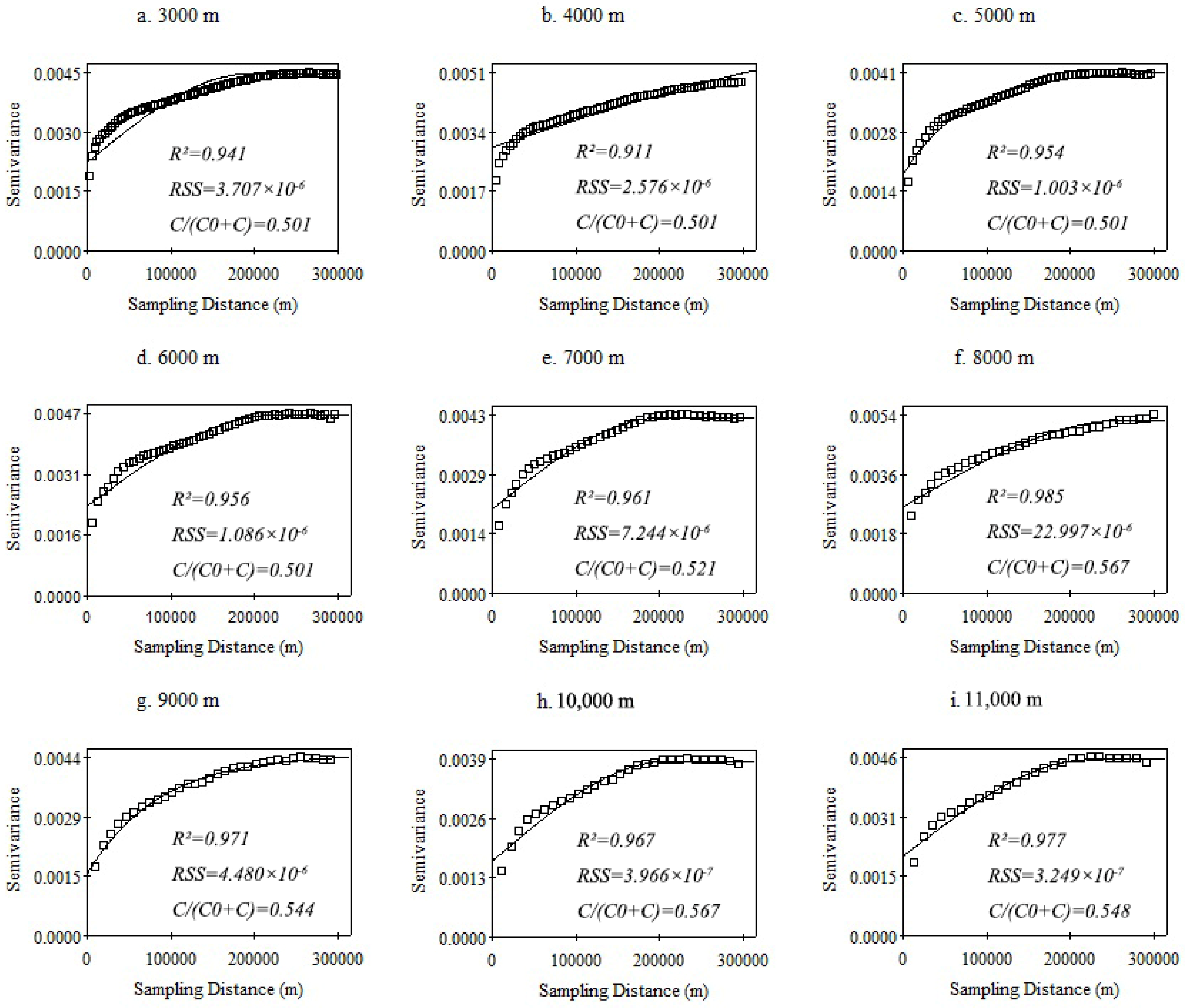
2.3.2. Semivariogram Function

The semivariogram function can characterize spatial variation and correlation patterns of regionalized variables across scales by adjusting spatial sampling intervals [60,61]. Based on semivariogram function principles, we analyzed landscape pattern indices (SHDI, AWMPFD, COHESION) under multi-scale moving windows using SVM comparison. Through scale extrapolation analysis, the optimal moving window range was determined to be 3000 m × 3000 m to 12,000 m × 12,000 m. In this study, an isotropic semivariogram model was used in GS+ 9.0 to explore the spatial structure and determine the optimal grid scale of the indicators. The isotropic model assumes that spatial variation is uniform in all directions. This assumption was selected based on preliminary data exploration, which did not reveal significant directional variation in the spatial structure. Given the regional scale of the study and the absence of strong anisotropy in the dataset, the isotropic model provides a more parsimonious and robust representation of spatial dependence. Equation (8) is as follows:
γ h = 1 2 N ( h ) i = 1 N ( h ) Z x i Z x i + h 2
where γ h is the semivariogram function of the values of the variable x at position i and position (i + h), h is the spacing distance of the sampling points (m), N ( h ) is the number of sampling points (in number) when the spacing distance is h, and Z x i and Z x i + h are landscape indices of the sampling points x i and x i + h , respectively.

2.3.3. Kernel Density Estimation

As a nonparametric estimation method, the kernel density function is widely used for analyzing spatial imbalance [62]. In this study, kernel density estimation was applied to examine the spatial evolution of ecological resilience (ER) in Jilin Province. This section is based on calculations using Stata 18 software. The calculation is given by Equation (9):
f x = 1 n h i = 1 n k ( x X i h )
where f x is the density function of ecological toughness, k is the kernel function, x is the mean value, Xi is the ecological toughness value of Jilin Province i, n is the number of grids, and h is the bandwidth; its value is related to the degree of smoothing and the density distribution, generally through the integration of the idea of minimizing the mean squared error for screening, used here to improve the accuracy of the estimation of the selection of Gaussian kernel.

2.3.4. Spatial Autocorrelation Assessment

Spatial autocorrelation evaluates attribute correlations across space using spatial statistics [63], testing whether variables correlate between adjacent regional units [64] using the Global Moran’s I index [−1, 1] to characterize overall spatial clustering patterns [65]. This section is based on calculations using GeoDa1.20 software. The calculation is given by Equation (10):
I = i = 1 n j = 1 n W i j ( Y i Y ¯ ) ( Y j Y ¯ ) i = 1 n ( Y i Y ¯ ) 2
where n denotes the total number of regional spatial units, Y i and Y j denote the attribute values of ecological toughness values on geographic units i and j, W i j is the weight matrix of the geographic units’ neighboring relationships with each other, and Y ¯ is the mean value of ecological toughness.
The LISA (Local Indicators of Spatial Association) agglomeration map was employed to analyze intra-province grid correlations and variations, characterizing the spatial structure of ecological resilience clustering patterns [49]. In the local Moran’s index results, High–High (H-H) and Low–Low (L-L) clusters indicate positive spatial autocorrelation, where grid cells with high (or low) values are surrounded by similarly high (or low) values; High–Low (H-L) and Low–High (L-H) clusters represent negative spatial autocorrelation, featuring grid cells with high (or low) values surrounded by opposing low (or high) values. The calculation is given by Equation (11):
I i = ( Y i Y ¯ ) i = 1 n ( Y i Y ¯ ) 2 · j i n W i j ( Y j Y ¯ )
where W i j is the normalized spatial weight matrix (each row sums to 1).

2.3.5. OPGD Model

The Optimal Parameters-based Geographical Detector (OPGD) model enhances the accuracy of geographical detector analysis by optimizing three key parameters: (1) spatial data discretization methods, (2) the number of spatial stratification breaks, and (3) spatial scale parameters [66]. This section is based on calculations using the R language. The calculation is given by Equation (12):
q = 1 h = 1 L N h σ h 2 / N σ 2
where h denotes the stratification level of the driver, L denotes the total number of strata, N h and σ h 2 denote the number of samples and variance of the h stratum, and N and σ 2 denote the number of samples and variance of the whole region, respectively. The range of the value of q is [0, 1], and the greater the value is, the more the driver X explains the target variable Y. The value of q is [0, 1].
The interaction detector evaluates whether the combined effects between factors enhance or diminish their explanatory power on variable Y. The risk detector identifies (1) optimal ranges and types of drivers for the dependent variable and (2) significant differences in attribute means across subdomains. The calculation is given by Equation (13):
t Y ¯ h 1 Y ¯ h 2 = Y ¯ h 1 Y ¯ h 2 V a r Y ¯ h 1 n h = 1 + V a r Y ¯ h 2 n h = 1
where Y ¯ h denotes the mean of the attribute in subregion h, nh denotes the number of samples in subregion h, and Var denotes the variance.

3. Results

3.1. Optimal Grid Scale

Considering the study area extent, average land use patch size, and ecological landscape variability, we constructed nine grid scales (from 3000 m × 3000 m to 11,000 m × 11,000 m, with 1000 m increments) based on 30 m-resolution land use raster data to assess multi-scale ecosystem adaptability (Figure 2). To ensure comparability, all the adaptability values were standardized to follow a normal distribution. Semivariogram analysis demonstrated that the nine scales exhibited strong fits under an exponential model, with determination coefficients (R2) exceeding 0.9, indicating significant spatial heterogeneity. However, the fitting accuracy varied substantially across the scales: the six finer scales (3000–8000 m) maintained superior R2 values, while the three coarser scales (9000–11,000 m) showed markedly reduced accuracy, suggesting their inadequacy for capturing ecosystem adaptability variations. Among all the scales, the 8000 m × 8000 m grid achieved optimal performance (R2 = 0.985) and was consequently selected for analyzing Jilin Province’s ecological resilience (ER) spatiotemporal evolution (2000–2020), yielding 3259 grid cells for spatial–temporal analysis. Meanwhile, the higher the nugget-to-sill ratio (C/(C0+C)), the greater the spatial heterogeneity caused by random factors. At the 3000–6000 m scale, C/(C0+C) stays stable, suggesting that the internal landscape is too simple and local patterns dominate, masking broader variations. From 7000–11,000 m, C/(C0+C) first rises then falls, indicating that as the scale increases, differences between the units shrink and spatial information is gradually lost. Therefore, based on the variation patterns of C/(C0+C), 8000 m was selected for analyzing the spatiotemporal evolution of ecological resilience (ER) in Jilin Province (2000–2020), generating a total of 3259 grid units for spatiotemporal analysis.

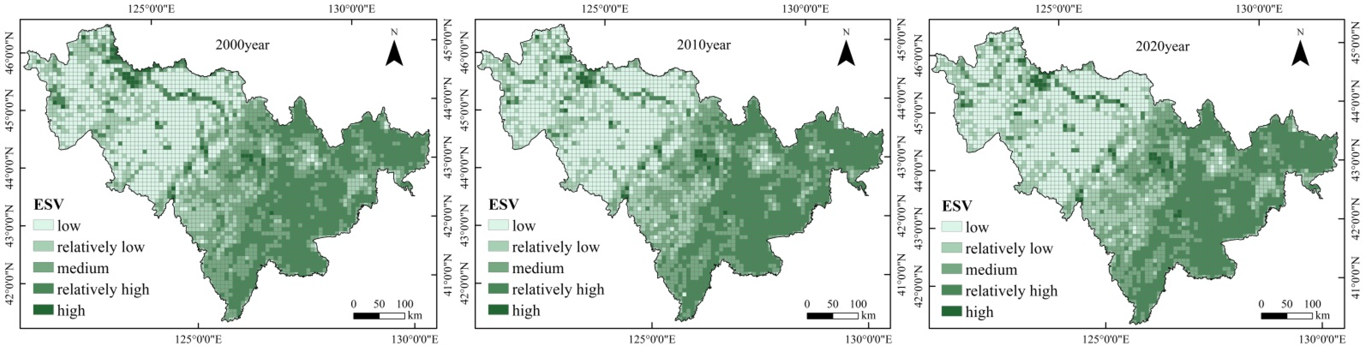
3.2. ER Spatio-Temporal Evolution

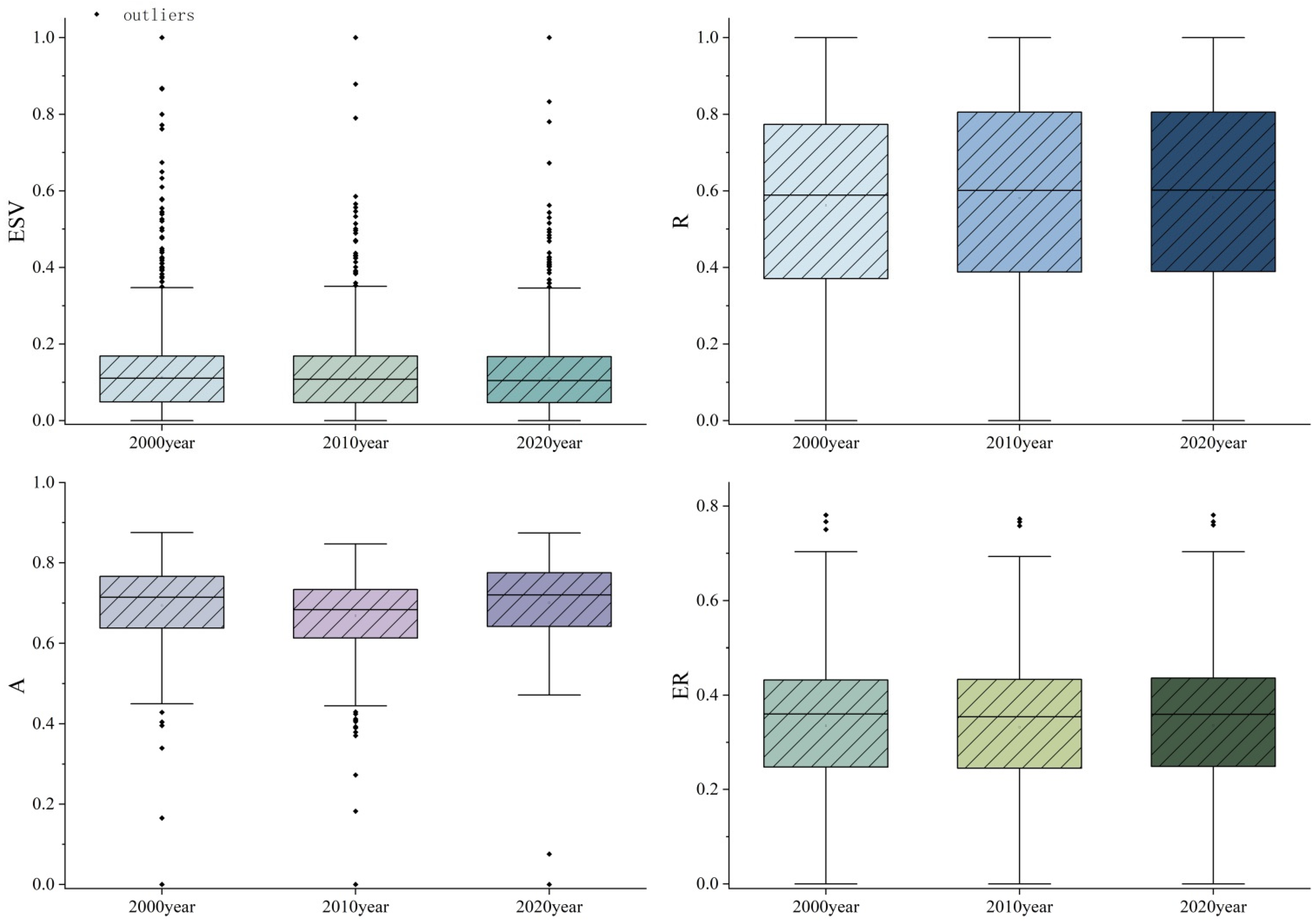
3.2.1. Ecosystem Resistance

From 2000 to 2020, the ecosystem service value (ESV) structure in Jilin Province underwent significant changes. Forest land increased substantially from 65.59% to 89.01%, becoming the dominant contributor. Conversely, water dramatically declined from 20.71% to 0.08%, while grassland decreased from 3.38% to 0.03%, indicating severe shrinkage of these ecological functions. Cropland remained relatively stable, changing marginally from 9.90% to 10.87%. These shifts demonstrate Jilin’s growing dependence on forest land for ecosystem services, with dramatically reduced contributions from water and grassland, leading to significantly diminished ecosystem diversity (Table 3).
The natural breakpoint method was used to classify ESV into five grades (Figure 3): low (0~0.06), relatively low (0.06~0.11), medium (0.11~0.16), relatively high (0.16~0.32), and high (0.32~1). Spatially, the eastern mountainous areas of Jilin Province showed a continuous distribution of high to relatively high ESV for a long period of time, and the woodland landscapes provided strong ESV; the central plains were dominated by cropland and construction types, with overall low ESV grades, especially in the urbanized core area and the distribution zone of intensive cropland, where the ESV continued to be weakened; and the western sandy fringes were dominated by low ESV, and the vulnerability of the ecosystems was relatively high. In time, from 2000 to 2010, the range of high ESV areas in the east was basically stable, but the low ESV areas in the central plains spread to the periphery with the acceleration of urbanization. From 2010 to 2020, the core area of high ESV in the east recovered slightly, low ESV in the central area showed a trend of consolidation, and the local ESV grade in the west was raised to the medium level, but the overall ESV was still dominated by the low value.

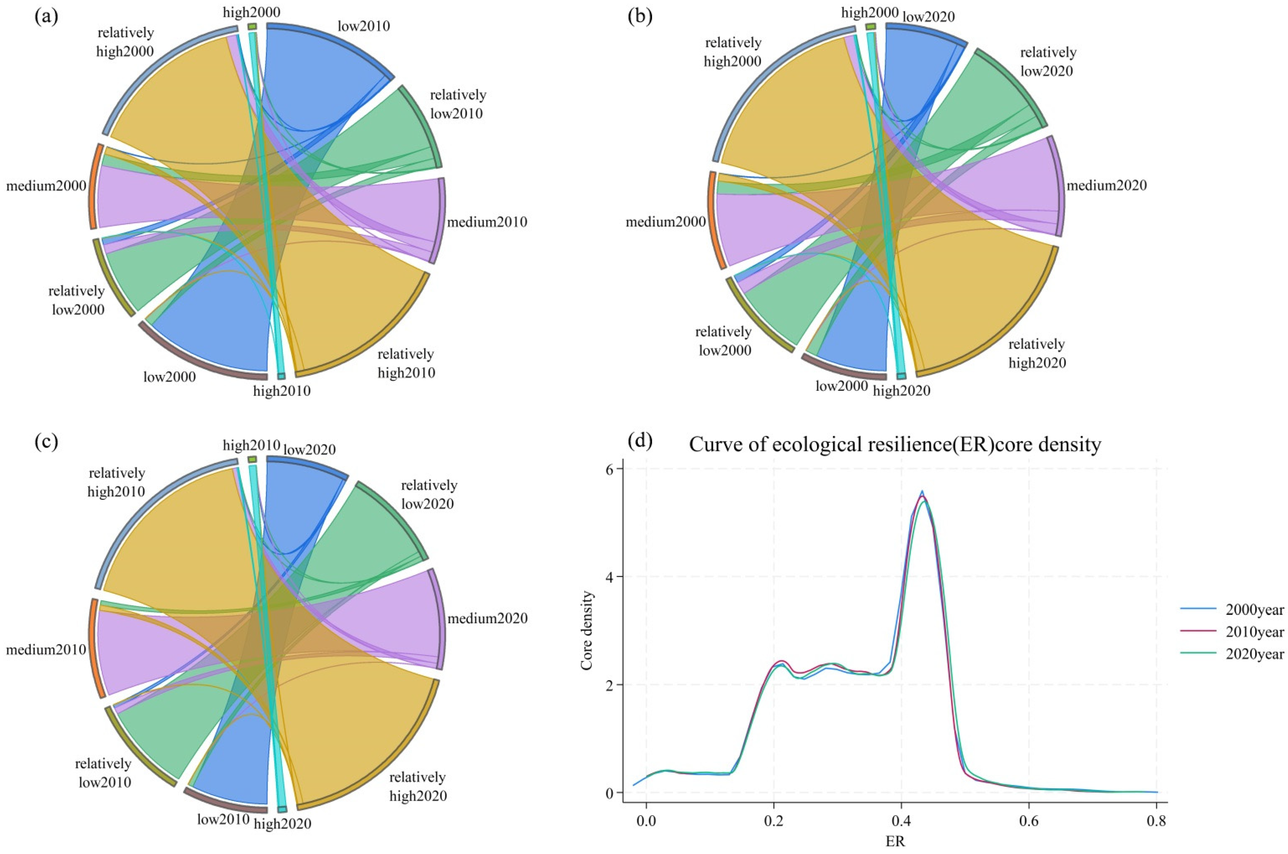
3.2.2. Ecosystem Resilience

The natural breakpoint method was used to classify R into five grades (Figure 4): low (0~0.21), relatively low (0.21~0.44), medium (0.44~0.61), relatively high (0.61~0.77), and high (0.77~1). The spatial and temporal evolution of ecosystem resilience was mapped (Figure 4). Spatially, the eastern mountainous area is characterized by a stable zone of high resilience, where the self-repairing ability of forest ecosystems provides a strong potential for recovery. The central plains are dominated by low–medium resilience, and the landscape is dominated by cropland and construction land, with the western sandy transition zone consisting primarily of sandy land. The western sandy transition zone is dominated by the transition zone of sandy land, and the landscape is predominantly made up of cropland and construction land. In the central plains, the resilience is mainly “low–medium”, and the landscape type is mainly cropland and construction land; in the western sand transition zone, the resilience is in the “low–medium” range, and the recovery threshold of salinized grassland is high, which leads to its relatively weak resilience. In time, during 2000~2010, the core area of resilience in the east remained stable, while the resilience in the central region degraded from “medium” to “low”, and the range of “low” resilience in the west further increased. The range of the “low” western resilience has further expanded; during the period 2010~2020, the resilience of some “blind zones” in the east has rebounded to the medium level, and some central regions have shown point improvements, while the resilience of the west has shown a more repeated process of change.

3.2.3. Ecosystem Adaptability

The overall change in the Ecosystem Stability Index (ESI) showed a fluctuating decline, peaking in 2010. AWMPFD, SHDI, and COHESION, the three factors affecting landscape stability, showed the most pronounced change during the study period (Table 4).
The natural breakpoint method was used to grade A, which was divided into five grades (Figure 5): low (0~0.56), relatively low (0.56~0.63), medium (0.63~0.69), relatively high (0.69~0.74), and high (0.74~1). The spatial and temporal evolution of ecosystem adaptability was summarized (Figure 5). Spatially, the eastern mountainous area is dominated by woodland, and the construction of forest roads, development of tourism facilities, and mineral exploitation have led to the fragmentation of forest patches, and the adaptability level is maintained at “low–relatively low”. The central region is dominated by cropland, and large-scale mechanized farming in the Songnen Plain has formed a continuous cropland landscape with a strong anti-disturbance response capacity. The ecosystem adaptability is mainly concentrated in the “relatively high–high” levels and has the stability characteristics of a high-intensity cropland landscape. Water resources in the study area are primarily located in the western part of the country, and due to the fragility of the western ecosystem, result in a large area of “relatively high–high” class distribution. From 2000 to 2010, the area of the “low–relatively low” adaptability zone in the central and western regions increased due to rapid urbanization and agricultural expansion, while the area of the high adaptability zone in the eastern region remained basically stable; from 2010 to 2020, the area of high adaptability zone in the eastern mountainous region slightly expanded. Between 2010 and 2020, high adaptability expanded slightly in the eastern mountains, a minor rebound occurred in the central region, and localized adaptability rose in the west.

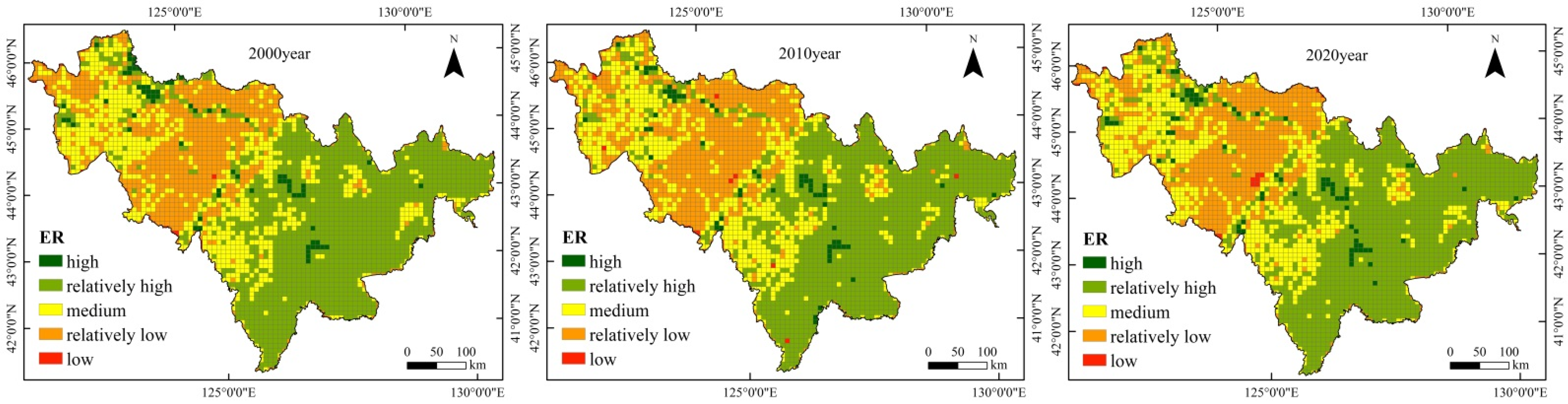
3.2.4. Ecological Resilience

The natural breakpoint method is used to classify the ER into five grades (Figure 6): low (0~0.14), relatively low (0.14~0.27), medium (0.27~0.38), relatively high (0.38~0.50), and high (0.50~0.80), and the distribution pattern of ER is stable from 2000 to 2020, forming an “east–high, west–low” map of ER. Spatially, medium and low ER dominate the landscape, covering the central and western plains and the wind–sand transition zone in a basal shape, dominated by cropland, salinized grassland, and unused land, reflecting the superposition of agricultural intensification and ecological vulnerability; low ER is mainly located in the central urban area, with a smaller area, and positively correlates with the expansion of construction land. The central low ER is dominated by contiguous cropland with a fragmented landscape, reducing ecological connectivity and ecological vulnerability; the western low ER is dominated by salinized grassland and sandy land, with infertile soils, sparse vegetation, and an extremely weak natural restoration ability. The medium ER is distributed in the intertwined zones of cropland and woodland and around the irrigation area and artificial management area, and it has formed localized ecological vulnerability through the protection of a small area of wetland. Relatively high ER is mainly distributed in the eastern forest belt of Changbai Mountain, with natural forests and wetland landscapes dominating the area. High ER is mainly distributed in the watersheds of Jilin Province, such as the Songhua River in the east-central part of the province and the Xianghai Wetland in the western part of the province, with a belt-type or patch-type distribution, which has significantly increased the regional resistance to disturbances and the ability to recover.
The boxplots (Figure 7) show the trends of the four variables ESV, R, A, and ER between 2000, 2010, and 2020. Among them, the median of ESV decreased slightly and there were more outliers in 2000 and 2010: the median of R showed an increasing trend, especially between 2000 and 2010, which increased significantly; the median of A showed a decreasing and then an increasing trend, with a more significant increase; and there was a decreasing trend in the median of ER, which decreased significantly between 2000 and 2020. Overall, R and A show an increasing trend, while ESV and ER show a slight decreasing trend.
When calculating the 2000-2020 ER transition chord diagram and kernel density analysis (Figure 7), Figure 8a–c show the transfer chord diagrams of ER levels in Jilin Province for the periods of 2000~2010, 2000~2020, and 2010~2020, respectively, where the width of the chord indicates the transfer intensity and the colors represent different ER levels. Generally speaking, Jilin Province is dominated by relatively high ER, with a small amount of mutual transfer between the different levels. In 2000~2010, low ER areas dominated the overall transfer process, and the ER basically maintained the status quo ante; medium ER areas were highly stabilized, and only a small amount of high ER areas were degraded. In 2010~2020, the low ER areas showed a trend of solidification. The ER areas showed a solidifying trend, the high ER areas became more stable, and the relatively high ER areas increased slightly. From 2000 to 2020, the ER showed a decreasing trend, the low ER and relatively low ER areas increased significantly, and the medium ER areas acted as a core hub and played a connecting role between different classes, while high ER areas degraded slowly. Figure 8d shows the kernel density curves of ER in 2000, 2010, and 2020. The overall position of the curves does not change much, and the shifting range is relatively small, indicating that the main ER level in Jilin Province is basically stable. The kernel density curves in each year are bimodal, with the main peak located in the relatively high ER zone and the secondary peak in the relatively low ER zone, showing obvious polarization. The right side of the curve always has a trailing tail, indicating that the high ER region is small in proportion but stable. The change of the wave peaks shows that it firstly rises and then decreases; the distribution area firstly shrinks and then expands, reflecting that the difference of the ER increased in the period of 2000~2010 and the difference of the ER in the period of 2010~2020 increased. The wave peaks first rise then fall, and the distribution area first shrinks then expands, showing that ER differences intensified from 2000 to 2010 and eased slightly from 2010 to 2020. The ER index at the main peaks remains around 0.42, with the secondary peak near 0.21. Small changes in density values confirm the stable spatial pattern and long-term significance of ER differences in Jilin Province.

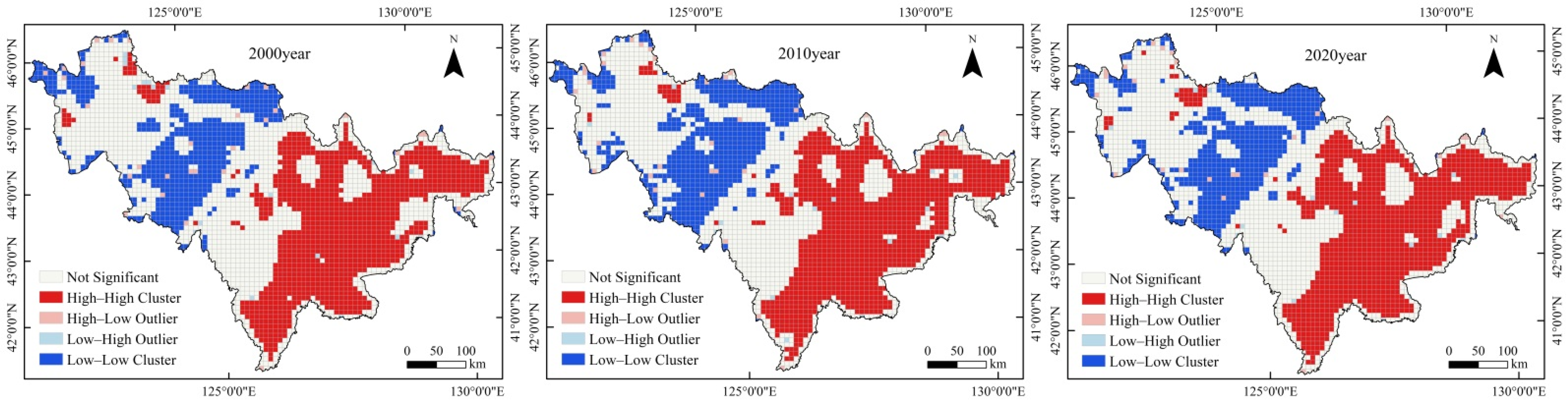
3.2.5. Spatial Autocorrelation Analysis

The Global Moran’s I index (Figure 8) of ER in Jilin Province from 2000 to 2020 was calculated in order to analyze the overall spatial clustering characteristics of ER in the spatio-temporal dimension. The results show that Moran’s I index remains above 0.5 every year, and the p-value is less than 0.01, indicating that the ER of Jilin Province shows significant positive spatial autocorrelation and obvious spatial clustering characteristics during the study period.
Further analysis of the LISA clustering diagram (Figure 9) reveals that ER in Jilin Province generally follows a consistent spatial pattern, mainly dominated by the “high–high” and “low–low” types of agglomeration, showing significant regional polarization characteristics. The distribution of “low–high” and “high–low” heterogeneous agglomerations is small and limited. The “high–high” type is primarily located in the mountainous forest areas in the eastern part of Jilin Province, where the ecological background conditions are good, and the ecosystems have strong resistance and resilience and are the core advantageous areas of ER in the province, particularly in the Changbai Mountain region. This area has high elevation and steep slopes, providing excellent ecological conditions. It is also home to large areas of mixed coniferous and broadleaf forests and natural secondary forests, which exhibit high biodiversity and strong ecosystem self-regulation capabilities. Additionally, the eastern part of the region contains several national and provincial-level nature reserves (such as the Changbai Mountain National Nature Reserve and the Hunchun Northeast Tiger and Leopard National Park), with relatively well-established ecological protection policies and regulatory mechanisms. Furthermore, national ecological projects, such as the Grain-for-Green Program and the Three-North Shelterbelt Forest Program, have been implemented with significant intensity in this region. These factors collectively enhance the ecosystem’s ability to withstand disturbances and recover.
The “low–low” area is mostly distributed in the central and western plains, which is dominated by cropland, construction land, and unused land and is strongly disturbed by human activities, with fragile ecosystems and generally low resistance and resilience. From 2000 to 2020, with the continuous implementation of ecological projects and ecological protection efforts continuing to increase, the eastern mountainous region of the “high–high” agglomeration area gradually expanded, and the ecological advantages of the area to enhance ER. The central plain region is the main agricultural production area of Jilin Province, represented by Songyuan, Changchun, and Siping. It has a high proportion of arable land, a highly monotonous land use pattern, a simple ecosystem type structure, and weak regulatory capacity. Additionally, this region serves as the provincial hub for population and industrial concentration. In recent years, urban expansion has accelerated, leading to rapid growth in construction land. Intensive land use has significantly compressed natural ecological spaces, resulting in pronounced fragmentation of ecological patches and a concurrent decline in both the resilience and resistance of ecosystems. Furthermore, the region’s heavy reliance on water resources for agricultural activities makes its ecosystems vulnerable to droughts, floods, and human disturbances. This results in high sensitivity to climate change but low adaptability, leaving ecological resilience in a state of high volatility. The western region is located in a semi-arid climate zone and is one of the most ecologically fragile areas in Jilin Province. Due to natural constraints, the region has scarce precipitation, high evaporation rates, and limited surface water resources. Its ecosystems primarily consist of grasslands, desertified lands, and partially degraded wetlands, with low biological productivity. The region faces extensive issues with saline–alkali soils and desertification, resulting in severe soil degradation. Although ecological governance projects have been implemented in recent years (such as the Korqin Desert Governance Project and the Grain-to-Grassland Conversion Program), the fragile baseline conditions of the ecosystems make it difficult to significantly enhance overall ecological resilience in the short term. Additionally, some areas in the region have long relied on resource-based industries (such as wind power and mining), leading to prominent conflicts between development and conservation, making it challenging to achieve a benign ecological cycle and stable succession.
In summary, the spatial differentiation of ecological resilience in Jilin Province is not only influenced by natural geographical conditions but is also closely related to regional development models, land use structures, and policy support. At the same time, the intensification of agricultural management and the urbanization acceleration have led to the expansion of “low–low” areas in the central and western regions, and the pattern of ecological differentiation has become more obvious. Overall, the ER in Jilin Province is characterized by a spatial pattern of “high in the east and low in the west”, and the imbalance of regional development still exists. (See Figure 10).

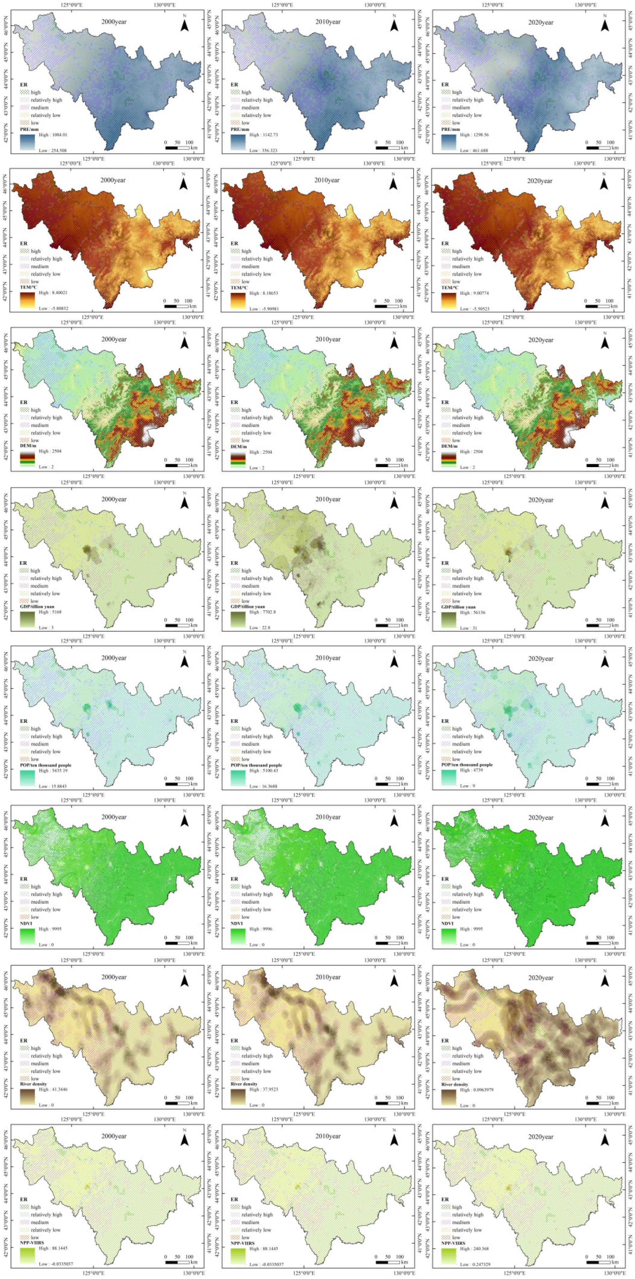
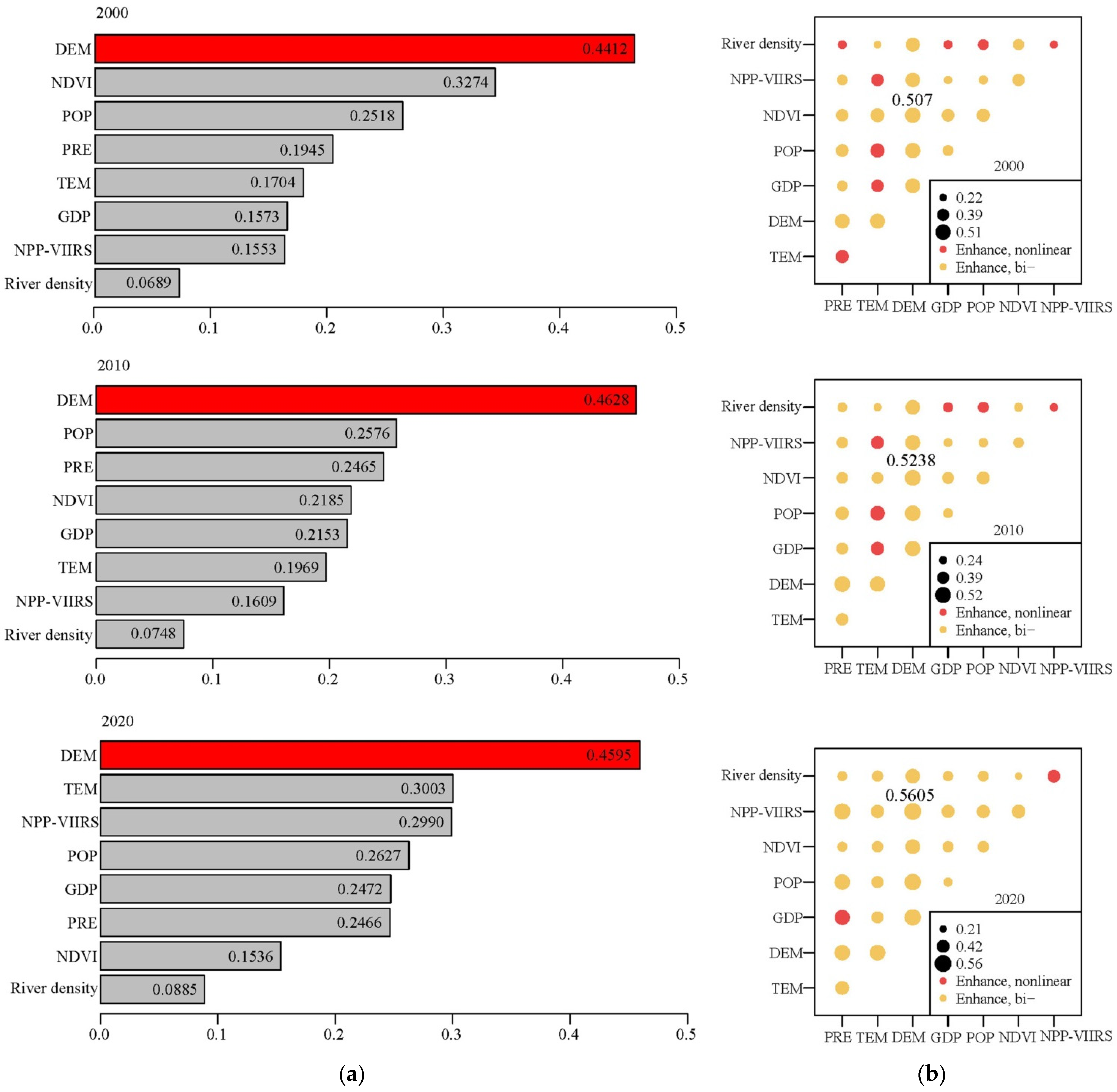
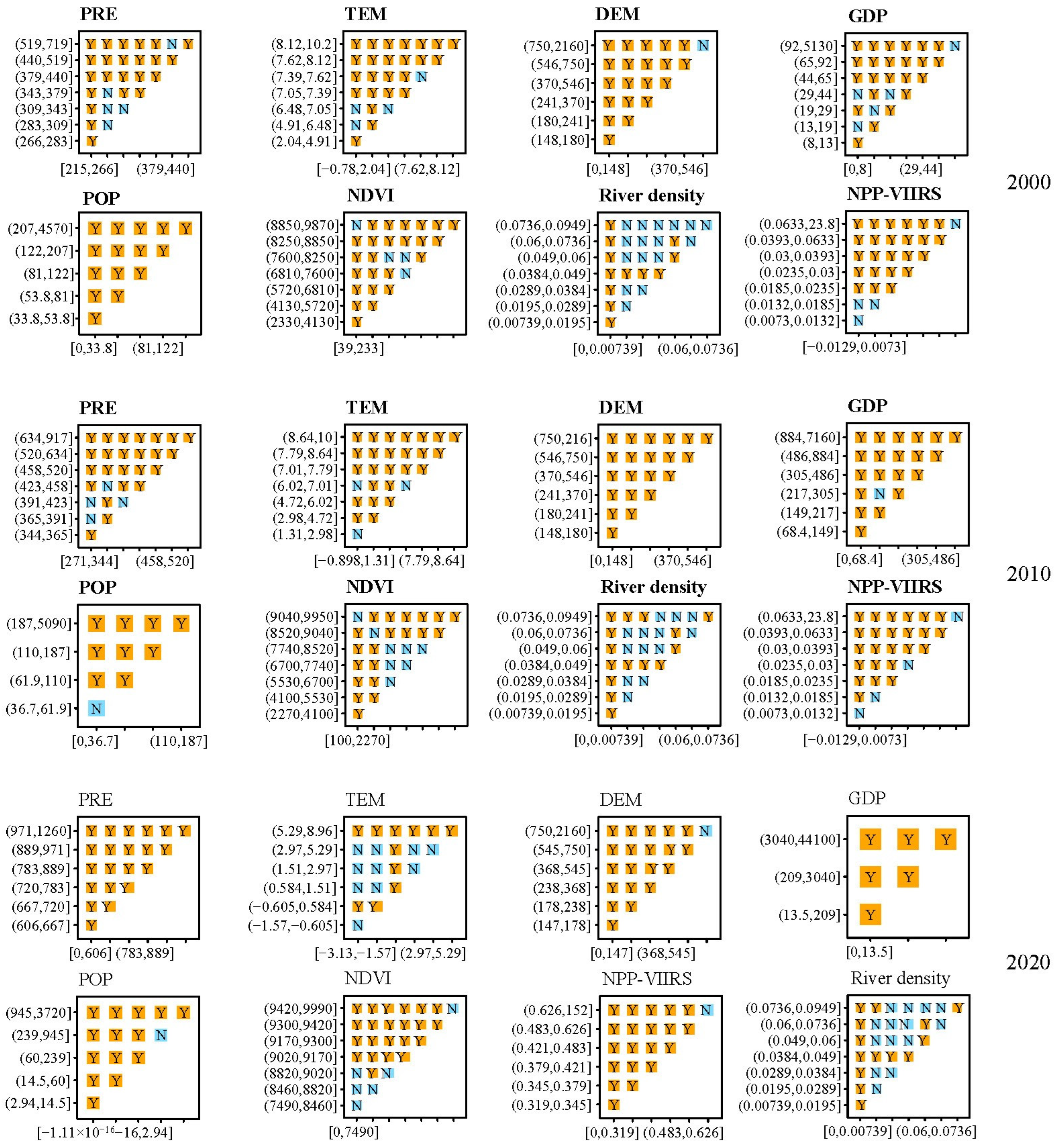
3.3. Identification of Influencing Factors

From the perspectives of society, economy, and nature, considering regional conditions and grid scale, eight driving factors—PRE, TEM, DEM, GDP, POP, NDVI, NPP-VIIRS, and river density—were selected to analyze the dominant factors in Jilin Province at different times (Figure 11).
The OPGD model was used to systematically analyze the influence of eight factors on ER to reveal the main drivers of ER changes in Jilin Province (Figure 12a). In the single-factor analysis, DEM was consistently the most important factor influencing ER in 2000, 2010, and 2020, with values stabilizing between 0.44 and 0.46. The importance of NDVI declined over time, dropping from second place in 2000 to seventh in 2020. Meanwhile, the influence of POP, GDP, TEM, and NPP-VIIRS increased significantly. In 2020, TEM and NPP-VIIRS became the next most important factors, reflecting the combined effects of climate change and intensified human activities. In contrast, river density always had the smallest impact, but the value increased slightly. Overall, the drivers of ER gradually evolved from natural dominance in the early stage, such as DEM and NDVI, to a pattern of combined natural and anthropogenic factors, such as POP, GDP, and NPP-VIIRS.
The synergistic effect of environmental factors on ER continuously increased between 2000 and 2020 (Figure 12b). The q-value of this interaction rose significantly from 0.507 in 2000 to 0.5605 in 2020. This synergy consistently exhibited a significant nonlinear enhancement effect. The explanatory power of this synergy far exceeds the independent effects of each single factor, with the interactive combination of climate (PRE, TEM), topography (DEM), and socio-economic factors (GDP, POP) showing the strongest synergistic effect. Meanwhile, the synergistic effect between the socio-economic factors and the NPP-VIIRS data characterizing human activities in 2020 is particularly prominent, reflecting the continuous intensification of the impacts of human activities on the ecological environment in the process of rapid urbanization. The interaction between the NDVI and the river density is relatively weaker, but the synergistic effect between it and the climatic factors is still not to be neglected. In summary, the driving mechanism of ER is essentially a complex multi-factor nonlinear synergistic process, and the coupling effect of natural environmental elements and human socio-economic activities must be taken into account in ecological environment management, especially the interaction effect between climate, topography, and human activities.
The spatial distribution of ER across the range of drivers (Figure 13) demonstrates the characteristics of spatial differentiation of ER by different drivers and its evolution pattern during 2000–2020. In terms of climate factor combinations, regions with high temperatures and high precipitation generally exhibit lower ecological resilience. This was particularly evident in 2020, when extreme climate conditions led to a significant decline in ecological resilience, reaching its lowest point. This indicates that under conditions of increased climate variability, the ecosystems’ ability to adapt to extreme weather events has significantly decreased, demonstrating a clear “climate stress threshold effect.” This is closely related to the destructive impact of extreme high temperatures combined with abnormal precipitation on ecosystem stability, species diversity, and soil and water conservation functions. In terms of socio-economic factor combinations, regions with high GDP and high population density exhibit an exponential decline in ecological resilience, reaching the lowest level in 2020. This result highlights the profound impact of human activity intensity on ecosystem structure and function. Intensive economic development and rapid urbanization may lead to high-intensity land use, water resource shortages, and ecological space compression, thereby causing composite disturbances to ecological resilience, reflecting a clear “cumulative effect”; in the natural–human composite driving combination, when terrain (high DEM) and human activities (NPP-VIIRS) interact, ecological resilience shows a significant improvement, far exceeding the scenario of single-factor influence. This suggests that there may be a synergistic effect between the baseline characteristics of natural conditions and moderate human development, manifested as a “coupling enhancement mechanism,” where moderate development under certain natural constraints may actually enhance system stability. The NDVI factor exhibits a notable regulatory role: high NDVI regions can effectively mitigate the negative impacts of other disturbance factors on ecological resilience, indicating that vegetation cover plays an important protective and restorative role in ecosystems. In contrast, regions with moderate NDVI exhibit a decline in ecological resilience accumulation, which is associated with factors such as unstable vegetation cover and marginalized land use, reflecting the risk of “moderate disturbance accumulation.” In the combination of river density and NPP-VIIRS, ecological resilience exhibits a distinct nonlinear characteristic. High river network density combined with high human activity areas form distinct ER hotspots, particularly evident in 2020. This nonlinear synergistic effect is due to the attractiveness of water bodies to human settlements, while excessive development of water-adjacent areas exacerbates ecosystem vulnerability, reflecting the characteristics of a “resource-development coupling sensitivity zone.”
Overall, ecological resilience is driven by multiple factors, with its variation patterns exhibiting significant nonlinearity and interactive enhancement effects. Especially in 2020, ecological resilience in regions where multiple factors converge reached peak or trough values, indicating that ecosystem stability faces greater challenges under the combined influence of climate variability and human activities.
The ER matrix analysis in Figure 14 shows the spatial distribution characteristics of ER under different combinations of driving factors. The spatial variation of ecological resilience risks in Jilin Province is driven by both natural and human factors. The extent of the influence and temporal variation characteristics of different factors can be analyzed using the risk detector results of the OPGD model. A significant marker “Y” indicates that the factor’s stratification interval has a statistically significant explanation for risk, while “N” indicates no significant impact. The analysis shows that PRE, DEM, POP, and NPP-VIIRS are stable driving factors for ecological risk. PRE was significantly significant (Y) in most intervals between 2000 and 2020, indicating that its spatial variations have a sustained impact on ER, potentially related to flood or drought risks caused by uneven precipitation distribution in Jilin Province. Almost all the stratification intervals of DEM are marked as “Y,” highlighting the foundational regulatory role of different landform units (e.g., mountains, plains) in ecosystem stability. Among the human factors, high-value intervals of POP and NPP-VIIRS are generally significant, reflecting more pronounced ecological pressures in areas with concentrated human activities (e.g., urban agglomerations). In contrast, the influence of economic level (GDP) shows a phased weakening, with only the medium-to-low economic level intervals remaining significant in 2020, suggesting that economic development may mitigate some ecological risks through technological or management measures. The significance of TEM and NDVI fluctuates over time, with some intervals turning to “N” in 2020, which may be related to the increase in extreme temperature events or dynamic changes in vegetation cover under the backdrop of climate change. River density contributes weakly overall (mostly “N”), with only localized intervals showing significance, indicating that its impact is spatially limited. In summary, the formation mechanism of ecological resilience risks in Jilin Province is primarily dominated by natural foundations (climate, topography), with human activities (urbanization, economic development) playing a reinforcing or regulating role. Future risk management should prioritize the interactive effects of precipitation and topography, optimize ecological space planning in high population density areas, and dynamically monitor the threshold effects of climate-sensitive factors (such as temperature and vegetation). Additionally, the weakened explanatory power of economic levels suggests the effectiveness of policy interventions (such as ecological compensation), which could serve as a potential breakthrough for enhancing regional resilience.

4. Discussion

4.1. Characterization of ER Spatio-Temporal Evolution and Analysis of Driving Factors

Long-term uncontrolled resource development in Jilin Province has caused a decline in the water table and increased the risk of water resource depletion. In areas like the Songnen Plain, soil salinization has severely impacted agricultural production and the ecological environment. Additionally, over-exploitation and irrational land use have resulted in land degradation and reduced ecosystem service functions. These environmental problems not only threaten the ecological security of Jilin Province but also directly affect agricultural production and sustainable socio-economic development. Therefore, it is of great practical significance to study the changes of ER and its spatial and temporal evolution patterns in various regions of Jilin Province. Based on this, this study aims to analyze the key indicators of ER in Jilin Province, such as resistance, resilience, and adaptability, to explore the differential performance of different regions in coping with environmental pressures (Figure 15) and to assess the stability and restoration potential of ecosystems in each region.
The long-term high ecosystem service value (ESV) in eastern Jilin’s mountainous areas is mainly due to woodland protection and stable ecological functions. The dominance of forest ecosystems contributes to the region’s high ecological resistance. In contrast, the central plains, especially the core area with rapid urbanization and the agricultural belt, have lower ESV levels and gradually weakened ecosystem resistance, indicating that the ecological function of the region has been significantly and negatively affected. In contrast, the western sandy fringe area also had lower ESV, showing higher ecological vulnerability. The eastern mountainous areas of Jilin exhibit strong ecosystem resilience, mainly because of the forest ecosystems’ self-repair ability and favorable ecological conditions. On the contrary, the central plains and western sandy areas, especially salinized grasslands and sandy areas, have lower resilience and show stronger ecological vulnerability. In terms of ecosystem adaptability, the eastern mountainous areas show high ecological adaptability, indicating that the ecosystems of the region exhibit high stability and adaptability in the face of environmental pressures. In the central region, ecological adaptability is generally low due to the high intensity of land development and the high proportion of cropland and construction land. The western region is also less adaptable due to its fragile ecological structure, and the ecosystems have difficulty responding effectively to environmental pressures.
In terms of the spatial and temporal distribution of ER, low to medium ER areas dominate the plains and sandy transition zones in the central and western parts of Jilin Province. Agricultural intensification and the expansion of salinized grasslands have increased the ecological vulnerability of these areas. High ER areas in the eastern mountainous regions mainly include natural forests and wetlands, which have good ecological connectivity and strong water storage capacity. Watersheds in Jilin Province also exhibit high ER and play key roles in hydrological regulation, habitat maintenance, and pollution purification. Temporally, from 2000 to 2010, low ER areas in central and western Jilin Province increased significantly, reflecting pressures from agricultural intensification and urbanization. From 2010 to 2020, the eastern province maintained high ER through forest protection, and some saline management areas in the west showed improved resilience. However, the overall pattern of “high in the east and low in the west” persisted. The overall pattern remains “high in the east and low in the west”. ER continues to decline in the central region as a result of urbanization and agricultural intensification.
Based on the OPGD model, the driving mechanism of ER and its spatio-temporal evolution pattern from 2000 to 2020 were systematically revealed through single-factor detection, interaction detection, and risk matrix analysis. The single-factor analysis showed that DEM consistently remained the most important driver, with its influence stabilizing between 0.44 and 0.46. Meanwhile, the importance of NDVI continued to decline, and the influences of TEM and NPP-VIIRS were significantly enhanced, reflecting the increasingly prominent impacts of climate change and human activities. The interaction detection results indicate a continuous strengthening of synergistic effects among the factors, with the q-value rising from 0.507 in 2000 to 0.5605 in 2020. This synergy is mainly characterized by a nonlinear enhancement effect in which the interactions between the climate factors (PRE, TEM), the terrain factor (DEM), and the socio-economic factors (GDP, POP) are particularly significant, especially the interaction between the socio-economic factors and the nighttime lighting data in 2020, which is particularly significant. The synergistic effect of socio-economic factors with NPP-VIIRS in 2020 highlights the key impacts of human activities. The ER matrix analysis further validated these findings, with high-temperature and high-precipitation regions, such as PRE and TEM, as well as the high-GDP and high-POP intervals (GDP 3040~44,100, POP 945~3720). The number and intensity of high-ER combinations increased significantly in 2020, and the ER value of the climate–economy composite combination especially increased nearly three times compared with that in 2000, indicating that the regional ecological ER pattern has entered a new stage of “multi-factor synergistic amplification”. Together, these results indicate that the formation of contemporary ER is the result of complex interactions between natural factors and human activities and that such interactions are increasing. Therefore, future ecological risk management needs to adopt a comprehensive strategy, focusing on key geographical areas, such as climate variability-sensitive areas, high-intensity human activity concentration zones, and natural–human transition zones, in order to realize the goal of regional sustainable development.
Based on the spatial distribution characteristics of ecological resilience and differences in dominant driving factors, this paper divides Jilin Province into three ecological resilience management zones and proposes corresponding strategy recommendations. The Ecological Conservation Priority Zone is mainly located in the eastern Changbai Mountain region. This zone features good ecological conditions, high forest coverage, and stable ecosystems. It is recommended to strengthen nature reserve management, strictly control human interference, and promote sustainable forestry along with ecological red line protection. The Ecological Restoration and Enhancement Zone covers the central Songliao Plain, an important agricultural area where ecosystems have been significantly disturbed but still have restoration potential. Measures such as crop rotation, ecological corridor construction, and green agriculture development are advised to improve ecological service functions. The Ecological Governance Vulnerable Zone is concentrated in the western arid and saline–alkali regions, including Baicheng, where ecological degradation is severe. Strengthening ecological monitoring and risk warning systems, implementing comprehensive projects like returning farmland to grassland and desertification control, and promoting adaptive ecological industries are recommended. By implementing classified and zoned management, the overall ecological resilience of Jilin Province can be improved, thereby supporting regional ecological security and sustainable development.

4.2. Suggestions for Countermeasures

According to the results of the spatial and temporal evolution of ER and the analysis of influencing factors, the future development of Jilin Province can focus on the following aspects:
Strengthen ecological protection and restoration efforts in the Changbai Mountain region and surrounding ecological functional zones in the eastern part of the country. Designate the Changbai Mountain Nature Reserve, Hunchun Forest Area, and Dunhua-Antu Forest Area as key ecological protection zones, establish strict ecological protection red lines, prohibit excessive development, and ensure the sustainable use of forest resources. Advance the Natural Forest Conservation Program to eliminate illegal logging. For areas that have already been damaged, particularly in severely eroded areas, such as the southwestern part of Tonghua City, the western edge of Baishan City, and the border region between Hui Nan and Jia An, implement systematic ecological restoration projects. This should be achieved through measures such as soil and water conservation and converting farmland back to forests to restore the ecological functions of these regions.
Upgrade eco-agriculture and coordinated urban–rural development in the central region and implementing more refined eco-agriculture strategies and coordinated urban-rural development. In urban and rural development, promote the construction of green infrastructure, such as urban parks, green belts, and water systems, to enhance ER. At the same time, this strengthens the sharing of ecological resources and promotes positive interaction between urban and rural areas; this also leads to the adoption of diversified land use methods and avoids a single land development model.
Optimize ecological restoration and land management in the western region, restoring ecological functions and reducing wind and sand disasters and soil erosion through large-scale vegetation restoration, sand-barrier construction, and saline–alkali land improvement techniques. Focusing on the efficient use and protection of water resources has strengthened soil and water conservation projects, optimized the allocation of water resources, and developed water resource recycling techniques to ensure the supply of water resources for ecological restoration in the west.

4.3. Limitations and Future Improvements

This study faces several limitations. First, the land use data (CNLUCC) is only updated to 2020, which may limit the timeliness of the conclusions. Future research will incorporate high-temporal-resolution datasets and annual monitoring products to improve accuracy. Second, the assessment framework relies on a single indicator, leading to a lack of comprehensive ecological validation. Future work should integrate multiple indicators and consider socio-economic and governance factors. Third, the simulation results are based on assumptions that may not fully capture future policy or environmental changes. Uncertainty analysis and multi-scenario simulations will help address this. Finally, the focus on Jilin Province limits the broader applicability of the results. Expanding the study area and incorporating comparative analysis will enhance generalizability.

5. Conclusions

This study analyzed changes in ecosystem adaptability using scale extrapolation and multi-scale grid data integration. The spatial and temporal evolution of ER in Jilin Province was analyzed at a scale of 8000 m. Using 3259 grid cells, this study examined the dynamics of resistance, resilience, adaptability, and overall ER in Jilin Province from 2000 to 2020. The main conclusions are as follows:
Spatially, the polarization “high east, low west, and central pressure” characteristics are presented, with the ER of the forested areas in the east being stable, and the ER of the central and western areas being generally low due to significant interference from human activities. In time, from 2000 to 2010, the overall ER declined, and the low ER areas in the central and western regions expanded; from 2010 to 2020, local restoration measures (such as wetland restoration and construction of protective forests) made some areas of ER rebound, but the overall pattern has not been fundamentally changed.
Through spatial autocorrelation analysis, the ER of the eastern mountainous areas of Jilin Province was higher during the study period, and the ecological advantage of the eastern part of the province was expanded, mainly concentrated in the “high–high” aggregation area. The central and western plains, on the other hand, show low ER, mainly in the “low–low” agglomeration area, and the phenomenon of ecological differentiation is becoming increasingly obvious.
DEM remained the most stable factor influencing ER. The impact of NDVI weakened over time, while the influence of temperature (TEM) and nighttime light (NPP-VIIRS) increased significantly. The synergistic effect among the factors showed a clear upward trend, with the interaction q-value rising from 0.507 in 2000 to 0.5605 in 2020. The interaction between climatic (PRE, TEM) and socio-economic factors (GDP, POP) was the most prominent. By 2020, high-ER areas had expanded significantly, and the ER value driven by the climate–economy combination was nearly three times higher than in 2000. Areas with high NDVI demonstrated strong ER buffering capacity.

Author Contributions

Conceptualization, Y.Z. (Yuqi Zhang); methodology, Y.Z. (Yuqi Zhang); formal analysis, Y.Z. (Yuqi Zhang); data curation, Y.Z. (Yuqi Zhang) and Y.Z. (Yue Zhu); writing—original draft, Y.Z. (Yuqi Zhang); writing—review and editing, Y.Z. (Yuqi Zhang) and J.L.; funding acquisition, J.L. and Y.Z. (Yue Zhu). All authors have read and agreed to the published version of the manuscript.

Funding

This research was funded by the National Natural Science Foundation of China (41977411); the Science and Technology Development Programme of Jilin Province (YDZJ202501ZYTS492); and the Jilin Provincial Department of Education (JJKH20240563CY).

Data Availability Statement

The original contributions presented in this study are included in the article. Further inquiries can be directed to the corresponding author.

Conflicts of Interest

The authors declare no conflicts of interest.

References

  1. Zhu, S.; Kong, X.; Jiang, P. Identification of the human-land relationship involved in the urbanization of rural settlements in Wuhan city circle, China. J. Rural Stud. 2020, 77, 75–83. [Google Scholar] [CrossRef]
  2. Kassouri, Y. Monitoring the spatial spillover effects of urbanization on water, built-up land and ecological footprints in sub-Saharan Africa. J. Environ. Manag. 2021, 300, 113690. [Google Scholar] [CrossRef] [PubMed]
  3. Li, S.; Wu, J.; Gong, J.; Li, S. Human footprint in Tibet: Assessing the spatial layout and effectiveness of nature reserves. Sci. Total Environ. 2018, 621, 18–29. [Google Scholar] [CrossRef] [PubMed]
  4. Xu, C.; Li, B.; Kong, F.; He, T. Spatial-temporal variation, driving mechanism and management zoning of ecological resilience based on RSEI in a coastal metropolitan area. Ecol. Indic. 2024, 158, 111447. [Google Scholar] [CrossRef]
  5. Martin, R. Regional economic resilience, hysteresis and recessionary shocks. J. Econ. Geogr. 2012, 12, 1–32. [Google Scholar] [CrossRef]
  6. Rose, A. Economic resilience to natural and man-made disasters: Multidisciplinary origins and contextual dimensions. Environ. Hazards 2007, 7, 383–398. [Google Scholar] [CrossRef]
  7. Holling, C.S. Resilience and stability of ecological systems. Annu. Rev. Ecol. Syst. 1973, 4, 1–23. [Google Scholar] [CrossRef]
  8. Nie, C.; Lee, C.-C. Synergy of pollution control and carbon reduction in China: Spatial–temporal characteristics, regional differences, and convergence. Environ. Impact Assess. Rev. 2023, 101, 107110. [Google Scholar] [CrossRef]
  9. Worstell, J. Ecological resilience of food systems in response to the COVID-19 crisis. J. Agric. Food Syst. Community Dev. 2020, 9, 23–30. [Google Scholar] [CrossRef]
  10. Li, H.; Wang, Y.; Zhang, H.; Yin, R.; Liu, C.; Wang, Z.; Fu, F.; Zhao, J. The spatial-temporal evolution and driving mechanism of Urban resilience in the Yellow River Basin cities. J. Clean. Prod. 2024, 447, 141614. [Google Scholar] [CrossRef]
  11. Li, G.; Wang, L. Study of regional variations and convergence in ecological resilience of Chinese cities. Ecol. Indic. 2023, 154, 110667. [Google Scholar] [CrossRef]
  12. Wang, J.; Wang, J.; Zhang, J. Spatial distribution characteristics of natural ecological resilience in China. J. Environ. Manag. 2023, 342, 118133. [Google Scholar] [CrossRef] [PubMed]
  13. Zhang, T.; Sun, Y.; Zhang, X.; Yin, L.; Zhang, B. Potential heterogeneity of urban ecological resilience and urbanization in multiple urban agglomerations from a landscape perspective. J. Environ. Manag. 2023, 342, 118129. [Google Scholar] [CrossRef] [PubMed]
  14. Zhao, R.; Fang, C.; Liu, H.; Liu, X. Evaluating urban ecosystem resilience using the DPSIR framework and the ENA model: A case study of 35 cities in China. Sustain. Cities Soc. 2021, 72, 102997. [Google Scholar] [CrossRef]
  15. Abdi, R.; Rogers, J.B.; Rust, A.; Wolfand, J.M.; Philippus, D.; Taniguchi-Quan, K.; Irving, K.; Stein, E.D.; Hogue, T.S. Simulating the thermal impact of substrate temperature on ecological restoration in shallow urban rivers. J. Environ. Manag. 2021, 289, 112560. [Google Scholar] [CrossRef]
  16. Folke, C. Resilience: The emergence of a perspective for social–ecological systems analyses. Glob. Environ. Change 2006, 16, 253–267. [Google Scholar] [CrossRef]
  17. Capdevila, P.; Stott, I.; Oliveras Menor, I.; Stouffer, D.B.; Raimundo, R.L.; White, H.; Barbour, M.; Salguero-Gómez, R. Reconciling resilience across ecological systems, species and subdisciplines. J. Ecol. 2021, 109, 3102–3113. [Google Scholar] [CrossRef]
  18. Adger, W.N. Social and ecological resilience: Are they related? Prog. Hum. Geogr. 2000, 24, 347–364. [Google Scholar] [CrossRef]
  19. Cumming, G.S. Spatial resilience: Integrating landscape ecology, resilience, and sustainability. Landsc. Ecol. 2011, 26, 899–909. [Google Scholar] [CrossRef]
  20. McPhearson, T.; Andersson, E.; Elmqvist, T.; Frantzeskaki, N. Resilience of and through urban ecosystem services. Ecosyst. Serv. 2015, 12, 152–156. [Google Scholar] [CrossRef]
  21. Botequilha-Leitão, A.; Díaz-Varela, E.R. Performance based planning of complex urban social-ecological systems: The quest for sustainability through the promotion of resilience. Sustain. Cities Soc. 2020, 56, 102089. [Google Scholar] [CrossRef]
  22. Wang, S.; Cui, Z.; Lin, J.; Xie, J.; Su, K. The coupling relationship between urbanization and ecological resilience in the Pearl River Delta. J. Geogr. Sci. 2022, 32, 44–64. [Google Scholar] [CrossRef]
  23. Zhang, S.; Lei, J.; Zhang, X.; Tong, Y.; Lu, D.; Fan, L.; Duan, Z. Assessment and optimization of urban spatial resilience from the perspective of life circle: A case study of Urumqi, NW China. Sustain. Cities Soc. 2024, 109, 105527. [Google Scholar] [CrossRef]
  24. Yuan, Y.; Bai, Z.; Zhang, J.; Xu, C. Increasing urban ecological resilience based on ecological security pattern: A case study in a resource-based city. Ecol. Eng. 2022, 175, 106486. [Google Scholar] [CrossRef]
  25. Ye, C.; Hu, M.; Lu, L.; Dong, Q.; Gu, M. Spatio-temporal evolution and factor explanatory power analysis of urban resilience in the Yangtze River Economic Belt. Geogr. Sustain. 2022, 3, 299–311. [Google Scholar] [CrossRef]
  26. Shi, C.; Zhu, X.; Wu, H.; Li, Z. Assessment of urban ecological resilience and its influencing factors: A case study of the Beijing-Tianjin-Hebei urban agglomeration of China. Land 2022, 11, 921. [Google Scholar] [CrossRef]
  27. Zhang, Y.; Shang, K. Cloud model assessment of urban flood resilience based on PSR model and game theory. Int. J. Disaster Risk Reduct. 2023, 97, 104050. [Google Scholar] [CrossRef]
  28. Liu, H.L.; Wang, G.Y.; Zhang, P.H.; Wang, Z.L.; Zang, L.P. Spatio-temporal evolution and coordination influence of coupling coordination between new urbanization and ecological resilience in Fenhe River Basin. J. Nat. Resour. 2024, 39, 640–667. [Google Scholar] [CrossRef]
  29. Feng, X.; Lei, J.; Xiu, C.; Li, J.; Bai, L.; Zhong, Y. Analysis of spatial scale effect on urban resilience: A case study of Shenyang, China. Chin. Geogr. Sci. 2020, 30, 1005–1021. [Google Scholar] [CrossRef]
  30. He, W.; Zheng, S.; Zhao, X. Exploring the spatiotemporal changes and influencing factors of urban resilience based on Scale-Density-Morphology—A case study of the Chengdu-Deyang-Mianyang Economic Belt, China. Front. Environ. Sci. 2023, 11, 1042264. [Google Scholar] [CrossRef]
  31. Yang, J.; Wang, S.; Zhou, J.; Jing, Z.; Zhang, W. Optimisation of ecological security patterns in ecologically transition areas under the perspective of ecological resilience—A case of Taohe River. Ecol. Indic. 2024, 166, 112315. [Google Scholar]
  32. Zhao, L.D.; Sun, Z.X. Evolution of coordinated development between economic development quality and ecological resilience in coastal cities and its spatial convergence features. Econ. Geogr. 2023, 43, 119–129. [Google Scholar]
  33. Peng, L.; Wu, H.; Li, Z. Spatial–temporal evolutions of ecological environment quality and ecological resilience pattern in the middle and lower reaches of the Yangtze River Economic Belt. Remote Sens. 2023, 15, 430. [Google Scholar] [CrossRef]
  34. Li, J.; Nie, W.; Zhang, M.; Wang, L.; Dong, H.; Xu, B. Assessment and optimization of urban ecological network resilience based on disturbance scenario simulations: A case study of Nanjing city. J. Clean. Prod. 2024, 438, 140812. [Google Scholar] [CrossRef]
  35. Shamsipour, A.; Jahanshahi, S.; Mousavi, S.S.; Shoja, F.; Golenji, R.A.; Tayebi, S.; Alavi, S.A.; Sharifi, A. Assessing and mapping urban ecological resilience using the loss-gain approach: A case study of Tehran, Iran. Sustain. Cities Soc. 2024, 103, 105252. [Google Scholar] [CrossRef]
  36. Shi, D.; Wang, J. Measurement and evaluation of China’s ecological pressure and ecological efficiency based on ecological footprint. China Ind. Econ 2016, 5, 5–21. [Google Scholar]
  37. Zhang, Q.; Huang, T.; Xu, S. Assessment of urban ecological resilience based on PSR framework in the Pearl River Delta urban agglomeration, China. Land 2023, 12, 1089. [Google Scholar] [CrossRef]
  38. Xie, X.; Zhou, G.; Yu, S. Study on rural ecological resilience measurement and optimization strategy based on PSR-“Taking Weiyuan in Gansu Province as an Example”. Sustainability 2023, 15, 5462. [Google Scholar] [CrossRef]
  39. Chen, C.; Hellmann, J.; Berrang-Ford, L.; Noble, I.; Regan, P. A global assessment of adaptation investment from the perspectives of equity and efficiency. Mitig. Adapt. Strateg. Glob. Chang. 2018, 23, 101–122. [Google Scholar] [CrossRef]
  40. Hofmann, S.Z. 100 Resilient Cities program and the role of the Sendai framework and disaster risk reduction for resilient cities. Prog. Disaster Sci. 2021, 11, 100189. [Google Scholar] [CrossRef]
  41. Lee, C.C.; Yan, J.; Li, T. Ecological resilience of city clusters in the middle reaches of Yangtze river. J. Clean. Prod. 2024, 443, 141082. [Google Scholar] [CrossRef]
  42. Lin, Y.; Peng, C.; Chen, P.; Zhang, M. Conflict or synergy? Analysis of economic-social-infrastructure-ecological resilience and their coupling coordination in the Yangtze River economic Belt, China. Ecol. Indic. 2022, 142, 109194. [Google Scholar] [CrossRef]
  43. Xu, Y.; Li, G.; Cui, S.; Xu, Y.; Pan, J.; Tong, N.; Zhu, Y. Review and perspective on resilience science: From ecological theory to urban practice. Acta Ecol. Sin. 2018, 38, 5297–5304. [Google Scholar]
  44. Wang, D.; Long, H.; Wang, K.; Wang, H.; Chai, H.; Gao, J. Coupling coordination analysis of urbanization intensity and ecological resilience in Beijing-Tianjin-Hebei. Acta Ecol. Sin. 2023, 43, 6321–6331. [Google Scholar]
  45. Zhu, Y.Y.; Wang, Z.W.; Qiao, H.F.; Gao, Z. The resilience evolution and influencing mechanisms of the” ruralism-ecology” system of tourist destinations in Dabie Mountains Old Revolutionary Base Area. J. Nat. Resour. 2022, 37, 1748–1765. [Google Scholar] [CrossRef]
  46. Fu, B.J.; Liang, D.; Lu, N. Landscape ecology: Coupling of pattern, process, and scale. Chin. Geogr. Sci. 2011, 21, 385–391. [Google Scholar] [CrossRef]
  47. Su, C.H.; Fu, B.J. Discussion on Links Among Landscape Pattern, Ecological Process, and Ecosystem Services. Chin. J. Nat. 2012, 34, 277–283. [Google Scholar]
  48. Chen, J.P.; Zhang, Y.; Yu, Y.J. Effect of MAUP in Spatial Autocorrelation. Acta Geogr. Sin. 2011, 66, 1597–1606. [Google Scholar]
  49. Xie, J.; Zhao, J.; Zhang, S.; Sun, Z. Optimal Scale and Scenario Simulation Analysis of Landscape Ecological Risk Assessment in the Shiyang River Basin. Sustainability 2023, 15, 15883. [Google Scholar] [CrossRef]
  50. Wu, J. Effects of changing scale on landscape pattern analysis: Scaling relations. Landsc. Ecol. 2004, 19, 125–138. [Google Scholar] [CrossRef]
  51. Ju, H.; Niu, C.; Zhang, S.; Jiang, W.; Zhang, Z.; Zhang, X.; Yang, Z.; Cui, Y. Spatiotemporal patterns and modifiable areal unit problems of the landscape ecological risk in coastal areas: A case study of the Shandong Peninsula, China. J. Clean. Prod. 2021, 310, 127522. [Google Scholar] [CrossRef]
  52. Li, P.; Tong, L.; Guo, Y.; Guo, F. Spatial-temporal characteristics of green development efficiency and influencing factors in restricted development zones: A case study of Jilin Province, China. Chin. Geogr. Sci. 2020, 30, 736–748. [Google Scholar] [CrossRef]
  53. Costanzar, d.A.; Arger, D. The value of the world’s ecosystem services and nature. Nature 1997, 387, 253–260. [Google Scholar] [CrossRef]
  54. Xie, G.D.; Zhang, C.X.; Zhang, L.M.; Chen, W.H.; Li, S.M. Improvement of the evaluation method for ecosystem service value based on per unit area. J. Nat. Resour. 2015, 30, 1243–1254. [Google Scholar]
  55. Peng, J.; Lyu, D.N.; Dong, J.Q.; Liu, Y.X.; Liu, Q.Y.; Li, B. Processes coupling and spatial integration: Characterizing ecological restoration of territorial space in view of landscape ecology. J. Nat. Resour. 2020, 35, 3–13. [Google Scholar]
  56. Das, M.; Das, A.; Pereira, P.; Mandal, A. Exploring the spatio-temporal dynamics of ecosystem health: A study on a rapidly urbanizing metropolitan area of Lower Gangetic Plain, India. Ecol. Indic. 2021, 125, 107584. [Google Scholar] [CrossRef]
  57. Xiao, R.; Liu, Y.; Fei, X.; Yu, W.; Zhang, Z.; Meng, Q. Ecosystem health assessment: A comprehensive and detailed analysis of the case study in coastal metropolitan region, eastern China. Ecol. Indic. 2019, 98, 363–376. [Google Scholar] [CrossRef]
  58. Peng, J.; Liu, Y.; Wu, J.; Lv, H.; Hu, X. Linking ecosystem services and landscape patterns to assess urban ecosystem health: A case study in Shenzhen City, China. Landsc. Urban Plan. 2015, 143, 56–68. [Google Scholar] [CrossRef]
  59. Ebert, U.; Welsch, H. Meaningful environmental indices: A social choice approach. J. Environ. Econ. Manag. 2004, 47, 270–283. [Google Scholar] [CrossRef]
  60. Wang, Z.Q. Geostatistics and Its Application in Ecology; Science Press: Beijing, China, 1999. [Google Scholar]
  61. Na, L.; Lili, G. County economy comprehensive evaluation and spatial analysis in Chongqing City based on entropy Weight TOPSIS and GIS. J. Chin. Agric. Mech. 2023, 44, 273. [Google Scholar]
  62. Weng, G.M.; Tang, Y.B.; Pan, Y.; Mao, Y.Q. Spatiotemporal evolution and spatial difference of tourism-ecology-urbanization coupling coordination in Beijing-Tianjin-Hebei urban agglomeration. Econ. Geogr. 2021, 41, 196–204. [Google Scholar]
  63. Dong, Y.H.; Liu, S.L.; An, N.N.; Yin, Y.J.; Wang, J.; Qiu, Y. Landscape pattern in Da’an city of Jilin province based on landscape indices and local spatial autocorrelation analysis. J. Nat. Resour. 2015, 30, 1860–1871. [Google Scholar]
  64. Yang, N.J.; Zhang, T.; Li, J.Z.; Feng, P.; Yang, N. Landscape ecological risk assessment and driving factors analysis based on optimal spatial scales in Luan River Basin, China. Ecol. Indic. 2024, 169, 112821. [Google Scholar] [CrossRef]
  65. Overmars, K.P.; de Koning, G.H.J.; Veldkamp, A. Spatial autocorrelation in multi-scale land use models. Ecol. Model. 2003, 164, 257–270. [Google Scholar] [CrossRef]
  66. Song, Y.; Wang, J.; Ge, Y.; Xu, C. An optimal parameters-based geographical detector model enhances geographic characteristics of explanatory variables for spatial heterogeneity analysis: Cases with different types of spatial data. GIScience Remote Sens. 2020, 57, 593–610. [Google Scholar] [CrossRef]
Figure 1. Location and scope of the study area.
Sustainability 17 05994 g001
Figure 2. Semivariate function scatter plot fitting results of ecosystem adaptability in Jilin at different spatial scales in 2020.
Sustainability 17 05994 g002
Figure 3. The spatial–temporal pattern of ESV of Jilin.
Sustainability 17 05994 g003
Figure 4. The spatial–temporal pattern of ecosystem resilience (R) of Jilin.
Sustainability 17 05994 g004
Figure 5. The spatial–temporal pattern of ecosystem adaptability (A) of Jilin.
Sustainability 17 05994 g005
Figure 6. The spatial–temporal pattern of ER of Jilin.
Sustainability 17 05994 g006
Figure 7. ESV, R, A, and ER box plots in 2000–2020.
Sustainability 17 05994 g007
Figure 8. (ac) ER transition chord diagram and (d) kernel density analysis from 2000 to 2020.
Sustainability 17 05994 g008
Figure 9. Global Moran’s I of ER in Jilin.
Sustainability 17 05994 g009
Figure 10. LISA clustering diagram of ER in Jilin.
Sustainability 17 05994 g010
Figure 11. Distribution of ER across different drivers in Jilin.
Sustainability 17 05994 g011
Figure 12. Results of factor detection based on the OPGD model. (a) ER factor detection results; (b) interaction of two factors on ER.
Sustainability 17 05994 g012
Figure 13. Spatial distribution of ER under different driving factors (blue indicates the lowest value, red indicates the highest value).
Sustainability 17 05994 g013
Figure 14. Risk matrix for ER under different driving factors.
Sustainability 17 05994 g014
Figure 15. Resistance, resilience, adaptability, and ecological resilience in different land use types.
Sustainability 17 05994 g015
Table 1. Basic data sources.
DataExplanationScaleTimeSourceAccessed
Land use dataCNLUCC30 m2000, 2010, 2020Resources and Environmental Science Data Center (https://www.resdc.cn/)16 April 2025
Elevation dataDEM30 m2016Geospatial Data Cloud
(http://www.gscloud.cn/)
16 April 2025
Annual mean
precipitation data
PRE1000 m2000–2024National Earth System Science Data Center
(http://www.geodata.cn/)
16 April 2025
Annual mean
temperature data
TEM1000 m2000–2024National Earth System Science Data Center
(http://www.geodata.cn/)
16 April 2025
Normalized difference
Vegetation Index
NDVI30 m2000–2024MODIS13A3 products
(https://lpdaac.usgs.gov/)
17 April 2025
Gross domestic
product
GDP1000 m2000–2024Resources and Environmental Science Data Center (https://www.resdc.cn/)16 April 2025
populationPOP1000 m2000–2024WorldPop data platform
(http://www.worldpop.org/)
16 April 2025
Nighttime light dataNPP-VIIRS1000 m2000–2024NPP-VIIRS datasets
(https://data.harvard.edu/dataverse)
17 April 2025
Administrative
division data
--2024National Platform for Common Geospatial Information Services
(https://www.tianditu.gov.cn/)
16 April 2025
Statistical data--2000, 2010, 2020Jilin Provincial Statistical Yearbook17 April 2025
Table 2. ESV coefficients of land use type of Jilin.
TypeCroplandWoodlandGrasslandWaterConstruction LandUnused Land
Food production1765.42435.04345.231122.69014.03
Raw material production213.31996.38509.42322.77042.1
Water supply−2947.05519.24281.3711,633.84028.07
Gas regulation1434.233297.891786.481080.590154.37
Climate regulation740.979865.614724.413213.690140.34
Environment218.922792.681560.537788.640435.04
Hydrological regulation3129.494925.793460.68143,479.320294.71
Soil conservation300.324013.62176.611305.120182.44
Maintenance of nutrient cycling246.99308.74167.798.24014.03
Biodiversity272.253648.731980.143578.560168.4
Aesthetic landscape117.881599.83873.592652.35070.17
Total (yuan/hm2)5492.7332,403.5317,866.16176,275.8101543.7
Table 3. ESV and its changes of Jilin.
Year 2000Year 2010Year 2020
Land Use TypesESV (Yuan/hm2)ProportionESV (Yuan/hm2)ProportionESV (Yuan/hm2)Proportion
Cropland4.13864 × 1099.90%3.12276 × 101511.62%2.38633 × 102110.87%
Woodland2.74153 × 101065.59%2.32461 × 101686.50%1.95379 × 102289.01%
Grassland1.41150 × 1093.38%1.01473 × 10140.38%6.76448 × 10180.03%
Water8.65532 × 10920.71%3.83781 × 10141.43%1.65191 × 10190.08%
Construction land000000
Unused land1.77361 × 1080.42%2.12622 × 10130.07%2.40855 × 10180.01%
Total4.17981 × 1011100%2.68753 × 1017100%2.19499 × 1023100%
Table 4. Ecosystem adaptability and associated indices of Jilin.
YearAWMPFDSHDICOHESIONAdaptabilityAdaptability Normalization
20001.30451.238899.965950.61880.5167
20101.31021.235399.967350.62000.8801
20201.30641.231599.964350.61660.0833
Disclaimer/Publisher’s Note: The statements, opinions and data contained in all publications are solely those of the individual author(s) and contributor(s) and not of MDPI and/or the editor(s). MDPI and/or the editor(s) disclaim responsibility for any injury to people or property resulting from any ideas, methods, instructions or products referred to in the content.

