Abstract
Soil health is vital for food security and ecosystem services supporting climate change mitigation. Cover crops (CCs) improve soil quality and crop yields in intensive agriculture. This study assessed the impact of Sinapis alba L. as a CC on ten physical, chemical, and biological soil indicators before maize planting. Three management systems were compared: (i) CC with conventional tillage (CT), (ii) CC under no tillage (NT), and (iii) tilled fallow without CC (TF). Measurements were taken at 60 and 90 days after sowing (DAS) at 0–6 and 0–20 cm depths. The Soil Quality Index (SQI) was higher at the surface under NT (0.69 at 60 DAS; 0.65 at 90 DAS). At 0–20 cm, SQI values increased at 90 DAS but did not differ among treatments. TF also showed improvements (up to +18% at 0–20 cm). Dissolved organic matter increased significantly (1.7–2.5 times), especially under NT and CT. NT enhanced structural stability (+70%) and reduced bulk density (−47%). All glomalin fractions decreased at 90 DAS; however, NT retained higher concentrations of recalcitrant glomalin in the 0–6 cm layer compared to the other treatments. These findings highlight S. alba under no tillage as a promising strategy to improve soil quality, though long-term studies are needed.
1. Introduction
Soil is a vital and non-renewable natural resource that provides essential goods and services for ecosystems and human life, with food production being its most prominent function [1,2]. Interactions between soil and plants are crucial to this process, as nutrient uptake by crops depends on both nutrient concentration and bioavailability, as well as on the soil’s capacity for cation exchange and water retention [3]. Additionally, physical properties such as texture, structure, and permeability influence mechanical resistance and root development, thereby affecting plant growth [4]. Considering these factors, sustainable soil management is essential to meet the increasing demand for food and to mitigate environmental challenges, a role in which agriculture plays a key part—particularly in Mediterranean regions where climate and soils are more vulnerable to degradation [5]. However, the intensification of agricultural practices, characterized by monoculture and deep tillage, has increased the risk of soil degradation [6]. This underscores the need to assess soil quality, defined as the capacity of a soil to function within its ecosystem, sustaining biological productivity, maintaining environmental quality, and promoting plant and animal [7]. In this context, FAO highlights that a healthy soil functions as a living system, capable of sustaining biodiversity and essential ecological processes. Moreover, FAO [8] emphasizes the importance of sustainable land management to ensure the provision of agroecosystem services, especially in Mediterranean areas, where soils are particularly susceptible to degradation.
The European Green Deal promotes soil health and quality as central elements in addressing environmental challenges. Within this framework, the Common Agricultural Policy (CAP) supports agricultural practices that increase soil carbon sequestration [9]. Among these, maintaining vegetative cover and implementing crop rotations are notable strategies for improving soil structure and fertility, while also helping to mitigate the impacts of climate change in arid and Mediterranean environments [10]. Cover crops (CCs) have been extensively documented as providing multiple ecosystem services: they suppress weeds, conserve moisture, prevent erosion, accelerate organic matter decomposition, and enhance nutrient cycling [11,12,13,14]. Their implementation under Mediterranean conditions has shown promising results, improving soil structure and reducing degradation. Studies conducted in Southeastern Spain have demonstrated that interseeding Brassica spp. as cover crops in sustainable agricultural systems improves soil fertility and reduces erosion [13]. Furthermore, research in irrigated areas indicates that cover crops enhance soil functionality, promote soil recovery, and optimize carbon storage capacity [14].
In the region of Aragón (Spain), maize is a major summer irrigated crop [15]. However, several studies [16,17] have linked intensive maize production to high input use and significant environmental impacts, including biodiversity loss, soil degradation, and reduced agroecosystem resilience. To mitigate these effects, the introduction of cover crops such as white mustard (Sinapis alba L.) has emerged as an effective strategy. This species is characterized by fast growth, high soil coverage, and low regrowth potential, enabling it to efficiently suppress weeds—particularly grasses [12,18,19]—and exhibit nematicidal activity [20]. Additionally, its deep root system enhances water infiltration and nutrient availability in the soil profile [12], thereby contributing to more sustainable agriculture. The aim of this study is to assess the Soil Quality Index (SQI) on-farm in conventionally managed maize fields following the introduction of a short-cycle service crop (Sinapis alba L.) under different sowing practices. The traditional management of first-season maize typically involves ploughing the fields after grain harvest and the maize stover removal. This study introduces a winter service crop into that system, with two contrasting establishment methods. In all plots, maize residues were removed after harvest, but in one treatment, the cover crop was sown directly into undisturbed soil using no-tillage practices (conservation agriculture), while in the other, it was sown after conventional tillage.
These two approaches were selected to reflect both the dominant local practice (tillage-based) and an alternative, increasingly promoted for its potential environmental benefits (no till). Evaluating both allows us to compare their effects on soil quality under real farming conditions. Similar strategies have been explored in other Mediterranean and semi-arid regions, but there is still limited information on their performance when integrated into conventional maize system. This comparison helps to understand not only the agronomic viability of service crops in such contexts, but also how their interaction with tillage practices can influence soil function and sustainability outcomes [12,13,17].
This study hypothesizes that incorporating a short-cycle service crop (Sinapis alba L.) between cash crop cycles, using different sowing strategies within a conventionally managed maize system, can enhance soil quality, as evaluated through a Soil Quality Index (SQI). It is expected that the magnitude of this improvement will vary depending on the method of establishment, due to differences in soil cover, biomass input, and crop–soil interactions. This research is distinctive for being conducted under real farm conditions, capturing the complexity of actual agricultural systems. By evaluating a temporary service crop within a tillage-based system and applying the SQI in a practical context, the study addresses a knowledge gap in Mediterranean and semi-arid environments and helps bridge scientific research with on-farm decision-making.
2. Materials and Methods
2.1. Experimental Design and Treatments
The study area is in the locality of Ariéstolas (41°57′56.62″ N, 0°11′14.55″ W) in Huesca (Spain), a region with a temperate Mediterranean climate characterized by an average annual precipitation of 432 mm, a mean annual temperature of 13.2 °C, and a potential evapotranspiration of 1387 mm/year. Average monthly temperatures range from −5 °C to 38 °C [21].
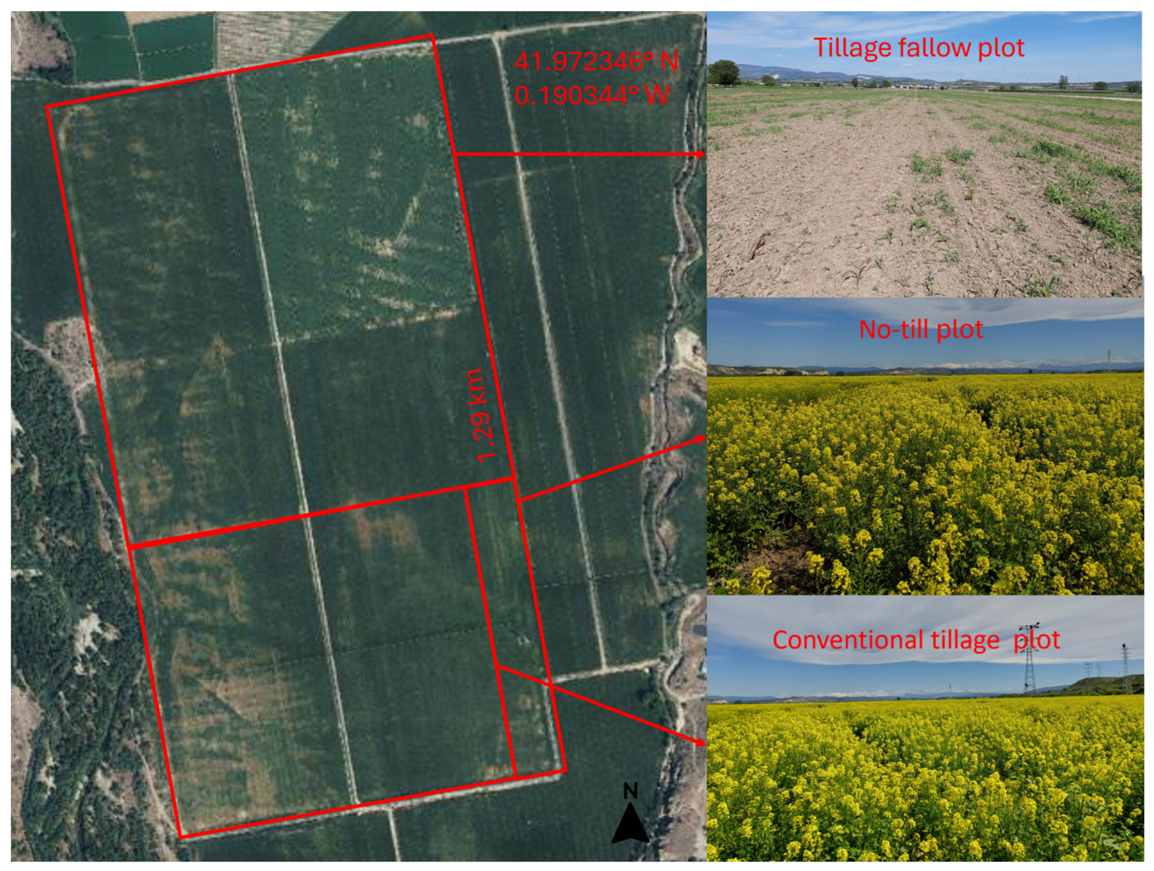
The experiment was conducted under field conditions in a 114 ha agricultural plot placed on the lower terrace of the Cinca River, on a Calcaric Fluvisol [22]. This field has traditionally been used for cultivating isogenic maize (Zea mays L.) for human consumption. However, in 2022, white mustard (Sinapis alba L.) was also sown as an intermediate cover crop at a seeding rate of 5 kg/ha. The total time period of the experiment corresponds to one full agricultural year. Maize, the main crop, was sown between April and May and harvested in October. Instead of leaving the soil fallow during the post-harvest period (October to the following April), a short-cycle service crop (Sinapis alba L.) was introduced to cover the soil and avoid bare ground. This cover crop was managed during the fallow phase and harvested before the next maize cycle began. Therefore, the experiment spanned the full year, including both the main crop and the intermediate cover crop phase. For this study, after maize harvest, the field was divided into two subplots, where white mustard (cover crop, CC) was sown using different sowing practices: no tillage (NT) on 4 ha, conventional tillage (CT) on 32 ha, and a tilled fallow plot without cover crop as a control (TF) on 78 ha. All plots were irrigated by a sprinkler, using a pivot irrigation system (Figure 1).
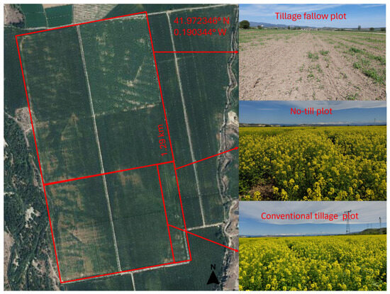
Figure 1.
Location of the treatments: tillage fallow plot (TF), no-till plot (NT), and conventional tillage plot (CT). Images of each treatment (right) correspond to the sampling conducted 90 days after sowing (DAS).
All plots received a basal fertilization of 20,000 L/ha of “enriched water,” a mixture consisting of water combined with cleaning residues from a fertilizer plant’s pipelines and by-products from the cogeneration of pig slurry. The exact chemical composition of this amendment is not fully characterized, as it is a complex mixture derived from industrial residues and organic by-products. This amendment is a routine practice applied by the landowner as a basal fertilizer. Importantly, this fertilization treatment was applied uniformly across the entire experimental area and to all treatments, ensuring that any effects observed are not confounded by differences in basal fertilization.
A metaldehyde-based phytosanitary treatment was applied after sowing.
2.2. Soil Sampling
To ensure representative sampling, each plot (TF, NT, and CT) was subdivided into four subplots, each 50 m wide (corresponding to the width between the wheels of the irrigation ranger), with variable lengths depending on the total area of each plot.
To assess the temporal variation in soil quality, sampling was carried out at 60 days after sowing (DAS) of the CC, and again at 90 DAS, corresponding to its peak development stage. During each sampling period, soil samples were collected from the 0–20 cm depth in all subplots, using a soil hand auger (Eijkelkamp). Each composite sample was formed by mixing 10 subsamples taken at 100 m intervals, resulting in four composite samples per treatment. In addition, to evaluate the effect of the cover crop on the surface soil layer, 10 undisturbed surface samples (0–6 cm) were randomly collected in each plot using a metal cylinder. The sampling depths were selected based on the criteria proposed by Duval et al. (2016) [23]. The sampling design was based on established criteria for soil studies in large-scale agricultural plots and was further supported by the relatively homogeneous conditions of the study site. The subplots are located on an alluvial terrace with uniform topography, which minimizes small-scale soil variability. The slope within the NT plot was 1.47 ± 1.11°, in the CT plot 1.77 ± 4.01°, and in the TF plot 1.68 ± 3.38°. Elevation values were also relatively consistent across treatments, with 271.09 ± 0.40 m in NT, 270.05 ± 0.93 m in CT, and 273.26 ± 1.23 m in TF.
2.3. Samples Processing and Determination of Soil Properties
Soil samples from the 0–20 cm depth were sieved through a 2 mm mesh and stored at 4 °C until analysis. Undisturbed samples from the 0–6 cm layer were used for mesofauna extraction (Berlese–Tullgren funnels) and for bulk density determination. Table 1 summarizes the physical, chemical, and biological indicators assessed in this study, along with the analytical protocols used.

Table 1.
Protocol measurements for indicators selected in the study.
Soil organic matter was estimated from carbon content using the Van Bemmelen factor [32].
Additionally, based on mesofauna quantification, the following biodiversity indices were calculated: Shannon–Wiener diversity index (H′), species richness (S), and Pielou’s evenness index (J′).
where S is the total number of species; and is the proportion of individuals belonging to species i, i.e., the number of individuals of species i divided by the total number of individuals in the community [32].
where H is the Shannon diversity index, and S is the number of species [32].
2.4. Soil Quality Evaluation Method
Given that soil is a complex ecosystem where multiple factors interact, its quality cannot be assessed using a single indicator [33]. Physical, chemical, and biological properties, along with the processes occurring in the soil, serve as indicators of its condition, functionality, and capacity to respond to changes in management. However, these indicators may vary depending on soil type and use, ecological function, pedogenetic factors, and climatic conditions, making it difficult to establish universal criteria for soil quality assessment [34].
The most used approaches for selecting indicators are the Total Data Set (TDS) and the Minimum Data Set (MDS) [35,36]. Several studies have shown that the MDS method is more suitable due to its efficiency and accuracy, as well as being faster and simpler to implement [36]. For this reason, the MDS approach was adopted in the present study. Once the appropriate indicators were selected, they were quantified and weighted to estimate the Soil Quality Index (SQI), following the equation developed by Andrews et al. (2004) [37]:
where is the weighted soil quality index for a given ecosystem, is the weighting factor for indicator i, is the score of the indicator, and is the number of indicators evaluated.
To evaluate the relationship between the indicators and soil quality, scoring functions were developed and classified into three types, S-shaped, inverse S-shaped, and parabolic (Table 2), depending on the influence of each indicator on soil quality. In these equations, represents the indicator value; is its score, which ranges between 0.1 and 1; and a and b correspond to the lower and upper thresholds, respectively. Threshold values for indicators with a strong agricultural relevance were established according to the methods used in the analytical determinations (Table 1). For the remaining parameters, reference values were taken from previous studies (Table 2).
Table 2.
Standard scoring functions and parameters for soil indicators.
The Ecological–Morphological Index (EMI) has been used as a biological index to evaluate soil mesofauna. This index is based on the classification of extracted specimens at the order or class level, assigning them a value between 1 (no soil adaptation) and 20 (maximum soil adaptation) [43,44]. Unlike other parameters, the EMI does not evaluate a specific soil function; rather, its relevance lies in the presence or absence of certain orders. Nonetheless, it was included in the SQI determination as an indicator.
To identify key indicators and establish the Minimum Data Set (MDS), a Principal Component Analysis (PCA) with normalized values was performed. In this analysis, each variable received a factor loading indicating its contribution to the total variance, with only those exhibiting high loadings being considered. When several variables were selected within the same principal component, multivariate correlation coefficients were calculated [34,35,37]. If two or more parameters showed significant correlation (r > 0.60, p < 0.05), the variable with the highest factor loading was retained to avoid redundancy [45].
To assess the evolution of soil quality, analytical results from samples collected at two sampling dates after the cover crop sowing and at two depths were analyzed. From these data, an SQI was calculated for each time x depth combination, yielding a total of four values: 60 DAS at depths of 0–6 cm and 0–20 cm, and 90 DAS at the same depths. Once calculated, the SQI value was interpreted as a direct measure of the suitability of the cover crop for agricultural use, with higher values indicating better soil quality [46,47].
2.5. Statistical Analysis
To evaluate the effect of the cover crop sowing method (NT, CT, and TF) and its temporal evolution, a two-way analysis of variance (ANOVA) was performed separately for each soil depth (0–6 cm and 0–20 cm) and the interaction among the two factors (sowing method x days after sowing). The pairwise comparison of Tukey’s HSD test (p < 0.05) was also used to evaluate the statistical significance of the differences in the response variables. When the data did not meet the assumptions of normality, even after transformation, a non-parametric Kruskal–Wallis test was conducted to assess the differences among groups. When significant differences were detected, Dunn’s post hoc test was applied for pairwise comparisons (p < 0.05). Pearson’s correlation coefficient was employed to analyze linear relationships, and Principal Component Analysis (PCA) was conducted to identify multivariate data patterns. All analyses were carried out using Past v.4.03 [48] and XLSTAT v.2024.2.2.1422 [49].
3. Results and Discussion
3.1. Effect of the Cover Crop on Soil Physical, Chemical, and Biological Properties
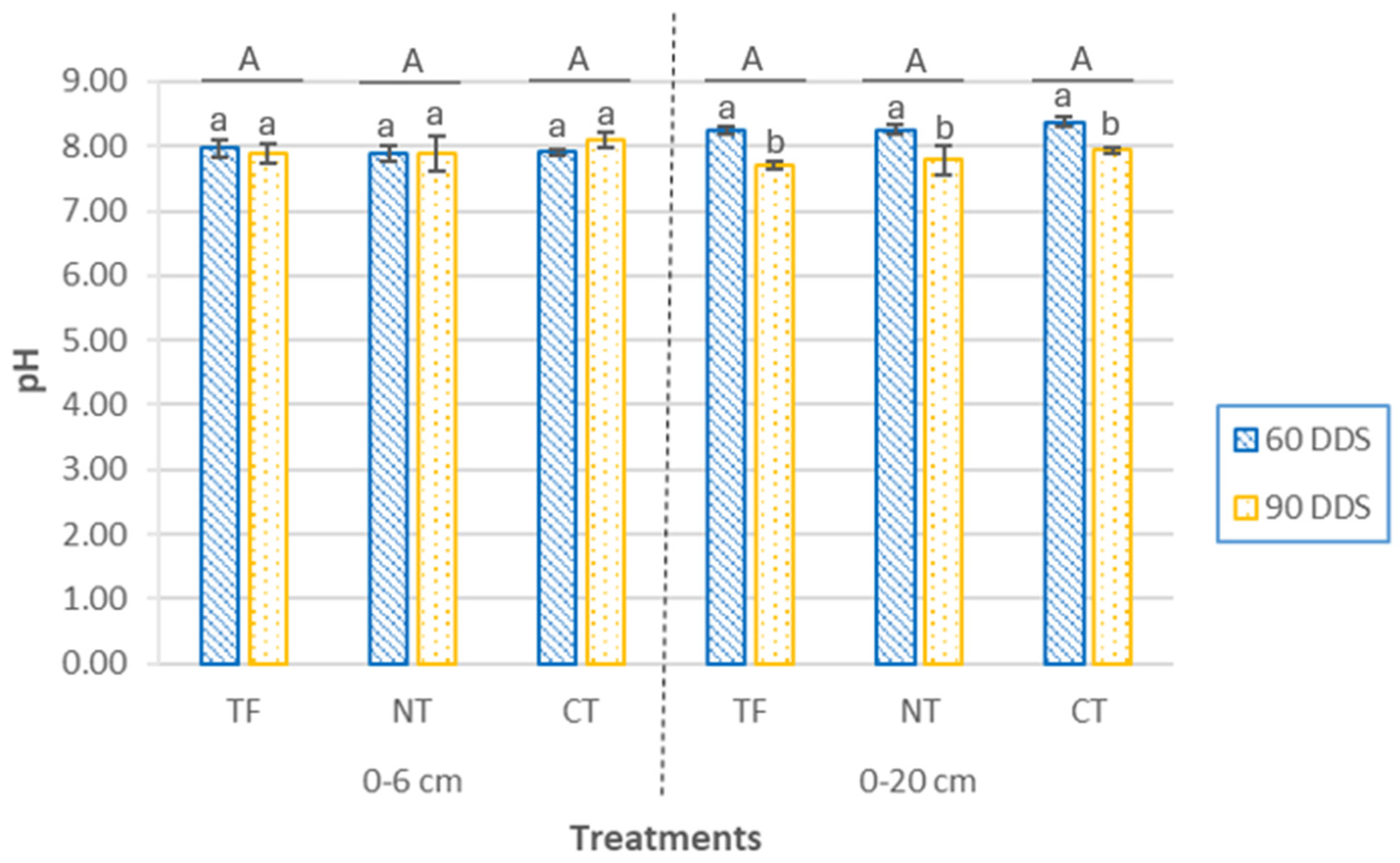
Overall, soil pH (Figure 2) was, on average, 0.5 units higher at the 0–20 cm depth compared to the 0–6 cm layer. At the surface (0–6 cm), pH values ranged from 7.88 ± 0.12 (NT, 60 DAS) to 8.11 ± 0.12 (CT, 90 DAS), characteristic of a basic soil with high availability of Ca2+ and Mg2+, but with limitations in phosphorus and micronutrient availability [39]. At this depth, no significant differences were observed between cover crop sowing treatments (p = 0.31). When comparing the two sampling times within each treatment, no significant differences were found between sampling periods within treatments (p = 0.57).
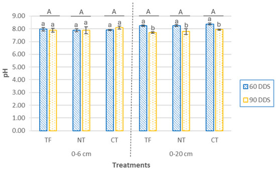
Figure 2.
pH values at two depths (0–6 cm and 0–20 cm) and two sampling times (60 DAS and 90 DAS), according to cover crop sowing treatments (TF, tillage fallow; NT, no till; and CT, conventional tillage). Lowercase letters indicate significant differences (p ≤ 0.05) between sampling periods within each treatment, while uppercase letters denote significant differences (p ≤ 0.05) between treatments. Bars represent the mean (n = 4) ± standard deviation.
At 0–20 cm depth, pH values ranged from 7.71 ± 0.07 (TF, 90 DAS) to 8.38 ± 0.07 (CT, 60 DAS), with no significant differences among treatments (p = 0.28). Nonetheless, when comparing sampling dates within each treatment, significant differences were detected (p < 0.001), with mean pH values significantly lower at 90 DAS. The significant pH decrease observed at 0–20 cm depth across all treatments between 60 and 90 days after sowing (DAS) likely reflects enhanced biological activity linked to root development and the decomposition of maize residues. These processes, including root exudation, microbial respiration, and organic acid production, can transiently acidify the rhizosphere, although such effects may be moderated over time by the buffering capacity of calcareous soils. These results are in line with previous studies reporting that tillage does not directly determine soil pH, but rather modulates biogeochemical processes whose effects depend on factors such as soil type, climate, and residue management [50].
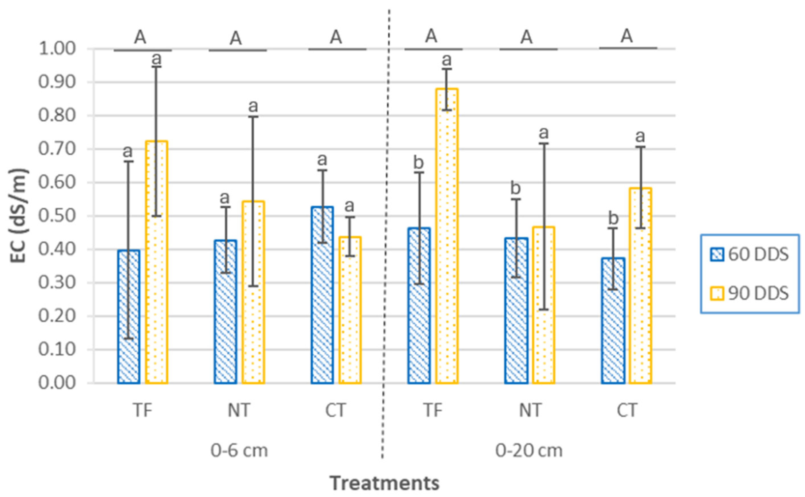
The electrical conductivity (EC) values across all plots, at both analyzed soil depths and during both sampling periods, ranged from 0.37 to 1.12 dS/m, as a result of seasonal variations in the concentration of ions solution (Figure 3). In the surface layer (0–6 cm), no significant differences were observed either between treatments (p = 0.61) or between sampling periods (p = 0.27). At the 0–20 cm depth, however, EC showed significant differences between the two sampling periods (p < 0.001), with a marked increase in EC observed at 90 days after sowing (DAS) across all treatments.

Figure 3.
EC values at two depths (0–6 cm and 0–20 cm) and two sampling times (60 DAS and 90 DAS) according to cover crop sowing treatments (TF, tillage fallow; NT, no till; and CT, conventional tillage). Lowercase letters indicate significant differences (p ≤ 0.05) between sampling periods within each treatment, while uppercase letters denote significant differences (p ≤ 0.05) between treatments. Bars represent the mean (n = 4) ± standard deviation.
The significant increase in EC observed at 90 DAS in the 0–20 cm soil layer may be explained, at least in part, by the accumulation of dissolved organic matter (DOM) in the soil solution. A strong and significant positive correlation was found between EC and DOM content (r = 0.80; p < 0.0001), indicating that higher levels of organic solutes likely contributed to increased ionic strength and, consequently, to higher EC values. This relationship suggests that the decomposition of organic residues and the associated release of soluble ions may play a key role in modulating soil salinity dynamics at this depth. As microbial activity intensifies during the cover crop growing period, particularly under warm conditions (spring), the decomposition of organic residues leads to the release of soluble ions and low-molecular-weight organic compounds that contribute to increased EC in the soil solution. This process is further enhanced by the upward or downward movement of water through the soil profile, which can redistribute soluble components and lead to their accumulation at intermediate depths. Previous studies have reported similar patterns, where increased DOM concentrations were associated with elevated EC values, highlighting the role of organic matter mineralization in modulating soil salinity [51].
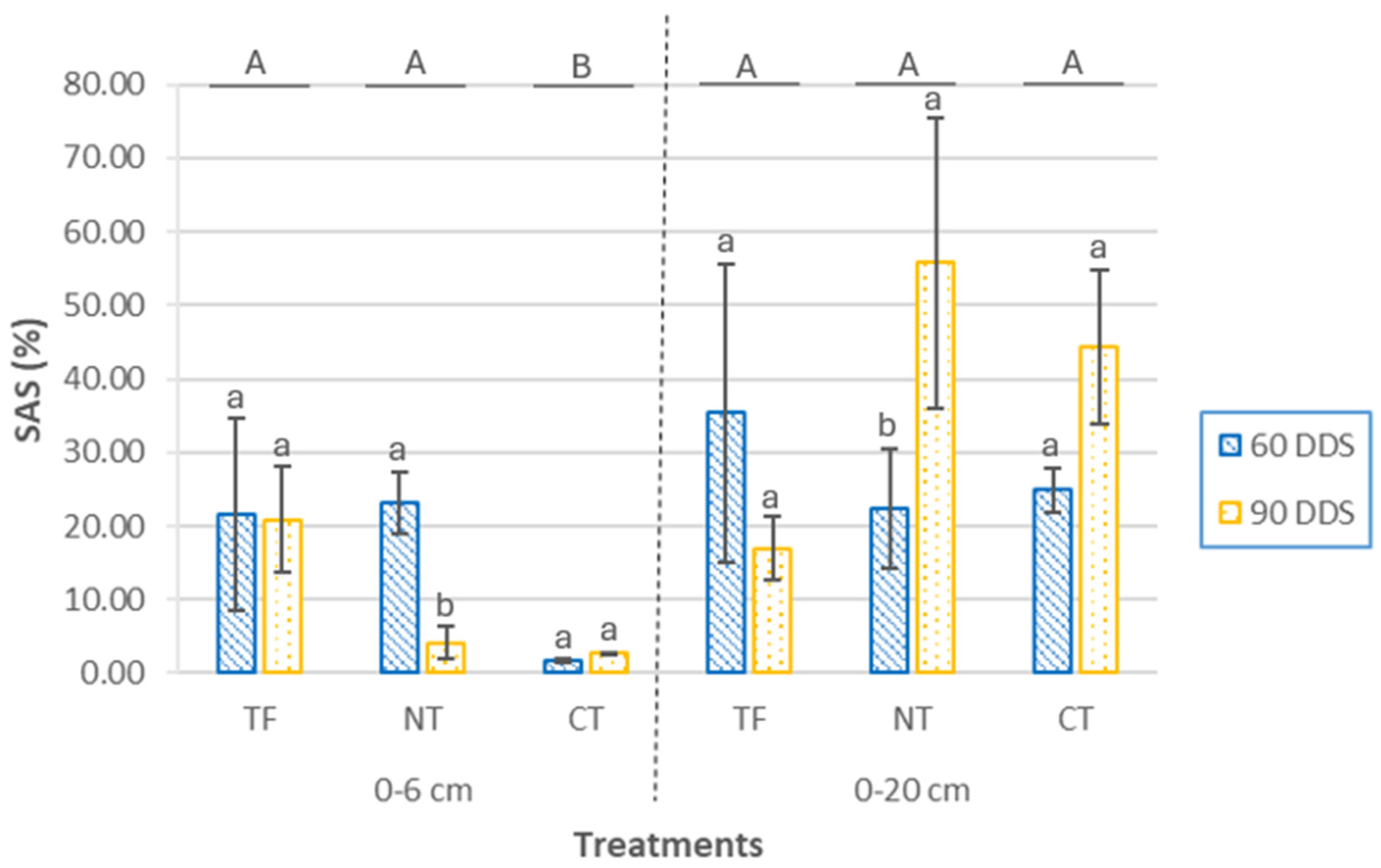
The structural stability values obtained are characteristic of surface horizons of cultivated soils, which typically exhibit low organic matter levels and are exposed to tillage with heavy machinery [4,52]. At the 0–6 cm depth (Figure 4), significant differences in soil aggregate stability (SAS) were observed among cover crop (CC) treatments (p < 0.001), with the conventional tillage (CT) treatment showing the lowest mean values. No significant differences were found between sampling times (p = 0.22), but there was a significant interaction effect (p = 0.014). This interaction was due to significant temporal differences only within the no tillage (NT) treatment (p = 0.043), where SAS was higher at 90 days after sowing (DAS).
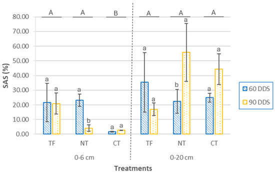
Figure 4.
Soil aggregate stability (SAS) at two depths (0–6 cm and 0–20 cm) and two sampling times (60 DAS and 90 DAS), according to cover crop sowing treatments (TF, tillage fallow; NT, no till; and CT, conventional tillage). Lowercase letters indicate significant differences (p ≤ 0.05) between sampling periods within each treatment, while uppercase letters denote significant differences (p ≤ 0.05) between treatments. Bars represent the mean (n = 4) ± standard deviation.
At 0–20 cm depth, SAS values ranged from 55.78 ± 19.70% (NT, 90 DAS) to 16.92 ± 4.34% (CT, 90 DAS), and were generally higher than those observed at the surface. No significant differences were found between treatments (p = 0.35) or sampling times (p = 0.050), but a significant interaction was detected (p = 0.026). As at the surface, the only significant difference was observed within the NT treatment between the two sampling times (p = 0.042). Structural stability was greater at the surface (0–6 cm) at 60 DAS, whereas in the subsurface layer (0–20 cm), higher values were recorded at 90 DAS. These results suggest a differential temporal development of soil structure under no-tillage management.
The results demonstrate that SAS is influenced by both agronomic practices (sowing method) and soil depth [53], with higher values observed at 0–20 cm. This suggests that subsurface layers are more responsive to management-induced changes. At 90 DAS, SAS increased notably in NT and CT treatments at this depth, likely reflecting the beneficial effects of cover crop development. Similar short-term improvements in structural stability under no-till systems with cover crops have been associated with increases in labile carbon pools [53]. Evidence from semi-arid regions also supports this pattern, with improvements in SAS in the 10–20 cm layer linked to higher levels of soil organic carbon and nitrogen [54]. Conservation practices—especially the combination of no-till system and cover cropping—have been shown to promote aggregate stabilization even under irrigated conditions [55]. In particular, the use of Sinapis alba L. as a winter cover crop has been associated with enhanced soil aggregate stability and porosity under reduced tillage, driven by increased root development and biological activity [56].
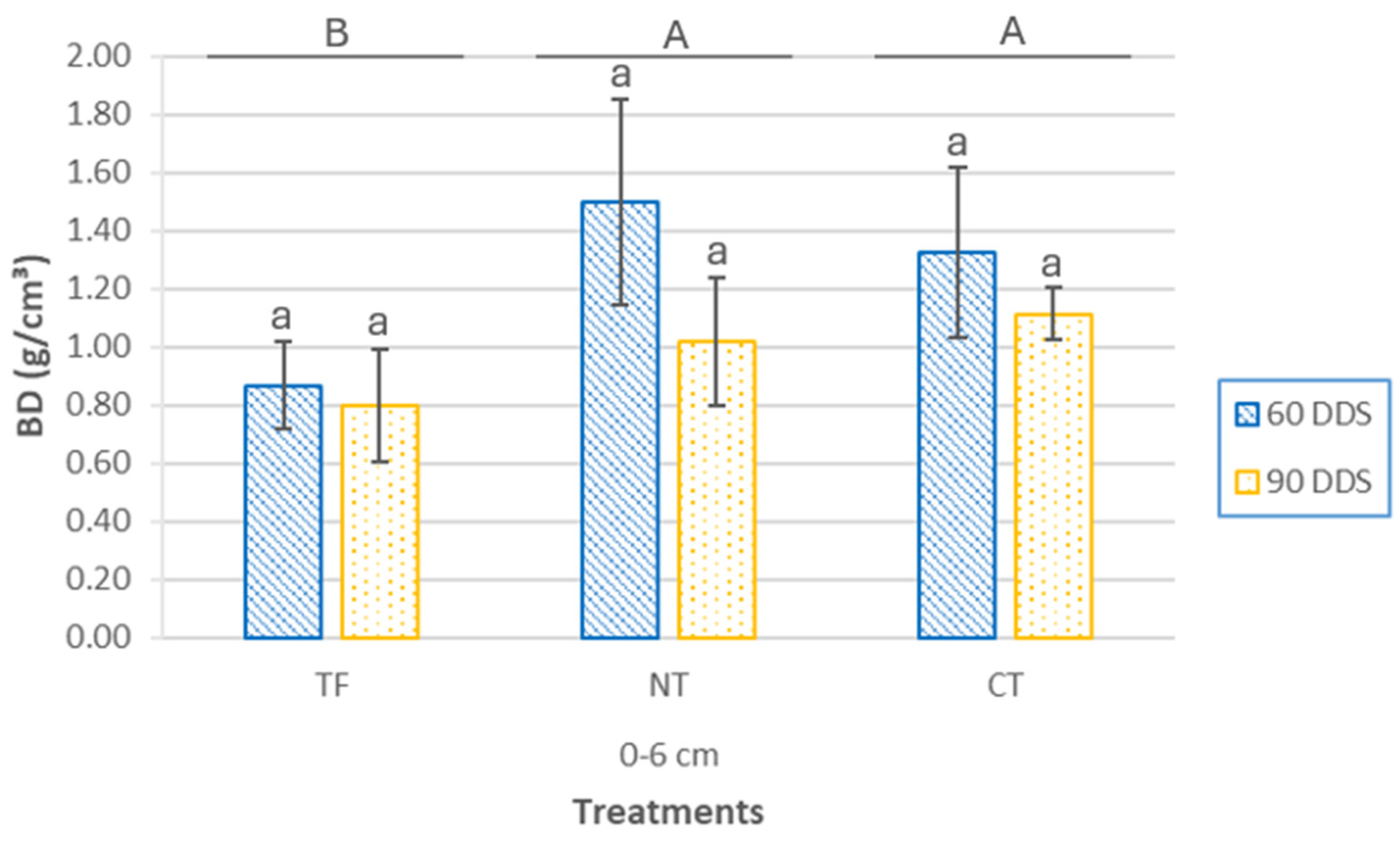
The CC sowing method significantly influenced soil bulk density (BD) values in the plots (Figure 5). Significant differences were observed among the CC sowing treatments (p = 0.003), with BD values similar for the NT and CT treatments, both significantly higher than the TF treatment. When analyzing the sampling dates within each treatment, no significant differences were found for TF (p = 0.58) or CT (p = 0.34). However, NT showed marginally significant differences (p = 0.061), with an average BD value 47% higher at 60 DAS compared to 90 DAS.
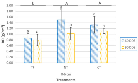
Figure 5.
Bulk density (BD) at surface (0–6 cm depth) and two sampling times (60 DAS and 90 DAS), according to cover crop sowing treatments (TF, tillage fallow; NT, no till; and CT, conventional tillage). Lowercase letters indicate significant differences (p ≤ 0.05) between sampling periods within each treatment, while uppercase letters denote significant differences (p ≤ 0.05) between treatments. Bars represent the mean (n = 4) ± standard deviation.
Although differences between sampling periods were not statistically significant—possibly because detecting changes in physical indicators generally requires more than four years of continuous CC growth [56]. BD values in the CT and NT treatments showed a reduction of 15% to 30% at 90 DAS. This suggests a progressive improvement in soil physical properties due to the cumulative effects of cover crop development. This trend is particularly relevant given the silty loam texture of the soil, which is naturally prone to compaction under conventional tillage. This improvement is partially driven by physical and biological processes associated with root growth, promoting soil loosening [57]. Conversely, the TF treatment consistently exhibited lower BD values compared to the other treatments. This pattern may be attributed to the continued use of conventional tillage in the TF system, typically resulting in lower bulk density in surface soil layers. In contrast, the NT and CT treatments are in the early stages of transition toward conservation agriculture, where a temporary increase in bulk density is commonly observed during the initial years of implementation [58].
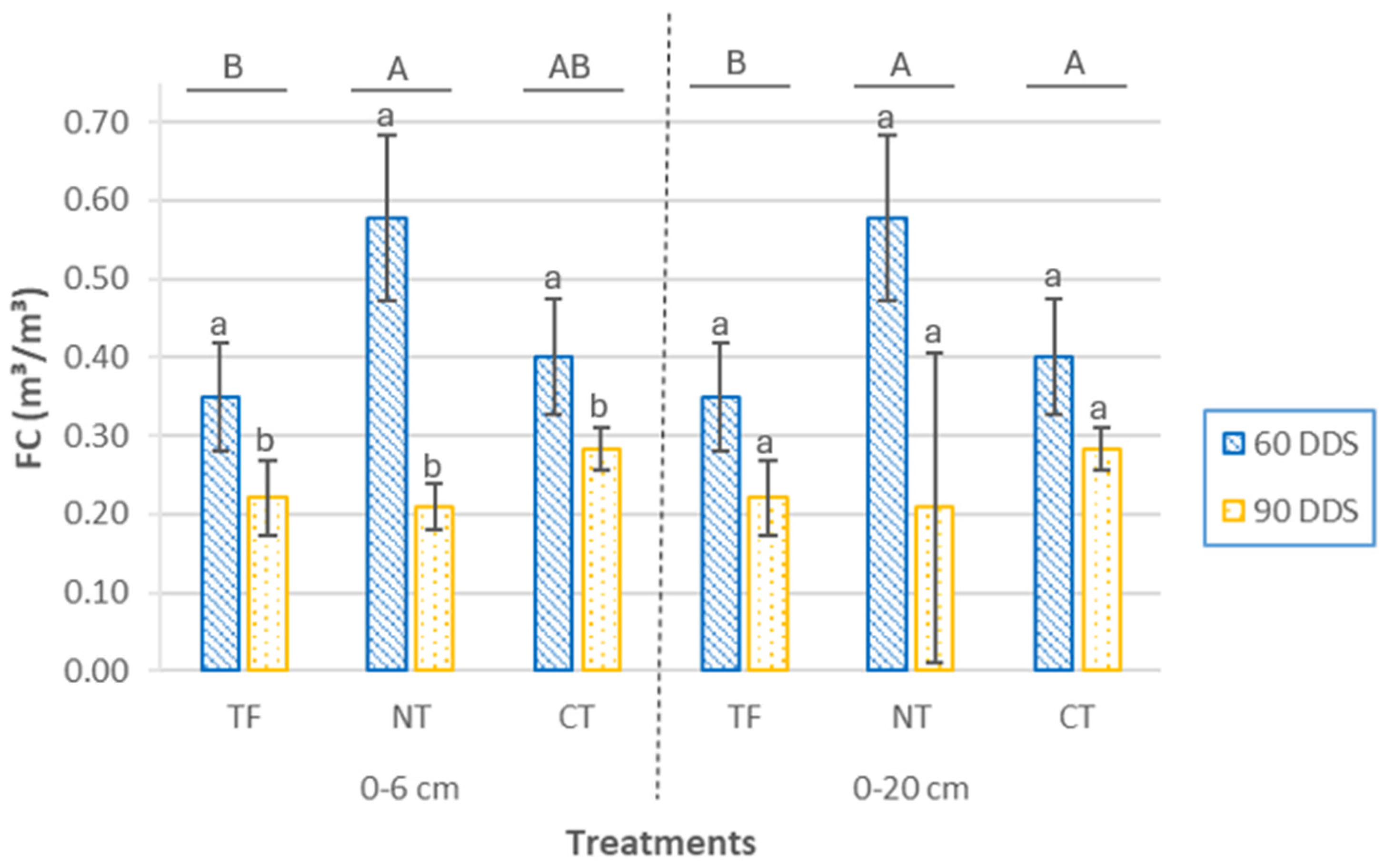
In the superficial layer, statistically significant differences were observed in the field capacity (FC) of the soil (Figure 6) between the sowing treatments (p = 0.003), with higher mean values in the NT and CT treatments, suggesting a greater water retention capacity, which benefits crop development under conditions of limited water availability [59]. At this depth, the sampling period had no statistically significant effect (p= 0.106) on FC values. At 0–20 cm soil depth, significant differences were observed among treatments (p= 0.012) and sampling periods (p < 0.001). The highest FC values were recorded in the NT treatment, followed by CT and, finally, TF, indicating a positive effect of reduced tillage intensity on soil water retention. In all plots, the mean FC value at 90 DAS was significantly lower than at 60 DAS, possibly due to porosity loss caused by soil settling after tillage. This behavior, common in short-term studies, may be more related to pre-sowing management practices, especially tillage, whereas the initial development of the cover crop—whose effect on soil structure and water retention requires more time to fully manifest—was still limited. This underscores the importance of the duration of management implementation to achieve substantial improvements in soil water dynamics [60,61].
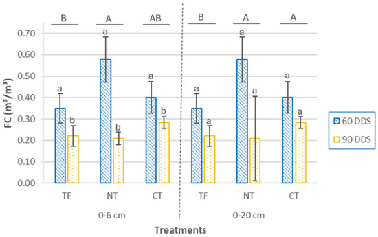
Figure 6.
Field capacity (FC) at two depths (0–6 cm and 0–20 cm) and two sampling times (60 DAS and 90 DAS), according to cover crop sowing treatments (TF, tillage fallow; NT, no till; and CT, conventional tillage). Lowercase letters indicate significant differences (p ≤ 0.05) between sampling periods within each treatment, while uppercase letters indicate significant differences (p ≤ 0.05) between treatments. Bars represent the mean (n = 4) ± standard deviation.
Soil organic matter (SOM) is a key indicator of soil quality due to its role in nutrient cycling, structural stability, and carbon sequestration. While cover crops (CCs) are widely recognized for enhancing SOM content, it is essential to distinguish between its different fractions, as their chemical nature determines both their stability and their function in the biogeochemical carbon cycle [62,63].
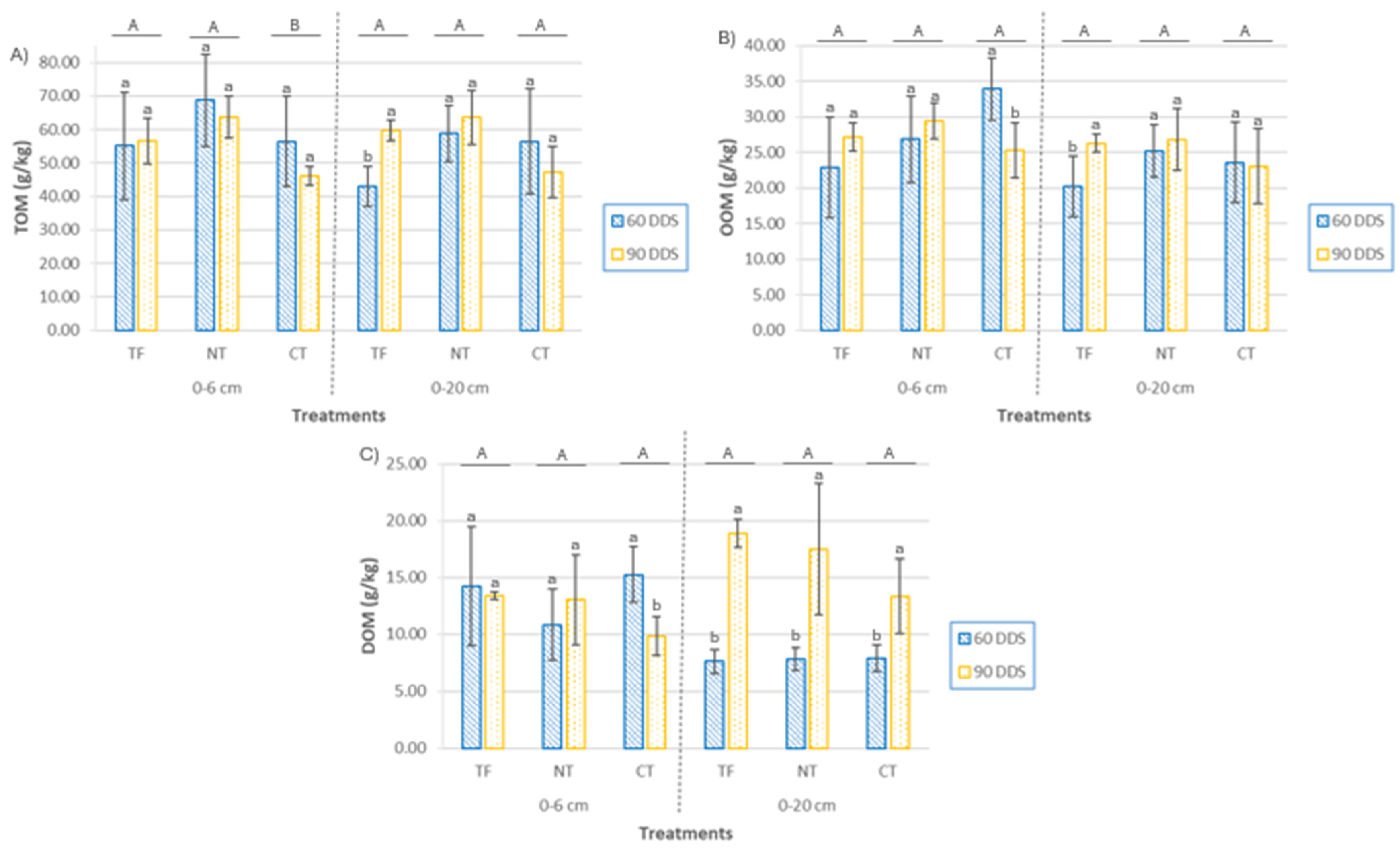
At the 0–6 cm depth, the sowing method significantly influenced total organic matter (TOM) content (Figure 7) (p = 0.039), with the highest values observed in the NT treatment, followed by the TF and CT treatments. However, no significant temporal variation was detected within treatments at this depth (p = 0.31). In contrast, at 0–20 cm, differences between treatments approached statistical significance (p = 0.057), and a significant decrease over time was observed in the TF treatment (p = 0.024), with lower TOM content at 60 DAS. Oxidizable organic matter (OxOM) content (Figure 7) ranged from 22.90 to 33.93 g/kg at 0–6 cm, and from 20.23 to 26.83 g/kg at 0–20 cm. Despite this variability, no statistically significant differences were found between treatments (p = 0.17 and p = 0.33) or sampling periods (p = 0.26 and p = 0.17), respectively. Dissolved organic matter (DOM) (Figure 7), recognized as a sensitive indicator of changes in soil biochemical status under varying management [34], did not differ significantly among treatments at either depth. However, a marked temporal increase in DOM was observed at 0–20 cm (p < 0.001), with concentrations at 90 DAS being 1.7 to 2.5 times higher than at 60 DAS across all treatments. This suggests an accumulation of soluble organic compounds, potentially linked to increased microbial activity and residue decomposition as the cover crop developed.
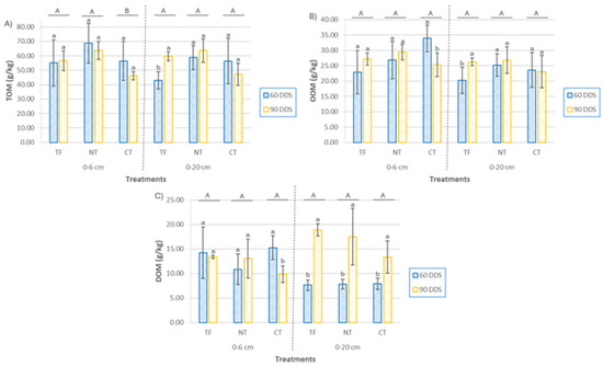
Figure 7.
(A) Total organic matter (TOM), (B) oxidizable organic matter (OxOM), and (C) dissolved organic matter (DOM) in soil at two depths (0–6 cm and 0–20 cm) at two sampling times (60 DAS and 90 DAS), according to cover crop (CC) sowing treatments (TF, tillage fallow; NT, no till; and CT, conventional tillage). Lowercase letters indicate significant differences (p ≤ 0.05) between the two sampling periods within each treatment, while uppercase letters indicate significant differences (p ≤ 0.05) between treatments. Each bar represents the mean (n = 4) and standard deviation.
Although short-term changes in SOM are often limited following the introduction of cover crops and shifts in tillage practices, an increase in TOM was detected at the surface in NT plots. This accumulation is likely attributable to crop residues left on the soil surface after harvest, a typical feature of no-till systems [43,64,65]. Since TOM encompasses both labile and stable fractions, this increase may reflect transient contributions from partially decomposed residues. In contrast, tilled plots displayed lower surface residue cover (10–20%) [43], reducing such accumulation. With increasing depth, treatment differences diminished, but SOM in TF plots tended to be lower, likely due to early-stage residue decomposition and delayed stabilization. The OxOM fraction remained unchanged across treatments and sampling times, underscoring its limited responsiveness over short time scales [62,63]. By contrast, DOM content significantly increased at 0–20 cm depth by 90 DAS in all treatments. This rise likely resulted from intensified microbial activity and vertical mobilization of labile organic compounds. The increase in DOM was strongly and negatively correlated with soil pH (r = −0.834, p < 0.001), suggesting that acidification promotes solubilization of organic matter and stimulates biogeochemical processes [30,62,66]. These dynamics may influence the vertical distribution of the soil C/N ratio. Specifically, surface accumulation of high-C/N residues in NT may temporarily elevate the C/N ratio due to nitrogen immobilization, while the concurrent increase in DOM and lower pH at depth could facilitate microbial turnover and release of low-C/N compounds, thereby reducing the C/N ratio in subsurface layers [67]. The SOM balance between 60 and 90 DAS supports these dynamics: at the surface (0–6 cm), the control treatment exhibited increases in all fractions; CT showed consistent declines; and in NT, TOM decreased slightly, while OxOM and DOM increased. At 0–20 cm depth, all treatments showed positive balances across fractions except for TOM in CT, which continued to decline. Notably, DOM rose sharply in both the control (+152.79%) and NT (+126.75%) treatments, indicating a substantial mobilization of labile organic matter under reduced tillage.
Various studies have highlighted the potential of soil proteins extracted using citrate and autoclaving (ACE proteins), commonly referred to as Glomalin-Related Soil Proteins (GRSPs), as sensitive bioindicators of soil health. Traditionally associated with arbuscular mycorrhizal fungi, recent research suggests that these proteins may represent a broader class of compounds more closely related to humic substances than to pure fungal glycoproteins [68]. This evolving understanding helps explain the strong correlations between GRSP and key soil properties, such as organic matter content, aggregate stability, and nitrogen reserves. Their relatively low seasonal variability and responsiveness to management practices, such as tillage, cover cropping, and crop rotation, further support their utility as indicators of agroecological sustainability. Their chemical nature remains under debate, but GRSPs are known to contribute to soil aggregation and structural stability due to their hydrophobic character and affinity for soil particles, ultimately helping to reduce erosion. For all of these reasons, their inclusion in SQI can provide complementary insights into soil fertility, physical stability, and resilience to disturbance.
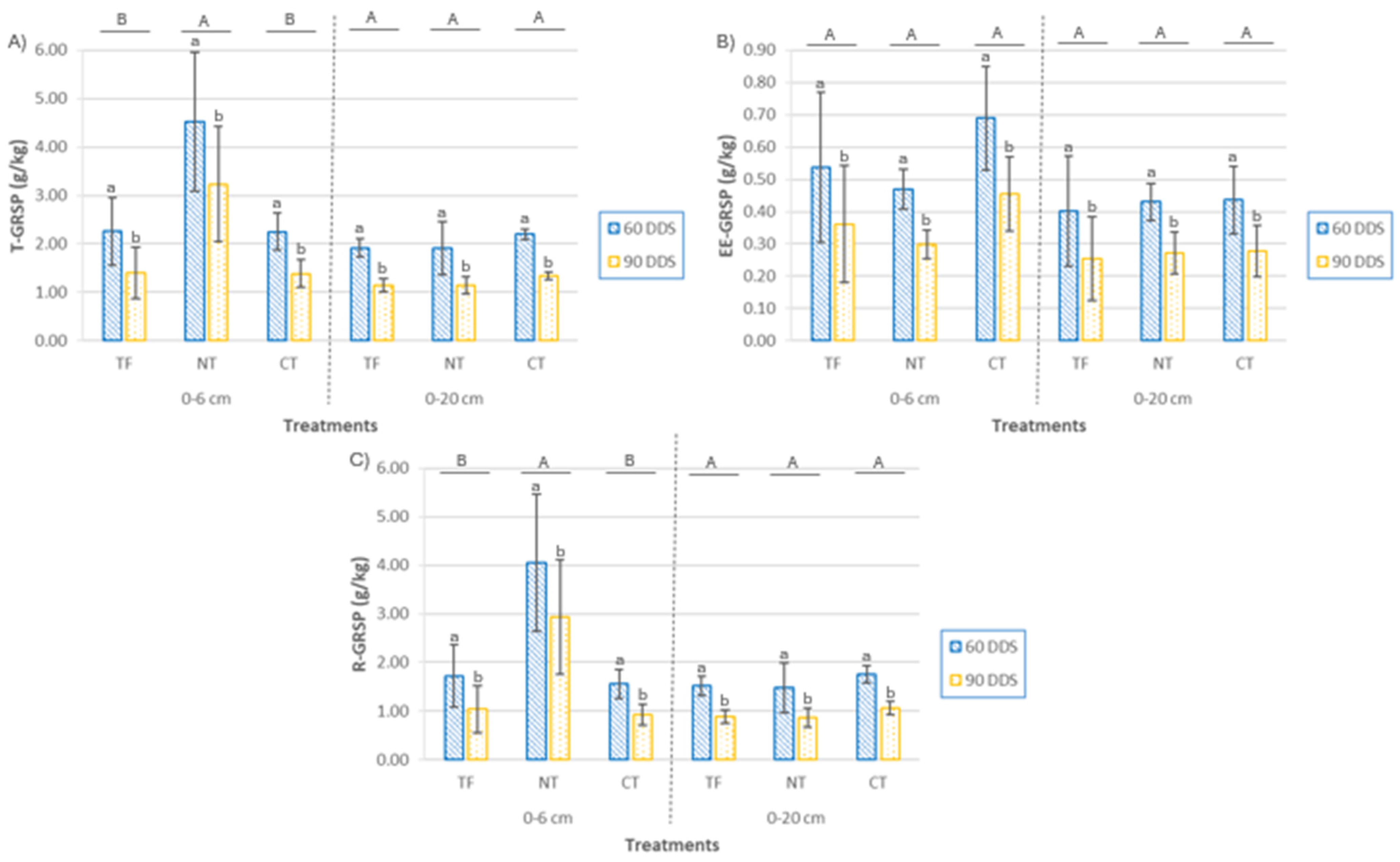
The glomalin fractions showed distinct responses to CC sowing and sampling time (Figure 8). Total glomalin (T-GRSP) concentrations at 0–6 cm depth were significantly higher under NT, approximately double those in CT and FT treatments (p < 0.001). In contrast, the easily extractable fraction (EE-GRSP) did not differ significantly between treatments at either 0–6 cm (p = 0.058) or 0–20 cm depth (p = 0.079). Sampling time had a significant effect on both fractions across depths. T-GRSP concentrations declined markedly from 60 to 90 days after sowing (DAS), with reductions of 29% to 39% at the surface (p = 0.01) and 38.4% to 41.0% at 0–20 cm depth (p < 0.001). Similarly, EE-GRSP decreased by an average of 52% at 0–6 cm (p = 0.005) and 33% at 0–20 cm (p = 0.013). EE-GRSP was consistently more abundant in surface soils, with mean values 35.5% higher than deeper layers at 60 DAS and 17% higher at 90 DAS. The EE-GRSP/T-GRSP ratio, an indicator of carbon stabilization associated with glomalin [69], showed significant treatment differences at the soil surface (p = 0.0013). NT plots had the lowest ratio, with EE-GRSP comprising only 17% of total GRSP, compared to 24–30% in tilled treatments. This suggests enhanced transformation of labile glomalin into more stable forms under NT management. No significant differences were detected at 0–20 cm depth (p = 0.22), and sampling time did not significantly affect this ratio at either depth. These vertical and compositional patterns highlight the contrasting behaviors of glomalin fractions: T-GRSP appears more stable and linked to long-term carbon accumulation, whereas EE-GRSP is more dynamic and responsive to short-term environmental and management changes.
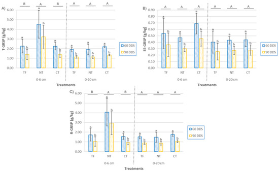
Figure 8.
(A) total glomalin content (T-GRSP), (B) easily extractable glomalin (EE-GRSP; panel (B)), and (C) recalcitrant glomalin (R-GRSP) in soil at two depths (0–6 cm and 0–20 cm) and two sampling times (60 and 90 DAS), according to cover crop planting treatments (TF, tillage fallow; NT, no till; and CT, conventional tillage). Lowercase letters indicate significant differences (p ≤ 0.05) between sampling times for each treatment, and uppercase letters indicate significant differences (p ≤ 0.05) among treatments. Each bar represents the mean (n = 4) and standard deviation.
Glomalin-type proteins’ sensitivity to agricultural practices supports their role as valuable indicators of soil health and agroecological sustainability. In this study, T-GRSP at the soil surface correlated positively and significantly with total organic matter (TOM) (r = 0.524, p = 0.009), aligning with previous findings that link glomalin content with organic carbon levels in agricultural soils [68,69,70].
EE-GRSP, representing the more labile glomalin fraction and recent microbial production, was significantly more abundant in surface layers. While the taproot system of mustard might limit microbial stimulation near the surface, lower GRSP concentrations were not observed there, suggesting that other factors, like legacy effects of previous crops and glomalin stabilization within the soil matrix, help maintain surface levels across depths [69]. Recalcitrant glomalin (R-GRSP) accumulated more in NT plots’ surface soils, likely reflecting enhanced persistence and physical protection against microbial degradation in reduced disturbance systems [70]. Evaluating the T-GRSP/TOM ratio revealed significant differences between NT and tilled treatments, reinforcing the impact of soil management on glomalin dynamics. The higher ratio at the surface under NT (~5% of soil organic matter pool) suggests improved glomalin preservation, while lower ratios in tilled plots indicate disruption of glomalin accumulation despite cover crop presence. At deeper layers (0–20 cm), the opposite trend suggests tillage may facilitate glomalin incorporation into subsoil horizons [71]. This complex spatial distribution indicates trade-offs in soil carbon sequestration between conservation and tillage practices. Temporal changes strongly influenced glomalin parameters. All treatments showed a marked decline in T-GRSP, EE-GRSP, and the T-GRSP/TOM ratio from 60 to 90 DAS, across depths. This may relate to the introduction of Sinapis alba, a non-mycorrhizal cover crop species, which likely reduces symbiotic interactions and, thus, glomalin production [71]. Additionally, microbial degradation transforms labile EE-GRSP into more recalcitrant forms, contributing to this decline. Interestingly, contrary to several studies reporting positive correlations between EE-GRSP and soil aggregate stability (SAS), this study found a significant negative correlation at 0–20 cm (r = −0.715, p < 0.001). This suggests that higher EE-GRSP concentrations do not always translate into enhanced aggregate stability, potentially due to accumulation in structurally inactive forms. Standard extraction protocols for GRSP may retrieve fractions not contributing to physical soil stabilization, a factor particularly relevant in conventionally tilled soils where oxidation and mechanical disturbance could release non-bound glomalin [71]. Moreover, distinct temporal dynamics of EE-GRSP and SAS were evident: in NT plots, EE-GRSP slightly declined between 60 and 90 DAS, while SAS increased considerably, possibly reflecting glomalin’s initial role in aggregate formation followed by integration into more stable organic matter fractions [72]. Finally, it is important to consider that soil aggregate stability depends on multiple interacting factors, including organic matter, root activity, and microbial communities. The formation and stabilization of aggregates result from complex physical, chemical, and biological processes [73,74].
Considering the bioindicator function of soil mesofauna, no significant differences were observed in the biodiversity indices obtained across the different treatments (Table 3). The Shannon index showed a p-value of 0.94, species richness showed p = 0.38, and Pielou’s evenness index showed p = 0.77, indicating a homogeneous community structure regardless of the management applied. In all cases, the Shannon index reflects low diversity, with values ranging between 0.91 ± 1.41 and 1.67 ± 0.18. This range is below the normal values expected in natural ecosystems, where higher species diversity is typical [75].
Table 3.
Mesofauna diversity by species richness, the Shannon–Wiener index, and Pielou’s evenness index (n = 13). Means ± standard deviations are presented for each treatment, along with significance levels (p-values).
Although no significant differences were found among treatments, the mean values of the ecological indices were lower during the period of maximum CC development (90 DAS). This decrease can be associated with the increased dominance of the previously mentioned species at 90 DAS. However, despite the reduction in the mean Shannon index value at 90 DAS, the mean species richness remained practically constant throughout the CC growth period. Regarding evenness, measured by Pielou’s index, a decrease in mean values was observed across all treatments during the second sampling, consistent with the observed lower diversity.
In all the surface samples and treatments analyzed, the highest number of identified species corresponded to the groups Collembola and Acari. The ecological importance of both groups lies in their value as biological indicators. Several studies have highlighted the importance of Acari for assessing the nature of the ecosystem and the disturbances occurring within it [76,77]. Similarly, Collembola have been widely used as bioindicators of soil contamination, being sensitive to changes in pH, moisture, and organic matter content [78,79]. Due to this high sensitivity, both groups allow detection of differences between ecosystems with varying degrees of disturbance, so that an increase in the number of observed species highlights the positive role of white mustard as a CC on soil biodiversity.
A detailed analysis of the two dominant groups of identified soil mesofauna revealed shifts in suborder composition depending on the developmental stage of the cover crop (CC). At 60 DAS, mites were dominated by the suborders Cryptostigmata, primarily decomposers, and Uropodina, which are mainly predators. However, during peak CC development, a greater diversity of mite suborders was observed, with no single group dominating. For Collembola, the early growth stages of the CC were characterized by the predominance of individuals from the genera Tomocerina and Entomobrya. In contrast, at peak development, there was a higher presence of individuals from the order Poduromorpha, all of which are decomposers.
The presence and variation in these mite and springtail suborders suggest that the agroecosystem is influenced by factors such as organic matter, moisture, and agricultural practices. Nevertheless, despite the potential of these organisms as bioindicators, they cannot yet be considered key indicators due to the lack of knowledge about their ecology, biology, and physiology, making the information their study provides partial [79,80].
3.2. Soil Quality Index (SQI)
Once the Minimum Data Set (MDS) indicators were determined, their relative weights were calculated (Table 4) [45].
Table 4.
Relative weights of soil quality indicators according to the MDS for samples taken at 60 and 90 DAS, at depths of 0–6 cm and 0–20 cm.
An analysis of the normalized weights of the indicators included in the SQI reveals variations depending on both soil depth and sampling time. At 60 days after sowing (DDS), the surface layer (0–6 cm) was dominated by physicochemical indicators such as BD (0.40), EC (0.40), DOM (0.40), TOM (0.35), and OxOM (0.35), with notable contribution from the biological indicator EE-GRSP (0.40). These results reflect the greater sensitivity of the upper soil layer to management practices and early crop development stages.
In the 0–20 cm layer at the same time point, the highest weights were also associated with physicochemical indicators, including pH (0.43), EC (0.43), SAS (0.43), FC (0.38), TOM (0.38), and OxOM (0.38), suggesting a more stable environment, characterized by slower accumulation and transformation processes.
At 90 DDS, a redistribution of indicator weights was observed. In the 0–6 cm layer, pH, EC, and TOM exhibited the highest weights (each 0.47), indicating a transition toward more consolidated soil conditions. In contrast, the contribution of physical indicators such as SAS decreased notably (0.12). EE-GRSP was excluded from this stage, having been deemed redundant according to the MDS procedure, while T-GRSP showed an intermediate weight (0.26). In the 0–20 cm layer, pH (0.42), TOM (0.42), and FC (0.42) again stood out, reinforcing the trend toward the predominance of chemical indicators in the later stages of the cropping cycle.
The SQI, derived from the MDS indicators, is used to assess soil quality following the introduction of white mustard as a cover crop (Figure 9). The indices are calculated throughout the crop’s development (60 and 90 DAS) at both surface (0–6 cm) and subsurface (0–20 cm) layers. It is important to highlight that analysis of variance (ANOVA) is a key statistical tool in this type of study, as it allows for the objective identification of which parameters significantly influence soil quality at the agricultural scale. This approach provides quantitative support for the results obtained through the SQI. However, it should be noted that, in some cases, laboratory analyses may reveal significant differences between treatments that are not as clearly reflected in the SQI. This is because individual values may fall within ranges considered suitable for the agroecosystem under evaluation, thereby minimizing their impact within the composite index. Therefore, the SQI not only synthesizes complex information but also contextualizes it within a functionally and agronomically relevant framework.

Figure 9.
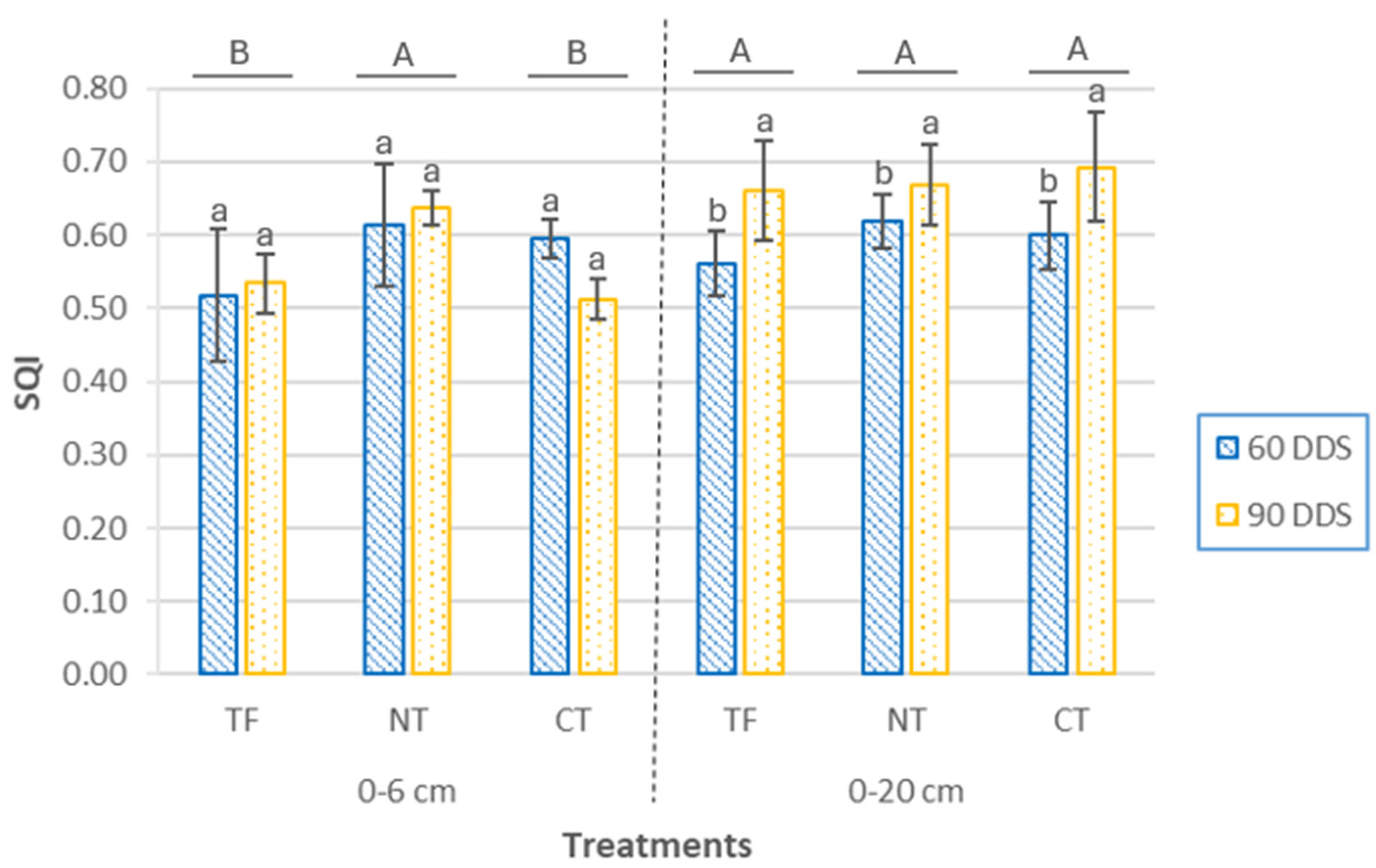
Soil Quality Index (SQI) at two depths (0–6 cm and 0–20 cm) and two sampling times (60 DAS and 90 DAS), according to cover crop sowing treatments (TF, tillage fallow; NT, no till; and CT, conventional tillage). Lowercase letters indicate significant differences (p ≤ 0.05) between sampling periods within each treatment, while uppercase letters indicate significant differences (p ≤ 0.05) between treatments. Bars represent the mean (n = 4) ± standard deviation.
At the 0–6 cm depth, the SQI showed significant differences between treatments (p = 0.00073), while no significant effects were detected for sampling time (p = 0.55) or the treatment × time interaction (p = 0.13). SQI values ranged from 0.51 ± 0.03 (CT, 90 DDS) to 0.64 ± 0.02 (NT, 90 DDS). At both sampling times, CT and TF treatments exhibited similar SQI values, whereas NT differed significantly, showing increases of 18.46% and 2.94% compared to TF and CT, respectively, at 60 DDS, and 19.17% and 24.31% at 90 DDS.
At the 0–20 cm depth, no significant differences were observed between treatments (p = 0.38) or for the interaction (p = 0.63), although sampling time had a significant effect (p = 0.0018). In all cases, SQI was higher at 90 DDS, indicating a positive effect of cover crop establishment. Values ranged from 0.56 ± 0.04 (TF, 60 DDS) to 0.69 ± 0.08 (CT, 90 DDS). Although differences among treatments were not statistically significant, at 60 DDS the NT treatment exhibited an SQI value 10.24% higher than TF and 3.05% higher than CT. These differences decreased at 90 DDS, suggesting a convergence in soil quality among treatments as the crop cycle progressed.
Regarding the relative ranking of treatments, at 60 DDS, the SQI order for both the 0–6 cm and 0–20 cm soil layers was TF < CT < NT. At 90 DDS, the pattern shifted slightly: in the surface layer, it was CT < TF < NT, and at depth, TF < NT < CT. This variability suggests that, while conservation practices exhibit more pronounced benefits in surface layers, soil responses at greater depths appear to be more influenced by slower accumulation processes and long-term management effects.
From a comparative perspective, NT was the only treatment to show consistent SQI increases across both depths and sampling times, particularly in the surface layer. In contrast, CT, despite achieving the highest value at depth at 90 DDS, showed a marked decline in surface quality. TF showed a positive trend in depth (+17.86%) but maintained low surface values. These patterns indicate that the benefits of conservation tillage not only emerge quickly in sensitive surface layers but may also extend to deeper layers as the management system matures.
According to established criteria for soil quality evaluation, this study classifies the SQI of maize plots with an intermediate mustard cover crop into five categories [46]: high (0.8–1), relatively high (0.6–0.8), moderate (0.4–0.6), relatively low (0.2–0.4), and low (0–0.2) [47]. Based on these thresholds, most SQI values in this study fall within the relatively high and moderate categories. The NT treatment was the only one to maintain relatively high SQI values at both studied soil depths and sampling times.
These findings suggest that while cover cropping can confer agronomic benefits, it is conservation tillage (NT) that has the most decisive impact on improving soil quality. In contrast, conventional tillage (CT) tends to degrade surface soil quality, accelerating degradation processes. Conservation practices not only enhance topsoil properties but also promote positive effects at depth, even during the early stages of cover crop establishment. These management approaches foster soil structure recovery, improve water retention, reduce profile temperature, and increase resistance to compaction [4]. Additionally, the accumulation of organic residues, such as maize stubble, alters nutrient dynamics, enhances rainfall infiltration, and acts as a thermal barrier, reducing evaporation [64]. These effects may explain the improvement observed under the fallow treatment (TF), which showed some gains at depth but failed to improve surface soil quality, indicating limited effectiveness in preserving upper soil functionality.
4. Conclusions
This study provides insights into how winter cover crops, particularly white mustard (Sinapis alba), interact with tillage to influence soil quality in intensive maize-based systems. The results partially support the initial hypothesis: introducing a short-cycle cover crop between main crop cycles can enhance soil quality, especially when combined with conservation practices like no tillage. Improvements in physical, chemical, and biological indicators contributed to significant increases in the Soil Quality Index (SQI).
However, the effects varied by soil depth. At 0–6 cm, the SQI showed differences between treatments but remained stable between 60 and 90 days after sowing (DAS), indicating that management practices strongly influenced soil properties in this surface layer. In some cases, physical, chemical, or biological properties even declined, likely due to the impact of tillage or other management actions, limiting the positive influence of the cover crop. Conversely, at 0–20 cm, where treatment effects were less pronounced, the SQI improved significantly over time, suggesting that the benefits of the cover crop became more evident at greater depths, less affected by surface management disturbances.
These findings highlight the importance of considering the depth of sampling soil when assessing the effects of cover crops and tillage on soil quality. They also emphasize the need for long-term studies and deeper soil sampling to better capture improvements associated with cover cropping and sustainable management practices.
Author Contributions
S.Q.-E. performed the analyses, statistical work, and wrote the original manuscript; C.M. performed the conceptualization and assisted with the methodology, statistics, and writing—original draft preparation writing; O.O. contributed to writing; D.B. performed funding acquisition, and writing—review and editing. All authors have read and agreed to the published version of the manuscript.
Funding
This research received no external funding.
Institutional Review Board Statement
Not applicable.
Informed Consent Statement
Not applicable.
Data Availability Statement
Data are contained within the article.
Acknowledgments
The authors would like to thank Elena Oyaga, agricultural engineer at Quality Corn Company, for kindly granting access to the sampling plots, making it possible to carry out this study.
Conflicts of Interest
The authors declare no conflicts of interest. The funders had no role in the design of the study; in the collection, analyses, or interpretation of data; in the writing of the manuscript; or in the decision to publish the results.
Abbreviations
The following abbreviations are used in this manuscript:
| CC | cover crops |
| CT | conventional tillage |
| NT | no tillage |
| TF | tillage fallow |
| DAS | days after sowing |
| SQI | Soil Quality Index |
| FC | field capacity |
| SAS | structural stability of aggregates |
| BD | bulk density |
| EC | electrical conductivity |
| TOM | total organic matter |
| OxOM | oxidizable organic matter |
| DOM | dissolved organic matter |
| T-GRSP | total glomalin fraction |
| EE-GRSP | extractable glomalin fraction |
| R-GRSP | recalcitrant glomalin fraction |
| H′ | Shannon–Wiener diversity index |
| S | species richness |
| J′ | Pielou’s evenness index |
| TDS | Total Data Set |
| MDS | Minimum Data Set |
| EMI | Ecological–Morphological Index |
| PCA | Principal Component Analysis |
| SOM | soil organic matter |
| GSRP | Glomalin-Related Soil Proteins |
References
- Adhikari, K.; Hartemink, A.E. Linking soils to ecosystem services—A global review. Geoderma 2016, 262, 101–111. [Google Scholar] [CrossRef]
- Wang, X.; Cheng, L.; Xiong, C.; Whalley, W.R.; Miller, A.J.; Rengel, Z.; Zhang, F.; Shen, J. Understanding plant–soil interactions underpin enhanced sustainability of crop production. Trends Plant Sci. 2024, 29, 1181–1190. [Google Scholar] [CrossRef] [PubMed]
- Jiang, P.; Wang, Y.; Zhang, Y.; Fei, J.; Rong, X.; Peng, J.; Yin, L.; Luo, G. Intercropping enhances maize growth and nutrient uptake by driving the link between rhizosphere metabolites and microbiomes. New Phytol. 2024, 243, 1506–1521. [Google Scholar] [CrossRef] [PubMed]
- Blanco-Canqui, H.; Ruis, S.J. No-tillage and soil physical environment. Geoderma 2018, 326, 164–200. [Google Scholar] [CrossRef]
- Comisión Europea. El Pacto Verde Europeo. Available online: https://ec.europa.eu/info/strategy/priorities-2019-2024/european-green-deal_es (accessed on 15 May 2025).
- Food and Agriculture Organization of the United Nations. Soils Are the Foundation for Vegetation; FAO: Rome, Italy, 2015; Available online: https://www.fao.org/fileadmin/user_upload/soils-2015/docs/Fact_sheets/En_IYS_Veg_Print.pdf (accessed on 15 May 2025).
- Doran, J.W.; Parkin, T.B. Defining and assessing soil quality. In Defining Soil Quality for a Sustainable Environment, 1st ed.; Doran, J.W., Jones, A.J., Eds.; SSSA: Madison, WI, USA, 1994; Volume 35, pp. 1–21. [Google Scholar] [CrossRef]
- Food and Agriculture Organization of the United Nations. El Estado Mundial de la Biodiversidad para la Alimentación y la Agricultura; FAO: Rome, Italy, 2019; Available online: https://www.fao.org/ (accessed on 15 May 2025).
- McDonald, H.; Frelih-Larsen, A.; Lóránt, A.; Duin, L.; Andersen, S.P.; Costa, G.; Bradley, H. Carbon Farming: Making Agriculture Fit for 2030; Policy Department for Economic, Scientific and Quality of Life Policies, European Parliament: Brussels, Belgium, 2021; Available online: https://www.europarl.europa.eu/RegData/etudes/STUD/2021/695482/IPOL_STU(2021)695482_EN.pdf (accessed on 15 May 2025).
- Teasdale, J.R. Contribution of cover crops to weed management in sustainable agricultural systems. J. Prod. Agric. 1996, 9, 475–479. [Google Scholar] [CrossRef]
- Hunter, M.C.; Kemanian, A.R.; Mortensen, D.A. Cover crop effects on maize drought stress and yield. Agric. Ecosyst. Environ. 2021, 311, 107294. [Google Scholar] [CrossRef]
- Kadziene, G.; Suproniene, S.; Auskalniene, O.; Pranaitiene, S.; Svegzda, P.; Versuliene, A.; Ceseviciene, J.; Janusauskaite, D.; Feiza, V. Tillage and cover crop influence on weed pressure and Fusarium infection in spring cereals. Crop Prot. 2020, 127, 104966. [Google Scholar] [CrossRef]
- de Torres, M.A.R.R.; Carbonell-Bojollo, R.M.; Moreno-García, M.; Ordóñez-Fernández, R.; Rodríguez-Lizana, A. Soil organic matter and nutrient improvement through cover crops in a Mediterranean olive orchard. Soil Tillage Res. 2021, 210, 104977. [Google Scholar] [CrossRef]
- García-González, I.; Hontoria, C.; Gabriel, J.L.; Alonso-Ayuso, M.; Quemada, M. Cover crops to mitigate soil degradation and enhance soil functionality in irrigated land. Geoderma 2018, 322, 81–88. [Google Scholar] [CrossRef]
- Gutiérrez, M. Ensayos de Variedades de Maíz de Ciclos Largos y Cortos en Aragón. Resultados de los Ensayos de la Red ARAX—GENVCE Campaña 2021; Centro de Transferencia Agroalimentaria del Gobierno de Aragón: Zaragoza, España, 2021. [Google Scholar]
- Zampieri, M.; Ceglar, A.; Dentener, F.; Toreti, A. Wheat yield loss attributable to heat waves, drought and water excess at the global, national and subnational scales. Environ. Res. Lett. 2017, 12, 064008. [Google Scholar] [CrossRef]
- Jang, W.S.; Neff, J.C.; Im, Y.; Doro, L.; Herrick, J.E. The hidden costs of land degradation in US maize agriculture. Earth’s Future 2021, 9, e2020EF001641. [Google Scholar] [CrossRef]
- Buratovich, M.V.; Acciaresi, H.A. Winter cover crops and dynamics of weeds in agricultural systems of the Argentine Rolling Pampas. Int. J. Pest Manag. 2022, 68, 414–422. [Google Scholar] [CrossRef]
- Feng, H.; Sekaran, U.; Wang, T.; Kumar, S. On-farm assessment of cover cropping effects on soil C and N pools, enzyme activities, and microbial community structure. J. Agric. Sci. 2021, 159, 216–226. [Google Scholar] [CrossRef]
- Du Preez, G.C.; Marcelo-Silva, J.; Azizah, N.; Claassens, S.; Fourie, D. Time Matters: A Short-Term Longitudinal Analysis of Conservation Agriculture and Its Impact on Soil Health. J. Soil Sci. Plant Nutr. 2024, 24, 1319–1334. [Google Scholar] [CrossRef]
- Ministerio de Agricultura, Pesca y Alimentación. Geoportal SIGA: Sistema de Información Geográfica Agraria. Available online: https://sig.mapama.gob.es/siga/ (accessed on 15 May 2025).
- Marcén, C.S.; Peña Monné, J.L.; Lewis, C.J.; McDonald, E.V.; Rhodes, E. Registros fluviales y glaciares cuaternarios en las cuencas de los ríos Cinca y Gállego (Pirineos y depresión del Ebro). In Itinerarios Geológicos por Aragón; Sociedad Geológica de España: Madrid, Spain, 2004; pp. 181–205. [Google Scholar]
- Duval, M.E.; Galantini, J.A.; Martínez, J.; Iglesias, J.O. Comparación de índices de calidad de suelos agrícolas y naturales basados en el carbono orgánico. Ciencia del Suelo 2016, 34, 197–209. [Google Scholar]
- Allen, R.G.; Pereira, L.S.; Raes, D.; Smith, M. Crop Evapotranspiration: Guidelines for Computing Crop Water Requirements. FAO Irrigation and Drainage Paper No. 56; FAO: Rome, Italy, 1998. [Google Scholar]
- Kemper, W.D.; Koch, E.J. Aggregate Stability of Soils from Western United States and Canada: Measurement Procedure, Correlation with Soil Constituents; USDA: Washington, DC, USA, 1966.
- Blake, G.R.; Hartge, K.H. Bulk density. In Methods of Soil Analysis: Part 1 Physical and Mineralogical Methods, 2nd ed.; Klute, A., Ed.; ASA and SSSA: Madison, WI, USA, 1986; Volume 5, pp. 363–375. [Google Scholar]
- Burt, R. Soil Survey Laboratory Methods Manual; USDA: Washington, DC, USA, 1992.
- Heiri, O.; Lotter, A.F.; Lemcke, G. Loss on ignition as a method for estimating organic and carbonate content in sediments: Reproducibility and comparability of results. J. Paleolimnol. 2001, 25, 101–110. [Google Scholar] [CrossRef]
- Walkley, A.; Black, I.A. An examination of the Degtjareff method for determining soil organic matter, and a proposed modification of the chromic acid titration method. Soil Sci. 1934, 37, 29–38. [Google Scholar] [CrossRef]
- Ghani, A.; Dexter, M.; Perrott, K.W. Hot-water extractable carbon in soils: A sensitive measurement for determining impacts of fertilisation, grazing and cultivation. Soil Biol. Biochem. 2003, 35, 1231–1243. [Google Scholar] [CrossRef]
- Wright, S.F.; Upadhyaya, A. Extraction of an abundant and unusual protein from soil and comparison with hyphal protein of arbuscular mycorrhizal fungi. Soil Sci. 1996, 161, 575–586. [Google Scholar] [CrossRef]
- Minasny, B.; McBratney, A.B.; Wadoux, A.M.C.; Akoeb, E.N.; Sabrina, T. Precocious 19th century soil carbon science. Geoderma Reg. 2020, 22, e00306. [Google Scholar] [CrossRef]
- Wale, M.; Yesuf, S. Abundance and diversity of soil arthropods in disturbed and undisturbed ecosystem in Western Amhara, Ethiopia. Int. J. Trop. Insect Sci. 2022, 42, 767–781. [Google Scholar] [CrossRef]
- Andrés-Abellán, M.; Wic-Baena, C.; López-Serrano, F.R.; García-Morote, F.A.; Martínez-García, E.; Picazo, M.I.; Rubio, E.; Moreno-Ortego, J.L.; Bastida-López, F.; García-Izquierdo, C. A soil-quality index for soil from Mediterranean forests. Eur. J. Soil Sci. 2019, 70, 1001–1011. [Google Scholar] [CrossRef]
- Rahmanipour, F.; Marzaioli, R.; Bahrami, H.A.; Fereidouni, Z.; Bandarabadi, S.R. Assessment of soil quality indices in agricultural lands of Qazvin Province, Iran. Ecol. Indic. 2014, 40, 19–26. [Google Scholar] [CrossRef]
- Qi, Y.; Darilek, J.L.; Huang, B.; Zhao, Y.; Sun, W.; Gu, Z. Evaluating soil quality indices in an agricultural region of Jiangsu Province, China. Geoderma 2009, 149, 325–334. [Google Scholar] [CrossRef]
- Andrews, S.S.; Karlen, D.L.; Cambardella, C.A. The soil management assessment framework: A quantitative soil quality evaluation method. Soil Sci. Soc. Am. J. 2004, 68, 1945–1962. [Google Scholar] [CrossRef]
- Nyéki, A.; Milics, G.; Kovács, A.J.; Neményi, M. Effects of soil compaction on cereal yield: A review. Cereal Res. Commun. 2017, 45, 1–22. [Google Scholar] [CrossRef]
- Saña, J.; More, J.; Cohi, A. La Gestión de la Fertilidad de los Suelos; Ministerio de Agricultura, Pesca y Alimentación: Madrid, Spain, 1996; 277p.
- Stellacci, A.M.; Castellini, M.; Diacono, M.; Rossi, R.; Gattullo, C.E. Assessment of soil quality under different soil management strategies: Combined use of statistical approaches to select the most informative soil physico-chemical indicators. Appl. Sci. 2021, 11, 5099. [Google Scholar] [CrossRef]
- Nautiyal, P.; Rajput, R.; Pandey, D.; Arunachalam, K.; Arunachalam, A. Role of glomalin in soil carbon storage and its variation across land uses in temperate Himalayan regime. Biocatal. Agric. Biotechnol. 2019, 21, 101311. [Google Scholar] [CrossRef]
- Černý, J.; Balík, J.; Suran, P.; Sedlář, O.; Procházková, S.; Kulhánek, M. The content of soil glomalin concerning selected indicators of soil fertility. Agronomy 2024, 14, 1731. [Google Scholar] [CrossRef]
- Mijangos-Amezaga, I.; Muguerza-Elustondo, E.; Garbisu-Crespo, C.; Anza-Hortala, M.; Epelde-Sierra, L. Tarjetas de salud para la evaluación de la sostenibilidad agrícola. Span. J. Soil Sci. 2016, 6, 15–20. [Google Scholar]
- Menta, C.; Conti, F.D.; Pinto, S. Microarthropods biodiversity in natural, seminatural and cultivated soils—QBS-ar approach. Appl. Soil Ecol. 2018, 123, 740–743. [Google Scholar] [CrossRef]
- Mukherjee, A.; Lal, R. Comparison of soil quality index using three methods. PLoS ONE 2014, 9, e105981. [Google Scholar] [CrossRef] [PubMed]
- Dengiz, O.; İç, S.; Saygın, F.; İmamoğlu, A. Assessment of soil quality index for tea cultivated soils in ortaçay micro catchment in Black Sea Region. J. Agric. Sci. 2020, 26, 42–53. [Google Scholar] [CrossRef]
- Yan, Z.; Chu, J.; Nie, J.; Qu, X.; Sánchez-Rodríguez, A.R.; Yang, Y.; Pavinato, P.S.; Zeng, Z.; Zang, H. Legume-based crop diversification with optimal nitrogen fertilization benefits subsequent wheat yield and soil quality. Agric. Ecosyst. Environ. 2024, 374, 109171. [Google Scholar] [CrossRef]
- Hammer, D.A.T.; Ryan, P.D.; Hammer, Ø.; Harper, D.A.T. PAST: Paleontological Statistics Software Package for Education and Data Analysis. 2001. Available online: http://palaeo-electronica.org/2001_1/past/issue1_01.htm (accessed on 15 May 2025).
- Addinsoft. XLSTAT Software, version 2024.2.2.1422; Addinsoft: Paris, France, 2024. Available online: https://www.xlstat.com (accessed on 15 May 2025).
- Busari, M.A.; Kukal, S.S.; Kaur, A.; Bhatt, R.; Dulazi, A.A. Conservation tillage impacts on soil, crop and the environment. Int. Soil Water Conserv. Res. 2015, 3, 119–129. [Google Scholar] [CrossRef]
- Jia, J.; Zhang, J.; Li, Y.; Koziol, L.; Podzikowski, L.; Delgado-Baquerizo, M.; Wang, G.; Zhang, J. Relationships between soil biodiversity and multifunctionality in croplands depend on salinity and organic matter. Geoderma 2023, 429, 116273. [Google Scholar] [CrossRef]
- Cañasveras, J.C.; Barrón, V.; Del Campillo, M.C.; Torrent, J.; Gómez, J.A. Estimation of aggregate stability indices in Mediterranean soils by diffuse reflectance spectroscopy. Geoderma 2010, 158, 78–84. [Google Scholar] [CrossRef]
- Thapa, B.; Mowrer, J. Soil carbon and aggregate stability are positively related and increased under combined soil amendment, tillage, and cover cropping practices. Soil Sci. Soc. Am. J. 2024, 88, 730–744. [Google Scholar] [CrossRef]
- Acharya, P.; Ghimire, R.; Idowu, O.J.; Shukla, M.K. Cover cropping enhanced soil aggregation and associated carbon and nitrogen storage in semi-arid silage cropping systems. Catena 2024, 245, 108264. [Google Scholar] [CrossRef]
- Dai, W.; Feng, G.; Huang, Y.; Adeli, A.; Jenkins, J.N. Influence of cover crops on soil aggregate stability, size distribution and related factors in a no-till field. Soil Tillage Res. 2024, 244, 106197. [Google Scholar] [CrossRef]
- Ren, L.; Vanden Nest, T.; Ruysschaert, G.; D’Hose, T.; Cornelis, W.M. Short-term effects of cover crops and tillage methods on soil physical properties and maize growth in a sandy loam soil. Soil Tillage Res. 2019, 192, 76–86. [Google Scholar] [CrossRef]
- Logsdon, S.D.; Karlen, D.L. Bulk density as a soil quality indicator during conversion to no-tillage. Soil Tillage Res. 2004, 78, 143–149. [Google Scholar] [CrossRef]
- Lampurlanés, J.; Cantero-Martínez, C. Soil bulk density and penetration resistance under different tillage and crop management systems and their relationship with barley root growth. Agron. J. 2003, 95, 526–536. [Google Scholar] [CrossRef]
- Pais, I.P.; Moreira, R.; Semedo, J.N.; Ramalho, J.C.; Lidon, F.C.; Coutinho, J.; Maçãs, B.; Scotti-Campos, P. Wheat crop under waterlogging: Potential soil and plant effects. Plants 2022, 12, 149. [Google Scholar] [CrossRef] [PubMed]
- Oliveira, E.M.; Wittwer, R.; Hartmann, M.; Keller, T.; Buchmann, N.; van der Heijden, M.G. Effects of conventional, organic and conservation agriculture on soil physical properties, root growth and microbial habitats in a long-term field experiment. Geoderma 2024, 447, 116927. [Google Scholar] [CrossRef]
- Liebhard, G.; Klik, A.; Neugschwandtner, R.W.; Nolz, R. Effects of tillage systems on soil water distribution, crop development, and evaporation and transpiration rates of soybean. Agric. Water Manag. 2022, 269, 107719. [Google Scholar] [CrossRef]
- Franzluebbers, A.J. Soil organic matter stratification ratio as an indicator of soil quality. Soil Tillage Res. 2002, 66, 95–106. [Google Scholar] [CrossRef]
- Obalum, S.E.; Chibuike, G.U.; Peth, S.; Ouyang, Y. Soil organic matter as sole indicator of soil degradation. Environ. Monit. Assess. 2017, 189, 176. [Google Scholar] [CrossRef]
- Kelly, C.; Schipanski, M.E.; Tucker, A.; Trujillo, W.; Holman, J.D.; Obour, A.K.; Johnson, S.K.; Brummer, J.E.; Haag, L.; Fonte, S.J. Dryland cover crop soil health benefits are maintained with grazing in the US High and Central Plains. Agric. Ecosyst. Environ. 2021, 313, 107358. [Google Scholar] [CrossRef]
- Guo, Z.; Wang, Y.; Wan, Z.; Zuo, Y.; He, L.; Li, D.; Yuan, F.; Wang, N.; Liu, J.; Song, Y.; et al. Soil dissolved organic carbon in terrestrial ecosystems: Global budget, spatial distribution and controls. Glob. Ecol. Biogeogr. 2020, 29, 2159–2175. [Google Scholar] [CrossRef]
- Blanco-Canqui, H.; Jasa, P.; Ferguson, R.B.; Slater, G. Cover crops and deep-soil C accumulation: What does research show after 10 years? Soil Sci. Soc. Am. J. 2024, 88, 2167–2180. [Google Scholar] [CrossRef]
- Liu, X.; Wu, X.; Liang, G.; Zheng, F.; Zhang, M.; Li, S. A global meta-analysis of the impacts of no-tillage on soil aggregation and aggregate-associated organic carbon. Land Degrad. Dev. 2021, 32, 5292–5305. [Google Scholar] [CrossRef]
- Balík, J.; Suran, P.; Černý, J.; Sedlář, O.; Kulhánek, M.; Procházková, S. Soil organic matter quality and glomalin-related soil protein content in Cambisol. Agronomy 2025, 15, 745. [Google Scholar] [CrossRef]
- Huang, B.; Yan, G.; Liu, G.; Sun, X.; Wang, X.; Xing, Y.; Wang, Q. Effects of long-term nitrogen addition and precipitation reduction on glomalin-related soil protein and soil aggregate stability in a temperate forest. Catena 2022, 214, 106284. [Google Scholar] [CrossRef]
- Mumu, N.J.; Ferdous, J.; Riza, I.J.; Jahiruddin, M.; Islam, K.R.; Bell, R.W.; Jahangir, M. Glomalin as a Soil Quality Indicator in Long-Term Agricultural Practices. SSRN 2024, 4961851. [Google Scholar] [CrossRef]
- Ji, L.; Chen, X.; Huang, C.; Tan, W. Arbuscular mycorrhizal hyphal networks and glomalin-related soil protein jointly promote soil aggregation and alter aggregate hierarchy in Calcaric Regosol. Geoderma 2024, 452, 117096. [Google Scholar] [CrossRef]
- Purin, S.; Rillig, M.C. The arbuscular mycorrhizal fungal protein glomalin: Limitations, progress, and a new hypothesis for its function. Pedobiologia 2007, 51, 123–130. [Google Scholar] [CrossRef]
- Lehmann, A.; Rillig, M.C. Understanding mechanisms of soil biota involvement in soil aggregation: A way forward with saprobic fungi? Soil Biol. Biochem. 2015, 88, 298–302. [Google Scholar] [CrossRef]
- Hurisso, T.T.; Moebius-Clune, D.J.; Culman, S.W.; Moebius-Clune, B.N.; Thies, J.E.; van Es, H.M. Soil protein as a rapid soil health indicator of potentially available organic nitrogen. Agric. Environ. Lett. 2018, 3, 180006. [Google Scholar] [CrossRef]
- Magurran, A.E. Ecological Diversity and Its Measurement, 3rd ed.; Springer: Dordrecht, The Netherlands, 2013. [Google Scholar]
- Lindberg, N.; Bengtsson, J. Population responses of oribatid mites and collembolans after drought. Appl. Soil Ecol. 2005, 28, 163–174. [Google Scholar] [CrossRef]
- Lupardus, R.C.; Battigelli, J.P.; Janz, A.; Lumley, L.M. Can soil invertebrates indicate soil biological quality on well pads reclaimed back to cultivated lands? Soil Tillage Res. 2021, 213, 105082. [Google Scholar] [CrossRef]
- Coulibaly, S.F.; Coudrain, V.; Hedde, M.; Brunet, N.; Mary, B.; Recous, S.; Chauvat, M. Effect of different crop management practices on soil Collembola assemblages: A 4-year follow-up. Appl. Soil Ecol. 2017, 119, 354–366. [Google Scholar] [CrossRef]
- Liu, Y.; Song, L.; Wu, D.; Ai, Z.; Xu, Q.; Sun, X.; Chang, L. No tillage increases soil microarthropod (Acari and Collembola) abundance at the global scale. Soil Ecol. Lett. 2024, 6, 230208. [Google Scholar] [CrossRef]
- Gulvik, M.E. Mites (Acari) as indicators of soil biodiversity and land use monitoring: A review. Appl. Soil Ecol. 2007, 41, 347–357. [Google Scholar]
Disclaimer/Publisher’s Note: The statements, opinions and data contained in all publications are solely those of the individual author(s) and contributor(s) and not of MDPI and/or the editor(s). MDPI and/or the editor(s) disclaim responsibility for any injury to people or property resulting from any ideas, methods, instructions or products referred to in the content. |
© 2025 by the authors. Licensee MDPI, Basel, Switzerland. This article is an open access article distributed under the terms and conditions of the Creative Commons Attribution (CC BY) license (https://creativecommons.org/licenses/by/4.0/).