Optimal Incremental Conductance-Based MPPT Control Methodology for a 100 KW Grid-Connected PV System Employing the RUNge Kutta Optimizer

Abstract

Solar energy is a promising and sustainable green energy source, showing significant advancements in photovoltaic (PV) system deployment. To maximize PV efficiency, robust maximum power point tracking (MPPT) methods are essential, as the maximum power point (MPP) shifts with changing irradiance and temperature. This paper proposes a novel MPPT control strategy for a 100 kW grid-connected PV system, based on the incremental conductance (IC) method and enhanced by a cascaded Fractional Order Proportional–Integral (FOPI) and conventional Proportional–Integral (PI) controller. The controller parameters are optimally tuned using the recently introduced RUNge Kutta optimizer (RUN). MATLAB/Simulink simulations have been conducted on the 100 kW benchmark PV model integrated into a medium-voltage grid, with the objective of minimizing the integral square error (ISE) to improve efficiency. The performance of the proposed IC-MPPT-(FOPI-PI) controller has been benchmarked against standalone PI and FOPI controllers, and the RUN optimizer is here compared with recent metaheuristic algorithms, including the Gorilla Troops Optimizer (GTO) and the African Vultures Optimizer (AVO). The evaluation covers five different environmental scenarios, including step, ramp, and realistic irradiance and temperature profiles. The RUN-optimized controller achieved exceptional performance with 99.984% tracking efficiency, sub-millisecond rise time (0.0012 s), rapid settling (0.015 s), and minimal error (ISE: 16.781), demonstrating outstanding accuracy, speed, and robustness.

1. Introduction

1.1. Background and Motivation

The contemporary world faces numerous complex energy challenges, exacerbated in recent years by swiftly increasing energy consumption. The International Energy Agency projects a 44% increase in worldwide energy demand from 2006 to 2030 [1]. These challenges highlight the unsustainable nature of fossil fuel-based energy systems and underscore the urgent need for cleaner alternatives. Consequently, energy produced from renewable energy sources (RESs) is gaining observable traction and becoming a key focus in the global energy transition. Green power sources like solar, wind, hydro, and biomass are becoming ever more important in addressing these challenges while providing a sustainable, environmentally friendly solution to meet global energy demands. By 2021, the total global cumulative capacity for renewable energy production reached an impressive 3064 gigawatts [2], marking a significant step forward in the global shift toward cleaner, more sustainable power generation. This milestone reflects not only the growing capacity of renewable energy systems, but also a broader commitment to lowering dependency on fossil fuels and lessening the negative consequences of environmental degradation. In 2021, the additional renewable energy capacity reached 257 gigawatts [2]. According to [3], photovoltaic (PV) technology is one of the most significant sources of renewable energy. In 2021, photovoltaic (PV) technology ranked top, contributing 133 GW out of 257 GW of increased capacity, according to statistics from the International Renewable Energy Agency (IRENA) [2]. Consequently, RESs emerged as a feasible option for sustainable energy generation. RESs are unequivocally clean, secure, and sustainable. Among the different forms of green power sources, solar and wind power have emerged as the most critical due to their extensive utilization and global distribution, being capable of fulfilling all of humanity’s requirements [4].

The conversion process from sun power into electrical power relies on semiconductor materials within solar cells, which generate solar power through the photovoltaic effect. The MPP of a solar cell’s power–voltage (P–V) curve is distinctive and varies with varying environmental factors, such as temperature and irradiance. Consequently, an effective MPP tracking strategy is essential to guarantee the system consistently operates at the optimal point, despite of changing climate circumstances. Over the past twenty years, a wide range of maximum power point tracking (MPPT) algorithms have been explored and implemented to optimize the energy output of photovoltaic (PV) arrays. These algorithms include traditional methods such as perturb and observe (P&O) [5], hill-climbing (HC) [6], incremental conductance (IC) [7], fractional open-circuit voltage (FOCV) [8], and fractional short-circuit current (FSCC) [9].

While these conventional MPPT methods are effective under standard situations, they may strive in the presence of partial shading, where the system can get trapped in a local maximum and not be able to track the global MPP. This challenge highlights the limitations of traditional MPPT techniques in real-world, dynamic conditions. To address these issues, more sophisticated techniques have been proposed, such as fuzzy logic controllers (FLCs) [7], artificial neural networks (ANNs) [10], and evolutionary algorithms (EAs) [11]. The previous advanced approaches offer more precise MPP tracking and are better equipped to handle complex scenarios, such as shading or rapidly changing environmental conditions. However, these advanced solutions often require significant training, computational resources, and expertise to implement effectively. They are more complex and can be challenging to deploy in practical settings due to their dependence on extensive data and optimization processes.

1.2. Literature Review and Research Gaps

In recent years, several novel approaches have been proposed to improve the performance and cost-effectiveness of MPPT techniques in PV systems. For instance, an amended low-cost indirect MPPT strategy incorporating a PID controller has been proposed to boost PV system efficiency with reduced complexity and implementation costs [12]. Similarly, an enhanced IC-MPPT method has been validated through both simulation and experimental studies, demonstrating improved accuracy and dynamic performance under rapidly changing environmental conditions [13]. A cost-effective implementation of an improved P&O MPPT algorithm using a current perturbation approach on an Arduino platform has also been presented for practical low-cost PV systems [14]. Furthermore, the integration of intelligent optimization algorithms with MPPT control has gained momentum. For example, an Arithmetic Optimization Algorithm (AOA)-based MPPT strategy for grid-connected PV systems has shown promising results in tracking efficiency and response time [15]. Additionally, the use of fractional-order PID (FOPID) controllers tuned with the Aquila Optimizer (AO) has been explored to enhance MPPT accuracy and robustness under dynamic irradiance conditions [16]. Recent studies have shown that optimization-based MPPT techniques are increasingly favored due to their superior performance. These approaches have proven more effective than many other intelligent algorithms across diverse environmental scenarios. Notable examples include the Harris hawk optimizer (HHO) [17], artificial bee colony (ABC) [18], Improved Grey Wolf optimization (IGWO) [19], the firefly approach (FA) [20], the improved squirrel search algorithm (ISSA) [21], the ant colony optimizer (ACO) [22], the cuckoo search algorithm (CSA) [23], and others. In addition, a number of studies have combined these approaches into hybrid ones in order to boost their efficiency and do away with their shortcomings. One way to do this is by combining the optimization capabilities of different search mechanisms into a combined version of two methods, which allows one to overcome the shortcomings of the other [24].

The several MPPT methodologies vary regarding cost, convergence speed, sensor requirements, complexity, and prevalence [25]. P&O and IC-based MPPT methodologies are extensively utilized due to their relatively simple structure and cost-effectiveness [26,27,28]. However, each method presents inherent limitations. For instance, the P&O algorithm often causes oscillations around the MPP, and is prone to wrong assessments during sudden fluctuations in solar irradiation [29]. In contrast, the IC-based MPPT approach generally offers improved accuracy and tracking performance under dynamic environmental conditions, making it more robust for rapidly changing atmospheric scenarios [30]. The fixed-step incremental controller has limitations; a tiny step diminishes convergence speed, whereas a big step induces significant losses and oscillations [31]. To mitigate these drawbacks, variable step size techniques have been proposed. These methods dynamically alter the size of steps depending on the operating point’s relative location to the MPP. As the system operates far away from MPP, the size of the steps is raised to speed up convergence. Conversely, when the point of operation is near the MPP, the steps size is lowered to minimize fluctuations, thereby achieving an optimal balance between tracking accuracy and speed [32,33,34].

So as to get the maximum available power from a PV system, it is essential to align the PV array’s operating voltage with its pre-determined MPP voltage. This is typically achieved using a power electronic converter that plays an important role as a link between the PV source and the load. This converter configuration enables the photovoltaic system to harness the most possible power, irrespective of climatic circumstances. The MPPT controller uses the deviation between the measured PV voltage and the desired reference voltage to regulate the converter’s switching behavior. This regulation is implemented through various control strategies, including Proportional–Integral (PI) [35], Proportional–Integral–Derivative (PID) [36], fuzzy logic [37], and sliding mode control (SMC) techniques [38].

Advanced controllers like fuzzy logic and neural networks have shown promising results in enhancing MPPT performance. Fuzzy controllers, however, depend heavily on heuristic rule sets, requiring in-depth domain knowledge to define appropriate membership functions, linguistic variables, and inference rules. This complexity can impact both the tracking accuracy and convergence speed, as it relies significantly on the designer’s intuition and experience [39]. Similarly, neural network-based controllers demand extensive training with large datasets specific to the PV system being used, which increases development time and resource requirements [40]. Due to such practical limitations, the adoption of these sophisticated controllers in industrial settings remains limited. As a result, conventional PID controllers—along with their simplified variants such as PI and PD—remain the most commonly implemented solutions in real-world PV applications, owing to their robustness, ease of tuning, and straightforward implementation [41].

Recent years have seen the development of multiple optimization techniques for the tuning of PI and FOPI controllers across numerous engineering applications. Notable methods incorporate Particle Swarm Optimization (PSO) [42], Grey-Wolf Optimization (GWO) [43], Henry Gas Solubility Optimizer (HGSO) [44], Grasshopper Optimization Algorithm (GOA) [45], Ant Lion Optimizer (ALO) [46], and Golf Optimizer (GO) [47] for PI controllers. For FOPI controllers, algorithms such as Arithmetic Optimization Algorithm (AOA) [48], Self-Adaptive Bonobo Optimizer (SaBO) [49], Dandelion Optimizer (DO) [50], and Equilibrium Optimizer (EO) [51] have been suggested. The RUN can be considered as a recently introduced metaheuristic method. This algorithm has been utilized to address several engineering challenges, including the identification of unknown parameters in photovoltaic (PV) models [52,53], harmonic elimination in multilevel inverters [54], allocating PV-based distributed generations and battery energy storage in distribution networks [55], the optimization of circuit design [56], and the determination of the optimal tuning for three distinct power system stabilizer controllers [57]. The RUN algorithm leverages a slope variation strategy derived from the Runge–Kutta method to serve as a robust global optimization search mechanism. This approach enables precise navigation through the solution space by alternating between two key stages—the exploration stage and the exploitation stage. The exploration stage is designed to broadly investigate diverse regions of the feature space, identifying areas with high potential, while the exploitation stage intensifies the search within these regions to effectively converge on the global optimum [58]. This dual-phase strategy ensures a balanced and adaptive search process that enhances both global search capabilities and local refinement.

To further strengthen its optimization performance, the RUN algorithm integrates an Enriched Candidate Quality (ECQ) mechanism. This component plays a crucial role in preventing premature convergence to local optima, and contributes to a faster and more reliable convergence towards the global best solution. The ECQ mechanism evaluates and refines candidate solutions, ensuring only the most promising are retained and explored in subsequent iterations, thereby enhancing overall solution quality and convergence efficiency [58]. In terms of performance benchmarking, the RUN approach has been rigorously evaluated versus several modern optimization approaches. These include the Chaotic Global Search Chicken Swarm Algorithm (CGSCA), the Simulated Annealing-Based Differential Evolution (SCADE), the Opposition-Based Learning Grey Wolf Optimizer (OBLGWO), and the Comprehensive Learning Particle Swarm Optimization (CLPSO). The comparative assessment was conducted using a comprehensive suite of 50 benchmark mathematical test functions, in addition to four practical engineering design problems. The results, as reported in [58], demonstrate the superior effectiveness of the RUN algorithm in achieving high-quality solutions with competitive convergence rates and robust performance across diverse optimization scenarios.

1.3. Key Contributions of the Paper

This work applies the IC technique, one of the most widely used traditional MPPT techniques. Since its introduction in 1993 [59], it has aimed to overcome the limitations of the P&O algorithm by comparing the incremental conductance (dI/dV) with the instantaneous conductance (I/V) [60]. At the MPP, the slope of the power–voltage (P–V) curve becomes zero, i.e., dP/dV = 0, which forms the basis of the IC approach. This method enhances tracking performance, particularly under rapidly changing irradiance conditions. Consequently, we have used the IC method for the MPPT of a 100 kW grid-linked PV system; this algorithm is used in conjunction with a cascaded combination of PI and FOPI controllers, which yields an appropriate balance between the FOPI component’s performance enhancement and adaptation to various system constraints, and the PI component’s simplicity and ease of implementation. Furthermore, the RUN is recommended for optimizing the parameters of the recommended FOPI-PI controller, which effectively manages the generation-side converter (GSC) to proficiently regulate the MPP of the PV system. The tuning efficacy of the RUN for the FOPI-PI controller is contrasted with other recently reported methodologies, including GTO [61] and AVO [62] algorithms. The RUN optimizer has been chosen due to its several advantages, which include the following:

• High tuning accuracy, enabling better controller performance;
• Efficient convergence, with a good balance between exploration and exploitation;
• Robustness under diverse environmental conditions, such as step, ramp, and realistic irradiance profiles;
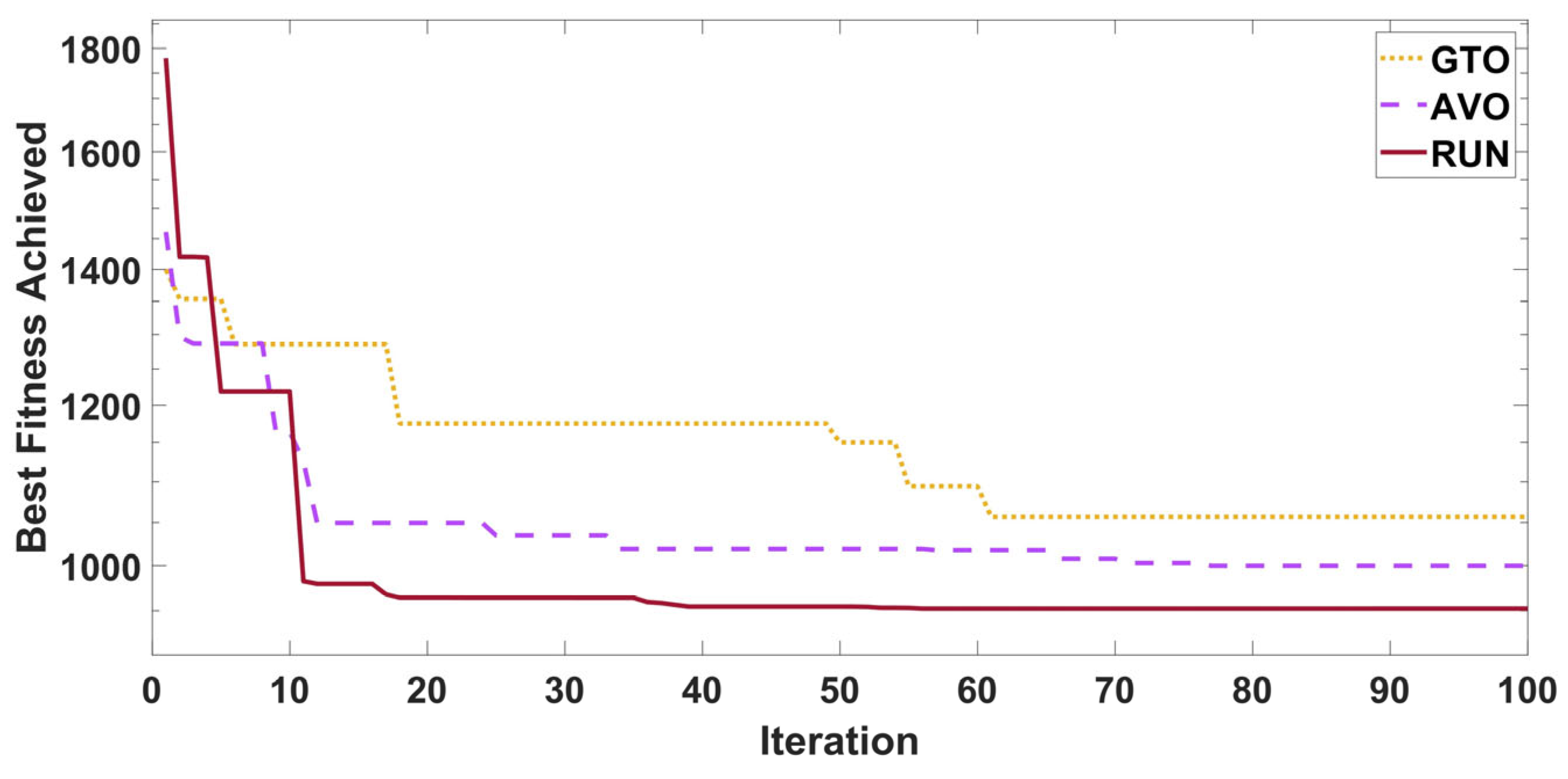
• Superior performance compared to other recent algorithms such as the GTO and AVO, as demonstrated through comparative simulations.

Additional comparisons have been made between the suggested FOPI-PI controller and its separate components (i.e., PI and FOPI), which are believed to be the controllers that are utilized the most in the majority of published works in this research area. The principal achievements of our work can be summarized in bullets as follows:

• The proposal of an innovative control strategy for MPPT in PV systems, named the IC-MPPT-(FOPI-PI) controller, which has been assessed and validated through MATLAB/Simulink simulations using a 100 kW benchmark PV system integrated into the grid;
• The first reported application of a new algorithm known as the RUNge Kutta Optimizer (RUN) to fine-tune the FOPI-PI controller parameters, comparing its performance with other recent metaheuristic optimization strategies like GTO and AVO to demonstrate the control scheme’s efficacy;
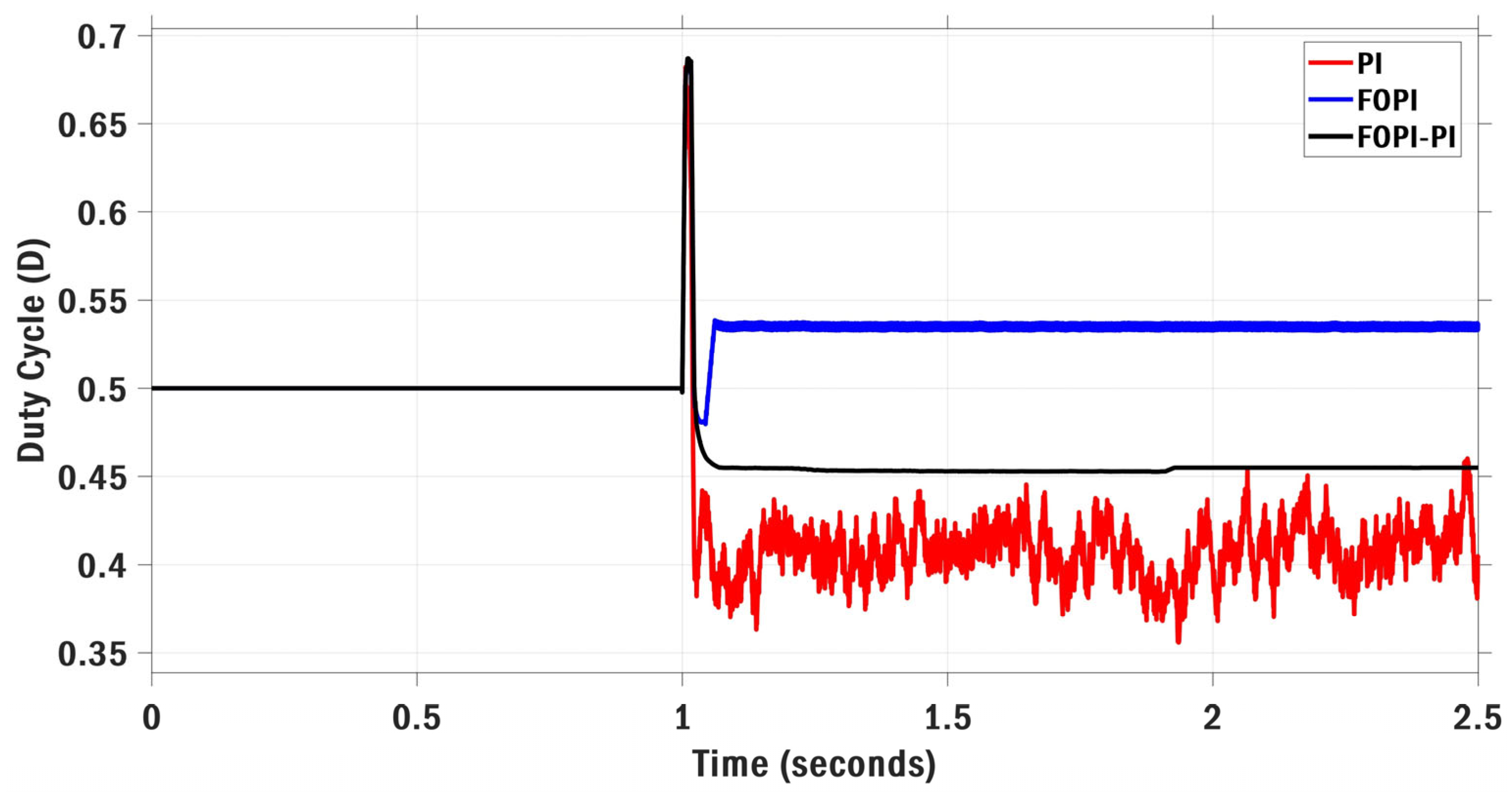
• The designed RUN-based IC-MPPT-(FOPI-PI) control strategy surpasses existing competitors in the MPPT research domain (PI [15] and FOPI [16] controllers) by precisely and efficiently tracking maximum power across diverse atmospheric conditions, including step, ramp, and realistic irradiance, considering constant and ramping temperature.

The remainder of the article has been structured as follows: Section 2 elucidates PV modeling and system setup. Additionally, Section 3 elucidates the IC-MPPT-(FOPI-PI) control approach. Furthermore, Section 4 illustrates the suggested RUN. Section 5 presents the simulation framework for the particular scenario under evaluation. Furthermore, Section 6 displays and analyzes the simulation outcomes. Finally, Section 7 includes the conclusion and future aspects.

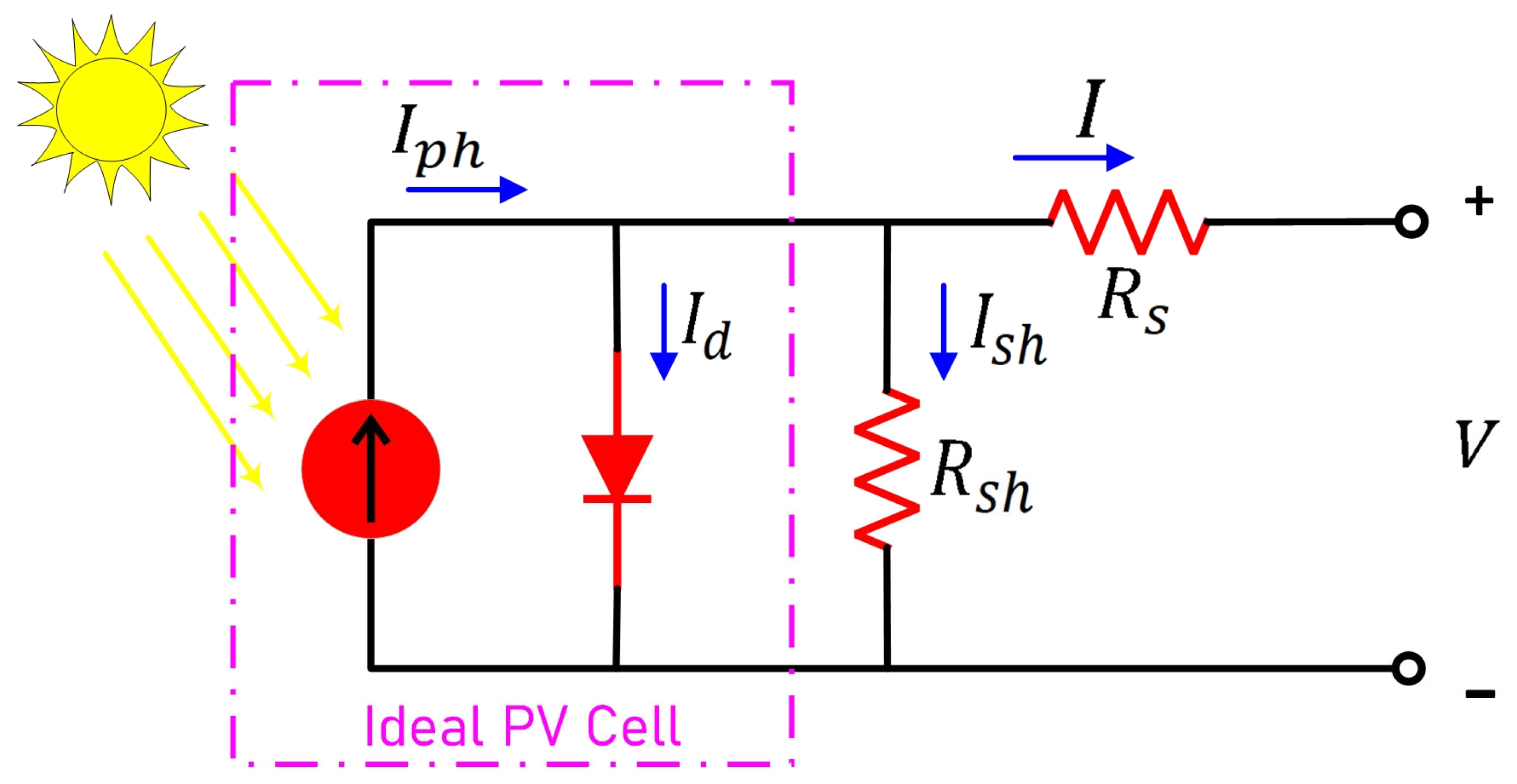
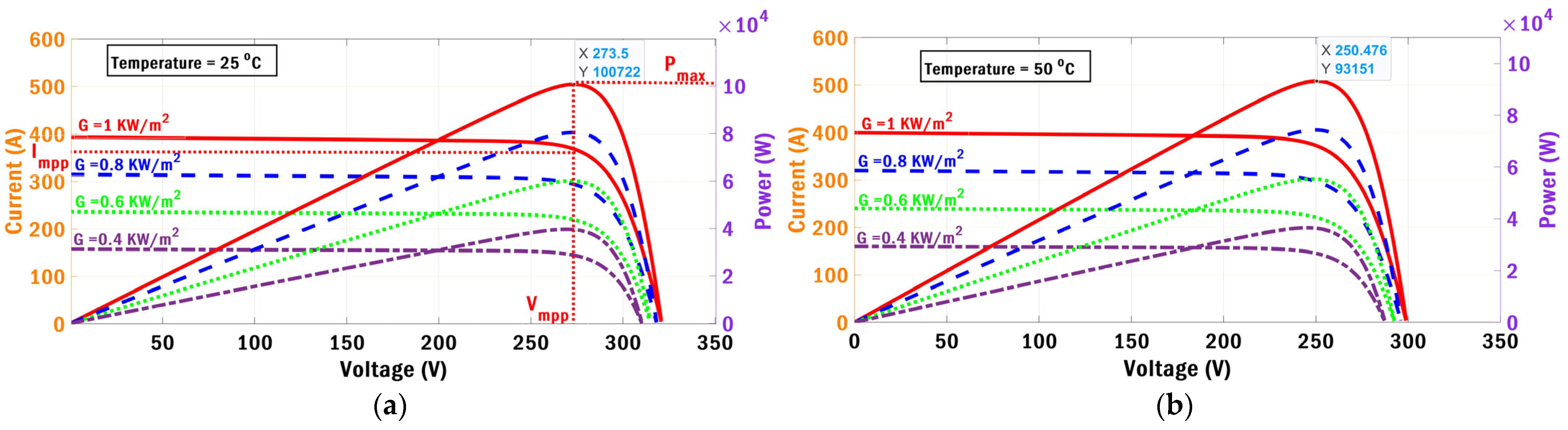
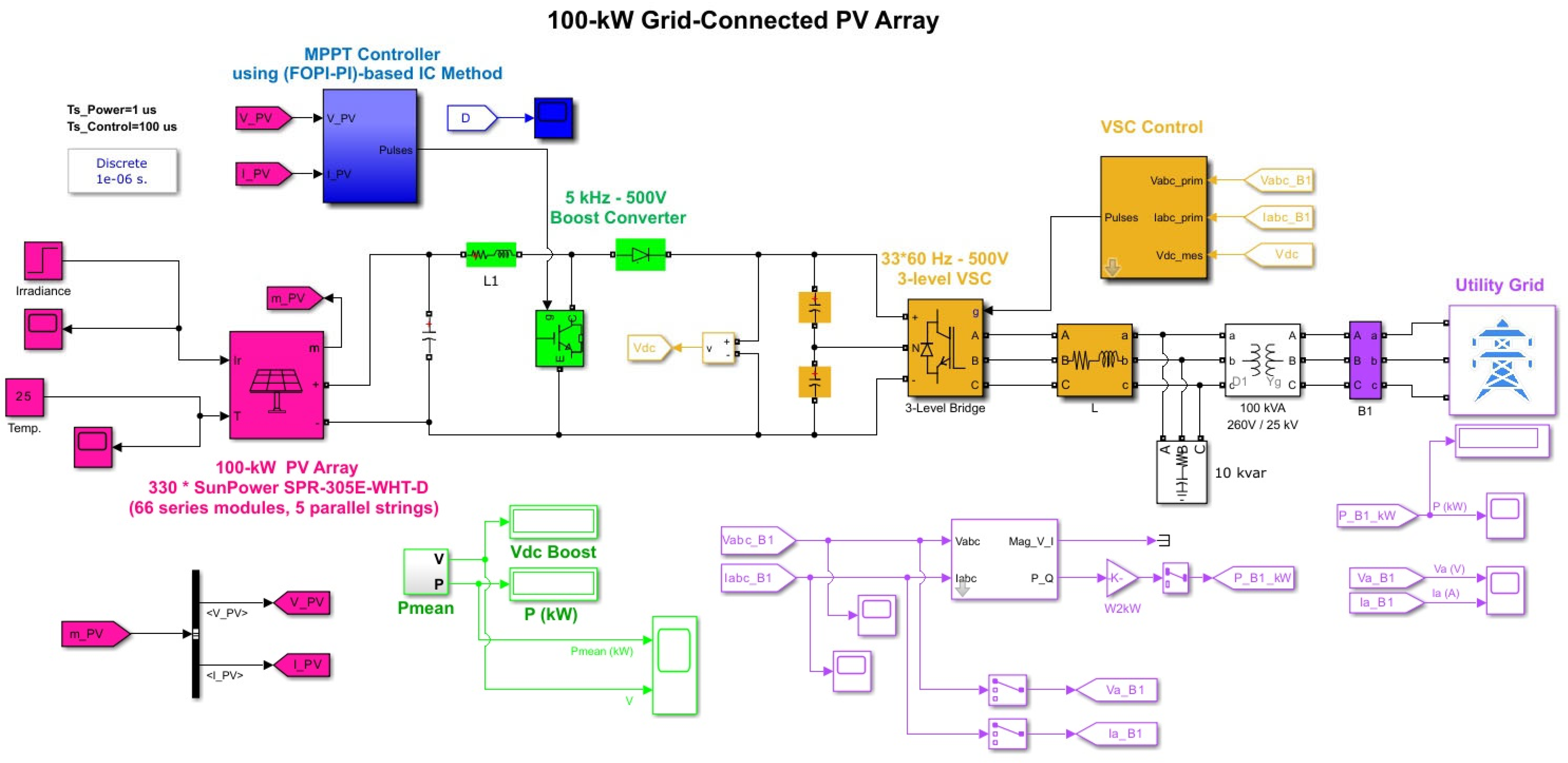
2. PV Modeling and System Setup

Several modeling approaches have been proposed by researchers to accurately simulate the behaviour of photovoltaic (PV) cells, among which the single diode model (SDM), double diode model (DDM), and triple diode model (TDM) are the most prominent [63]. Each of these models offers varying levels of complexity and accuracy, depending on the number of diodes and circuit elements incorporated. The TDM, while highly accurate, is computationally intensive, whereas the DDM provides a moderate balance between precision and complexity. However, the SDM stands out as the most commonly employed and computationally efficient model owing to its simple structure and implementation. It requires minimal parameter estimation, and is thus highly suitable for practical simulation and control applications [64].

The SDM denotes the PV cell using a single diode along with a current source, a series resistance, and a parallel (shunt) resistance. This structure enables it to effectively capture the essential electrical characteristics of a PV cell under varying environmental conditions with reasonable accuracy. Figure 1 represents the equivalent circuit of a photovoltaic cell under the SDM configuration. The electric performance of a PV module composed of multiple PV cells connected in series can be mathematically illustrated using a group of equations obtained from the SDM framework. These equations are labeled as Equations (1) through (6) [7].

$$I=I_{ph}-I_d-I_{sh}$$

(1)

$$I=I_{ph}-I_o\left(exp\left({\displaystyle \frac{V+R_{s}I}{a{N}_s{V}_t}}\right)-1\right)-{\displaystyle \frac{V+R_{s}I}{R_{sh}}}$$

(2)

$$V_t={\displaystyle \frac{K{T}_c}{q}}$$

(3)

$$I_{ph}={\displaystyle \frac{G}{G_n}}\left(I_{s{c}_n}+K_T\left(T_c-T_{c_n}\right)\right)$$

(4)

$$I_o=I_{o_n}{\left({\displaystyle \frac{T_c}{T_{c_n}}}\right)}^{3}exp\left({\displaystyle \frac{q{E}_g}{ak}}\left({\displaystyle \frac{1}{T_{c_n}}}-{\displaystyle \frac{1}{T_c}}\right)\right)$$

(5)

$$I_{o_n}={\displaystyle \frac{I_{s{c}_n}}{\mathit{exp}\left(\frac{V_{o{c}_n}}{a{N}_s{V}_{t_n}}\right)}}$$

(6)

Here, $I_{ph}$ depicts the current developed by sunlight, $I_d$ depicts the current of the Shockley diode, $I_{sh}$ stands for the current passing through the shunt resistance, $I_o$ depicts the diode’s saturation current, $V$ denotes the terminal voltage, $R_s$ represents the series resistance, $R_{sh}$ depicts the shunt resistance, $a$ denotes the idealist factor for diode $=0.94504$, $N_s$ stands for the series cells’ number, $V_t$ represents the thermal voltage, $K$ denotes the Boltzmann constant $=1.38\times {10}^{-23} \mathrm{J}/\mathrm{K}$, $T_c$ denotes the temperature, in Kelvin, of the PV cell, $q$ stands for electron charge $=1.6\times {10}^{-19} \mathrm{C}$, $G$ represents the solar irradiance, $I_{s{c}_n}$ is a representation of the short circuit current under standard test conditions (STCs), specifically represented by the symbol ($n$), which indicates that $G_n=1000 \mathrm{w}/{\mathrm{m}}^2, T_{c_n}=25 °\mathrm{C}$, $K_T$ stands for the temperature coefficient of $I_{sc}$, $E_g$ depicts the polycrystalline silicon’s bandgap energy $=1.12 \mathrm{e}\mathrm{V} @ 25 °\mathrm{C}$, and $V_{o{c}_n}$ represents the open circuit voltage.

The photovoltaic system being examined has a capacity of 100 kW. A total of 66 series-linked modules of the SunPower SPR-305E-WHT-D (SunPower Corporation, San Jose, CA, USA) category of product are situated inside each of the 5 shunt-linked strings that make up the photovoltaic array. The presented IC-MPPT-(FOPI-PI) control approach, is utilized to reduce the error signal of the conductance to achieve the highest possible output from the PV. Consequently, the FOPI-PI controller changes the duty cycle of the 500 V boost converter connected to the inverter associated with the medium voltage grid. Furthermore, the I–V and P–V interactions pertaining to several climatic weather conditions are described in Figure 2. One can note that temperature and irradiance are the driving forces behind the PV output [65]. The recommended methodology is depicted in the form of a schematic representation in Figure 3. Additionally, the details of the studied system can be found in [66].

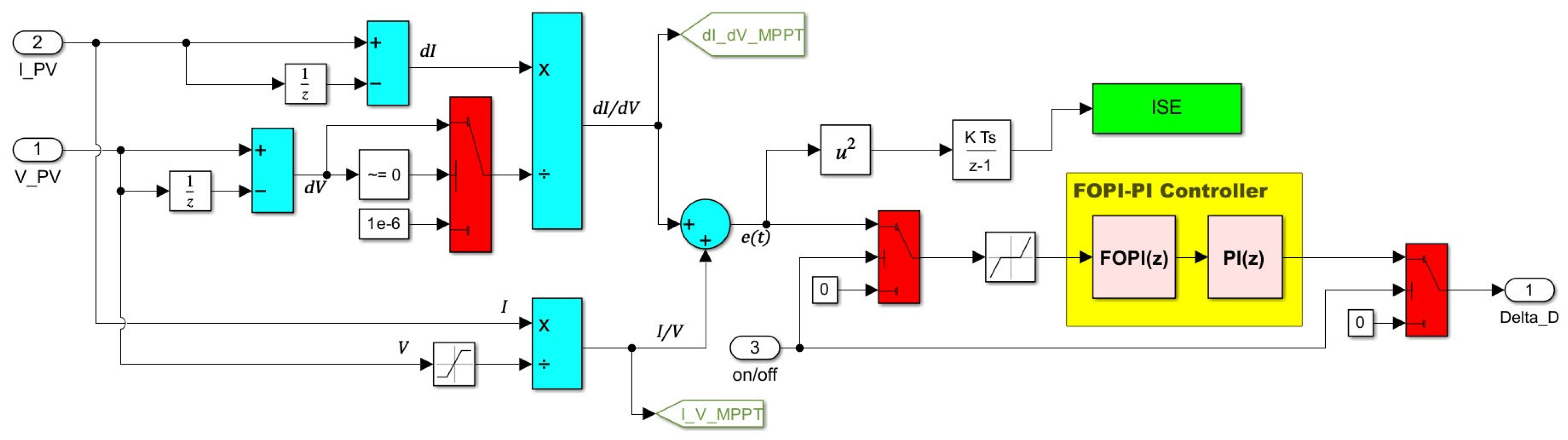
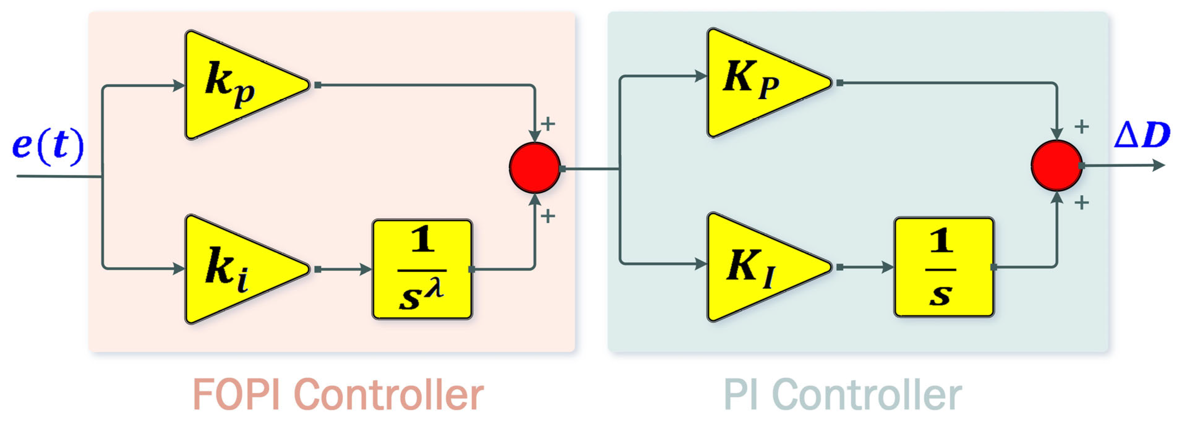
3. IC-MPPT-(FOPI-PI) Control Approach

Section 3 presents a thorough explanation of the suggested control strategy. The incremental conductance (IC) approach for tracking MPP has been integrated with the RUN-optimized FOPI-PI controller for the MPPT of a 100 kW grid-linked photovoltaic plant. The suggested FOPI-PI controller incorporates the characteristics of both fractional-order PI and conventional PI controllers. The FOPI controller, with its fractional-order integration, enhances the system’s ability to handle dynamic uncertainties and provides fine-tuned control over a broader frequency range. However, its computational complexity and sensitivity in real-time applications may limit its effectiveness when used alone. On the other hand, the classical PI controller offers a well-understood, robust, and computationally efficient control mechanism, particularly suited for handling steady-state error and ensuring system stability.

By cascading the FOPI and PI controllers, the proposed structure combines the fast transient response and adaptability of the FOPI controller with the steady-state robustness and simplicity of the conventional PI controller. This hybrid configuration enables the system to respond more effectively to rapid changes in irradiance and temperature while maintaining overall stability and reducing steady-state error. Furthermore, the integrated controller enhances MPPT tracking performance by enabling faster and smoother convergence to the maximum power point (MPP), minimizing rise and settling times, and reducing transient overshoot and steady-state oscillations. Figure 4 illustrates the schematic depiction of the FOPI-PI-based IC-MPPT model. Furthermore, the architecture of the suggested FOPI-PI regulator is illustrated in Figure 5. It is important to note that the controller output in this architecture corresponds to a perturbation step (ΔD), which is added to a fixed initial duty cycle value of 0.5 to generate the final duty cycle signal applied to the DC-DC converter. This fixed base value serves as a neutral starting point that balances the converter’s operation in a typical operating region, especially during initialization or prior to dynamic tracking. This mid-range value ensures that the DC-DC converter begins operation away from saturation or extreme conduction states, allowing the perturbation-based control (ΔD) to adjust in either direction (increase or decrease) depending on real-time MPP tracking needs. This method simplifies implementation while maintaining control responsiveness.

Having an optimally calibrated FOPI-PI controller necessitates deciding the optimum values of the five parameters ($k_p$, $k_i$, $\lambda$, $K_P$, $K_I$). The transfer function representation of the FOPI-PI regulator is illustrated in Equation (7). The Integral of Squared Error (ISE) criterion, as delineated in Equation (8), was utilized as the fitness function for the optimization of the FOPI-PI regulator. The ISE index reduces the error signal $e\left(t\right)$ generated by the IC approach so as to ensure optimal MPPT performance.

$$C\left(s\right)=(k_p+{\displaystyle \frac{k_i}{s^{\lambda }}})(K_P+{\displaystyle \frac{K_I}{s}})$$

(7)

$$Minimize ISE={\int }_0^{T_{ss}}{e}^2\left(t\right) dt$$

(8)

where $T_{ss}$ denotes the steady state time response and $e(t)={\displaystyle \raisebox{1ex}{$dI\left(t\right)$}\!\left/ \!\raisebox{-1ex}{$dV\left(t\right)$}\right.}+{\displaystyle \raisebox{1ex}{$I\left(t\right)$}\!\left/ \!\raisebox{-1ex}{$V\left(t\right)$}\right.}$.

During the process of optimization, the five parameters of the recommended FOPI-PI controller that has been described have been limited between upper limits (UL) and lower limits (LL) in accordance with Equation (9),

$$\left\{\begin{array}{c}\begin{array}{c}{k_p}_{LL}\le k_p\le {k_p}_{UL}\\ {k_i}_{LL}\le k_i\le {k_i}_{UL}\end{array}\\ {\lambda }_{LL}\le \lambda \le {\lambda }_{UL}\\ {K_P}_{LL}\le K_P\le {K_P}_{UL}\\ {K_I}_{LL}\le K_I\le {K_I}_{UL}\end{array}\right.$$

(9)

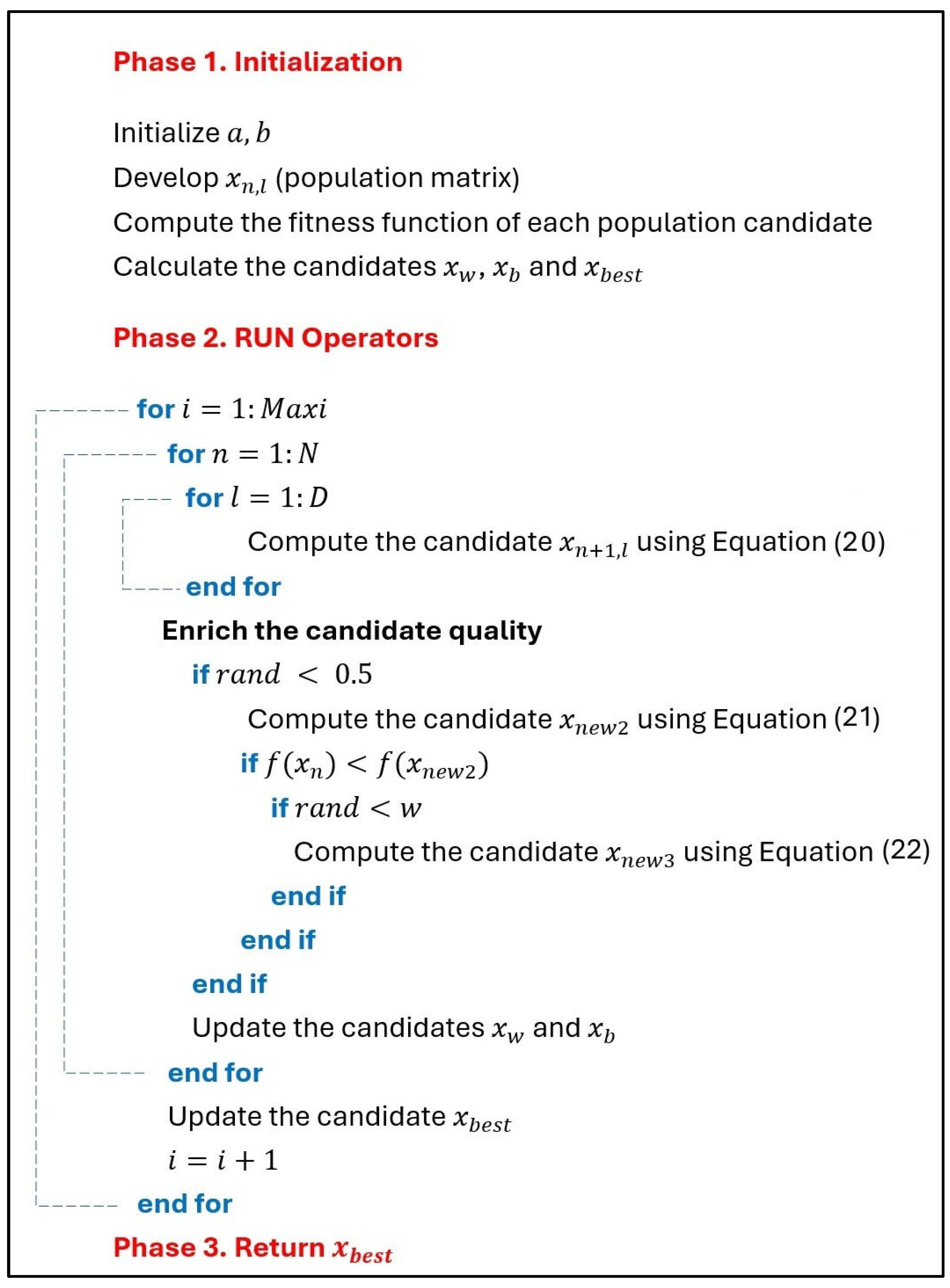
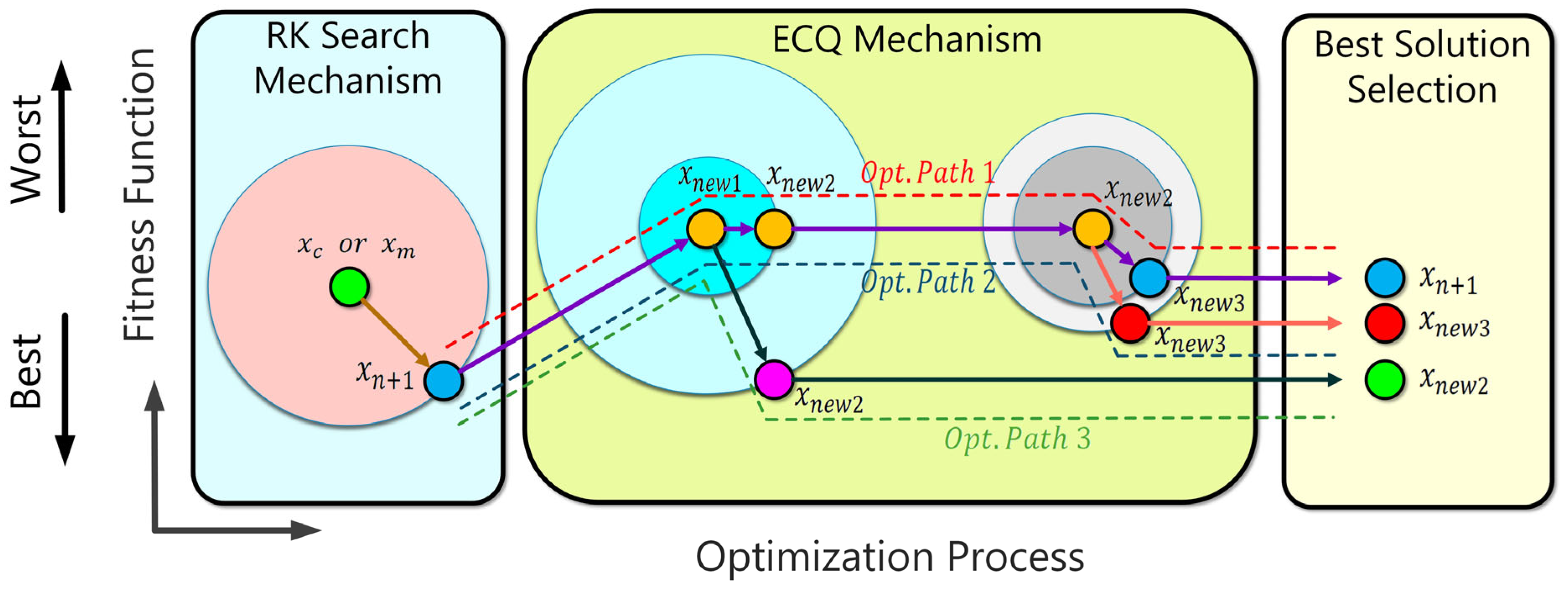
4. RUN Optimization Description

The RUN algorithm integrates the fundamental principles of the Runge–Kutta (RK) method with a population-inspired evolutionary methodology involving a collective of agents. Specifically, it utilizes the RK4 technique, a widely recognized numerical method, to accurately calculate slopes and solve ordinary differential equations [58]. This unique combination forms the core of RUN’s optimization strategy. The main idea behind RUN revolves around leveraging the slope estimates generated by the RK method as a heuristic guide. These slope computations are employed to systematically explore promising regions within the search space, effectively steering the search process toward optimal solutions. By incorporating this slope information, RUN establishes a set of evolutionary rules that govern the behavior and interaction of the population of agents. This approach aligns with the foundational concepts of swarm-based optimization algorithms, where collective intelligence and cooperative dynamics drive the search process. A detailed theoretical explanation of the RUN algorithm, including its mechanisms and operational principles, is provided in the following subsections to offer a comprehensive understanding of its design and functionality.

4.1. Population Initialization

This stage focuses on initializing the swarm that will evolve over the course of the specified number of iterations. In the RUN algorithm, a population consisting of $N$ individuals is randomly generated within the defined search space. Each member of this population, $x_n (n=1, 2,\dots , N)$, denotes a potential candidate for use in the optimization issue. Each solution is characterized by a dimensionality, $D$, corresponding to the number of decision variables involved in the problem. This initial random distribution of solutions provides a diverse starting point, enabling the approach to efficiently discover the search space from multiple directions. The beginning placements are generally generated arbitrarily based on the concept

$$x_{n,l}=L_l+rand.(U_l-L_l)$$

(10)

where $L_l$ and $U_l$ depict the lower and upper limits of the $l^{th}$ variable of the issue $(l=\mathrm{1,2},\dots ,D)$, and $rand$ represents an arbitrary number within the zero to unity range. This idea produces candidates within specified boundaries.

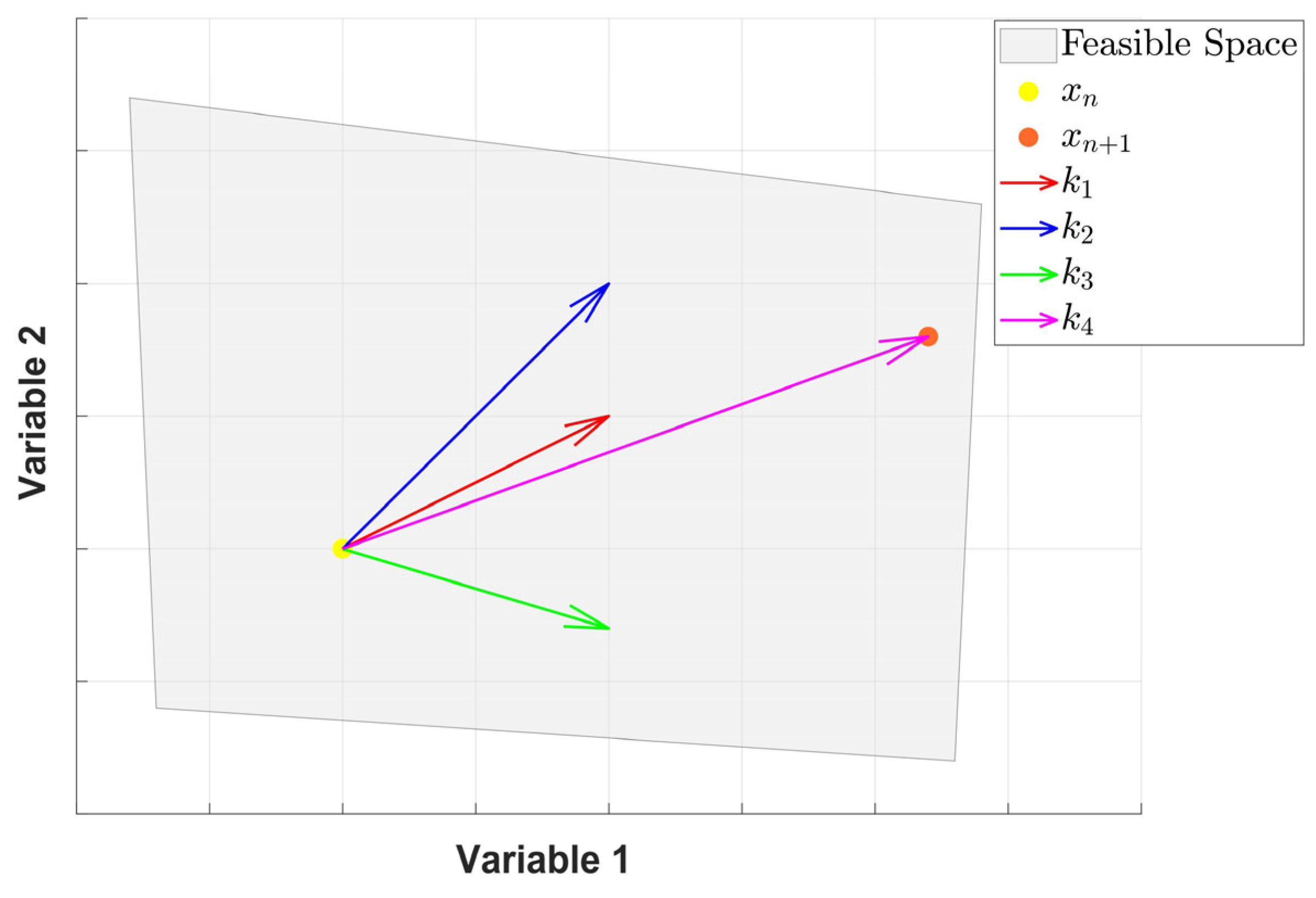
4.2. The Mathematical Description of Searching Methodology

The efficacy of any optimization algorithm fundamentally depends on its iterative mechanisms that balance exploration and exploitation processes. In the exploration phase, the approach generates a diverse set of arbitrary candidates that exhibit a high level of arbitrariness and variability. This diversity permits the algorithm to thoroughly investigate different promising regions within the feasible search space, enhancing the chances of locating the global optimum. In contrast, the exploitation phase involves more subtle and incremental adjustments to existing solutions, with significantly less randomness, focusing on refining and improving solutions in the vicinity of identified promising regions [58].

In this study, the primary search strategy of the RUN algorithm is employed, which harnesses the Runge–Kutta (RK) method to navigate the decision space. By generating and evolving a population of random candidate solutions, RUN effectively balances both global exploration and local exploitation. This approach enables comprehensive searching across the entire solution space while simultaneously allowing fine-tuned optimization around the best-performing regions, thereby improving the overall search efficiency and convergence performance.

The RK4 approach has been utilized so as to ascertain the search mechanism in the suggested RUN. The first-order derivative was employed to determine the coefficient $k_1$, derived using the following equation:

$$k_1=y^{\prime }(x)={\displaystyle \frac{y(x+\mathsf{\Delta }x)-y(x-\mathsf{\Delta }x)}{2\mathsf{\Delta }x}}$$

(11)

The suggested RUN utilizes location $x_n$ rather than its fitness $y\left(x_n\right)$, as evaluating the objective function for a position requires significant computational time. As per Equation (11), $x_n+∆x$ and $x_n-∆x$ represent two adjacent places of $x_n$. Considering $y\left(x\right)$ as a minimization issue, the locations $x_n-∆x$ and $x_n+∆x$ represent the optimal and suboptimal positions, respectively. Consequently, to formulate a population-based method, the location $x_n-∆x$ corresponds to $x_b$ (indicating $x_b$ is the optimal position around $x_n$), whereas the position $x_n+∆x$ corresponds to $x_w$ (indicating $x_w$ is the worst location surrounding $x_k$). Consequently, $k_1$ is defined as

$$k_1={\displaystyle \frac{x_w-x_b}{2\mathsf{\Delta }x}}$$

(12)

where $x_w$ and $x_b$ represent the worst and best candidates identified at each iteration, chosen from three arbitrarily picked solutions from the population members ($x_{r1}$, $x_{r2}$, $x_{r3}$), where $r1$, $r2$, and $r3$ are distinct and not equal to $n$.

To improve the exploratory search and induce unpredictability, Equation (12) can be reformulated as

$$k_1={\displaystyle \frac{1}{2\mathsf{\Delta }x}}(rand\times x_w-u\times x_b)$$

(12a)

$$u=round (1+rand)\times (1-rand)$$

(12b)

where $rand$ denotes an arbitrary value between zero and unity. The optimal solution ($x_b$) is essential for identifying potential regions and progressing towards the global optimum. Consequently, within the context, an arbitrary parameter $u$ is introduced to amplify the influence of the optimal solution ($x_b$) throughout the optimization procedure. By incorporating this stochastic factor, the algorithm dynamically adjusts the emphasis placed on the best-known solution, promoting a more flexible and adaptive search. In Equation (13), $∆x$ may be defined by

$$∆x=2\times rand\times \mid Stp\mid$$

(13a)

$$Stp=rand\times \left(\left(x_b-rand\times x_{avg }\right)+\gamma \right)$$

(13b)

$$\gamma =rand\times \left(x_n-rand\times (u-l)\right)\times exp\left(-4\times {\displaystyle \frac{i}{ Maxi }}\right)$$

(13c)

where $∆x$ represents the positional increment, contingent upon the parameter $Stp$. The step size, denoted as $Stp$, is determined by the difference between the optimal solution $x_b$ and the average solution $x_{avg }$. The parameter $\gamma$ serves as a scaling factor based on the overall magnitude of the solution space, which gradually decreases exponentially as the optimization progresses. Here, $x_{avg }$ represents the mean value of all candidates per iteration. Utilizing the arbitrary values ($rand$) in Equations (13a)–(13c), the approach can generate increased diversification trends and identify diverse regions inside the search space. Consequently, the remaining three coefficients (i.e., $k_2$, $k_3$, and $k_4$) may be expressed as follows:

$$k_2={\displaystyle \frac{1}{2\mathsf{\Delta }x}}\left(rand\cdot \left(x_w+{rand}_1\cdot k_1\cdot \mathsf{\Delta }x\right)-\left(u\cdot x_b+{rand}_2\cdot k_1\cdot \mathsf{\Delta }x\right)\right)$$

(14)

$$\begin{array}{c}\\ k_3={\displaystyle \frac{1}{2\mathsf{\Delta }x}}\left(rand\cdot \left(x_w+{rand}_1\cdot \left({\displaystyle \frac{1}{2}}{k}_2\right)\cdot \mathsf{\Delta }x\right)-\left({ u.x}_b+{rand}_2\cdot \left({\displaystyle \frac{1}{2}}{k}_2\right)\cdot \mathsf{\Delta }x\right)\right)\\ \end{array}$$

(15)

$$k_4={\displaystyle \frac{1}{2\mathsf{\Delta }x}}\left(rand\cdot \left(x_w+{rand}_1\cdot k_3\cdot \mathsf{\Delta }x\right)-\left(u\cdot x_b+{rand}_2\cdot k_3\cdot \mathsf{\Delta }x\right)\right)$$

(16)

Here, ${rand}_1$ and ${rand}_2$ depict two arbitrary values between zero and unity. The variables $x_w$ and $x_b$ are defined in this research by the following:

$$\left\{\begin{array}{c}{x}_b=x_n and x_w=x_{bi} if f\left(x_n\right)<f\left(x_{bi}\right) \\ x_b=x_{bi} and x_w=x_n otherwise\end{array}\right.$$

(17)

Here, $x_{r1}$, $x_{r2}$, and $x_{r3}$ are three arbitrary candidates, the best of which is chosen as $x_{bi}$. Based on Equation (17), if the fitness of the present candidate ($f\left(x_n\right)$) surpasses that of $x_{bi}$, then the optimal and worst candidates ($x_b$ and $x_w$) are designated as $x_n$ and $x_{bi}$, correspondingly. Otherwise, these values correspond directly to $x_{bi}$ and $x_n$, correspondingly. As a result, the primary search process in the RUN algorithm may be characterized as follows:

$$\begin{gathered} SM={\displaystyle \frac{1}{6}}\left(x_{RK}\right)\cdot \mathsf{\Delta }x \\ {x}_{RK}=k_1+2k_2+2k_3+k_4 \end{gathered}$$

(18)

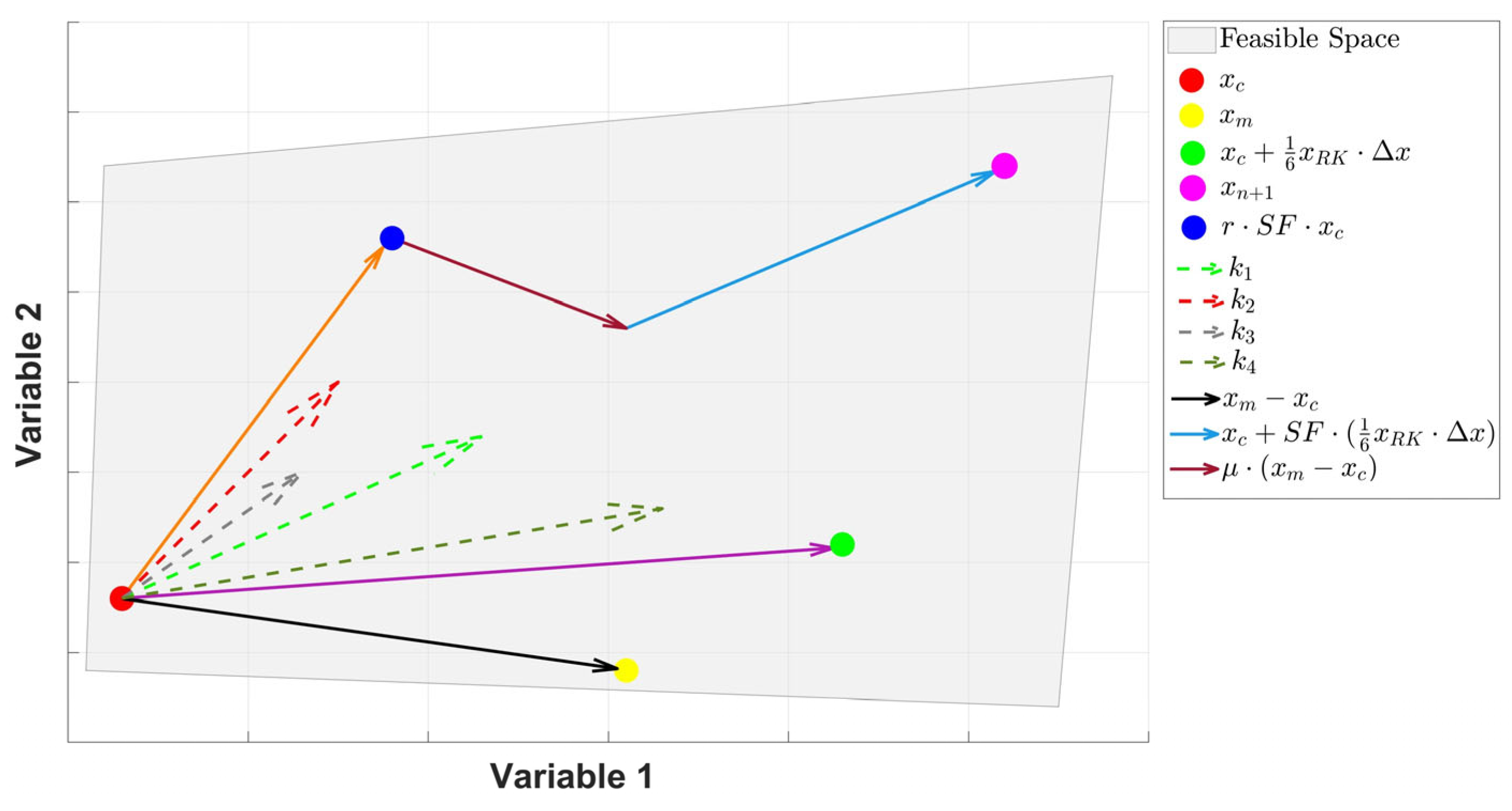
4.3. Updating Solutions

Starting with a random selection of solutions (candidates), the RUN algorithm optimizes the system. During each iteration, candidates adjust their places via the RK technique. So as to achieve this, RUN utilizes a candidate along with a search mechanism relying on the RK approach. The process by which a location is updated with the Runge–Kutta algorithm can be observed in Figure 6.

The RUN algorithm implements the following strategy to establish the location for the next iteration, facilitating both global (exploration) and local (exploitation) searches;

$$x_{n+1}=\left\{\begin{array}{c}Exploration Stage:x_c+SF\times SM+\mu \times x_{s1} , rand<0.5 \\ Exploitation Stage:x_m+SF\times SM+\mu \times x_{s2} , otherwise\end{array}\right.$$

(19)

in which

$$SF=2(0.5-rand)\times f$$

(19a)

$$f=a\times exp\left(-b\times rand\times {\displaystyle \frac{i}{ Maxi }}\right)$$

(19b)

$$\mu =0.5+0.1\times randn$$

(19c)

$$x_{s1}=randn\cdot (x_m+x_c)$$

(19d)

$$x_{s2}=randn\cdot (x_{r1}+x_{r2})$$

(19e)

$$x_m=\phi \times x_{best}+(1-\phi )\times x_{lbest}$$

(19f)

$$x_c=\phi \times x_n+(1-\phi )\times x_{r1}$$

(19g)

where $\mu$ represents an arbitrary number, $randn$ signifies an arbitrary number with a normal distribution, $\phi$ denotes a value within the range of zero to one, $x_{best}$ refers to the optimal candidate identified thus far, $x_{lbest}$ indicates the best candidate discovered during each iteration, and $SF$ represents an adaptive factor contingent upon two constants ($a$, $b$), $i$ stands for the current iteration number, and $Maxi$ depicts the maximum number of iterations.

This study utilized $SF$ to accomplish an appropriate equilibrium between exploration and exploitation. Based on Equation (19a), a high value of $SF$ is designated in the initial iterations to augment variety and improve exploration; thereafter, its value diminishes to boost exploitation by raising the iteration count. Equation (19) indicates that the suggested RUN determines the exploration and exploitation stages according to the criterion $rand<0.5$.

The innovative approach in RUN guarantees that when $rand<0.5$, a global search will be conducted across the entire solution space while concurrently doing a local search around the candidate solution $x_c$. By incorporating this innovative global exploration phase, RUN effectively probes the most favorable regions within the search space. If $rand \ge 0.5$, RUN performs a local search centered on the candidate $x_m$. This local search stage allows the method to significantly accelerate convergence and concentrate efforts on refining the most promising candidate solutions. To perform a local search around the candidates $x_c$ and $x_m$ and investigate the potential areas inside the search space, and Equation (19) is reformulated as

$$x_{n+1}=\left\{\begin{array}{c}Exploration Stage:{\left(1+r\times SF\times g\right) x}_c+SF\times SM+\mu \times x_{s1} , if rand<0.5 \\ Exploitation Stage:{\left(1+r\times SF\times g\right) x}_m+SF\times SM+\mu \times x_{s2} , otherwise\end{array}\right.$$

(20)

where $r$ denotes an integer, namely, either 1 or −1. This coefficient alters the search direction and enhances variety. $g$ depicts an arbitrary variable between zero and two. As stated in Equation (20), the local search surrounding $x_c$ diminishes with an increase in the number of iterations. Figure 7 illustrates the search mechanism of RUN, demonstrating the process for generating position $x_{n+1}$ in the subsequent iteration.

4.4. Enriched Candidate Quality (ECQ)

The RUN algorithm utilizes Enriched Candidate Quality (ECQ) to enhance candidate quality and prevent local optima in each iteration. Through the implementation of ECQ, the RUN optimization guarantees that each contender progresses towards a more advantageous position. The suggested ECQ computes the average of three arbitrary candidates ($x_{avg}$), and combines it with the optimal location ($x_b$) to create a new candidate ($x_{new1}$). The subsequent procedure is implemented to generate the candidate ($x_{new2}$) utilizing the ECQ:

$$x_{new2}=\left\{\begin{array}{c}{x}_{new1}+r\cdot w\cdot \left|\left(x_{new1}+x_{avg}\right)+randn\right|, (rand<0.5 \&\& w<1)\\ \left(x_{new1}-x_{avg}\right)+r\cdot w\cdot \left|\left(u\cdot x_{new1}+x_{avg}\right)+randn\right|, otherwise\end{array}\right.$$

(21)

in which

$$w=rand(\mathrm{0,2})\times exp\left(-c\times {\displaystyle \frac{i}{ Maxi }}\right)$$

(21a)

$$x_{avg}={\displaystyle \frac{x_{r1}+x_{r2}+x_{r3}}{3}}$$

(21b)

$$x_{new1}=\beta \times x_{avg}+(1-\beta )\times x_{best}$$

(21c)

where $\beta$ depicts an arbitrary value between zero and unity. $c$ denotes an arbitrary value, defined as $5\times rand$ in this research. $w$ denotes an arbitrary value that diminishes as the number of iterations increases. $r$ denotes an integer that can be negative one, zero, or positive one. $x_{best}$ denotes the optimal solution found till now. Based on the aforementioned approach, for $w<1$ (i.e., the later iterations), the candidate $x_{new2}$ tends to facilitate an exploitation search, whereas for $w \ge 1$ (i.e., the early iterations), the candidate $x_{new2}$ tends to promote an exploration search. In the latter situation, parameter $u$ is defined to enhance variety. It is significant that ECQ is implemented when the criterion $rand<0.5$ is satisfied. The candidate computed in this section ($x_{new2}$) may not exhibit superior fitness compared to the existing candidate (i.e., $f\left(x_{new2}\right)>f\left(x_n\right)$). A new candidate ($x_{new3}$) is created to provide an additional opportunity for formulating an effective candidate, characterized as

$$x_{new3}=\left(1-rand\right) x_{new2}+SF\cdot rand\cdot \left(x_{RK}+\left(v\cdot x_b-x_{new2}\right)\right) if rand<w$$

(22)

where $v$ is an arbitrary number valued at $2\times rand$. The novel candidate ($x_{new3}$) is executed when the condition $rand<w$ is satisfied. The primary aim of Equation (22) is to advance the candidate $x_{new2}$ to a more optimal location. The initial law of this expression generates a local search cantered on $x_{new2}$, whereas the subsequent rule involves RUN attempting to investigate potential areas by moving towards the optimal answer. Therefore, coefficient $v$ is employed to underscore the significance of the optimal solution. It is important to observe that in the computation of $x_{RK}$, the solutions $x_b$ and $x_w$ are designated as $x_k$ and $x_{new2}$, respectively, due to the fitness value of $x_n$ being inferior to that of $x_{new2}$ (i.e., $f\left(x_{new2}\right)>f\left(x_n\right)$). The pseudo-code for RUN is seen in Figure 8.

In RUN, three pathways are taken into account for optimization, as seen in Figure 9. The suggested technique initially utilizes the RK search mechanism to develop position $x_{n+1}$, subsequently applying the ECQ mechanism to investigate the potential areas inside the search space. This process indicates that RUN pursues three pathways to attain an improved candidate. In the first and second pathways, the candidate $x_{new2}$, computed by the ECQ, is juxtaposed with the location $x_{k+1}$. If the fitness value of $x_{new2}$ is inferior to that of $x_{k+1}$ (i.e., $f\left(x_{new2}\right)>f\left(x_{k+1}\right)$), a new candidate ($x_{new3}$) is produced. If $f\left(x_{new3}\right)<f\left(x_{n+1}\right)$, then the optimal candidate is $x_{new3}$ (second route). Alternatively, it is $x_{n+1}$ (initial path). If $f\left(x_{new2}\right)<f\left(x_{n+1}\right)$, then the optimal solution is $x_{new2}$.

5. Simulation Framework

The procedure of the simulation framework may be articulated in brief through the subsequent steps:

➢

Step 1. Choose the suitable number of search agents and maximum iterations for all three compared optimization methods (AVO, GTO and RUN);

➢

Step 2. Determine the appropriate upper and lower limits for the proposed FOPI-PI controller parameters ($K_P$, $K_I$, $k_p$, $k_i$, $\lambda$) to ensure precise and rapid performance;

➢

Step 3. Designate ISE as a fitness function derived from Simulink;

➢

Step 4. Execute AVO, GTO and RUN on the PV simulation model within the aforementioned constraints;

➢

Step 5. Update the best-found controllers’ parameters, which score the lowest ISE, during the iterative process of the optimization;

➢

Step 6. Following the last iteration of the optimization, we can derive the most optimal settings of the three compared controllers for the efficient extraction of photovoltaic output power.

Table 1. The setting of the optimization methods’ parameters.

Optimization	Parameters	Value	Max Iteration	Search Agents	Boundary Limits
RUN	H	0.9	100	30	$\begin{array}{c}0\le K_P\le 1\\ 0\le K_I\le 2\\ 0\le k_p\le 4\\ 0\le k_i\le 4\\ 0\le \lambda \le 1\end{array}$
	k1	0.2
	k2	0.5
	k3	0.7
	k4	0.3
	r1, r2, μ, β	[0:1]
AVO	A	1.9	100	30
	b	1.1
	r1, r2, r3	[0:1]
GTO	p	0.25	100	30
	c	1.2
	r1, r2	[0:1]

enumerates the parameters selected for the evaluated optimization methods. Additionally,

Table 2. The detailed settings of the simulation platform.

Feature	MATLAB/SIMULINK R2024b
Sampling control step	${10}^{-4}$ s
Solver type	Discrete-fixed step (auto)
Powergui	Discrete with ${10}^{-6}$ s sampling time
Processor	AMD Ryzen 7 3700U with Radeon, 2.30 GHz

outlines the particulars of the simulation platform.

6. Results and Discussion

By utilizing a suggested optimization Runge-Kutta, the proposed controller FOPI-PI was compared with its components (i.e., FOPI and PI controllers) to demonstrate the high performance of suggested controller in tracking maximum power, rising time, settling time, and overshoot. The PV system under the impact of the suggested IC-MPPT-(FOPI-PI) control strategy is tested using five different climate scenarios that can be summarized as follows:

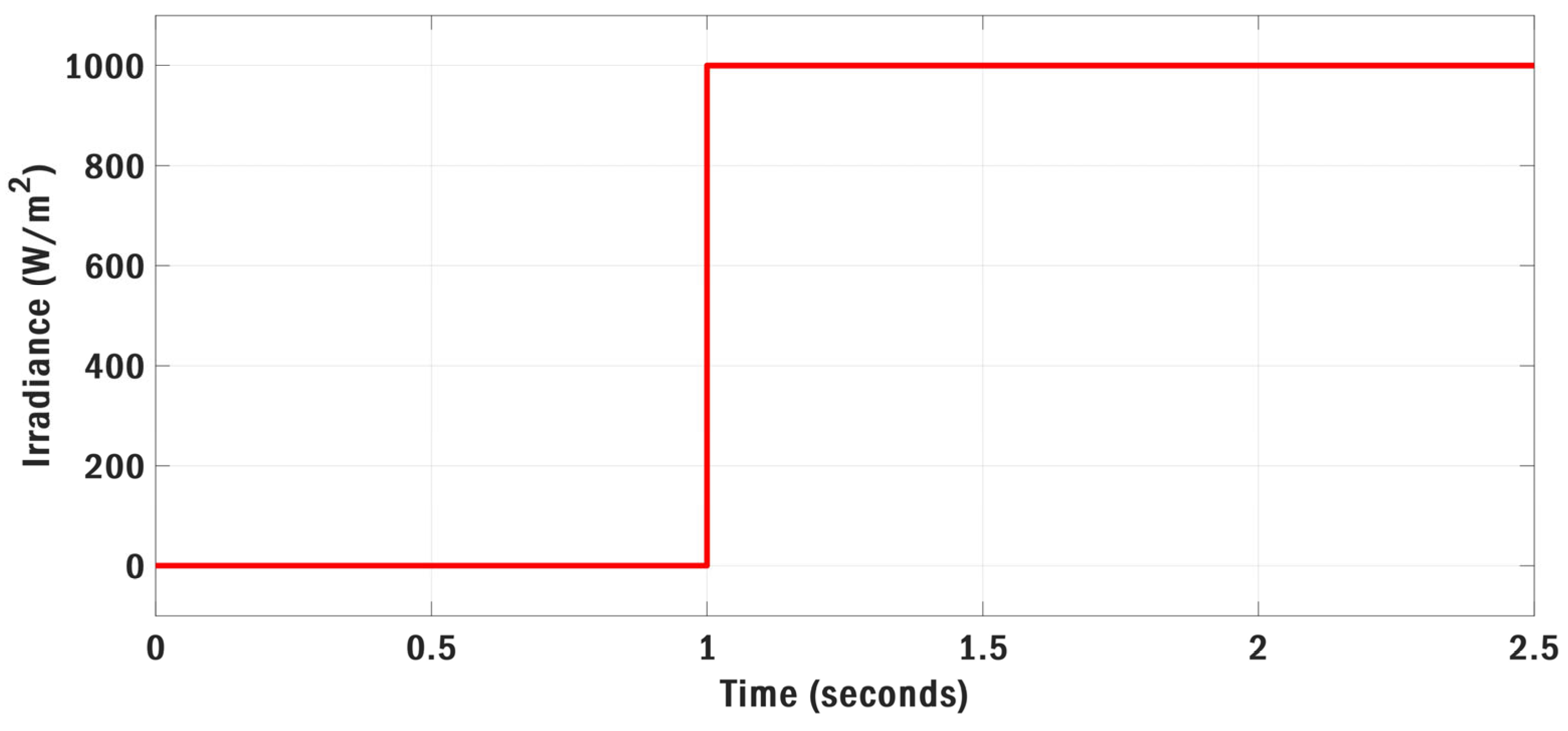
• Scenario I: Stepwise irradiance variation with constant temperature.
• Scenario II: Ramp irradiance and temperature variations.
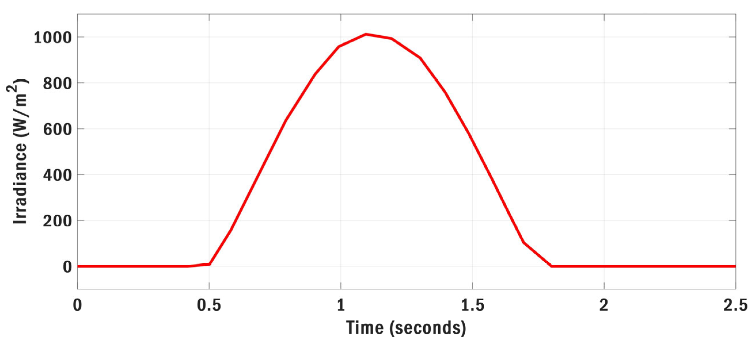
• Scenario III: Realistic irradiance variation with constant temperature.
• Scenario IV: Realistic irradiance and temperature variations.
• Scenario V: Multi-stepwise irradiance and temperature variations.

Initially, to illustrate the efficiency of the proposed RUN approach in optimizing the three examined controllers, a comparison has been conducted, under the influence of scenario I, between the RUN, AVO, and GTO algorithms. Figure 10 describes the convergence curves (best fitness vs iterations) of the three techniques under comparison. In comparison to the FOPI-PI control strategies based on AVO and GTO, which yielded fitness function (ISE) scores of 1000 and 1056, respectively, the FOPI-PI controller’s RUN score of 952 is the lowest. The optimal parameters of the FOPI-PI regulator derived from the three comparative methods are presented in

Table 3. Optimal parameters of FOPI-PI controller using RUN, AVO and GTO.

Optimization	PI		FOPI
	${\mathit{K}}_{\mathit{P}}$	${\mathit{K}}_{\mathit{I}}$	${\mathit{k}}_{\mathit{p}}$	${\mathit{k}}_{\mathit{i}}$	$\mathit{\lambda }$
RUN	0.081	0.423	3.992	3.439	0.837
AVO	0.057	0.893	3.148	2.826	0.258
GTO	0.035	0.367	3.739	3.952	0.355

.

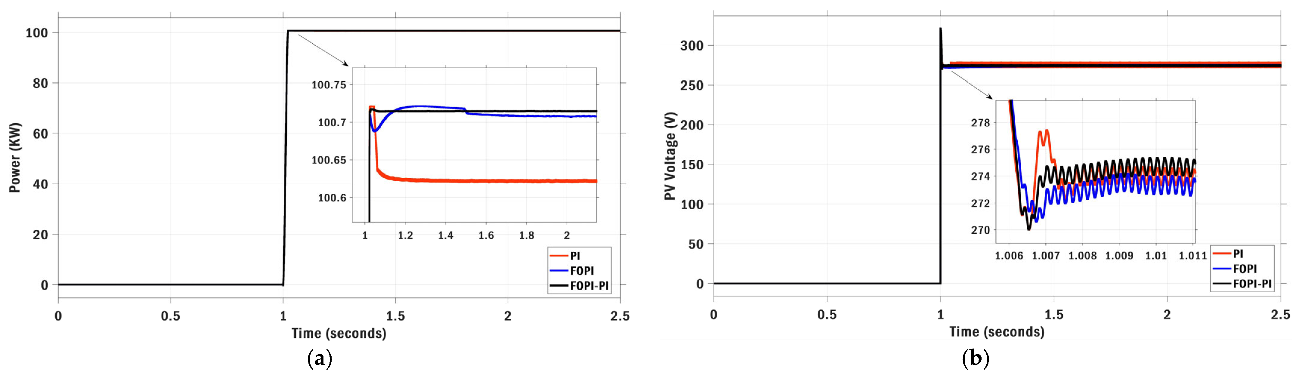
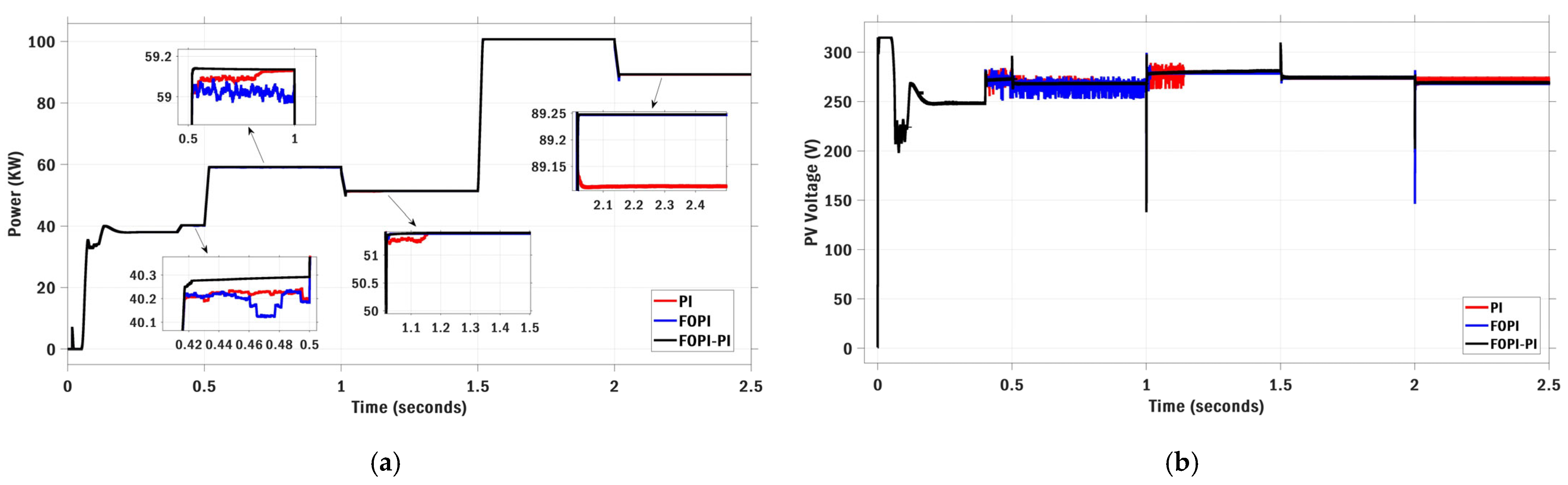
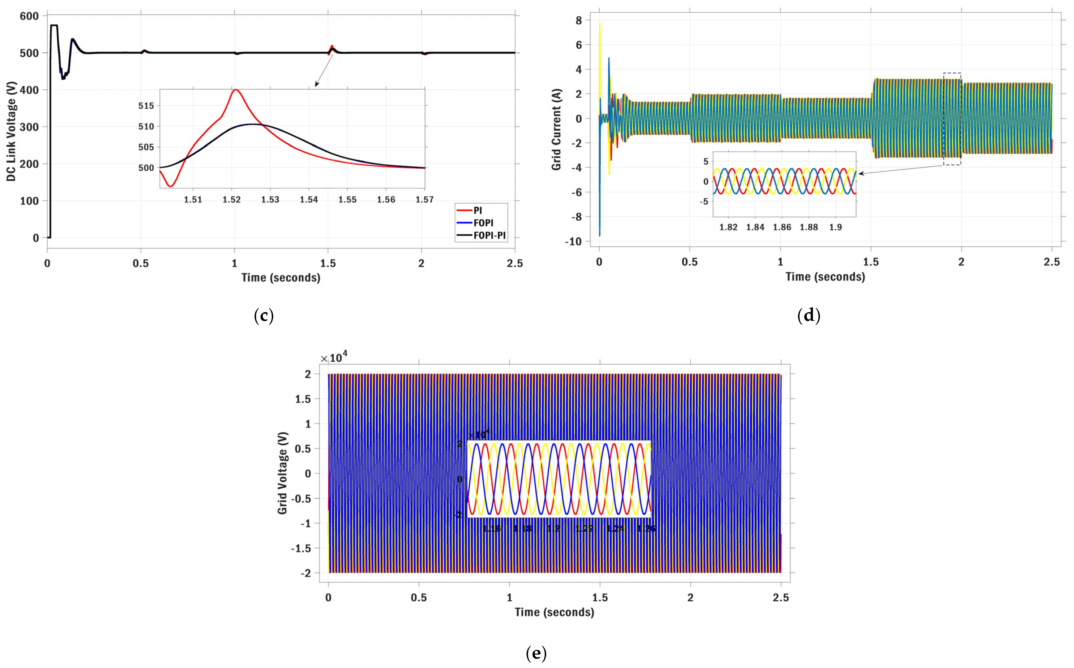
6.1. Scenario I: Stepwise Irradiance Variation with Constant Temperature

For the first scenario, a step pattern for irradiance is adopted with a step time of one second and final value of 1000 $\mathrm{W}/{\mathrm{m}}^2$, as seen in Figure 11, considering a constant temperature of 25 $°\mathrm{C}$. Figure 12 illustrates the impact of each control strategy on the resulting duty cycle in this case. It is evident that the duty cycle behavior varies significantly depending on the employed algorithm. Specifically, the PI controller produces duty cycle values that oscillate around 0.4, while the FOPI controller results in smaller oscillations centered around 0.54. In contrast, the proposed FOPI-PI controller maintains a more stable response, with the duty cycle converging toward an almost steady-state value of approximately 0.45.

Table 4. Optimal parameters of FOPI-PI, FOPI and PI controllers via RUN algorithm.

Controller	PI		FOPI
	${\mathit{K}}_{\mathit{P}}$	${\mathit{K}}_{\mathit{I}}$	${\mathit{k}}_{\mathit{p}}$	${\mathit{k}}_{\mathit{i}}$	$\mathit{\lambda }$
FOPI-PI (Proposed)	0.081	0.423	3.992	3.439	0.837
FOPI	--	--	0.476	0.071	0.543
PI	0.511	1.411	--	--	--

displays the optimal parameters of the three compared controllers (i.e., PI, FOPI, and FOPI-PI) obtained via the RUN algorithm. From

Table 5. The IC-MPPT-based PV system dynamics with the integration of the three different controllers for Scenario I.

Controller	Fitness Value (ISE)	T-Rising (Seconds)	T-Settling (Seconds)	P-Maximum (KW)	Overshoot Percentage	Efficiency %
FOPI-PI (Proposed)	16.781	0.0012	0.015	100.714	0.0109	99.984
FOPI	16.829	0.0013	0.094	100.708	0.0198	99.978
PI	17.442	0.0013	0.084	100.622	0.0158	99.893

, it is made clear that FOPI-PI provides the finest Runge–Kuta PV power performance since it takes the shortest settling time (0.015 s), which is deductively less than those of other rivals. Additionally, the maximum power gained from FOPI-PI is 100.714 kW, with FOPI coming in second at 100.708 kW and PI third at 100.622 kW. Among the others, FOPI-PI has the lowest overshoot percentage (0.0109%). Regardless, there is no appreciable variation in the rising time. However, the efficiency of the IC-MPPT has been raised to 99.984%. Moreover, the PV output voltage exhibits the softest response under the FOPI-PI control scenario. Figure 13a,b illustrate the PV power and voltage profiles corresponding to the optimized gain settings of the FOPI-PI, FOPI, and PI controllers, respectively. Meanwhile, Figure 13c depicts the DC link voltage, which is maintained at a steady reference level of 500 V. The voltage closely tracks this reference throughout the simulation, with only a slight overshoot occurring at $t=1$ s, coinciding with the step change in irradiance from zero to $1000 \mathrm{W}/\mathrm{m}²$. Concerning the power quality of the output signals on the grid side, Figure 13d,e illustrate the waveform shapes produced for both the grid current and voltage, respectively. There does not appear to be any significant harmonic impact on the output signals, as can be seen from the tiny, magnified areas of Figure 13d,e. Furthermore, it is worth observing that the optimal settings of the three regulators, as indicated in Table 4, derived from scenario I, were utilized to evaluate the four subsequent cases.

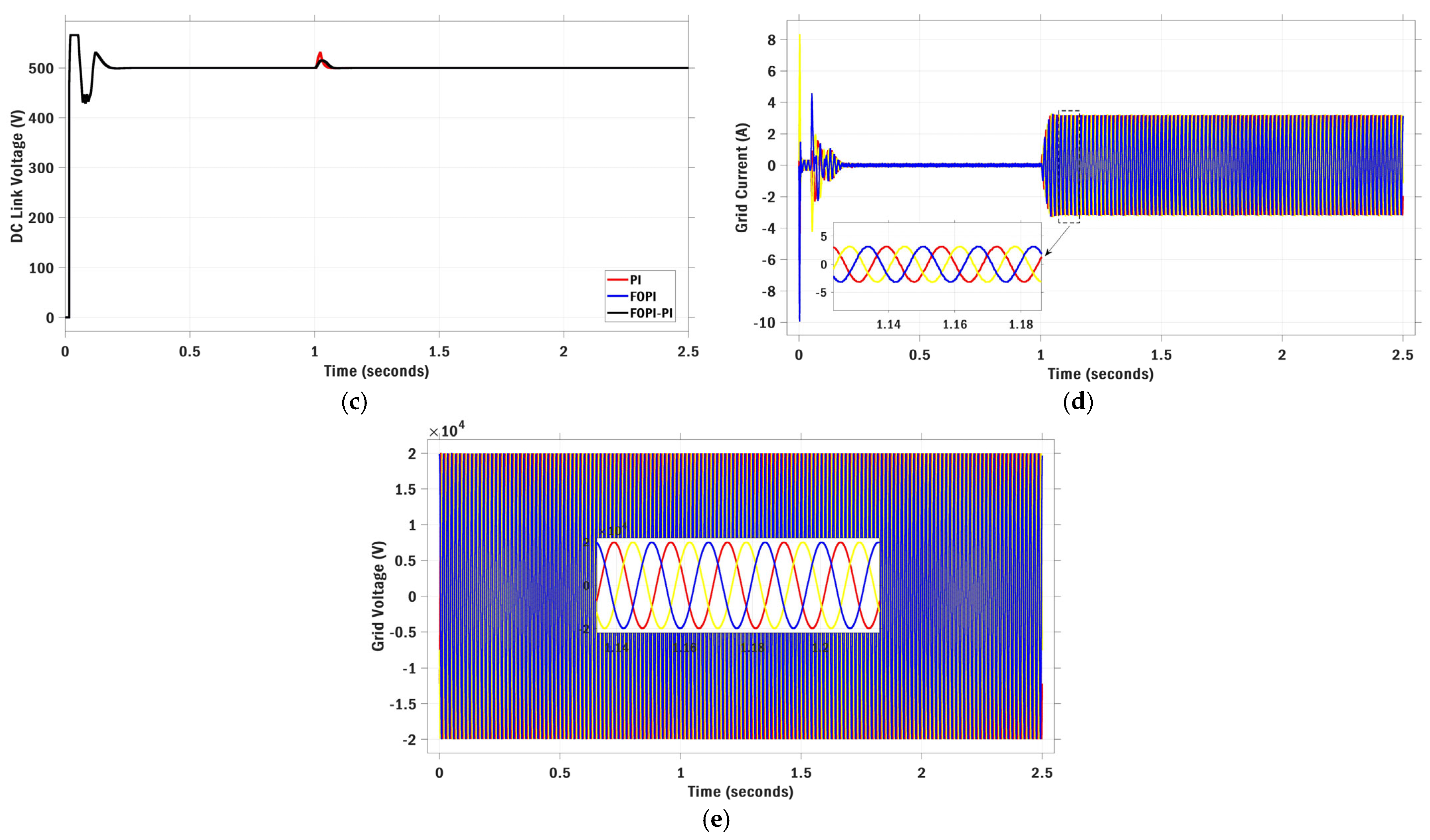
6.2. Scenario II: Ramp Irradiance and Temperature Variations

Regarding the second scenario, a ramp shape has been considered for both irradiance and temperature, as described in Figure 14a,b. One may observe from Figure 14a that temperature increased almost suddenly from the typical value ($25 °\mathrm{C}$) to $50 °\mathrm{C}$ at t = 2 s. On the other hand, as seen in Figure 14b, a drop occurred in irradiance from 1000 $\mathrm{W}/{\mathrm{m}}^2$ to 250 $\mathrm{W}/{\mathrm{m}}^2$, and this drop continued for a short time, then increased to the initial value again. Figure 15 compares the duty cycle responses generated by each control approach under these conditions. Figure 16a,b describe a detailed system dynamics’ assessment of the RUN-based FOPI-PI, FOPI, and PI regulators in terms of PV power and voltage, respectively. One can note that the PV system’s output power is directly proportional to the irradiance level and inversely related to the temperature. According to

Table 6. The IC-MPPT-based PV system dynamics under the integration of the three different controllers for Scenario II.

Controller	Fitness Value (ISE)	T-Rising (seconds)	T-Settling (seconds)	P-Maximum (KW)	Overshoot Percentage	Efficiency %
FOPI-PI (Proposed)	27.905	0.0017	0.02	100.721	0.0094	99.999
FOPI	53.471	0.0022	0.025	100.633	0.0496	99.905
PI	51.246	0.0019	0.03	100.715	0.0148	99.995

, the highest PV power was achieved via the IC-MPPT-(FOPI-PI) method, which was 100.721 kW with an MPP tracking efficiency of 99.999%, followed by PI at 100.715 kW with 99.995% efficiency, and FOPI at 100.633 kW with 99.905% efficiency. Furthermore, the most optimal and smooth response in the low-irradiance period is FOPI-PI, which is superior to those of FOPI and PI. Additionally, FOPI-PI has the lowest overshoot percentage of 0.0094%, which is 5 times lower than FOPI and 1.6 times lower than PI. Also, the proposed control methodology obtained the shortest rising and settling times (0.0017 and 0.02 s, respectively). Figure 16c describes the DC link voltage response, which is nearly the same for the three controllers compared. As seen in Figure 16d, the grid current closely tracks the irradiance design from $t=0$ to $t=2$ s as temperature remains constant. However, a slight decrease in current occurs at $t=2$ s, corresponding to an increase in temperature. Figure 16e shows the grid voltage, with a maximum phase voltage reaching 20 kV.

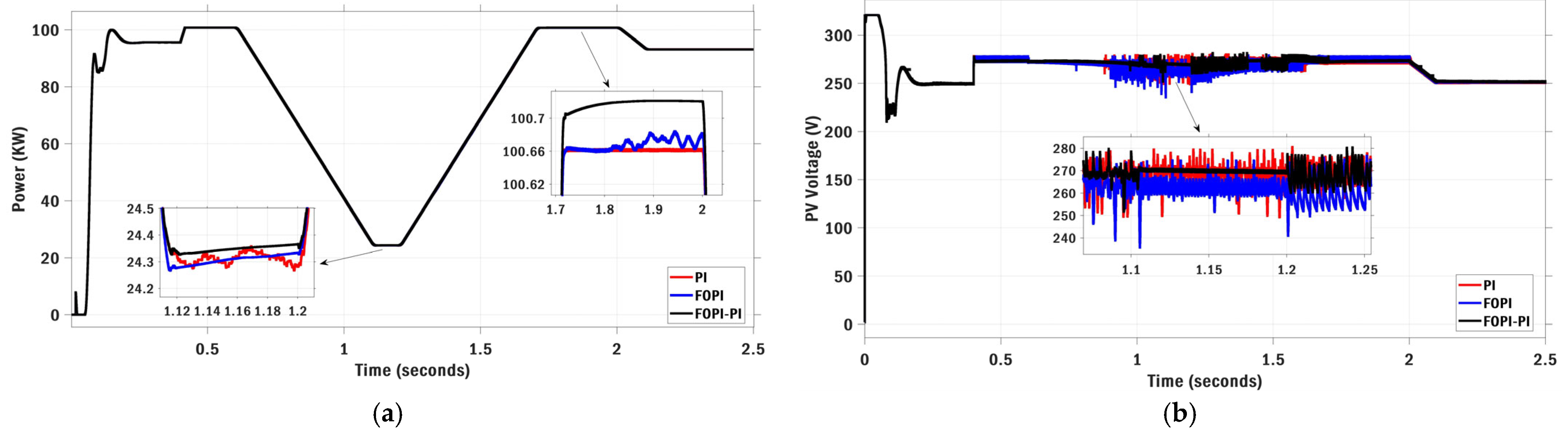
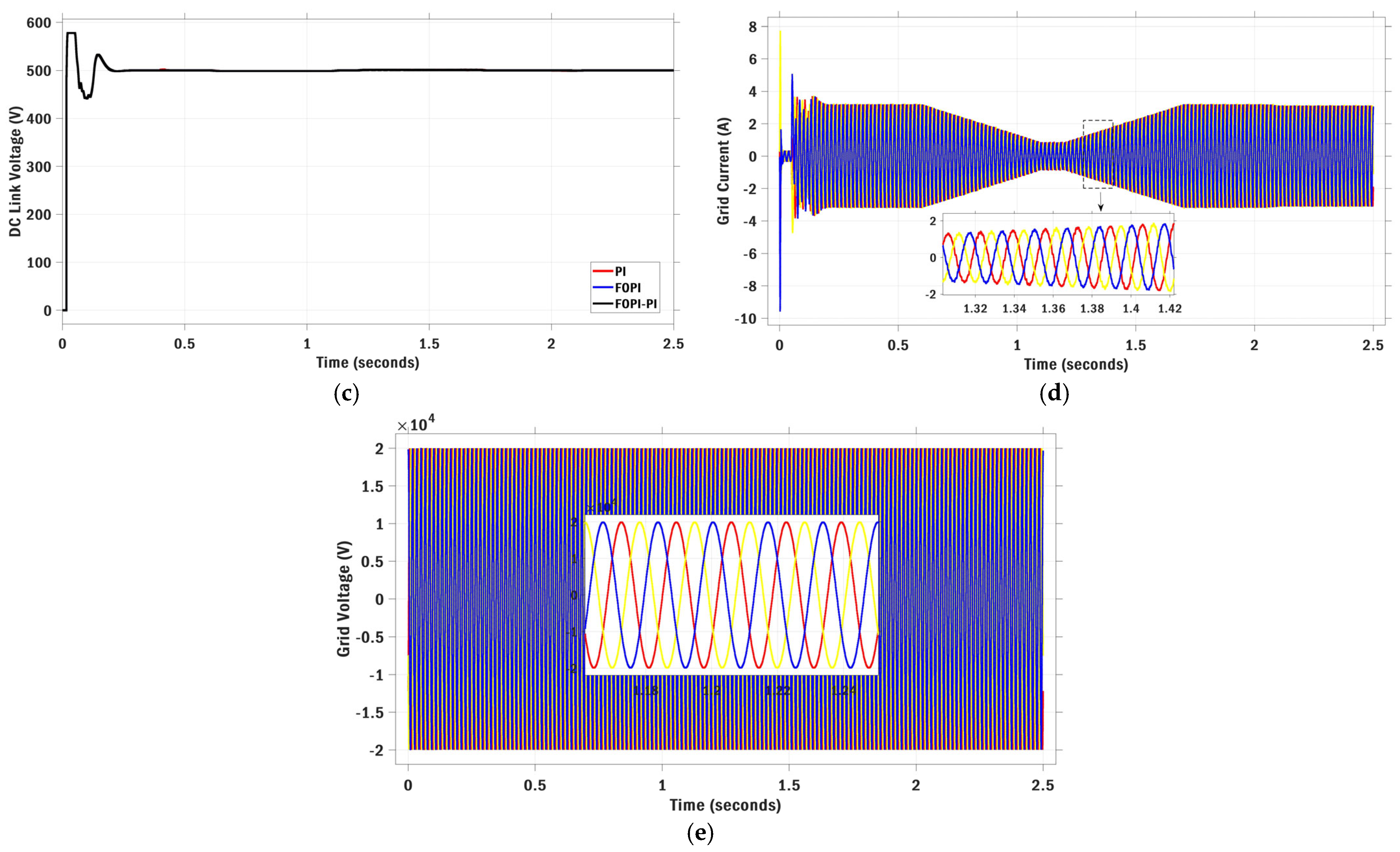
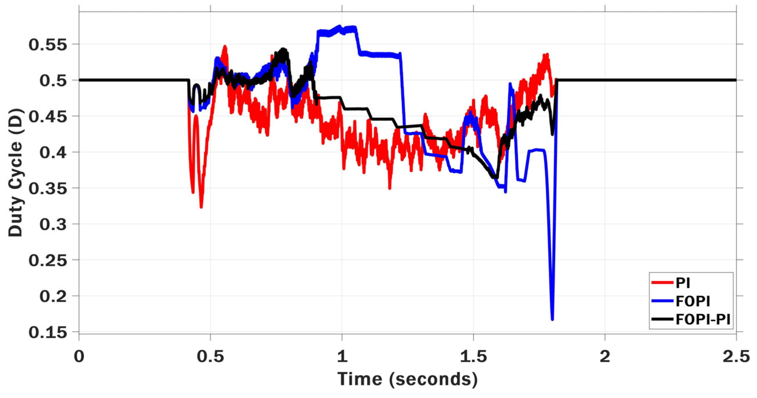
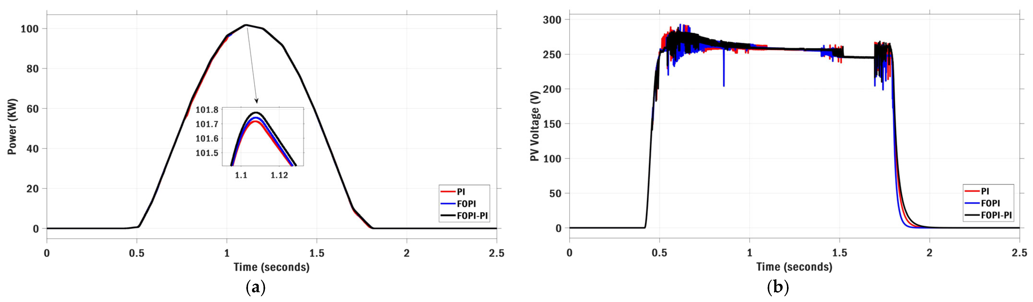
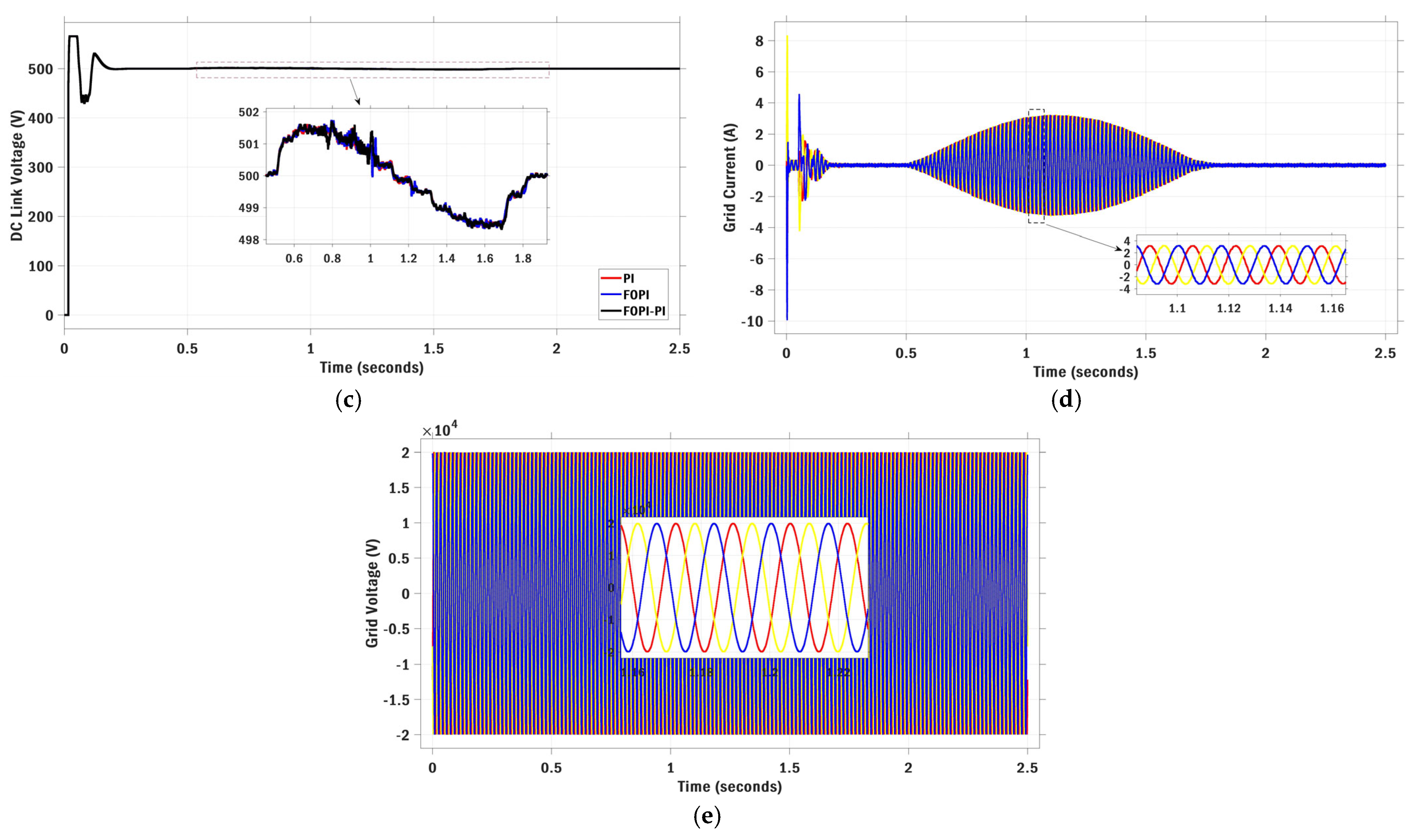
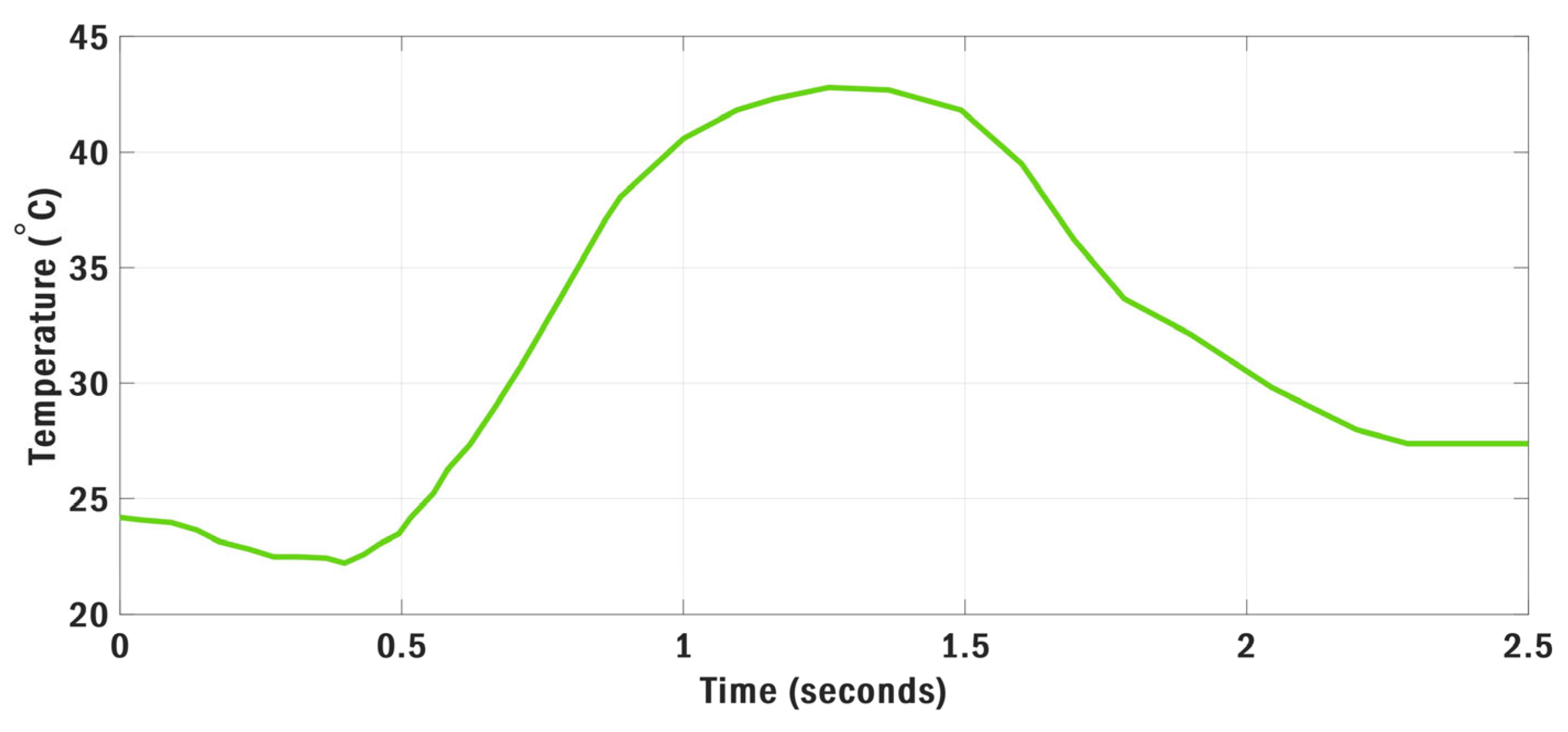
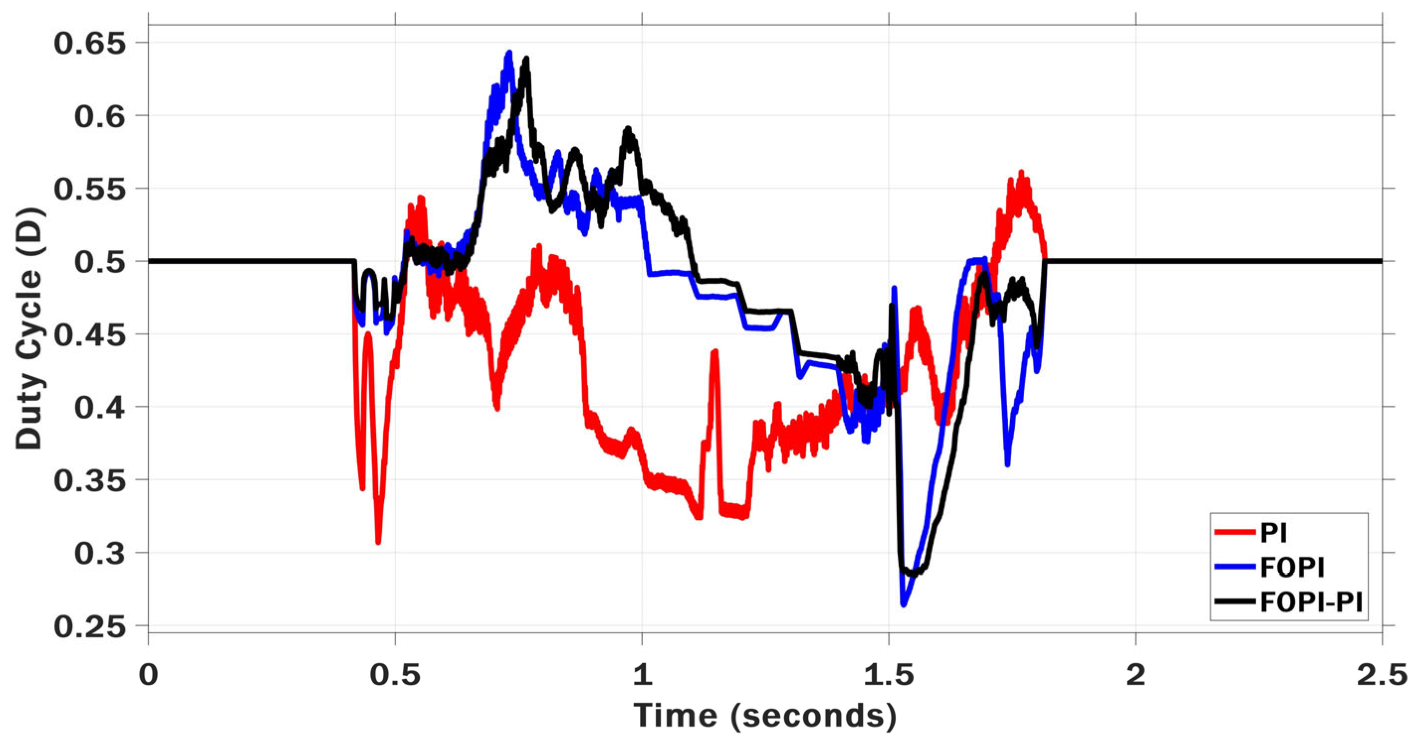
6.3. Scenario III: Realistic Irradiance Variation with Constant Temperature

In the third scenario, a true irradiance pattern with a peak of 1000 W/m² (Figure 17), recorded from Benban Solar Park in Aswan, Egypt, as observed on the first of May 2019, has been utilized. For the sake of this particular situation, the typical temperature value has been used. The duty cycle behavior for each control strategy under this scenario is depicted in Figure 18. Figure 19a,b present a comprehensive comparison of system dynamics among the RUN-based FOPI-PI, FOPI, and PI controllers for PV power and voltage, respectively. As the temperature stays constant, the PV power just follows the pattern of the irradiance. All three controllers effectively maintained power tracking during the duration of the irradiance change. The IC-MPPT-(FOPI-PI) control approach operates quickly and effectively in tracking photovoltaic power around the irradiance peak. With regard to the PV voltage, it is possible to observe, as shown in the minuscule zoomed-in picture in Figure 19b, that the FOPI-PI regulator has superior performance with a short oscillation range of 1V in comparison to the other two controllers, which have an oscillating range of 7V. Figure 19c illustrates the DC link voltage response. Figure 19d illustrates that the grid current correlates with the irradiance pattern while the temperature remains constant. Figure 19e illustrates the grid voltage.

Table 7. The IC-MPPT based PV system dynamics under the integration of the three different controllers for Scenario III.

Controller	Fitness Value (ISE)	T-Rising (Seconds)	T-Settling (Seconds)	P-Maximum (KW)	Overshoot Percentage	Efficiency %
FOPI-PI (Proposed)	326	0.0023	0.042	101.79	0.0124	99.993
FOPI	617	0.0027	0.055	101.75	0.0298	99.962
PI	694	0.0029	0.063	101.71	0.0243	99.947

summarizes the dynamic performance of the PV system under the influence of the three control methods being compared.

6.4. Scenario IV: Realistic Irradiance and Temperature Variations

In this instance, the realistic irradiance profile (Figure 17) that was utilized in the earlier scenario is implemented, in addition to the realistic temperature profile (Figure 20) that was also obtained from Benban Solar Park. The effects of the different control approaches on duty cycle performance are shown in Figure 21. A comparison of the power generated by photovoltaic cells using the FOPI-PI, FOPI, and PI control techniques is presented in Figure 22a. It has been determined that the FOPI-PI control method achieved a maximum power of 96.72 kW, with FOPI coming in second with 96.68 kW and PI coming in third with 96.47 kW. In Figure 22b, the responses of the PV voltage are shown based on the three control techniques that were tested. The FOPI-PI controller has a superior performance with a low oscillation range of 0.5 V in comparison to the other two controllers, which have an oscillation range of 5 V. As an additional point of interest, the PV voltage that is achieved by FOPI-PI is the shortest, followed by PI, and then FOPI comes in last. As shown in Figure 22c–e, the responses of the PV system to changes in temperature and irradiance are discussed. These responses include the DC link voltage, grid current, and grid voltage. The dynamic performance of the PV system, as evaluated using the three control methods, is summarized in

Table 8. The IC-MPPT-based PV system dynamics with the integration of the three different controllers for Scenario IV.

Controller	Fitness Value (ISE)	T-Rising (Seconds)	T-Settling (Seconds)	P-Maximum (KW)	Overshoot Percentage	Efficiency %
FOPI-PI (Proposed)	353	0.0024	0.042	96.72	0.0131	95.385
FOPI	667	0.0029	0.055	96.68	0.0303	95.285
PI	1023	0.0031	0.063	96.46	0.0324	95.128

.

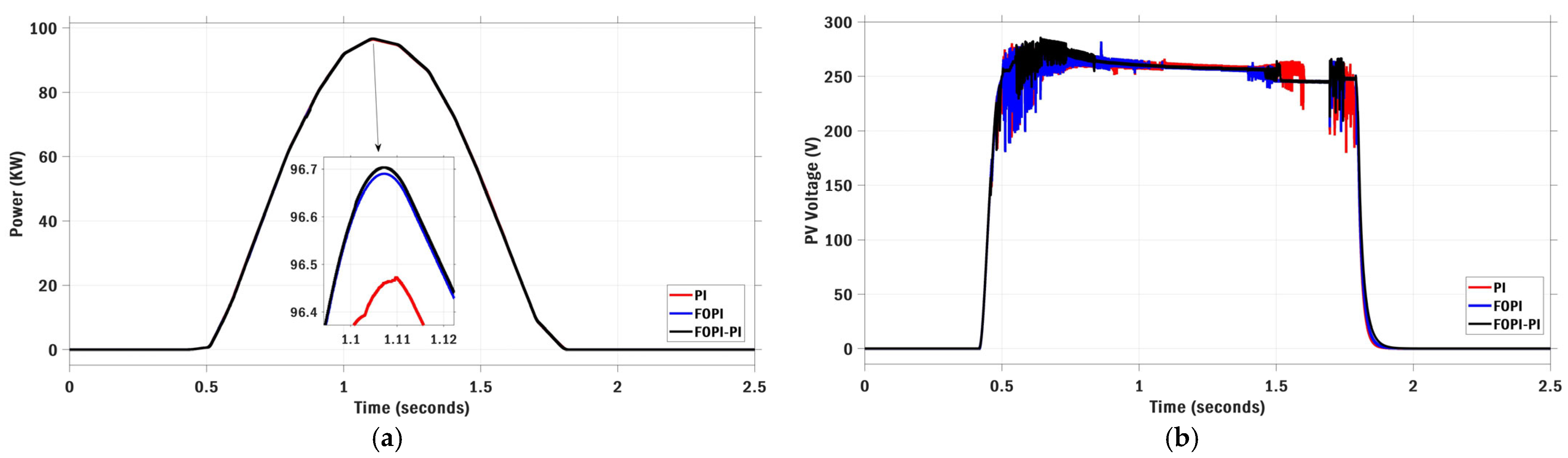
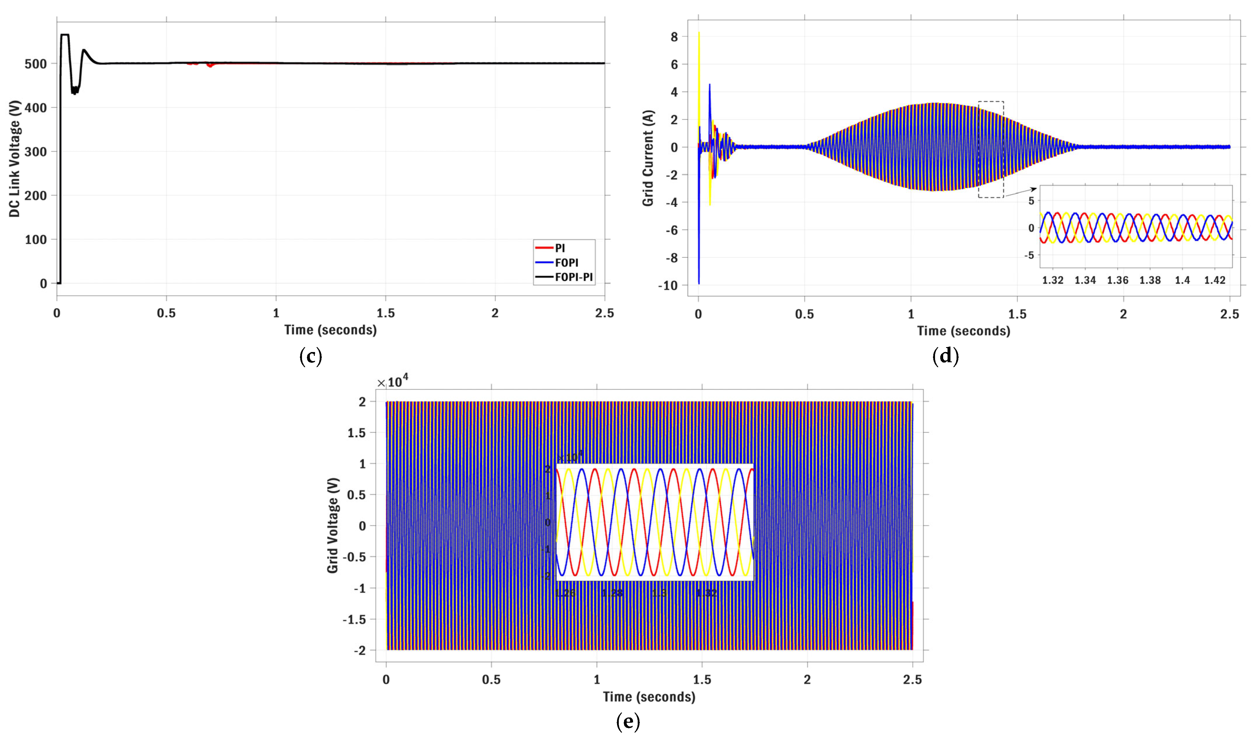
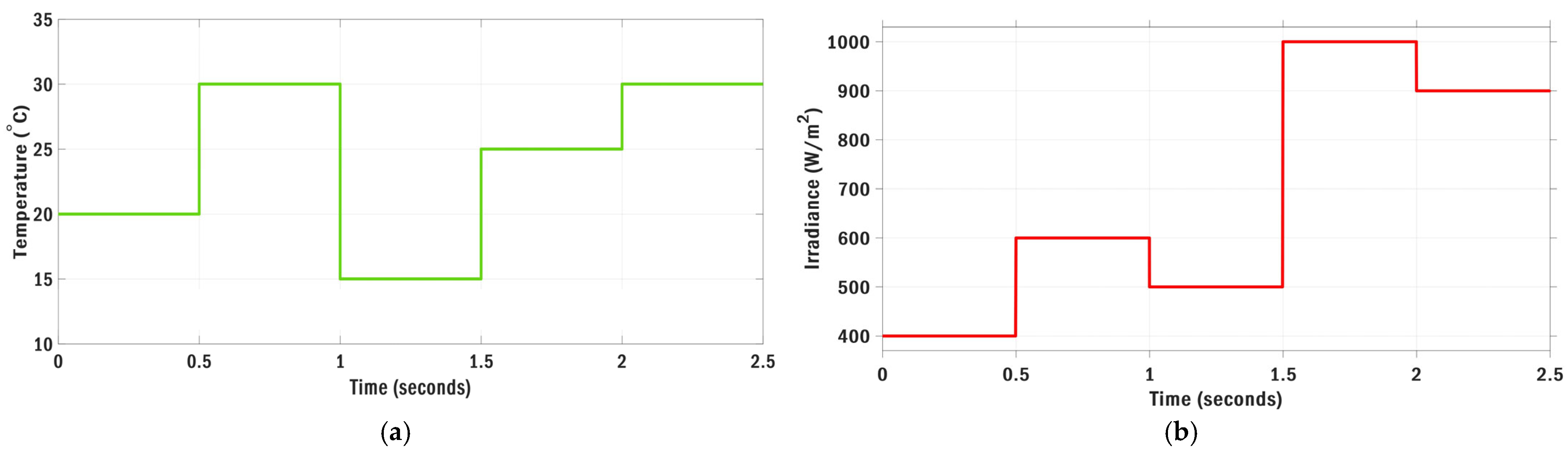
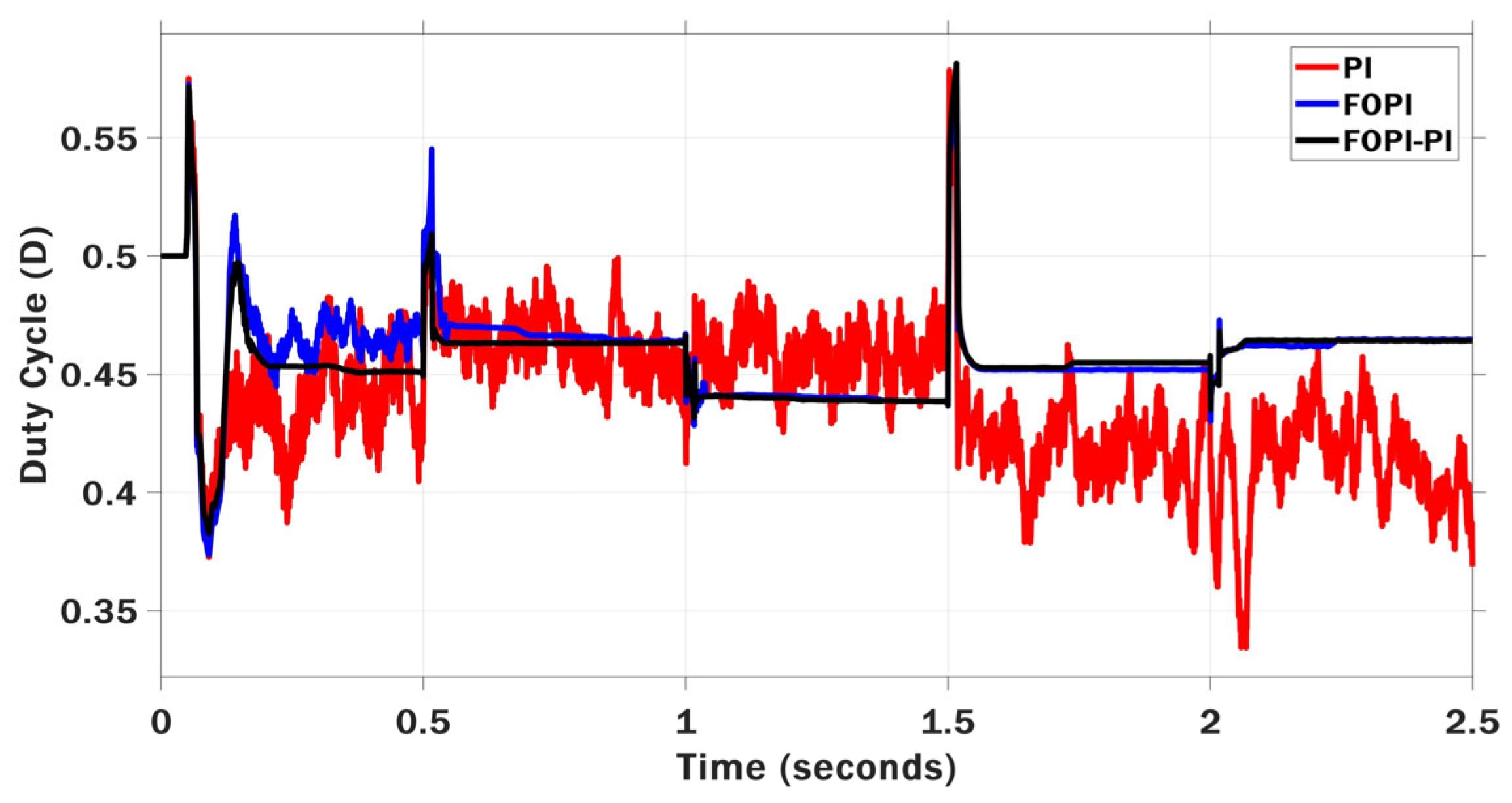
6.5. Scenario V: Multi-Stepwise Irradiance and Temperature Variations

This ultimate harsh scenario tests the resilience and efficacy of the evaluated controllers (i.e., FOPI-PI, FOPI, and PI) in response to many abrupt variations in temperature and irradiance, as illustrated in Figure 23a,b. Figure 24 displays the comparative duty cycle responses obtained using each control strategy under the given conditions. Figure 25a,b contrasts the performance of PV power and voltage, respectively, according to FOPI-PI, FOPI, and PI control techniques. All evaluated controllers efficiently track power under the impact of fluctuations in temperature and irradiance. The power response of the PV system that was obtained by FOPI-PI shows the shortest rise and settling times, followed by PI and FOPI. The tracking efficiency for MPP is notably greater in the case of IC-MPPT-(FOPI-PI), particularly during the interval from t = 1.5 to 2 s, where the FOPI-PI control strategy attains a maximum power of 100.714 KW, succeeded by 100.708 KW for FOPI, and 100.622 KW for PI. Furthermore, the FOPI-PI control approach exhibits the minimal overshoot percentage of 0.01171% and the shortest settling time of 0.02 s. Figure 25b illustrates that the PV voltage is inversely influenced by temperature, while the FOPI-PI control method exhibits the most stable PV voltage response with minimal oscillations. Figure 25c–e examine the reactions of the PV system concerning the DC link voltage, grid current, and grid voltage in relation to variations in temperature and irradiance.

Table 9. The IC-MPPT-based PV system dynamics with the integration of the three different controllers for Scenario V.

Controller	Fitness Value (ISE)	T-Rising (Seconds)	T-Settling (Seconds)	P-Maximum (KW)	Overshoot Percentage	Efficiency %
FOPI-PI (Proposed)	35.361	0.0054	0.02	100.714	0.0117	99.984
FOPI	62.149	0.0061	0.029	100.708	0.0139	99.978
PI	57.504	0.0063	0.024	100.622	0.0148	99.893

presents a comparative summary of the PV system’s dynamic performance under the three evaluated control strategies.

Finally, although this study focuses on sthe imulation-based validation of the proposed IC-MPPT-(FOPI-PI) control strategy using MATLAB/SIMULINK, it is important to assess its potential for practical deployment. The Runge-Kutta Optimizer (RUN), used in this work for controller parameter tuning, is computationally more demanding than traditional algorithms. However, the optimization process is executed offline, prior to deployment, which eliminates the need for the real-time execution of RUN on the hardware. Once the optimal controller parameters are identified, the control scheme operates as a conventional IC-MPPT-(FOPI-PI) system with fixed parameters. This design is well-suited for implementation on embedded platforms such as Digital Signal Processors (DSPs), Field Programmable Gate Arrays (FPGAs), or dSPACE systems, which are widely used in power electronics and renewable energy applications. Therefore, the computational burden at runtime is minimal, and the proposed strategy remains practically feasible for real-time control applications in grid-connected PV systems.

7. Conclusions

This study proposes an optimized MPPT control strategy for a 100 kW grid-connected PV system using the incremental conductance (IC) method. The approach integrates an FOPI controller with a conventional PI controller to enhance tracking performance, with parameters optimally tuned using the Runge–Kutta Optimizer (RUN). Simulations were conducted in MATLAB/Simulink R2024b on a benchmark 100 kW PV system connected to a medium-voltage distribution grid. The objective of optimization was to minimize the ISE. The proposed IC-MPPT-(FOPI-PI) controller was thoroughly compared against other recent metaheuristic methods, namely, AVO and GTO, as well as traditional PI- and FOPI-based MPPT controllers. Simulations were performed under five distinct climatic scenarios, including constant temperature with step changes in irradiance, gradual and realistic variations in both irradiance and temperature, and multi-step fluctuations. The results demonstrate that the RUN-based IC-MPPT-(FOPI-PI) strategy outperforms all compared methods in accurately and efficiently tracking maximum power under varying environmental conditions. For example, in the first scenario, it achieved the fastest settling time of 0.015 s—84% faster than FOPI and 82% faster than PI. It also delivered the highest maximum power output of 100.714 kW, which is 0.006% higher than FOPI and 0.092% higher than PI. In the second scenario, it reached 100.721 kW, surpassing PI by 0.006% and FOPI by 0.061%. In the third scenario, it achieved 101.79 kW at the irradiance peak, exceeding FOPI by 0.05% and PI by 0.098%. The proposed method exhibited superior performance in minimizing voltage oscillations and consistently tracked irradiance changes with minimal deviation, ensuring optimal power extraction. Overall, the RUN-based FOPI-PI controller demonstrated clear advantages in settling time, power output, overshoot reduction, and voltage stability, making it highly effective for supporting the MPPT-IC method under dynamic environmental conditions.

8. Limitations and Future Works

Despite the promising results, several drawbacks of our study may hinder the efficacy of the suggested IC-MPPT-(FOPI-PI) technique. While the proposed RUN-based IC-MPPT-(FOPI-PI) strategy is demonstrated on a 100 kW system, the control approach is scalable and can be adapted to systems of varying capacities. However, as system size increases, challenges such as dynamic response, power fluctuations, and grid interaction become more pronounced, which may affect the controller tuning and performance. Moreover, although the IC approach is more precise than P&O, it may still encounter difficulties with quickly varying irradiance and temperature fluctuations, resulting in delays in tracking the MPP. Furthermore, the IC method might run into obstacles in identifying the global MPP during partial shade circumstances, since it is exposed to become ensnared at local maxima. Moreover, the setting up of the FOPI-PI controller and the use of the IC approach need more complex computations than P&O, thereby increasing the processing workload, particularly in hardware implementations. Moreover, although the VSC used in the system theoretically allows operation in deloading mode to provide ancillary grid services, this functionality has not been considered. The PV system is assumed to operate continuously at its MPP throughout all simulations. Consequently, the potential benefits and challenges associated with deloading or grid support operations are considered outside the scope of this work. Future research may explore integrating deloading strategies and grid support functionalities to enhance the versatility and overall performance of PV systems. Furthermore, to enhance our research, the system under study might be enhanced by using battery storage or supercapacitors. This would assist in stabilizing power fluctuations and enhancing the system’s dependability. Additionally, modifications may be implemented in the existing framework of the suggested technique to enhance MPPT performance under partial shade conditions. The optimization of a grid-connected inverter may assist in diminishing the harmonics in the grid voltage and current. Moreover, substituting the FOPI-PI controller with an adaptive controller, such as a fuzzy logic controller (FLC) or a neural network-based controller, may enhance the management of nonlinearity and fluctuating atmospheric circumstances. Finally, implementing the suggested MPPT technique on an actual setup or real-time platform, such as dSpace or DSP, and comparing its performance with simulation findings would significantly validate and demonstrate the usefulness of our work.

References

1. Ahmad, R.; Murtaza, A.F.; Sher, H.A. Power tracking techniques for efficient operation of photovoltaic array in solar applications—A review. Renew. Sustain. Energy Rev. 2019, 101, 82–102. [Google Scholar] [CrossRef]
2. International Renewable Energy Agency (IRENA). Renewable Capacity Highlights; 11 April 2022; IRENA: Abu Dhabi, United Arab Emirates, 2022. [Google Scholar]
3. Yang, B.; Yu, T.; Zhang, X.; Li, H.; Shu, H.; Sang, Y.; Jiang, L. Dynamic leader-based collective intelligence for maximum power point tracking of PV systems affected by partial shading condition. Energy Convers. Manag. 2019, 179, 286–303. [Google Scholar] [CrossRef]
4. Mohamed, M.A.; Diab, A.A.; Rezk, H. Partial shading mitigation of PV systems via different meta-heuristic techniques. Renew. Energy 2019, 130, 1159–1175. [Google Scholar] [CrossRef]
5. Raiker, G.A.; Loganathan, U. Current control of boost converter for PV interface with momentum-based perturb and observe MPPT. IEEE Trans. Ind. Appl. 2021, 57, 4071–4079. [Google Scholar] [CrossRef]
6. Jately, V.; Azzopardi, B.; Joshi, J.; Sharma, A.; Arora, S. Experimental analysis of hill-climbing MPPT algorithms under low irradiance levels. Renew. Sustain. Energy Rev. 2021, 150, 111467. [Google Scholar] [CrossRef]
7. Ali, M.N.; Mahmoud, K.; Lehtonen, M.; Darwish, M.M. An efficient fuzzy-logic-based variable-step incremental conductance MPPT method for grid-connected PV systems. IEEE Access 2021, 9, 26420–26430. [Google Scholar] [CrossRef]
8. Nadeem, A.; Sher, H.A.; Murtaza, A.F. Online fractional open-circuit voltage maximum output power algorithm for photovoltaic modules. IET Renew. Power Gener. 2020, 14, 188–198. [Google Scholar] [CrossRef]
9. Nadeem, A.; Sher, H.A.; Murtaza, A.F.; Ahmed, N. Online current-sensorless estimator for PV open-circuit voltage and short-circuit current. Sol. Energy 2021, 213, 198–210. [Google Scholar] [CrossRef]
10. Fathi, M.; Parian, J.A. Intelligent MPPT for photovoltaic panels using a novel fuzzy logic and artificial neural networks based on evolutionary algorithms. Energy Rep. 2021, 7, 1338–1348. [Google Scholar] [CrossRef]
11. Dehghani, M.; Taghipour, M.; Gharehpetian, G.B.; Abedi, M. Optimized fuzzy controller for MPPT of grid-connected PV systems in rapidly changing atmospheric conditions. J. Mod. Power Syst. Clean Energy 2020, 9, 376–383. [Google Scholar] [CrossRef]
12. Chellakhi, A.; El Beid, S.; El Marghichi, M.; Bouabdalli, E.M. An amended low-cost indirect MPPT strategy with a PID controller for boosting PV system efficiency. Results Eng. 2024, 24, 103526. [Google Scholar] [CrossRef]
13. Chellakhi, A.; El Beid, S.; Abouelmahjoub, Y.; Doubabi, H. An Enhanced Incremental Conductance MPPT Approach for PV Power Optimization: A Simulation and Experimental Study. Arab. J. Sci. Eng. 2024, 49, 16045–16064. [Google Scholar] [CrossRef]
14. Chellakhi, A.; El Beid, S.; El Marghichi, M.; Bouabdalli, E.M.; Harrison, A.; Abouobaida, H. Implementation of a Low-Cost Current Perturbation-Based Improved P&O MPPT Approach Using Arduino Board for Photovoltaic Systems. e-Prime—Adv. Electr. Eng. Electron. Energy 2024, 10, 100807. [Google Scholar]
15. Mohamed Ahmed Ebrahim Mohamed, S.N.A.; Metwally, M.E. Arithmetic Optimization Algorithm Based Maximum Power Point Tracking for Grid-Connected Photovoltaic System. Sci. Rep. 2023, 13, 5961. [Google Scholar]
16. Tadj, M.; Chaib, L.; Choucha, A.; Aldaoudeyeh, A.-M.; Fathy, A.; Rezk, H.; Louzazni, M.; El-Fergany, A. Enhanced MPPT-Based Fractional-Order PID for PV Systems Using Aquila Optimizer. Math. Comput. Appl. 2023, 28, 99. [Google Scholar] [CrossRef]
17. Mansoor, M.; Mirza, A.F.; Ling, Q. Harris hawk optimization-based MPPT control for PV systems under partial shading conditions. J. Clean. Prod. 2020, 274, 122857. [Google Scholar] [CrossRef]
18. Pilakkat, D.; Kanthalakshmi, S. An improved P&O algorithm integrated with artificial bee colony for photovoltaic systems under partial shading conditions. Sol. Energy 2019, 178, 37–47. [Google Scholar]
19. Guo, K.; Cui, L.; Mao, M.; Zhou, L.; Zhang, Q. An improved gray wolf optimizer MPPT algorithm for PV system with BFBIC converter under partial shading. IEEE Access 2020, 8, 103476–103490. [Google Scholar] [CrossRef]
20. Huang, Y.P.; Huang, M.Y.; Ye, C.E. A fusion firefly algorithm with simplified propagation for photovoltaic MPPT under partial shading conditions. IEEE Trans. Sustain. Energy 2020, 11, 2641–2652. [Google Scholar] [CrossRef]
21. Fares, D.; Fathi, M.; Shams, I.; Mekhilef, S. A novel global MPPT technique based on squirrel search algorithm for PV module under partial shading conditions. Energy Convers. Manag. 2021, 230, 113773. [Google Scholar] [CrossRef]
22. Phanden, R.K.; Sharma, L.; Chhabra, J.; Demir, H.İ. A novel modified ant colony optimization-based maximum power point tracking controller for photovoltaic systems. Mater. Today Proc. 2021, 38, 89–93. [Google Scholar] [CrossRef]
23. Mosaad, M.I.; Abed El-Raouf, M.O.; Al-Ahmar, M.A.; Banakher, F.A. Maximum power point tracking of PV system based on cuckoo search algorithm—Review and comparison. Energy Procedia 2019, 162, 117–126. [Google Scholar] [CrossRef]
24. Charin, C.; Ishak, D.; Zainuri, M.A.A.M.; Ismail, B.; Jamil, M.K.M. A hybrid of bio-inspired algorithm based on Levy flight and particle swarm optimizations for photovoltaic system under partial shading conditions. Sol. Energy 2021, 217, 1–14. [Google Scholar] [CrossRef]
25. Kumar, K.K.; Bhaskar, R.; Koti, H. Implementation of MPPT algorithm for solar photovoltaic cell by comparing short-circuit method and incremental conductance method. Procedia Technol. 2014, 12, 705–715. [Google Scholar] [CrossRef]
26. Zakzouk, N.E.; Elsaharty, M.A.; Abdelsalam, A.K.; Helal, A.A.; Williams, B.W. Improved performance low-cost incremental conductance PV MPPT technique. IET Renew. Power Gener. 2016, 10, 561–568. [Google Scholar] [CrossRef]
27. Başoğlu, M.E.; Çakır, B. An improved incremental conductance-based MPPT approach for PV modules. Turk. J. Electr. Eng. Comput. Sci. 2015, 23, 1687–1697. [Google Scholar] [CrossRef]
28. Alrajoubi, H.; Oncu, S. A golden section search assisted incremental conductance MPPT control for PV-fed water pump. Int. J. Renew. Energy Res. 2022, 12, 1628–1636. [Google Scholar]
29. Stephen, A.A.; Musasa, K.; Davidson, I.E. Modelling of solar PV under varying condition with an improved incremental conductance and integral regulator. Energies 2022, 15, 2405. [Google Scholar] [CrossRef]
30. Banu, I.V.; Beniuga, R.; Istrate, M. Comparative analysis of the perturb-and-observe and incremental conductance MPPT methods. In Proceedings of the 2013 8th International Symposium on Advanced Topics in Electrical Engineering (ATEE), București, Romania, 23–26 May 2013; pp. 1–6. [Google Scholar]
31. Singh, P.; Shukla, N.; Gaur, P. Modified variable step incremental-conductance MPPT technique for photovoltaic system. Int. J. Inf. Technol. 2021, 13, 2483–2490. [Google Scholar] [CrossRef]
32. Liu, F.; Duan, S.; Liu, F.; Liu, B.; Kang, Y. A variable step size INC MPPT method for PV systems. IEEE Trans. Ind. Electron. 2008, 55, 2622–2628. [Google Scholar]
33. Gupta, A.K.; Pachauri, R.K.; Maity, T.; Chauhan, Y.K.; Mahela, O.P.; Khan, B.; Gupta, P.K. Effect of various incremental conductance MPPT methods on the charging of battery load fed by solar panel. IEEE Access 2021, 9, 90977–90988. [Google Scholar] [CrossRef]
34. Loukriz, A.; Haddadi, M.; Messalti, S. Simulation and experimental design of a new advanced variable step size incremental conductance MPPT algorithm for PV systems. ISA Trans. 2016, 62, 30–38. [Google Scholar] [CrossRef] [PubMed]
35. Oshaba, A.S.; Ali, E.S.; Abd Elazim, S.M. PI controller design for MPPT of photovoltaic system supplying SRM via BAT search algorithm. Neural Comput. Appl. 2017, 28, 651–667. [Google Scholar] [CrossRef]
36. Mirza, A.F.; Mansoor, M.; Ling, Q.; Khan, M.I.; Aldossary, O.M. Advanced variable step size incremental conductance MPPT for a standalone PV system utilizing a GA-tuned PID controller. Energies 2020, 13, 4153. [Google Scholar] [CrossRef]
37. Youssef, A.; Telbany, M.E.; Zekry, A. Reconfigurable generic FPGA implementation of fuzzy logic controller for MPPT of PV systems. Renew. Sustain. Energy Rev. 2018, 82, 1313–1319. [Google Scholar] [CrossRef]
38. Maissa, F.; Barambones, O.; Lassad, S.; Fleh, A. A robust MPP tracker based on sliding mode control for a photovoltaic-based pumping system. Int. J. Autom. Comput. 2017, 14, 489–500. [Google Scholar] [CrossRef]
39. Mao, M.; Guo, K.; Cui, L.; Zhou, L.; Zhang, Q. Classification and summarization of solar photovoltaic MPPT techniques: A review based on traditional and intelligent control strategies. Energy Rep. 2020, 6, 1312–1327. [Google Scholar] [CrossRef]
40. Kiran, S.R.; Basha, C.H.H.; Singh, V.P.; Dhanamjayulu, C.; Prusty, B.R.; Khan, B. Reduced simulative performance analysis of variable step size ANN-based MPPT techniques for partially shaded solar PV systems. IEEE Access 2022, 10, 48875–48889. [Google Scholar] [CrossRef]
41. Qais, M.H.; Hasanien, H.M.; Alghuwainem, S. A grey wolf optimizer for optimum parameters of multiple PI controllers of a grid-connected PMSG driven by variable speed wind turbine. IEEE Access 2018, 6, 44120–44128. [Google Scholar] [CrossRef]
42. Aguilar, M.E.B.; Coury, D.V.; Machado, F.R.; Reginatto, R.T. Tuning of DFIG wind turbine controllers with voltage regulation subjected to electrical faults using a PSO algorithm. J. Control Autom. Electr. Syst. 2021, 32, 1417–1428. [Google Scholar] [CrossRef]
43. Qais, M.H.; Hasanien, H.M.; Alghuwainem, S. Augmented grey wolf optimizer for grid-connected PMSG-based wind energy conversion systems. Appl. Soft Comput. 2018, 69, 504–515. [Google Scholar] [CrossRef]
44. Ebrahim, M.A.; Fattah, R.M.A.; Saied, E.M.; Maksoud, S.M.A.; Khashab, H.E. An islanded microgrid droop control using Henry gas solubility optimization. Int. J. Innov. Technol. Explor. Eng. 2021, 10, 43–48. [Google Scholar] [CrossRef]
45. Amin, M.N.; Soliman, M.A.; Hasanien, H.M.; Abdelaziz, A.Y. Grasshopper optimization algorithm-based PI controller scheme for performance enhancement of a grid-connected wind generator. J. Control Autom. Electr. Syst. 2020, 31, 393–401. [Google Scholar] [CrossRef]
46. Lotfy Haridy, A.; Ali Mohamed Abdelbasset, A.A.; Mohamed Hemeida, A.; Mohamed Ali Mohamed, Z. Optimum controller design using the ant lion optimizer for PMSG driven by wind energy. J. Electr. Eng. Technol. 2021, 16, 367–380. [Google Scholar] [CrossRef]
47. El-Banna, M.H.; Hammad, M.R.; Megahed, A.I.; AboRas, K.M.; Alkuhayli, A.; Gowtham, N. On-grid optimal MPPT for fine-tuned inverter-based PV system using golf optimizer considering partial shading effect. Alex. Eng. J. 2024, 103, 180–196. [Google Scholar] [CrossRef]
48. Mosaad, M.I. Application of DPC to improve the integration of DFIG into wind energy conversion systems using FOPI controller. Wind Eng. 2025, 49, 123–138. [Google Scholar] [CrossRef]
49. Khairalla, A.G.; Kotb, H.; AboRas, K.M.; Ragab, M.; ElRefaie, H.B.; Ghadi, Y.Y.; Yousef, A. Enhanced control strategy and energy management for a photovoltaic system with hybrid energy storage based on self-adaptive bonobo optimization. Front. Energy Res. 2023, 11, 1283348. [Google Scholar] [CrossRef]
50. Alharbi, M.; Ragab, M.; AboRas, K.M.; Kotb, H.; Dashtdar, M.; Shouran, M.; Elgamli, E. Innovative AVR-LFC design for a multi-area power system using hybrid fractional-order PI and PIDD2 controllers based on dandelion optimizer. Mathematics 2023, 11, 1387. [Google Scholar] [CrossRef]
51. Okba, S.; Saadi, R.; Hammoudi, M.Y.; Himeur, Y.; Betka, A.; Atalla, S.; Mansoor, W. Dual loop FOPI controller-based Equilibrium Optimizer tuning approach for three-phase interleaved boost converter; PEMFC HEVs. IEEE Access 2024, 12, 56789–56805. [Google Scholar] [CrossRef]
52. Shaban, H.; Houssein, E.H.; Pérez-Cisneros, M.; Oliva, D.; Hassan, A.Y.; Ismaeel, A.A.; AbdElminaam, D.S.; Deb, S.; Said, M. Identification of parameters in photovoltaic models through a Runge–Kutta optimizer. Mathematics 2021, 9, 2313. [Google Scholar] [CrossRef]
53. Ekinci, S.; Rizk-Allah, R.M.; Izci, D.; Çelik, E. Multi-strategy improved Runge–Kutta optimizer and its promise to estimate the model parameters of solar photovoltaic modules. Heliyon 2024, 10, e15332. [Google Scholar] [CrossRef] [PubMed]
54. Sajid, I.; Sarwar, A.; Tariq, M.; Bakhsh, F.I.; Hussan, M.R.; Ahmad, S.; Mohamed, A.S.N.; Ahmad, A. Runge–Kutta optimization-based selective harmonic elimination in an H-bridge multilevel inverter. IET Power Electron. 2023, 16, 1849–1865. [Google Scholar] [CrossRef]
55. Selim, A.; Kamel, S.; Houssein, E.H.; Jurado, F.; Hashim, F.A. A modified Runge–Kutta optimization for optimal photovoltaic and battery storage allocation under uncertainty and load variation. Soft Comput. 2024, 28, 10369–10389. [Google Scholar] [CrossRef]
56. Nyandieka, O.M.; Segera, D.R. A Chaotic Multi-Objective Runge–Kutta Optimization Algorithm for Optimized Circuit Design. Math. Probl. Eng. 2023, 2023, 6691214. [Google Scholar] [CrossRef]
57. Ahmadianfar, I.; Halder, B.; Heddam, S.; Goliatt, L.; Tan, M.L.; Sa’adi, Z.; Al-Khafaji, Z.; Homod, R.Z.; Rashid, T.A.; Yaseen, Z.M. An enhanced multi-operator Runge–Kutta algorithm for optimizing complex water engineering problems. Sustainability 2023, 15, 1825. [Google Scholar] [CrossRef]
58. Ahmadianfar, I.; Heidari, A.A.; Gandomi, A.H.; Chu, X.; Chen, H. RUN beyond the metaphor: An efficient optimization algorithm based on Runge–Kutta method. Expert Syst. Appl. 2021, 181, 115079. [Google Scholar] [CrossRef]
59. Bataineh, K. Improved hybrid algorithms-based MPPT algorithm for PV system operating under severe weather conditions. IET Power Electron. 2019, 12, 703–711. [Google Scholar] [CrossRef]
60. Elgendy, M.A.; Zahawi, B.; Atkinson, D.J. Assessment of the incremental conductance maximum power point tracking algorithm. IEEE Trans. Sustain. Energy 2013, 4, 108–117. [Google Scholar] [CrossRef]
61. Abdollahzadeh, B.; Soleimanian Gharehchopogh, F.; Mirjalili, S. Artificial gorilla troops optimizer: A new nature-inspired meta-heuristic algorithm for global optimization problems. Int. J. Intell. Syst. 2021, 36, 5887–5958. [Google Scholar] [CrossRef]
62. Abdollahzadeh, B.; Gharehchopogh, F.S.; Mirjalili, S. African vultures optimization algorithm: A new nature-inspired metaheuristic algorithm for global optimization problems. Comput. Ind. Eng. 2021, 158, 107408. [Google Scholar] [CrossRef]
63. Ismaeel, A.A.K.; Houssein, E.H.; Oliva, D.; Said, M. Gradient-based optimizer for parameter extraction in photovoltaic models. IEEE Access 2021, 9, 13403–13416. [Google Scholar] [CrossRef]
64. Mehta, H.K.; Warke, H.; Kukadiya, K.; Panchal, A.K. Accurate expressions for single-diode-model solar cell parameterization. IEEE J. Photovolt. 2019, 9, 803–810. [Google Scholar] [CrossRef]
65. Ali, A.I.M.; Sayed, M.A.; Mohamed, E.E.M. Modified efficient perturb and observe maximum power point tracking technique for grid-tied PV system. Int. J. Electr. Power Energy Syst. 2018, 99, 192–202. [Google Scholar] [CrossRef]
66. MathWorks. Detailed Model of a 100 kW Grid-Connected PV Array. Available online: https://www.mathworks.com/help/sps/ug/detailed-model-of-a-100-kw-grid-connected-pv-array.html (accessed on 16 April 2025).
Figure 1. The SDM of PV cell.
Sustainability 17 05841 g001
Figure 2. The studied PV system’s characteristic curves (I–V and P–V) considering numerous irradiance values at (a) 25   ° C and (b) 50   ° C .
Sustainability 17 05841 g002
Figure 3. The studied on-grid PV system.
Sustainability 17 05841 g003
Figure 4. IC-MPPT mechanism integrated with FOPI-PI controller.
Sustainability 17 05841 g004
Figure 5. FOPI-PI controller design.
Sustainability 17 05841 g005
Figure 6. Updating the positions’ mechanism according to the RK method.
Sustainability 17 05841 g006
Figure 7. The RUN searching procedure.
Sustainability 17 05841 g007
Figure 8. RUN pseudocode.
Sustainability 17 05841 g008
Figure 9. Graphical representation of the RUN optimization procedure.
Sustainability 17 05841 g009
Figure 10. The best score obtained from RUN, AVO and GTO.
Sustainability 17 05841 g010
Figure 11. Stepwise irradiance variation for Scenario I.
Sustainability 17 05841 g011
Figure 12. The duty cycle applied to the DC-DC converter using different control schemes for Scenario I.
Sustainability 17 05841 g012
Figure 13. The PV system performance under the impact of Scenario I: (a) photovoltaic power, (b) photovoltaic voltage, (c) DC link voltage, (d) utility current, (e) utility voltage.
Sustainability 17 05841 g013aSustainability 17 05841 g013b
Figure 14. The climatic variation profile for Scenario II: (a) temperature profile, (b) irradiance profile.
Sustainability 17 05841 g014
Figure 15. The duty cycle applied to the DC-DC converter using different control schemes for Scenario II.
Sustainability 17 05841 g015
Figure 16. The PV system’s performance under the impact of Scenario II: (a) photovoltaic power, (b) photovoltaic voltage, (c) DC link voltage, (d) utility current, (e) utility voltage.
Sustainability 17 05841 g016aSustainability 17 05841 g016b
Figure 17. Realistic irradiance variation for Scenario III.
Sustainability 17 05841 g017
Figure 18. The duty cycle applied to the DC-DC converter using different control schemes for Scenario III.
Sustainability 17 05841 g018
Figure 19. The PV system performance under the impact of Scenario III: (a) photovoltaic power, (b) photovoltaic voltage, (c) DC link voltage, (d) utility current, (e) utility voltage.
Sustainability 17 05841 g019aSustainability 17 05841 g019b
Figure 20. Realistic temperature profile for Scenario IV.
Sustainability 17 05841 g020
Figure 21. The duty cycle applied to the DC-DC converter using different control schemes for Scenario IV.
Sustainability 17 05841 g021
Figure 22. The PV system’s performance under the impact of Scenario IV: (a) photovoltaic power, (b) photovoltaic voltage, (c) DC link voltage, (d) utility current, (e) utility voltage.
Sustainability 17 05841 g022aSustainability 17 05841 g022b
Figure 23. The climatic variation profile for Scenario V: (a) temperature profile, (b) irradiance profile.
Sustainability 17 05841 g023
Figure 24. The duty cycle applied to the DC-DC converter using different control schemes for Scenario V.
Sustainability 17 05841 g024
Figure 25. The PV system’s performance under the impact of Scenario V: (a) photovoltaic power, (b) photovoltaic voltage, (c) DC link voltage, (d) utility current, (e) utility voltage.
Sustainability 17 05841 g025aSustainability 17 05841 g025b