Article

Impact of Urban Greenspace Pattern Dynamics on Plant Diversity: A Case Study in Yangzhou, China

1
Nanjing Institute of Environmental Sciences, Ministry of Ecology and Environment, Nanjing 210042, China
2
Co-Innovation Center for Sustainable Forestry in Southern China, Key Laboratory of Soil and Water Conservation and Ecological Restoration of Jiangsu Province, Nanjing Forestry University, Nanjing 210037, China
*
Author to whom correspondence should be addressed.
Sustainability 2025, 17(12), 5416; https://doi.org/10.3390/su17125416
Submission received: 8 May 2025 / Revised: 5 June 2025 / Accepted: 6 June 2025 / Published: 12 June 2025
(This article belongs to the Section Sustainability, Biodiversity and Conservation)

Abstract

Accelerating urbanization leads to the scarcity and fragmentation of greenspaces. Keeping biodiversity alive, i.e., enhancing greenspaces’ impacts on plant diversity in and around urban areas, is essential. This study evaluated greenspace patterns (GSPs) using landscape metrics, and calculated plant α- and β-diversity using field surveys. Bivariate correlation analysis was used to analyze the correlations among plant α- and β-diversity and landscape metrics from 2009 to 2022. Significant models were selected using stepwise regression analysis and verified by comparing fitted and field values. The results indicate that α-diversity was primarily influenced by the number of patches, wetland landscape shape index and patch richness density, imperviousness of surfaces, and forest and grassland at the 100–1000 m scale. The correlation between GSPs and α-diversity weakened with an increase in scale. Current patch richness density, Shannon’s diversity index, Shannon’s evenness index, and percentage of impervious surface and wetland significantly influenced β-diversity at the 100–300 m scale. By contrast, β-diversity was influenced by greenspace patterns at the 300–1000 m scale. There was an observed positive correlation between GSPGSPs and β-diversity that strengthened as the scale increased. These findings highlight the scale-dependent legacy effects of GSPs on plant diversity, primarily driven by the landscape pattern characteristics of urban greenspaces and the diversity of plant groups. Therefore, prioritizing the protection of large green patches and establishing designated protected areas or points for on-site conservation are crucial strategies for urban plant diversity conservation.

1. Introduction

Cities play a central role in achieving key biodiversity and sustainable development goals [1]. When looking at cities today, one of the core questions worldwide is how to keep biodiversity alive in and around urban areas and available for future generations [2]. Cities are at the heart of our economies and societies, generating over 80% of global GDP and containing 56% of the global population. However, with the majority of future urban expansion forecast to occur in the world’s most biodiverse regions, 44% of global GDP from cities is estimated to be at risk of disruption from the loss of natural habitats [3]. Moreover, Anne Larigauderie, Executive Secretary of the IPBES (Intergovernmental Science-Policy Platform on Biodiversity and Ecosystem Services), has reported that the loss of biodiversity has affected people’s access to many benefits from nature. Urban greenspaces represent an ark for urban biodiversity [4] and can have positive impacts on quality of life, human health, and wellbeing [5]. Urbanization is one of the most important global change processes [1]. Rapid urbanization often covers large areas of natural or semi-natural habitats with impervious surfaces, and the remnants of natural habitats become disconnected and fragmented, which could result in decreased urban biodiversity [6]. Increasing evidence indicates that cities can support endemic native species and others of conservation concern both at regional and global scales [7,8]. These species’ diversity in cities relies on the size, quantity, and quality of urban greenspaces [9]. Greenspaces are ecological spaces, encompassing areas dedicated to environmental protection and ecosystem services, which include both greenspace systems within urbanized regions and urban ecological spaces extending beyond these developed areas [10,11]. Greenspaces for biodiversity conservation are at the frontier of urban biodiversity research. For instance, the ecological function of greenspaces has been discussed in relation to a research framework based on landscape and metapopulation ecology [12] and the biodiversity-based theory of urban greenspace plant communities [13], as well as conservation strategies based on the origin of urban greenspaces [14]. Nevertheless, as urban areas expand, we still have a limited understanding of their ecology and how they function to conserve urban biodiversity at landscape scales [12]. Given this limited view, we explored the impact and scale effects of greenspace pattern dynamics on plant diversity so as to advance the ecology of urban greenspaces for biodiversity conservation.
Many studies on land use change, human activities, natural disturbances, and their legacy effects have been carried out during recent decades. For instance, current plant diversity has been influenced by changes in landscape patterns in sandy land over the previous 2–4 years [15]. The taxonomic diversity of plant communities in road–field boundaries has a time-lagged response to landscape changes [16]. Moreover, the legacy of historical land use in agricultural, urban, and suburban areas affects ecosystem structure, function, and biological populations, which could further affect ecosystem services [17,18]. In addition, historical land use legacy, rather than topography, soil characteristics, climate change, and current management strategies, has driven recent changes in vegetation distribution [19,20]. For example, soil compaction in forests caused by heavy livestock grazing can last for over 30 years and inhibit plant growth and seedling establishment [21]. Aber et al. [22] predicted that forest harvests would cause changes in nitrogen cycling that would take more than two centuries to recover from, and the changes in phosphorous, carbon, and nitrogen caused by agricultural practices can last for centuries and greatly affect the productivity of subsequent vegetation [23]. Even historical factors (i.e., the most recent glacial maximum) significantly affect the patterns of endemic diversity [24]. Therefore, the current vegetation distribution could be regarded as a legacy of historical landscape patterns and early land use. However, there are few studies on urban greenspace legacy effects on plant diversity.
To take into account the scale of greenspace influence on plant diversity, it is likely that research at multiple spatial scales is needed. Due to environmental heterogeneity, the distribution pattern of plant diversity varies greatly across spatial scales. A lot of previous research shows that scale effects must be duly considered when employing landscape indices for effective biodiversity prediction, and caution should be exercised in extrapolating the results across spatial scales [25]. For instance, matrix quality change on a large scale (500 m) and topography environmental conditions on a small scale (125 m) are the most influential landscape context properties for species richness, suggesting the importance of their inclusion in future biodiversity studies in the Alps. The SLOSS (single large or several small) theory and predictions show opposite results at different scales in terms of species conservation. The legacy of the “SL > SS principle”, which suggests that a single or a few large habitat patches (SLs) conserve more species than several small patches (SSs), is suitable for the patch scale. However, the theory predicts SS > SL at the landscape scale [26]. In addition, the landscape pattern has a significant impact on ecological processes, such as nutrient and substance distribution; thus, plant diversity varies greatly across spatial scales [27]. Urban greenspaces are characterized by highly fragmented, small, and isolated patches of greenspace. However, much remains unknown about how large urban greenspaces need to be in order to conserve biodiversity [12]. Considering the scale effect can effectively reconcile the inherent contradiction between urban development and biodiversity conservation [28], thereby assisting in proposing conservation strategies based on urban greenspaces.
Research on the impact of urban greenspace on plant diversity is lacking. This study contributes to the research on the scale-dependent legacy effect of the impact of urban greenspace on plant α- and β-diversity at multiple spatiotemporal scales. Here, we present a comprehensive assessment of the impact and scale effect of urban greenspace pattern (GSP) dynamics on plant diversity in Guangling District, Yangzhou City. Guangling District is strategically situated at the confluence of the Beijing–Hangzhou Grand Canal and the Yangtze River in China. It serves not only as a pivotal area where the Huaihe River merges with the Yangtze River but also as a vital water source of the South-to-North Water Transfer East Route Project (Sanjiangying). Approximately 700 million cubic meters of water is annually transported to Northern China. Moreover, it boasts an exceptionally well-preserved natural habitat, making it an ideal location to explore this intricate mechanism. Specifically, this study has two specific objectives: (1) to determine the impact and scale effect of GSP dynamics on plant diversity and (2) to explore the influencing mechanism between GSP characteristics and plant α- and β-diversity.

2. Data Acquisition and Research Methods
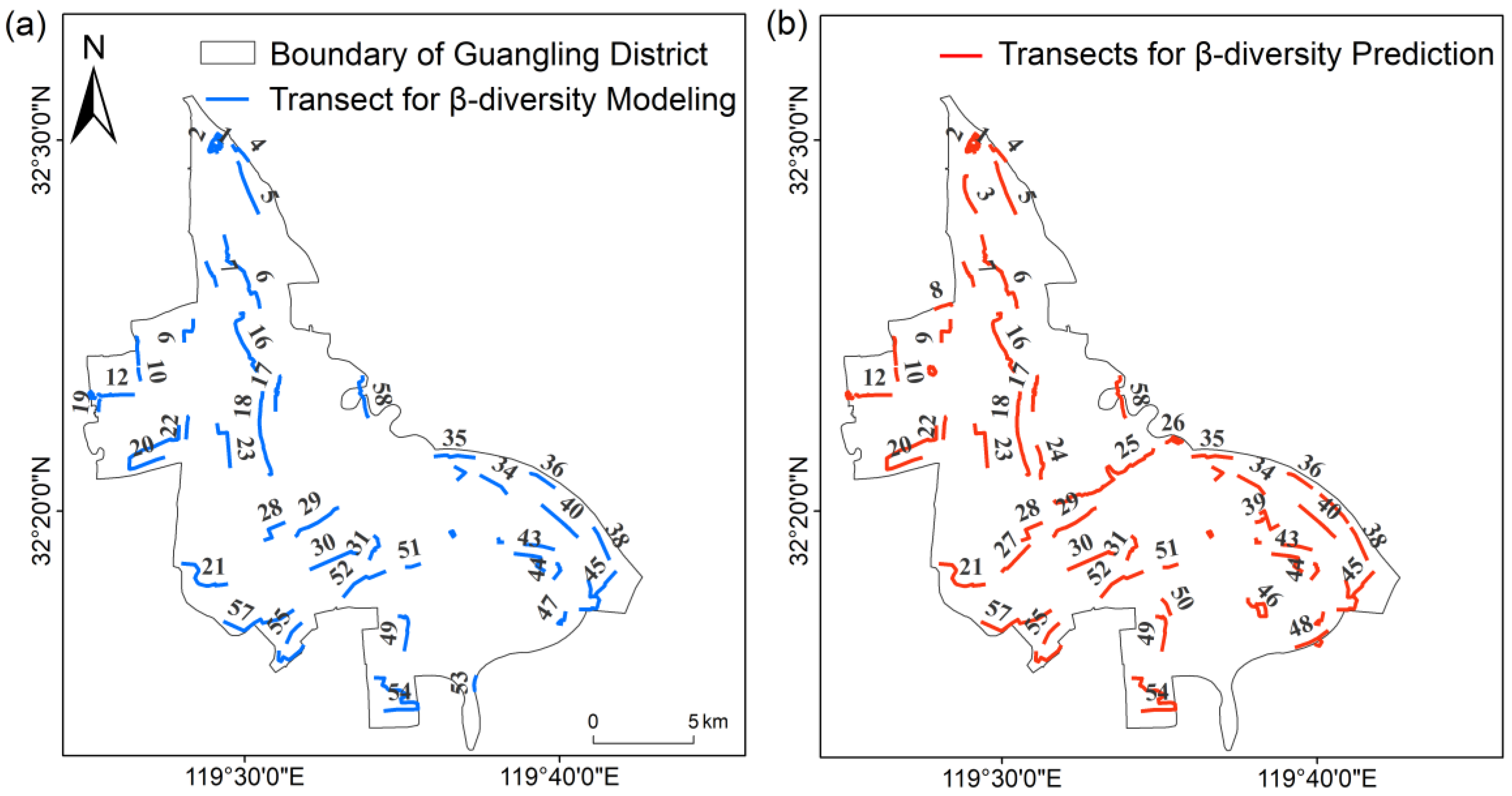
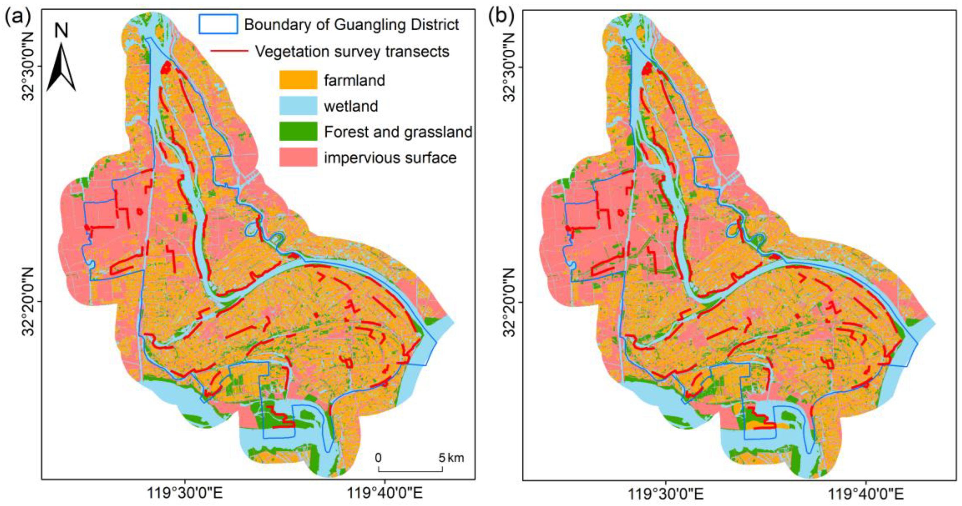
2.1. Research Area

This study was conducted in the Yangtze River Delta, Guangling District, Yangzhou City, China, which is strategically situated at the confluence of the Beijing–Hangzhou Grand Canal and the Yangtze River in China. Guangling District (119°25′–119°43′ E, 32°13′32°18′ N) covers nearly 265.36 km2 and boasts a unique topography known as the “seven rivers and eight islands”, characterized by seven distinct rivers originating from different sources and dividing the region into eight islands. This area encompasses a national wetland park and a national water conservancy scenic spot, serving as a crucial drinking water source protection area for Yangzhou City. Moreover, it preserves Yangzhou lake’s pristine ecological natural environment, featuring an exquisite plain-type wetland landscape with exceptional ecological resources and abundant biodiversity. Over the past decade, numerous projects focusing on ecological protection and restoration have been implemented, with an emphasis on establishing spatial patterns for species protection, facilitating species migration and gene exchange. Concurrently, significant changes have occurred in the GSPs. Consequently, this region presents an ideal opportunity to explore the effects of the GSPs on plant diversity.

2.2. Biodiversity Index

During field investigations, we comprehensively considered the continuity and accessibility of each transect within the same land use type while striving to cover areas with high plant diversity as extensively as possible. All vascular plant species were recorded from April to November 2022 within a plot of 25 km2 (5 km × 5 km) that was positioned in each element (Figure 1), resulting in a total of 58 vegetation survey transects (0.6–7.3 km in length) that covered greenspaces such as cropland, wetlands, forests, and built-up greenspaces (parks, roads, and riverbank green belts), with a total length of 132.59 km (Figure 2). The 58 transects were evenly spread across land use types as much as possible, and all transects from 2009 and 2022 were spatially matched to compare legacy effects.
(1) α-diversity
Species richness is considered the most important structural and functional component of biodiversity, serving as a crucial objective indicator for assessing the abundance of plant resources within a given region. α-diversity represents diversity within biological boundaries, and the calculation formula for the α-diversity of each vegetation survey transect is as follows:
R   =   S
In this formula, R is the species richness index, and S is the number of species.
(2) β-diversity
β-diversity refers to the heterogeneity among habitats, and it serves as an indicator of species segregation across different environments. In accordance with the conventional approach proposed by Whittaker [29], the calculation process is as follows:
β w   =   S / m a     1
In this formula, S is the total number of species in the plot, and ma is the number of species in each vegetation survey transect. Considering the coexistence patterns of species across multiple communities, the average pairwise dissimilarity values may not accurately reflect the overall compositional heterogeneity within a pool of more than two sites. In this study, we refrained from using the average βw index of paired transects as a representation of overall β-diversity. Instead, we randomly selected 5–13 transects in adjacent plots and calculated the overall βw values to analyze the β-diversity between different habitats (Figure 2) [30,31].

2.3. Greenspace Pattern Data

Landscape ecology provides methods and tools for assessing measures of biodiversity at multiple scales to support decision-making in urban areas and greenspaces [32]. The landscape index can effectively capture GSP information, and it serves as a robust indicator of plant diversity, making it a valuable tool for scientific inquiry. The quantization methods for GSP features encompass the complexity, fragmentation, diversity, aggregation, and separation indices, and these indices have certain limitations such as collinearity and redundancy. Therefore, after excluding the landscape index exhibiting strong collinearity, we selected the number of patches (NP), patch density (PD), edge density (ED), patch richness density (PRD), percentage of landscape (PLAND), landscape shape index (LSI), Shannon’s diversity index (SHDI), and Shannon’s evenness index (SHEI) to comprehensively assess the landscape characteristics in a more rigorous and scientifically sound manner. Simultaneously, the PLAND, NP, PD, ED, and LSI indices of cropland, wetland, forest, grassland, and impervious surface were extracted and analyzed.
In July 2009 and June 2022, data processing and spatial analyses were conducted and Landsat remote sensing data were utilized with ENVI 5.3 and ArcGIS 10.5 software. After radiation and geometric precision correction, we used the object-oriented supervised classification method to extract four types of patches in the study area, namely, farmland, wetland, forest and grassland (including forested areas and greenspaces within built-up regions), and impervious surfaces (such as constructed areas within towns, villages, and roads). The classification accuracy reached more than 90% (Figure 3). Buffer zones of different scales (with radii of 100, 200, 300, 400, 500, 600, 700, 800, 900, and 1000 m) were established around the transect line. The landscape index was computed utilizing Fragstats 4.2 software, the details of which are provided in the online help manual of Fragstats 4.2.

2.4. Statistical Analysis

A bivariate correlation analysis was conducted to examine the relationship between each landscape index and its corresponding plant diversity index. The landscape index that exhibited a significant correlation with both α- and β-diversity indices of plant species at various scales was selected for further investigation. With the plant diversity index as the response variable and the landscape index as the independent variable, the stepwise regression analysis method was used to perform stepwise regression between 46 field transversal survey data and landscape indices at different scales. In order to mitigate the spatial autocorrelation of landscape indices, it is imperative to first address multicollinearity through a variance inflation factor (VIF) analysis. We initially considered the VIF for 23 indices, including the NP, PD, ED, PRD, PLAND, LSI, SHDI, and SHEI (Table 1). At spatial scales ranging from 100 m to 1000 m, the VIT values between indicators differed. Indices with VIF > 10 were excluded. Subsequently, the optimal regression model could be identified through rigorous screening (p < 0.01). Finally, 12 landscape indices that were not utilized in the generation of pattern lines were incorporated into the optimal regression model for predicting plant diversity, and they were subsequently validated against the actual α- and β-diversity indices. The transect lines used for modeling and fitting were randomly distributed across the study area. A data analysis was conducted using the statistical software SPSS 22.0 and OriginLab Origin 2021.

3. Results

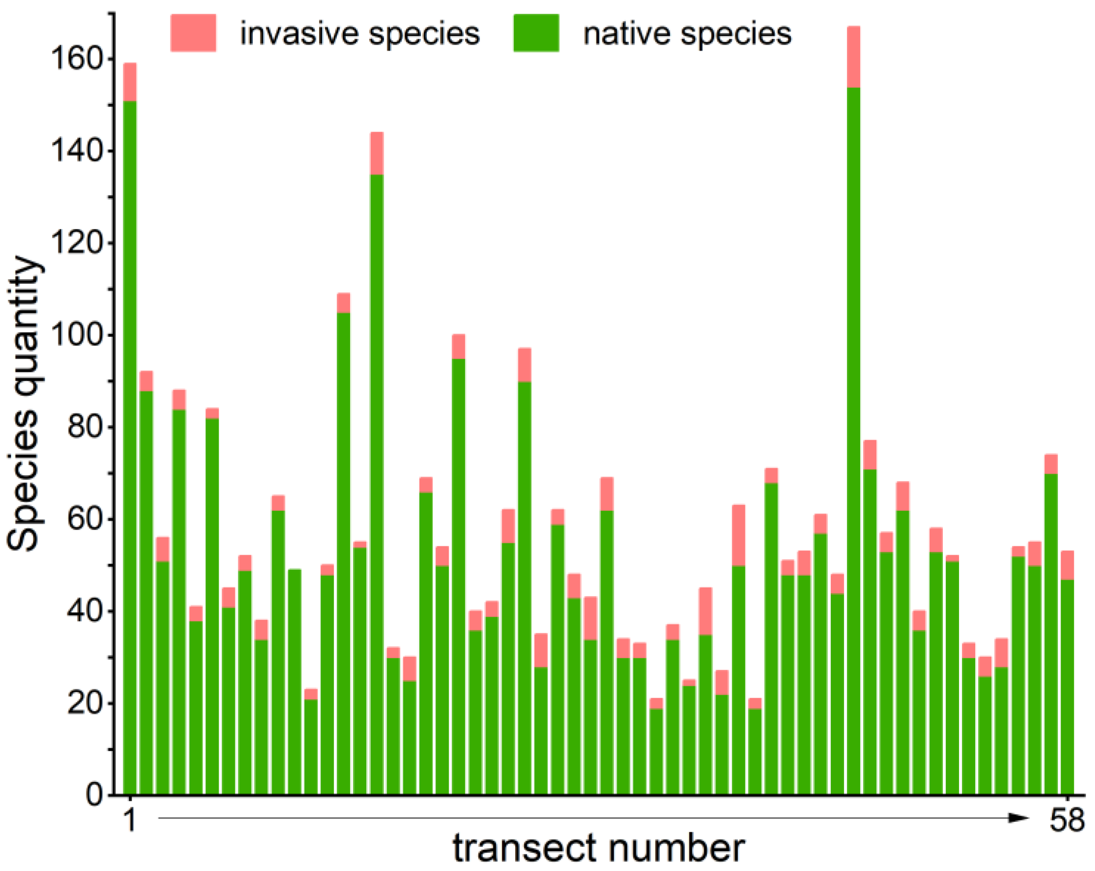
3.1. Greenspace Components and Plant Species Composition

A total of 136 families, 429 genera, and 634 plant species were identified in the surveyed region, including 29 species endemic to China (Heptapleurum arboricola, Chimonanthus praecox, Taxodium “Zhongshansha”, Actinidia chinensis, Bischofia polycarpa, etc.), 11 species in the List of National Key Protected Wild Plants (Metasequoia glyptostroboides, Cycas revoluta, Ginkgo bilob, Liriodendron chinense, etc.), and 35 alien invasive plants (Solidago canadensis, Phytolacca american, Bidens pilosa, Impatiens balsamina, etc.). The compositions of the different transects showed that the proportion of invasive species ranged from 0 to 22.22% (Figure 4). The results showed that the top 10 dominant families of wild vascular plants in Guangling District, Yangzhou City, were Gramineae (57 species), Asteraceae (56 species), Rosaceae (31 species), Fabaceae (30 species), Labiatae (21 species), Polygonaceae (18 species), Asparagaceae (16 species), Amaranthaceae (16 species), Cyperaceae (13 species), and Cucurbitaceae (13 species) (Table S1).
Cropland was primarily distributed in the southern part, while the built-up area was concentrated in the central region. Wetlands, forests, and grassland were mainly located in the northern areas, along the banks of the Beijing–Hangzhou Grand Canal and the Yangtze River (Figure 3). The variation in the city’s greenspaces from 2009 to 2022 was as follows: the cropland area decreased from 91.09 km2 to 80.51 km2, a reduction of 10.59 km2; the wetland area decreased from 60.98 km2 to 58.29 km2, a reduction of 2.69 km2; the forest and grassland area increased from 24.83 km2 to 29.13 km2, a gain of 4.30 km2; and the impervious surface area increased from 88.46 km2 to 97.44 km2, a gain of 8.97 km2. In 2009 and 2022, the urban built-up area was 60.83 km2 and 67.39 km2, respectively, with greenspace ratios of 33.4% and 42.07% (Table 2).
A vegetation survey (Table 3) showed that common native tree species (such as Citrus medica, Eriobotrya japonic, Prunus armeniaca, and Broussonetia papyrifera), various weeds (such as Cayratia japonica, Oxalis corniculate, and Setaria viridi), and invasive plants (such as Phytolacca americana, Bidens Pilosa, Solidago canadensis, and Alternanthera philoxeroides) were widely distributed in both croplands and wetland patches. In addition, a large number of horticultural plants, such as Chimonanthus camphora, Ginkgo biloba, Magnolia denudate, and Viburnum macrocephalum f. keteleeri, were planted in the urban greenspaces. Fallopia multiflora, Glechoma longituba, Spiranthes sinensis, Carex brachyathera, etc., occurred less frequently in the study area and were mainly distributed in the region known as “seven rivers and eight islands”. β-diversity refers to the heterogeneity among habitats, resulting mainly from species turnover (replacement) components. Species turnover encompasses the replacement of species along spatial or environmental gradients, thereby contributing to β-diversity. Therefore, the occurrence of these rare species increased the species composition difference among different habitats and the vegetation β-diversity in the study area.

3.2. Landscape Indices with Significant Effects on Plant Diversity

A bivariate correlation analysis showed that the landscape index had a significant influence on both α- and β-diversity (p < 0.05) (Table 4). Plant diversity was primarily influenced by the GSPs of different years and land use types, including cropland, wetland, and forest and grassland, as well as impervious surfaces. Among these factors, the NP and LSI exerted a more significant impact on plant α-diversity. Additionally, the PRD, PLAND, SHDI, and SHEI emerged as crucial determinants affecting plant β-diversity. PRD, SHDI, etc., increased the abundance and fragmentation of patch types that could provide more habitats for both rare native and invasive species. The occurrence of rare native and invasive species increased the species composition difference among different habitats and the β-diversity in the study area. The responses of α- and β-diversity to the GSPs varied significantly across different scales. Thirteen years ago, the shape index of forest and grassland exerted a significant influence on α-diversity below the 700 m scale; however, at present, it only affected α-diversity at the 100 m scale. Both in 2009 and at present, the α-diversity below the 500 m scale was predominantly influenced by the NP, particularly in wetlands, as well as in forest and grassland patches. Moreover, thirteen years ago, the PRD index exerted an influence on β-diversity at the 300–400 m scale; however, at present, it no longer exerted any impact on β-diversity. Both in the past and at present, the PLAND index significantly influenced β-diversity across all spatial scales, particularly with regard to the proportion of wetlands and impervious surface patches. Additionally, the SHDI and SHEI has started to affect β-diversity at the 400–1000 m scale.
In general, the allocation patterns of patches in greenspaces play a crucial role in influencing plant diversity, with their effects varying across temporal and spatial scales. The distribution pattern of wetland, forest, grassland, and impervious surface patches significantly influences α-diversity, while the spatial distribution of wetland and impervious surface patches primarily impacts β-diversity.

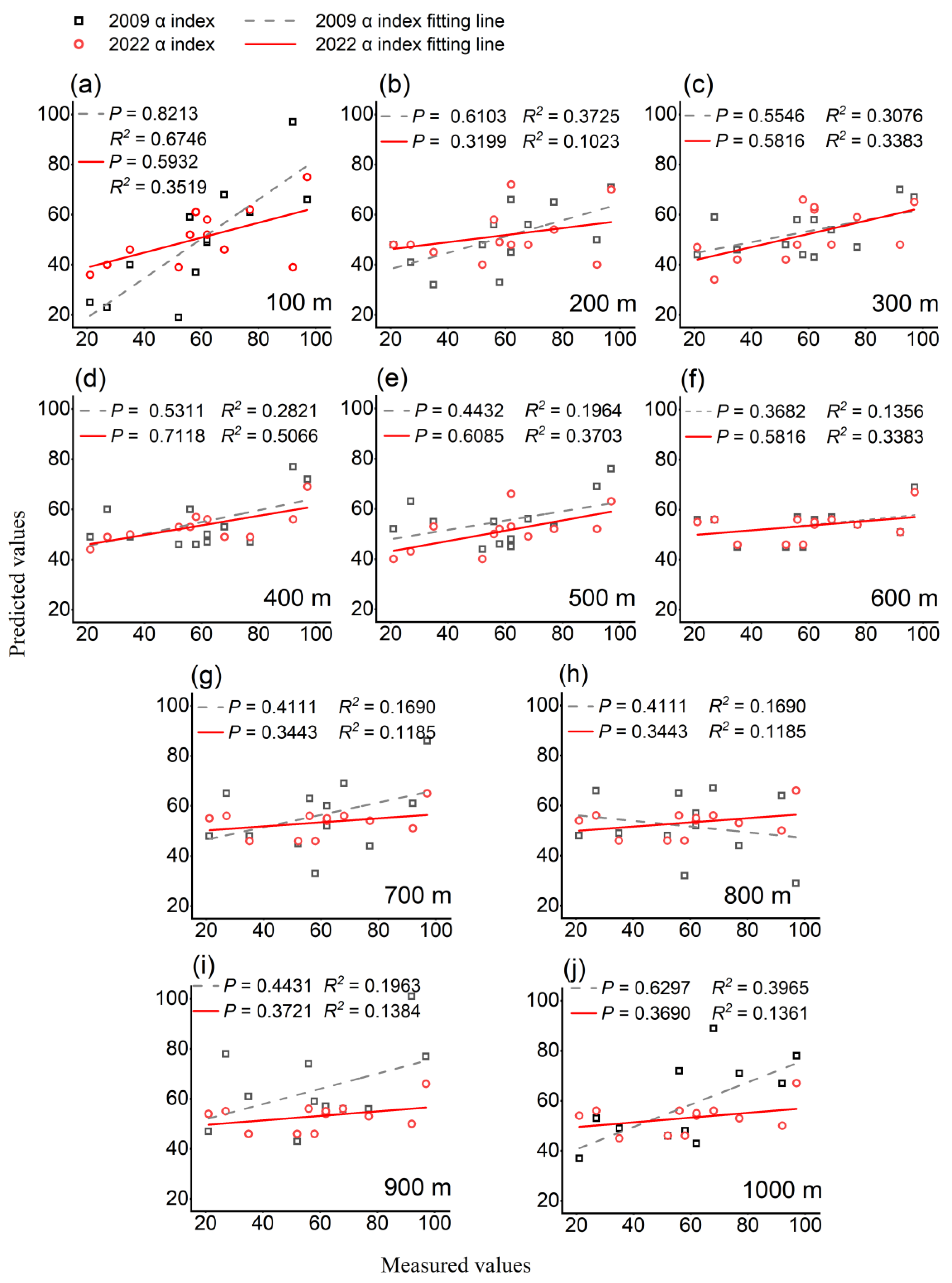
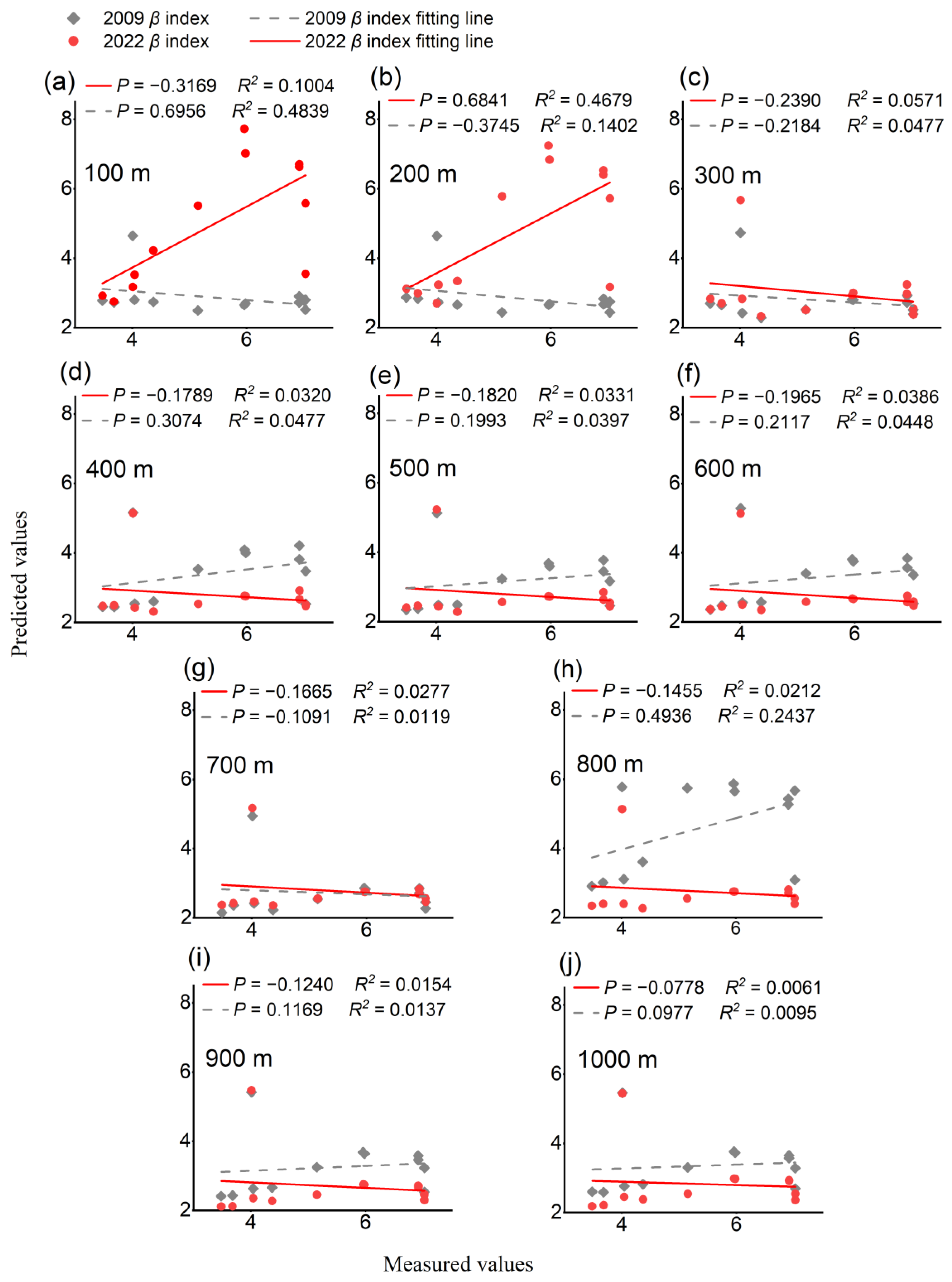
3.3. Impact of Greenspace Pattern on Plant Diversity

The results of the stepwise regression model and comparison of the fitted and field values indicate that the impact of the GSPs on plant diversity is controlled by different temporal factors (Table 5 and Figure 5 and Figure 6). At all scales, the regression model composition depicting the relationship between plant α- and β-diversity and the GSPs exhibited significant disparities. Compared with the present, the landscape index components influencing the α- and β-diversity of plants in the GSPs from 2009 were more complex. The determination coefficient (R2) of the optimal regression model and the fitted and field values exhibited discernible patterns. The present plant diversity was significantly influenced by the GSP characteristics from 2009, with this impact being strongly scale-dependent. According to the optimal regression model (Table 5), thirteen years ago, the α-diversity in the GSPs was primarily influenced by the LSI, forest and grassland patch shape index (LSIf), density index (PDf), edge density index (EDf), and impervious surface patch shape index (LSIi); moreover, β-diversity was significantly influenced by the proportion of impervious surface patches (PLANDi), as well as the shape and density indices of wetland patches (LSIw and PDw) at scales below 700 m. At scales ranging from 800 to 1000 m, the SHDI and SHEI emerged as dominant factors shaping β-diversity patterns. In the current GSPs, the pattern characteristics of forest and grassland and wetland patches (NPf, LSIf, PLANDf, and NPw) at scales below 500 m influenced α-diversity, and only patch richness density (PRD) explained α-diversity at scales between 500 and 1000 m. Below the 200 m scale, the NPi influenced β-diversity; at the 200–800 m scale, the dominance of impervious surface, forest and grassland, and wetland patches jointly influenced β-diversity; when it reached 800–1000 m, the SHEI began to mainly influence β-diversity. There were obvious differences in the determination coefficient (R2) of the optimal regression model of the relationship between plant diversity and the GSPs across various scales: (1) the coefficient of determination (R2) for β-diversity exhibited a significantly greater magnitude than that for α-diversity; (2) the coefficient of determination (R2) for the impact of the GSPs on plant diversity exhibited a higher value in 2009 than its current level; and (3) essentially, with an increasing spatial scale, the correlation between the GSPs and α-diversity diminished (R2 values gradually decreased), while the association between the GSPs and β-diversity strengthened (R2 values gradually increased). Thirteen years ago, the correlation between the GSPs and β-diversity at the 800 m scale (R2 = 0.996) exhibited a stronger association than that at 100 m (R2 = 0.721), 200 m (R2 = 0.747), 300 m (R2 = 0.853), 400 m (R2 = 0.989), 500 m (R2 = 0.984), 600 m (R2 = 0.990), 700 m (R2 = 0.991), 900 m (R2 = 0.987), and 1000 m (R2 = 0.981).
The results of the accuracy test (Figure 5 and Figure 6) indicated a significant variation in the fitting effect between the measured and predicted plant diversity values as the scale changed. The measured and predicted α-diversity values demonstrated a strong fit across scales ranging from 100 to 1000 m (Figure 5a–d,j). The significance of the fitting effect essentially decreased with an increasing scale, highlighting the particularly prominent impact of the GSPs from 2009 on α-diversity. At a scale of 100–300 m, the measured β-diversity value and the predicted regression model value had a better fitting effect at present (Figure 6a–c). Conversely, at a scale of 400–1000 m, it was evident that the GSPs dominated β-diversity thirteen years ago compared to current conditions (Figure 6d–j).
In conclusion, the temporal parameter, acting as an abiotic factor, exerted a significant influence on the distribution status of plant diversity patterns. In the Guangling District of Yangzhou, the GSPs from 2009 had a significant impact on plant α-diversity, with the LSI, NP, and PRD identified as the main influencing factors. Currently, at a scale of 300 m, the GSPs had a greater influence on plant β-diversity, while at scales ranging from 300 to 1000 m, β-diversity was primarily influenced by the GSPs from 2009. The dominant factors in this context were the SHDI, SHEI, and PLAND.

4. Discussion

4.1. Legacy and Scale Effects of Greenspace Pattern

In this study, we observed that the plant α- and β-diversity values in the study area were significantly influenced by both the present GSPs and that from 2009, with the historical GSPs exerting a particularly noteworthy impact (Table 5 and Figure 5 and Figure 6). Previous research has shown that the plant community composition and plant diversity are shaped by the initial landscape pattern and land use. For instance, the land use patterns from 2 to 4 years ago [15], 20 to 40 years ago [33], or even longer (200 years) [34] have exerted a significant influence on the current biodiversity distribution, even surpassing the impact of the present GSPs [35], which suggests a lasting legacy effect within the historical context of land use. Rapid urbanization leads to the conversion of numerous natural habitats into impervious surfaces, resulting in direct alterations to the land cover and vegetation distribution. Moreover, it significantly modifies urban hydrothermal conditions and other environmental characteristics, thereby continuously impacting the growth and development of vegetation [36]. The hydrological and soil characteristics of early land use persist even after disturbed urban areas, such as impervious surfaces or croplands, are transformed into revegetated greenspaces [37]. For example, investigations conducted on forests and grasslands have revealed that agricultural activities can lead to long-lasting alterations in soil pH, carbon, and nitrogen levels [38,39]. These changes can persist for several decades to centuries, even after the conversion of cropland back into forest or grassland, significantly impacting subsequent vegetation productivity [23]. Moreover, some effects of habitat fragmentation on soil C and N retention, productivity, pollination, and seed propagation efficiency can be delayed by up to a decade [40,41]. The effects of historical habitat fragmentation can persist even after connectivity is re-established [42]. Even in the event of natural habitat destruction, mature plants may experience a temporary disappearance; however, a species will only face local extinction if seedlings fail to thrive due to disturbances or prolonged depletion of the soil seed bank [43]. The results of this study also show that the current plant distribution pattern in the study area is a legacy of the historical greenspace pattern and early land use, aligning with numerous recent research findings [16,20,33]. Therefore, historical greenspace pattern dynamics must be considered in the study of urban plant diversity.
In this study, we also observed that the impact of the GSPs from 2009 on plant α-diversity was more pronounced within a scale of 100–1000 m, and this impact progressively diminished as the scale increased (the R2 value gradually decreased). By contrast, at a spatial scale of 300 m, the current GSPs exerted a more pronounced influence on plant β-diversity. Furthermore, within a range of 300–1000 m, β-diversity was dominated by the GSPs from 2009. This suggests that, as the spatial scale increased, there was a longer lag time in the plant β-diversity response to changes in GSP dynamics. Additionally, the impact of the GSPs on β-diversity became more prominent with an increasing scale (as indicated by the gradual increase in the R2 values) (Table 5 and Figure 5 and Figure 6). A potential explanation for this outcome lies in the spatial heterogeneity of processes such as material nutrient cycling, pollination, and seed propagation efficiency [40]. Consequently, the distribution pattern of plants is influenced by variations at different spatial scales [27]. In addition, processes such as species interactions, environmental heterogeneity resulting in resource complementation/supplementation, increased habitat diversity, or ecological drift [44] could affect extinction/colonization dynamics and moderate beta-diversity patterns across a landscape [26,45]. For example, a previous study found that, in the Gobi Desert region of Alxa, China, β-diversity has a significant linear relationship with geographic distance [46]. Moreover, a recent study conducted on the coast of the Yellow Sea, eastern China, found that the invasion of exotic cordgrass Spartina alterniflora can have long-distance effects on native species up to 10 km away, and this long-distance interaction has significantly altered the spatial distribution of plant diversity along the Yellow Sea coastline over the past four decades [47]. The plant groups investigated in the study area primarily consisted of edge species, including both annual and perennial herbs, which had high immigration and colonization efficiency. Even if there is a short-term disturbance leading to the destruction or loss of some existing vegetation, it was observed that the buffer zone with a radius of 1000 m encompasses a greater variety of greenspaces than the buffer zone with a radius of 300 m, as evidenced by data from thirteen years ago. Over time, the marginal species in the surrounding original green landscape and even some trees and shrubs will gradually spread and colonize the current area. A study on the plant species richness of road–field boundaries in central–western France suggested that the taxonomic diversity of the plant communities of road–field boundaries had a time-lagged response to landscape changes, and the impact varied across scales of 250 m, 500 m, and 1000 m [16], which is similar to the results of our study. The historical context of the GSPs in the study area had a significant impact on the distribution pattern of urban plant diversity, and this influence varied with the spatial scale, indicating that the GSPs’ significant impact on plant diversity exhibits scale-dependent legacy effects.

4.2. Differences in Green Spatial Pattern and Plant Groups

The vegetation distribution pattern in the study area was primarily influenced by historical greenspace patterns and early land use practices, and it was significantly impacted by the degree of fragmentation (including quantity, density, and edge density) and the shape, diversity, and evenness indices of impervious surfaces, as well as other various green patches, which highlights the importance of assessing urban biodiversity in conjunction with greenspace patterns. Patch size influences species extinction–colonization dynamics [26], serving as a significant determinant of plant community composition and species diversity. One of Diamond’s principles, inspired by MacArthur and Wilson’s theory of island biogeography [48], is that a larger area of greenspace can host a greater number of species, suggesting that increasing the greenspace area will benefit biodiversity conservation. Moreover, the “ecosystem decay” hypothesis suggests that ecological processes change in smaller and more isolated habitats such that more species are lost than would have been expected simply through the loss of habitat alone [49]. The aforementioned theories and hypotheses provide support for the SL > SS principle, which states that a single or a few large habitat patches (SL) conserve more species than several small patches (SSs) [26]. For example, research conducted on grassland and semi-arid sandy ecosystems has demonstrated that larger patch areas have higher plant diversity [50,51]. However, contrary to our findings, the fragmentation level of impervious surfaces and greenbelt patches in the study area exhibited a positive influence on species richness (Table 4). This discrepancy can potentially be attributed to variations in the landscape patterns and plant communities within the urban greenspace specifically located in the study area.
The urban greenspace in the study area comprised a diverse range of landscape types, including cropland, wetland, forest and grassland, and impervious surfaces, and it is characterized by its highly fragmented nature, with small and isolated greenspace patches. The island biogeography theory and “ecosystem decay” hypothesis support the SL > SS principle based on patch scale; however, landscape-scale patterns show the opposite: for sets of patches with an equal total habitat area, species richness and evenness decrease with an increasing mean size of the patches comprising that area [52], thus showing SS > SL results. In addition, the field investigation showed that the dominant families in the study area were Gramineae, Asteraceae, Rosaceae, legumes, labiaceae, polygonaceae, Aspartaceae, and Amaranthaceae, including 35 exotic invasive plants. From 2009 to 2022, the urban built-up area increased by 6.56 km2, with greenspace ratios increasing from 33.4% to 42.07%. During the period of rapid urbanization from 2009 to 2022, invasive species were more likely to colonize the revegetated greenspaces, and invasive plants appeared in 57 out of 58 transects.
The majority of species within these families exhibited marginal characteristics as either annual or perennial herbs, demonstrating remarkable immigration and colonization efficiency and being widely distributed across the landscape. A strong positive correlation was observed between plant α-diversity and both the impervious surface and greenspace shape index (Table 3 and Table 4). Greenspaces with intricate shapes exhibit greater habitat diversity and a more frequent exchange of energy and materials [53]. Predictions based on extinction–colonization dynamics show a higher per unit area immigration rate over SS than SL due to lower patch-to-patch distances in SS than SL and a higher edge-to-area ratio over SS than SL [26]. The dominant species in the urban greenspace in the study area were also characterized as edge species, exhibiting SS > SL results. This finding aligns with that of a recent study that was based on 435 landscapes across eight regions and that showed that successful agricultural measures to enhance biodiversity include diversifying cropland and reducing field size, which can multiply biodiversity while sustaining high yields in both conventional and organic systems [54].
We also found that, while numerous landscape indices were associated with plant β-diversity across various patch types, the primary driver of β-diversity was landscape diversity (the PRD, PLAND, SHEI, and SHDI), particularly the proportion of wetland and impervious surface patches (PLANDw and PLANDu) (Table 5 and Figure 5 and Figure 6). Studies of the relationship between landscape diversity and biodiversity are abundant, consistently showing that landscape heterogeneity exhibits a significantly positive correlation with species β-diversity [55], and this correlation also supports the SL > SS principle, as evidenced by the higher β-diversity index in SS patches [56]. Generally, a higher patch density and evenness correspond to higher beta-diversity. However, in the optimal regression model at a 1000 m scale, the correlation coefficients for the SHEI and PRD were −5.031 and −1.740, respectively, indicating high values (Table 5). These coefficients suggest that the SHEI and PRD significantly contribute to β-diversity. As shown in Table 4, the SHEI was significantly correlated with β-diversity. A possible reason for this is that, while the SHEI and PRD are correlated with beta-diversity, they do not necessarily exhibit a regression-based influence or a direct causal relationship; instead, they may share a complex non-linear relationship, and the causes and effects require further study. Suitable urban habitats consistently manifest in a discrete manner, and the augmentation of landscape diversity can enhance regional landscape heterogeneity, thereby contributing to the enhancement of plant diversity among different urban habitats.
It is worth noting that habitat loss is the main cause of species decline; thus, urban greenspace preservation and restoration are the top priorities for urban biodiversity conservation. Large protected areas should remain, and, to the largest extent possible, large unprotected tracts of contiguous habitat should also remain, while the intentional fragmentation of what is now continuous greenspace should never be recommended. For example, in the Guangling District of Yangzhou, it remains imperative to prioritize the conservation of continuous greenspaces, such as the seven rivers and eight islands scenic area, the Sanjiangying provincial ecological island pilot zone, and Liaojiagou City Central Park, which hold significant importance in bolstering urban biodiversity. Therefore, in urbanized areas characterized by limited and fragmented greenspaces, the key to conserving urban plant diversity lies in preserving small natural habitats across the landscape scale, establishing designated protection areas or points for implementing on-site conservation, and optimizing patch variability following revegetation in urban greenspaces.
This study has limitations in that it failed to investigate past vegetation species composition and differentiate the effects of different types of greenspaces (e.g., fragmented greenspaces and revegetated greenspace) on vegetation. Future research could further explore the impacts of various greenspace types on both native and invasive species.

5. Conclusions

A total of 136 families, 429 genera, and 634 plant species were identified in the surveyed region, including 29 species endemic to China and 35 alien invasive plants.
In conclusion, at a spatial scale of 100–1000 m, the GSPs from 2009 had a significant impact on plant α-diversity, with the NP, LSI, and PRD of wetland, forest and grassland, and impervious surface patches being the main influencing factors. The correlation between the GSPs and α-diversity decreased as the spatial scale increased. At a scale of 300 m, β-diversity was primarily influenced by the current GSPs, while at a scale of 300–1000 m, the GSPs from 2009 had a greater impact on plant β-diversity. The PRD, SHDI, SHEI, and PLAND of wetlands and impervious patches were identified as significant influencing factors. The correlation between the GSPs and β-diversity increased with an increasing spatial scale. In this study, we examined the legacy and scale effects of the GSPs on plant diversity, and the significant effects were scale-dependent heritage effects, which were mainly dominated by the landscape pattern characteristics of urban greenspace and the diversity of plant groups.

Supplementary Materials

The following supporting information can be downloaded at: https://www.mdpi.com/article/10.3390/su17125416/s1.

Author Contributions

Writing—Original Draft, Methodology, Investigation, Formal Analysis, Data Curation, H.L. (Hui Li); Project Administration, Funding Acquisition, H.L. (Haidong Li); Writing—Review and Editing, Investigation, Conceptualization, N.W.; Formal Analysis, Investigation, G.Y.; Investigation, Z.L.; Supervision, Resources, S.Y. All authors have read and agreed to the published version of the manuscript.

Funding

This work was funded by the Ecological Survey of Important Ecological Functional Areas in Yangtze River Delta region (2023FY100101), the Innovation Team Building Program of Nanjing Institute of Environmental Science, Ministry of Ecology and Environment (ZX2023QT006), and the Basic Scientific Research Fund for Central Public Welfare Researc Institutes, MEE (ZX2024SZY061).

Institutional Review Board Statement

Not applicable.

Informed Consent Statement

Not applicable.

Data Availability Statement

Data will be made available on request.

Conflicts of Interest

The authors declare no conflicts of interest.

References

  1. Nilon, C.H.; Aronson, M.F.J. Routledge Handbook of Urban Biodiversity; Routledge: New York, NY, USA, 2024. [Google Scholar]
  2. Haase, D. Global Urbanisation, Biodiversity and Ecosystem Services: Challenges and Opportunities; Springer: Dordrecht, The Netherlands, 2013. [Google Scholar]
  3. Khatri, A.; Bustamante, D.; Ruta, M. BiodiverCities by 2030: Transforming Cities’ Relationship with Nature. World Economic Forum. Available online: https://www.weforum.org/publications/biodivercities-by-2030-transforming-cities-relationship-with-nature/ (accessed on 27 March 2024).
  4. Shafer, H.B. Urban biodiversity arks. Nat. Sustain. 2018, 1, 725–727. [Google Scholar] [CrossRef]
  5. Sandifer, P.A.; Sutton-Grier, A.E.; Ward, B.P. Exploring connections among nature, biodiversity, ecosystem services, and human health and well-being: Opportunities to enhance health and biodiversity conservation. Ecosyst. Serv. 2015, 12, 1–15. [Google Scholar] [CrossRef]
  6. Goddard, M.A.; Dougill, A.J.; Benton, T.G. Scaling up from gardens: Biodiversity conservation in urban environments. Trends Ecol. Evol. 2010, 25, 90–98. [Google Scholar] [CrossRef] [PubMed]
  7. Aronson, M.F.J.; Sorte, F.A.L.; Nilon, C.H.; Katti, M.; Goddard, M.A.; Lepczyk, C.A.; Warren, P.S.; Williams, N.S.G.; Cilliers, S.; Clarkson, B.; et al. A global analysis of the impacts of urbanization on bird and plant diversity reveals key anthropogenic drivers. Proc. R. Soc. B 2014, 281, 20133330. [Google Scholar] [CrossRef]
  8. Ives, C.D.; Lentini, P.E.; Threlfall, C.G.; Ikin, K.; Shanahan, D.F.; Garrard, G.E.; Bekessy, S.A.; Fuller, R.A.; Mumaw, L.; Rayner, L.; et al. Cities are hotspots for threatened species. Global Ecol. Biogeogr. 2016, 25, 117–126. [Google Scholar] [CrossRef]
  9. Beninde, J.; Veith, M.; Hochkirch, A. Biodiversity in cities needs space: A meta-analysis of factors determining intra-urban biodiversity variation. Ecol. Lett. 2015, 18, 581–592. [Google Scholar] [CrossRef]
  10. Zhao, H.X.; Wang, S.F.; Meng, F.; Niu, M.J.; Luo, X.L. Green space pattern changes and its driving mechanism: A case study of Nanjing metropolitan area. Acta Ecologica Sin. 2020, 40, 7861–7872. [Google Scholar] [CrossRef]
  11. Schrammeijer, E.A.; Malek, Ž.; Verburg, P.H. Mapping demand and supply of functional niches of urban green space. Ecol. Indic. 2022, 140, 109031. [Google Scholar] [CrossRef]
  12. Lepczyk, C.A.; Aronson, M.F.J.; Evans, K.L.; Goddard, M.A.; Lerman, S.B. Biodiversity in the City: Fundamental Questions for Understanding the Ecology of Urban Green Spaces for Biodiversity Conservation. BioScience 2017, 67, 799–807. [Google Scholar] [CrossRef]
  13. Guo, Y.T.; Li, Y.Y. Construction paths of plant communities in urban green space based on biodiversity. Landsc. Archit. 2022, 29, 59–63. [Google Scholar] [CrossRef]
  14. Wang, R.; Zhu, Q.C.; Zhang, Y.Y.; Chen, X.Y. Biodiversity at disequilibrium: Updating conservation strategies in cities. Trends Ecol. Evol. 2022, 37, 193–196. [Google Scholar] [CrossRef] [PubMed]
  15. Cao, Y.S.; Fan, M.; Peng, Y.; Xin, J.X.; Peng, N.Y. Effects of landscape pattern dynamics on plant species and functional diversity in Hunshandak Sandland. Biodivers. Sci. 2023, 31, 23048. [Google Scholar] [CrossRef]
  16. Chaudron, C.; Perronne, R.; Bonthoux, S.; Di Pietro, F. A stronger influence of past rather than present landscape structure on present plant species richness of road-field boundaries. Acta Oecol. 2018, 92, 85–94. [Google Scholar] [CrossRef]
  17. Bürgi, M.; Östlund, L.; Mladenoff, D.J. Legacy effects of human land use: Ecosystems as time-lagged systems. Ecosystems 2017, 20, 94–103. [Google Scholar] [CrossRef]
  18. Ziter, C.; Graves, R.A.; Turner, M.G. How do land use legacies affect ecosystem services in United States cultural landscapes? Landsc. Ecol. 2017, 32, 2205–2218. [Google Scholar] [CrossRef]
  19. Ameztegui, A.; Coll, L.; Brotons, L.; Ninot, J.M. Land-use legacies rather than climate change are driving the recent upward shift of the mountain tree line in the Pyrenees. Global Ecol. Biogeogr. 2016, 25, 263–273. [Google Scholar] [CrossRef]
  20. Garbarino, M.; Morresi, D.; Urbinati, C.; Malandra, F.; Motta, R.; Sibona, E.M.; Vitali, A.; Weisberg, P.J. Contrasting land use legacy effects on forest landscape dynamics in the Italian Alps and the Apennines. Landscape Ecol. 2020, 35, 2679–2694. [Google Scholar] [CrossRef]
  21. Sharrow, S.H. Soil compaction by grazing livestock in silvopastures as evidenced by changes in soil physical properties. Agroforest Syst. 2007, 71, 215–223. [Google Scholar] [CrossRef]
  22. Aber, J.D.; Ollinger, S.V.; Dricoll, C.T. Modeling nitrogen saturation in forest ecosystems in response to landuse and atmospheric deposition. Ecol. Model. 1997, 101, 61–78. [Google Scholar] [CrossRef]
  23. Mclauchlan, K. The Nature and Longevity of Agricultural Impacts on Soil Carbon and Nutrients: A Review. Ecosystems 2006, 9, 1364–1382. [Google Scholar] [CrossRef]
  24. Tordoni, E.; Casolo, V.; Bacaro, G.; Martini, F.; Rossi, A.; Boscutti, F. Climate and landscape heterogeneity drive spatial pattern of endemic plant diversity within local hotspots in South-Eastern Alps. Perspect. Plant Ecol. 2020, 43, 125512. [Google Scholar] [CrossRef]
  25. Newman, E.A.; Kennedy, M.C.; Falk, D.A.; McKenzie, D. Scaling and complexity in landscape ecology. Front Ecol. Evol. 2019, 7, 293. [Google Scholar] [CrossRef]
  26. Fahrig, L.; Watling, J.I.; Arnillas, C.A.; Arroyo-Rodriguez, V.; Jorger-Hickfang, T.; Muller, J.; Pereira, H.M.; Riva, F.; Rosch, V.; Seibold, S.; et al. Resolving the SLOSS dilemma for biodiversity conservation: A research agenda. Biol. Rev. 2022, 97, 99–114. [Google Scholar] [CrossRef]
  27. Alignier, A.; Baudry, J. Is plant temporal beta diversity of field margins related to changes in management practices? Acta Oecol. 2016, 75, 1–7. [Google Scholar] [CrossRef]
  28. Li, H.D.; Ma, W.B.; Zhang, L.J.; Lü, Y.J.; Liu, C.W.; Zhao, L.J. Synergistic Governance of Urban Ecology and Environment: From the Perspectives of Ecological Resilience and Synergistic Efficiency. J. Ecol. Rural. Environ. 2023, 39, 1096–1102. [Google Scholar] [CrossRef]
  29. Whittaker, R.H. Evolution and Measurement of Species Diversity. Taxon 1972, 21, 213–251. [Google Scholar] [CrossRef]
  30. Baselga, A. Partitioning the turnover and nestedness components of beta diversity. Global Ecol. Biogeogr. 2010, 19, 134–143. [Google Scholar] [CrossRef]
  31. Baselga, A. Multiple site dissimilarity quantifies compositional heterogeneity among several sites, while average pairwise dissimilarity may be misleading. Ecography 2013, 36, 124–128. [Google Scholar] [CrossRef]
  32. Prevedello, J.A.; Vieira, M.V. Does the type of matrix matter? A quantitative review of the evidence. Biodivers Conserv. 2010, 19, 1205–1223. [Google Scholar] [CrossRef]
  33. Toit, M.J.D.; Kotze, D.J.; Cilliers, S.S. Landscape history, time lags and drivers of change: Urban natural grassland remnants in potchefstroom, South Africa. Landsc. Ecol. 2016, 31, 2133–2150. [Google Scholar] [CrossRef]
  34. Perring, M.P.; Bernhardt-Römermann, M.; Baeten, L.; Midolo, G.; Blondeel, H.; Depauw, L.; Landuyt, D.; Maes, S.L.; De Lombaerde, E.; Carón, M.M.; et al. Global environmental change effects on plant community composition trajectories depend upon management legacies. Glob. Change Biol. 2018, 24, 1722–1740. [Google Scholar] [CrossRef]
  35. Duan, M.C.; Liu, Y.H.; Li, X.; Wu, P.L.; Hu, W.H.; Zhang, F.; Shi, H.L.; Yu, Z.R.; Baudry, J. Effect of present and past landscape structures on the species richness and composition of ground beetles (Coleoptera: Carabidae) and spiders (Araneae) in a dynamic landscape. Landsc. Urban Plan. 2019, 192, 103649. [Google Scholar] [CrossRef]
  36. He, Y. Study on Urban Vegetation Change and Its Influencing Factors in China Under the Background of Rapid Urbanization. Ph.D. Thesis, Nanjing University of Information Science and Technology, Nanjing, China, 2023. [Google Scholar]
  37. Nassauer, J.I.; Raskin, J. Urban vacancy and land use legacies: A frontier for urban ecological research, design, and planning. Landsc. Urban Plan. 2014, 125, 245–253. [Google Scholar] [CrossRef]
  38. Burke, I.C.; Lauenroth, W.K.; Coffin, D.P. Soil organic matter recovery in semiarid grasslands: Implications for the conservation reserve program. Ecol. Appl. 1995, 5, 793–801. [Google Scholar] [CrossRef]
  39. Compton, J.E.; Boone, R.D.; Motzkin, G.; Foster, D.R. Soil carbon and nitrogen in a pine-oak sand plain in central Massachusetts: Role of vegetation and land-use history. Oecologia 1998, 116, 536–542. [Google Scholar] [CrossRef]
  40. Sork, V.L.; Smouse, P.E. Genetic analysis of landscape connectivity in tree populations. Landsc. Ecol. 2006, 21, 821–836. [Google Scholar] [CrossRef]
  41. Haddad, N.M.; Brudvig, L.A.; Clobert, J.; Davies, K.F.; Gonzalez, A.; Holt, R.D.; Lovejoy, T.E.; Sexton, J.O.; Austin, M.P.; Collins, C.D.; et al. Habitat fragmentation and its lasting impact on Earth’s ecosystems. Sci. Adv. 2015, 1, e1500052. [Google Scholar] [CrossRef]
  42. Brudvig, L.A.; Damschen, E.I. Land-use history, historical connectivity, and land management interact to determine longleaf pine woodland understory richness and composition. Ecography 2010, 34, 257–266. [Google Scholar] [CrossRef]
  43. O’Connor, T.G. Local extinction in perennial grasslands: A life-history approach. Am. Nat. 1991, 137, 753–773. [Google Scholar] [CrossRef]
  44. Vellend, M. The Theory of Ecological Communities (MPB-57); Princeton University Press: Princeton, NJ, USA, 2020. [Google Scholar]
  45. Fahrig, L.; Arroyo-Rodríguez, V.; Bennett, J.R.; Boucher-Lalonde, V.; Cazetta, E.; Currie, D.J.; Eigenbrod, F.; Ford, A.T.; Harrison, S.P.; Jaeger, J.A.G.; et al. Is habitat fragmentation bad for biodiversity? Biol. Conserv. 2019, 230, 179–186. [Google Scholar] [CrossRef]
  46. Qu, M.J.; Ababaike, N.; Zou, X.G.; Zhao, H.; Zhu, W.L.; Wang, J.M.; Li, J.W. Influence of geographic distance and environmental factors on beta diversity of plants in the Alxa gobi region in northern. China Biodivers. Sci. 2022, 30, 22029. [Google Scholar] [CrossRef]
  47. Wang, B.; Zhang, K.; Liu, Q.; He, Q.; Van de Koppel, J.; Teng, S.N.; Miao, X.; Liu, M.; Bertness, M.D.; Xu, C. Long-distance facilitation of coastal ecosystem structure and resilience. Proc. Natl. Acad. Sci. USA 2022, 119, e2123274119. [Google Scholar] [CrossRef]
  48. MacArthur, R.H.; Wilson, E.O. The Theory of Island Biogeography; Princeton University Press: Princeton, NJ, USA, 2016. [Google Scholar]
  49. Chase, J.M.; Blowes, S.A.; Knight, T.M.; Gerstner, K.; May, F. Ecosystem decay exacerbates biodiversity loss with habitat loss. Nature 2020, 584, 238–243. [Google Scholar] [CrossRef]
  50. Rösch, V.; Tscharntke, T.; Scherber, C.; Batáry, P. Landscape composition, connectivity and fragment size drive effects of grassland fragmentation on insect communities. J. Appl. Ecol. 2013, 50, 387–394. [Google Scholar] [CrossRef]
  51. Fan, M.; Lu, Y.T.; Wang, Z.H.; Huang, Y.Q.; Peng Yu Shang, J.X.; Zhang, Y. Effects of patch pattern on plant diversity and functional traits in center Hunshandak Sandland. Chin. J. Plant Ecol. 2022, 46, 51–61. [Google Scholar] [CrossRef]
  52. Riva, F.; Fahrig, L. Landscape-scale habitat fragmentation is positively related to biodiversity, despite patch-scale ecosystem decay. Ecol. Lett. 2023, 26, 268–277. [Google Scholar] [CrossRef]
  53. Moreira, R.A.; Fernandes, G.W.; Collevatti, R.G. Fragmentation and spatial genetic structure in Tabebuia ochracea (Bignoniaceae) a seasonally dry Neotropical tree. Forest Ecol. Manag. 2009, 258, 2690–2695. [Google Scholar] [CrossRef]
  54. Tscharntke, T.; Grass, I.; Wanger, T.C.; Westphal, C.; Batáry, P. Beyond organic farming harnessing biodiversity-friendly landscapes. Trends Ecol. Evol. 2021, 36, 919–930. [Google Scholar] [CrossRef]
  55. Tamme, R.; Hiiesalu, I.; Laanisto, L.; Szava-Kovats, R.; Pärtel, M. Environmental heterogeneity, species diversity and co-existence at different spatial scales. J. Veg. Sci. 2010, 21, 796–801. [Google Scholar] [CrossRef]
  56. Lasky, J.R.; Keitt, T.H. Reserve size and fragmentation alter community assembly, diversity, and dynamics. Am. Nat. 2013, 182, 142–160. [Google Scholar] [CrossRef]
Figure 1. Geographical location map of Guangling District.
Sustainability 17 05416 g001
Figure 2. Spatial maps of transect groupings used for β-diversity analysis. (a) Red line represents transect groupings used for modeling: 9, 10, 11, 12, 13, 14, 15, 16, 19; 30, 31, 51, 52; 17, 18, 20, 22, 23; 32, 41, 42, 43, 44; 1, 2, 4, 5; 6, 7, 16; 17, 18, 58; 33, 34, 35; 36, 38, 40; 45, 47, 53; 21, 28, 29; 55, 56, 57; 49, 53, 54. (b) Blue line represents predicted combination of transects: 32, 33, 34, 35, 36, 38, 40, 41, 42, 43, 44, 45, 47, 48; 32, 33, 34, 35, 36, 38, 40, 41, 42, 43, 44, 45, 46, 47; 32, 33, 34, 35, 36, 38, 39, 40, 41, 42, 43, 44, 45, 47; 32, 33, 34, 35, 36, 37, 38, 40, 41, 42, 43, 44, 45, 47; 21, 27, 28, 29, 30, 31, 49, 51, 52, 54, 55, 56, 57; 21, 28, 29, 30, 31, 49, 50, 51, 52, 54, 56, 57; 8, 9, 10, 11, 12, 13, 14, 15, 20, 22, 23; 6, 7, 16, 17, 18, 26, 58; 6, 7, 16, 17, 18, 25, 58; 6, 7, 16, 17, 18, 24, 58; 1, 3, 4, 5, 6, 7; 1, 2, 4, 5, 6, 7.
Sustainability 17 05416 g002
Figure 3. Vegetation survey transect greenspace patterns in 2009 (a) and 2022 (b).
Sustainability 17 05416 g003
Figure 4. Composition of native and invasive species of different transects.
Sustainability 17 05416 g004
Figure 5. Regression models of the measured values and predicted values for plant α-diversity at the 100 m (a), 200 m (b), 300 m (c), 400 m (d), 500 m (e), 600 m (f), 700 m (g), 800 m (h), 900 m (i), and 1000 m (j) scales. The black hollow squares indicate the 2009 α index, while the gray dashed lines represent the 2009 α index fitting line; the red hollow circles indicate the 2022 α index, and the red solid lines represent the 2022 α index fitting line.
Sustainability 17 05416 g005
Figure 6. Regression models of the measured values and predicted values for plant β-diversity at the 100 m (a), 200 m (b), 300 m (c), 400 m (d), 500 m (e), 600 m (f), 700 m (g), 800 m (h), 900 m (i), and 1000 m (j) scales. The gray square points indicate the 2009 β index, while the gray dashed lines represent the 2009 β index fitting line; the red circular points indicate the 2022 β index, and the red solid lines represent the 2022 β index fitting line..
Sustainability 17 05416 g006
Table 1. Common landscape index and its ecological significance.
Landscape IndexEcological SignificanceAbbr
Number of PatchThe total number of patches of a certain patch type in the landscapeNP *
Patch DensityDescribe the fragmentation of the landscape, the higher the value, the more severe the fragmentationPD *
Edge DensityTotal edge length of landscape divided by total landscape areaED *
Patch Richness DensityNumber of patches per unit areaPRD
Percentage of LandscapeProportion of patch types that make up the landscape, which could determine the dominant landscape typesPLAND *
Landscape Shape IndexPatch variability in the landscapeLSI *
Shannon’s Diversity IndexThe more abundant the patch type, the more severe the fragmentation, the higher the SHDI valueSHDI
Shannon’s Evenness IndexThe uniformity of the distribution of patch types in the landscapeSHEI
* indicates the landscape index of four distinct habitats, namely cropland, wetland, forest and grassland, as well as impervious surfaces. The abbreviations used for these habitats are c, w, f, and i, respectively.
Table 2. Greenspace data statistics.
Type20092022
Cropland area91.09 km280.51 km2
Wetland area60.98 km258.29 km2
Forest and grassland area24.83 km229.13 km2
Impervious surfaces area88.46 km297.44 km2
Urban built-up area60.83 km267.39 km2
Greenspace rate in built-up area33.40%42.07%
Table 3. The major plant species per landscape type.
Landscape TypesMajor Plant Species
CroplandCitrus medica, Prunus armeniaca, Setaria viridi, Cayratia japonica, Plantago asiatica, Justicia procumbens, Eleusine indica, Avena fatua, Geranium wilfordii, Equisetum hyemale, Stellaria media, Metaplexis japonica, Solidago canadensis, Bidens pilosa, Erigeron annuu, Phytolacca americana, etc.
WetlandTaxodium distichum var. imbricarium, Phragmites australis, Arundo donax, Acorus calamus, Hydrocharis dubia, Hydrilla verticillata, Lemna minor, Eichhornia crassipes, Musa basjoo, Thalia dealbata, Salvinia natans, Nelumbo nucifera, Alternanthera philoxeroides, etc.
Forest and grasslandCunninghamia lanceolata, Robinia pseudoacacia, Eriobotrya japonic, Prunus armeniaca, Ziziphus jujuba, Celtis sinensis, Ulmus pumila, Broussonetia papyrifera, Quercus fabri, Pterocarya stenoptera, Sapium sebiferum, Populus euramevicana, etc.
Impervious surfacesGinkgo biloba, Metasequoia glyptostroboides, Cedrus deodara, Magnolia denudate, Chimonanthus praecox, Chimonanthus subavenium, Chimonanthus camphora, Ophiopogon bodinieri, Buxus sinica, Ligustrum lucidum, Viburnum macrocephalum f. keteleeri, etc.
Table 4. Landscape indices significantly related with plant diversity at multiple scales.
Time Scale/aSpatial Scale/mLandscape Indices Significantly Correlated with α-DiversityLandscape Indices Significantly Correlated with β-Diversity
2009100NP, LSI, NPw, NPf, NPi, LSIf, LSIiPLANDi
200NP, NPw, NPf, LSIf, LSIiPLANDw, PLANDi
300NP, NPw, NPf, NPi, LSIf, LSIiPRD, SHDI, SHEI, PLANDw, PLANDi
400NPw, NPf, LSIfPRD, SHDI, SHEI, PLANDw, PLANDi
500NPw, NPf, LSIfSHDI, SHEI, PLANDw, PLANDi
600LSIfSHDI, SHEI, PLANDw, PLANDi
700LSIfSHDI, SHEI, PLANDw, PLANDi
800SHDI, SHEI, PLANDw, PLANDi
900SHDI, SHEI, PLANDw, PLANDi
1000SHDI, SHEI, PLANDw, PLANDi
2022100NP, LSI, NPc, NPw, NPf, LSIc, LSIf, LSIiPLANDi
200NP, NPc, NPw, NPf, LSIc, LSIiSHDI, PLANDi
300NP, NPw, NPfSHDI, PLANDw, PLANDi
400NPw, NPfSHDI, SHEI, PLANDw, PLANDi
500NPwSHDI, SHEI, PLANDw, PLANDi
600SHDI, SHEI, PLANDw, PLANDi
700SHDI, SHEI, PLANDw, PLANDi
800SHDI, SHEI, PLANDw, PLANDi
900SHDI, SHEI, PLANDw, PLANDi
1000SHDI, SHEI, PLANDw, PLANDi
Table 5. Optimal regression models at multiple scales for greenspace pattern and plant diversity.
Plant Diversity IndexTime Scale/aSpatial Scale/mStepwise Regression ModelR2Adjusted R2
α-diversity2009100y = 27.366 + 15.255LSIi − 0.074ED − 11.568LSI + 0.521PLANDc + 4.127LSIf0.5440.468
200y = 46.874 + 1.193NPf − 0.152EDf0.2930.253
300y = 43.899 + 5.628LSIf − 0.22EDf − 0.491PDc0.3530.298
400y = 42.672 + 5.222LSIf − 0.248PD − 0.191EDf0.3320.275
500y = 34.571 + 4.574LSIf − 1.710PDf0.2950.256
600y = 77.489 − 18.997PRD0.1290.105
700y = 47.739 + 3.173LSIi − 0.133ED − 0.633PLANDf0.3220.266
800y = 53.254 + 2.967LSIi − 0.15ED − 0.777PLANDf0.3270.274
900y = 56.181 − 1.015PLANDf + 1.048PLANDw + 2.794LSIf − 64.023SHEI0.3860.319
1000y = 0.601PLANDi + 6.023LSIi − 7.354LSI + 0.434NPi + 1.934LSIf0.910.898
2022100y = 35.936 + 1.303NPf0.3050.284
200y = 37.533 + 0.564NPw0.2260.202
300y = 56.593 + 1.546NPf − 5.532LSIf0.2830.238
400y = 52.185 + 0.558NPf − 0.224PD0.1920.143
500y = 27.830 + 0.250NPw + 0.904PLANDf0.2130.166
600y = 73.758 − 16.251PRD0.0960.071
700y = 75.101 − 21.472PRD0.0960.071
800y = 76.426 − 27.560PRD0.0960.071
900y = 77.732 − 34.567PRD0.0960.071
1000y = 79.951 − 43.970PRD0.0990.074
β-diversity2009100y = 1.385 + 0.048PLANDi0.7210.696
200y = 1.593 + 0.044PLANDi0.7470.723
300y = 2.762 + 0.034PLANDi − 0.033PLANDw0.8530.823
400y = 2.155 + 0.033PLANDi − 0.027PDw + 0.068LSIw − 0.035LSIi − 0.003EDw0.9890.981
500y = 1.834 + 0.038PLANDi − 0.039PDw + 0.049LSIw − 0.028LSIi0.9840.977
600y = 1.749 + 0.04PLANDi − 0.046PDw + 0.058LSIw − 0.038LSI0.9900.985
700y = 2.824 + 0.036PLANDi − 0.038PLANDw − 0.087PDw + 0.006EDw + 0.038PDf0.9910.984
800y = 11.334 − 0.014PLANDw − 0.088PDw − 43.569SHDI + 0.136LSI + 51.425SHEI − 0.113LSIc + 0.002NPc0.9960.991
900y = 6.358 − 3.554SHEI − 0.027PLANDw − 0.047PDw + 0.022LSIw + 0.013PLANDi0.9870.978
1000y = 8.484 − 3.427SHDI − 0.035PLANDw − 0.041PDw + 0.016LSIw − 1.740PRD0.9810.968
2022100y = 1.629 + 0.035NPi0.5110.462
200y = 1.629 + 0.022NPi0.4270.37
300y = 2.617 + 0.051PLANDi − 0.07PLANDf0.8190.783
400y = 2.714 + 0.034PLANDi − 0.036PLANDw0.8670.841
500y = 2.720 + 0.034PLANDi − 0.035PLANDw0.8850.862
600y = 2.763 + 0.032PLANDi − 0.035PLANDw0.880.855
700y = 2.946 + 0.034PLANDi − 0.026PLANDw − 0.035PLANDf0.8970.863
800y = 3.103 + 0.033PLANDi − 0.028PLANDw − 0.043PLANDf0.9020.87
900y = 7.988 − 5.167SHEI − 0.025PLANDw0.9280.913
1000y = 7.964 − 5.031SHEI − 0.026PLANDw0.9260.912
Disclaimer/Publisher’s Note: The statements, opinions and data contained in all publications are solely those of the individual author(s) and contributor(s) and not of MDPI and/or the editor(s). MDPI and/or the editor(s) disclaim responsibility for any injury to people or property resulting from any ideas, methods, instructions or products referred to in the content.

