

Towards Sustainable Electricity for All: Techno-Economic Analysis of Conventional Low-Voltage-to-Microgrid Conversion


Abstract
1. Introduction
1.1. Rationale of This Study
1.2. Novelty and Contribution
1.3. Related Works
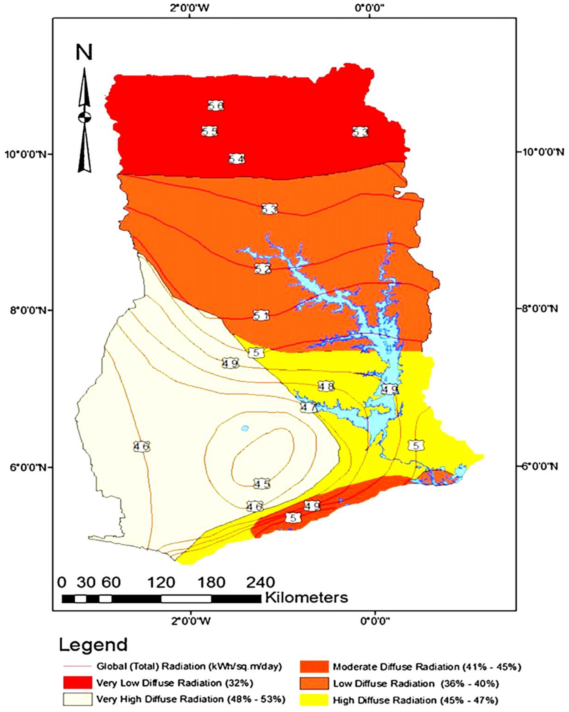
1.3.1. Electrification Challenges in Ghana
1.3.2. Solar-Powered Microgrids as a Solution
1.3.3. Technical Considerations for Micro Grid Implementation
1.3.4. Power Flow Methods
1.3.5. Economic Indices of Solar PV Projects
2. Methodology
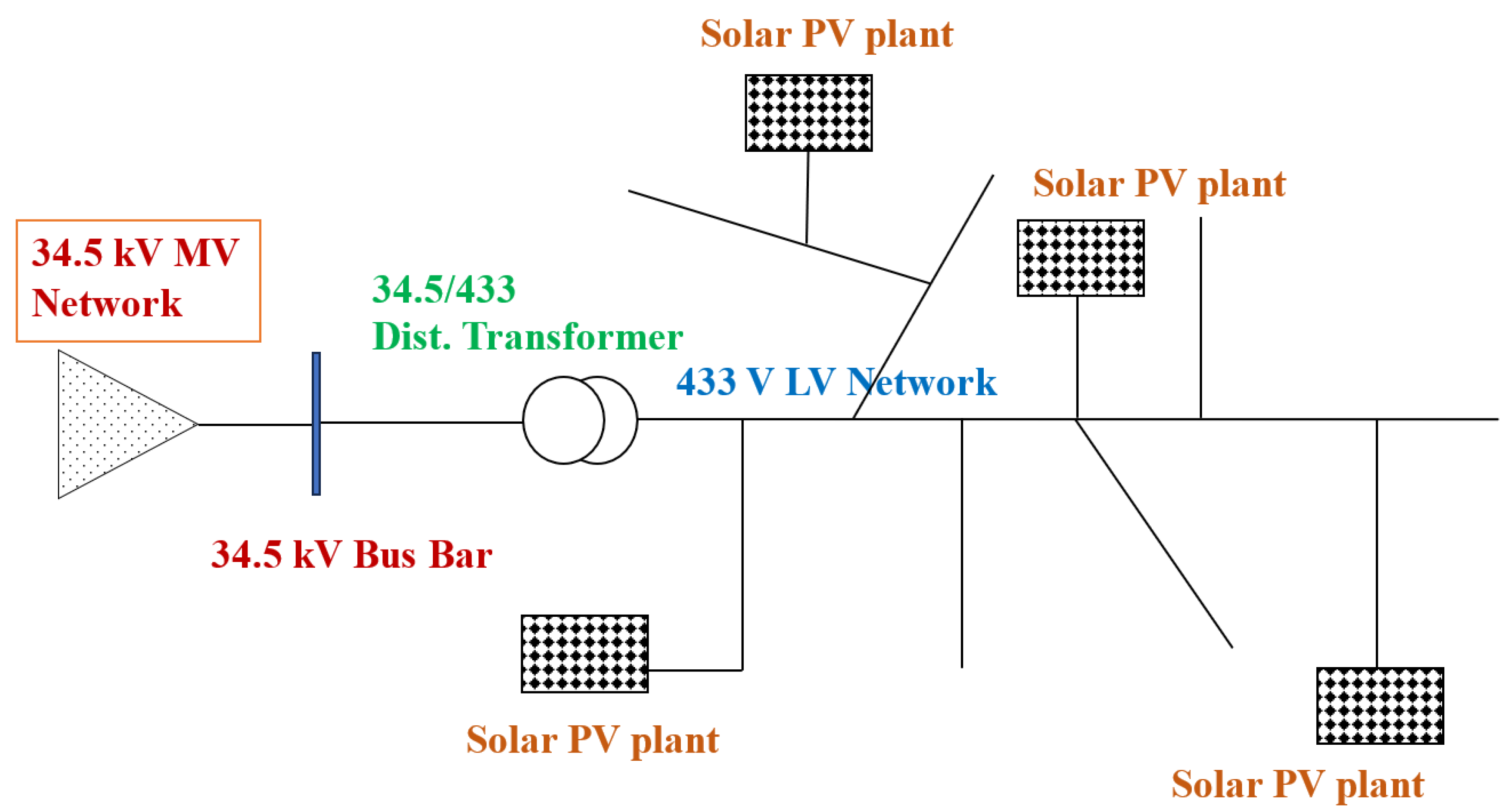
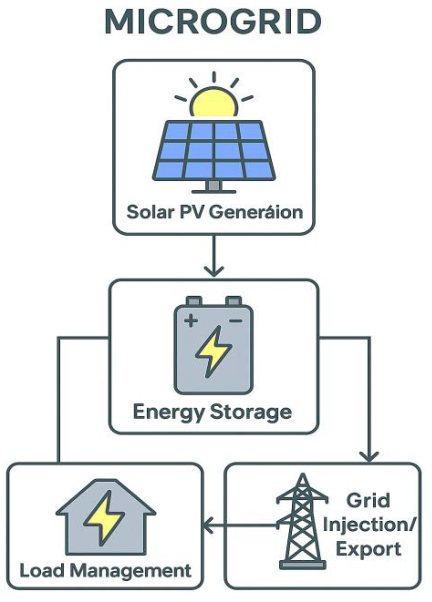
2.1. LV Microgrid Concept and Definition
2.2. Load Model and Management Strategy
2.3. Grid Impact
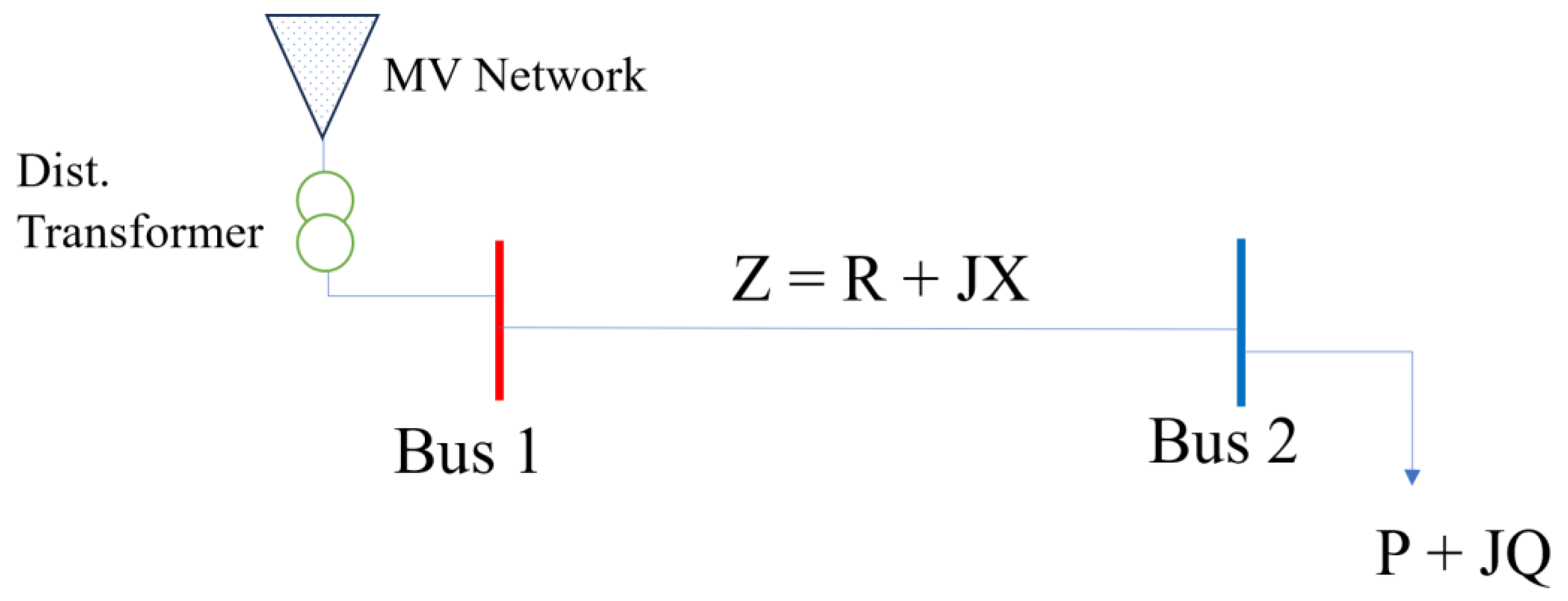
2.4. Load Flow
- 1.
- Input parameters: the inputs parameters include number of nodes or buses; load (P + Q) buses: bus voltage limits (Vmin, Vmax): line impedances (R + jX); line section length (Li); line capacity (amps); PV size (kWp); and RPS size (kVAr);
- 2.
- Base case: Firstly, compute In using the BIBC [a] and Iload, expressed in Equation (12). Calculate the bus voltages using the BCBV [b] matrices in Equation (13). The impedance matrix is formed by multiplying the BCBV matrix and the line impedance matrix (Z). In this context, In represents the current in the n-th branch, Ii is the n-th load current, and Inpv is the injection of the n-th PV system into the network;
- 3.
- Calculate the following power flows as follows:
- 4.
- Apparent (Ssec), active, and reactive powers in the lines using Equation (14);
- 5.
- Lines losses (Lossline) active and reactive losses are determined using Equation (15);
- 6.
- Apparent (Sinjected), active, and reactive powers injections by using (16);
- 7.
- Iterate the process to determine the penetration for various PV injections;
- 8.
- Check whether the reactive power requirement is met with the PV injections. If yes, end the process; if no, execute step 4;
- 9.
- Repeat the process from 2 to include reactive power compensation (RSP)
2.5. Supercapacitor Model
2.6. Case Study Analysis
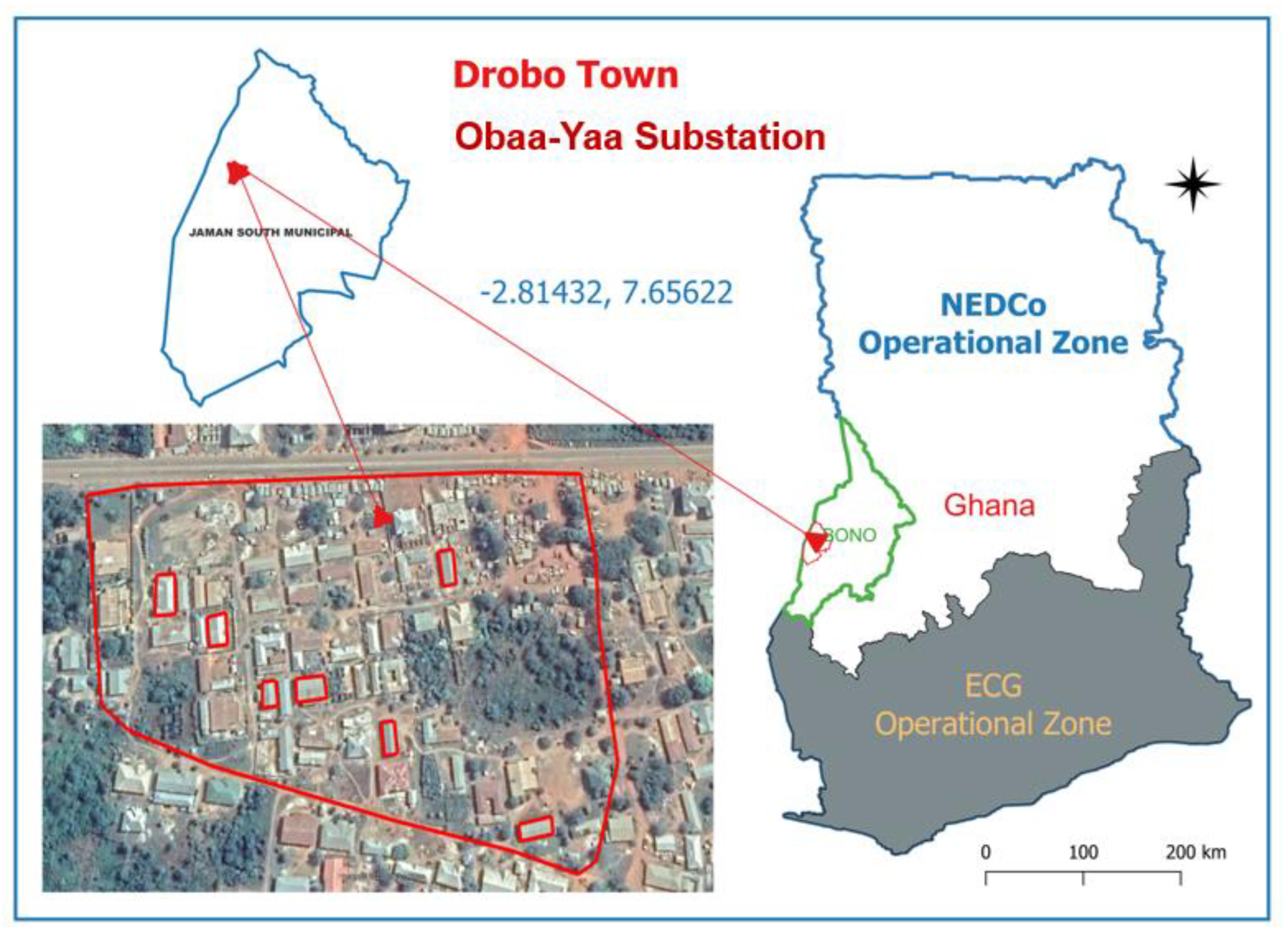
2.6.1. Solar PV Electricity for Grid-to-Microgrid Conversion
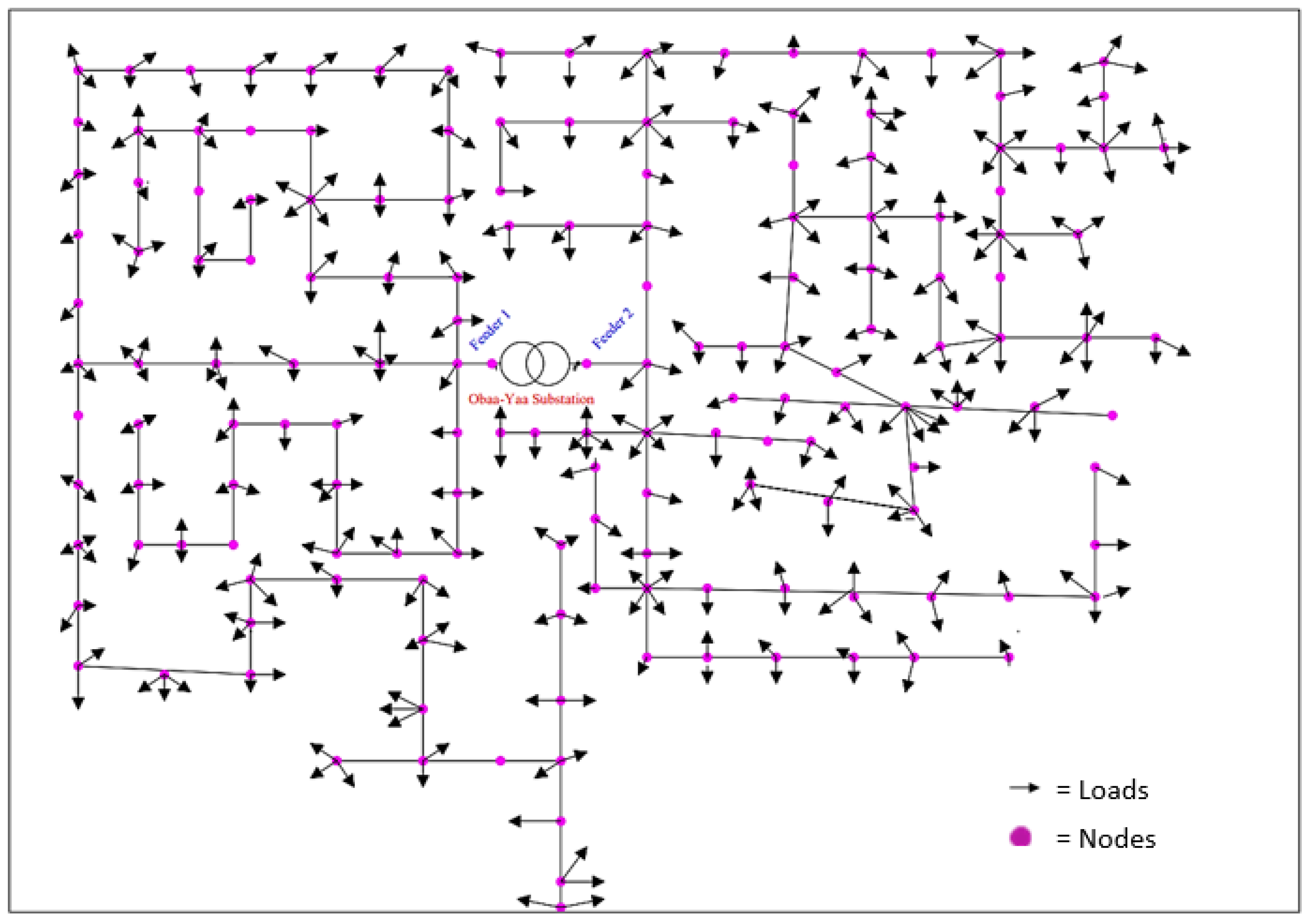
2.6.2. Data Collection—Network and Consumer Data
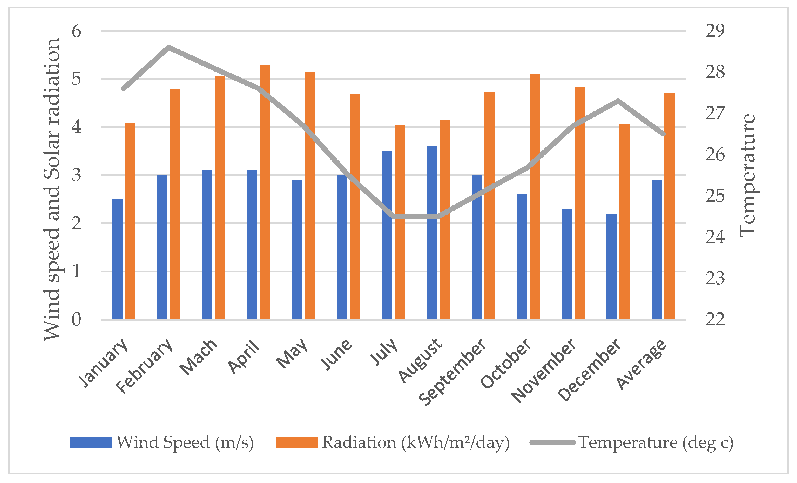
2.6.3. Solar PV System Sizing
2.7. Python Simulation
- 1.
- Base case: simulating the actual state of the LV network with PV and RSP injections;
- 2.
- Scenario 1: simulation with the base case information and PV injections;
- 3.
- Scenario 2: simulation with the base case information, PV, and RSP (natural) injection;
- 4.
- Scenario 3: simulation with base case information, PV, and RSP (optimised) injection.
2.8. Economic Analysis
2.8.1. Cost Analysis
2.8.2. Revenue Generation
2.9. Economic Evaluation
3. Results and Discussion
3.1. Load Flow Results
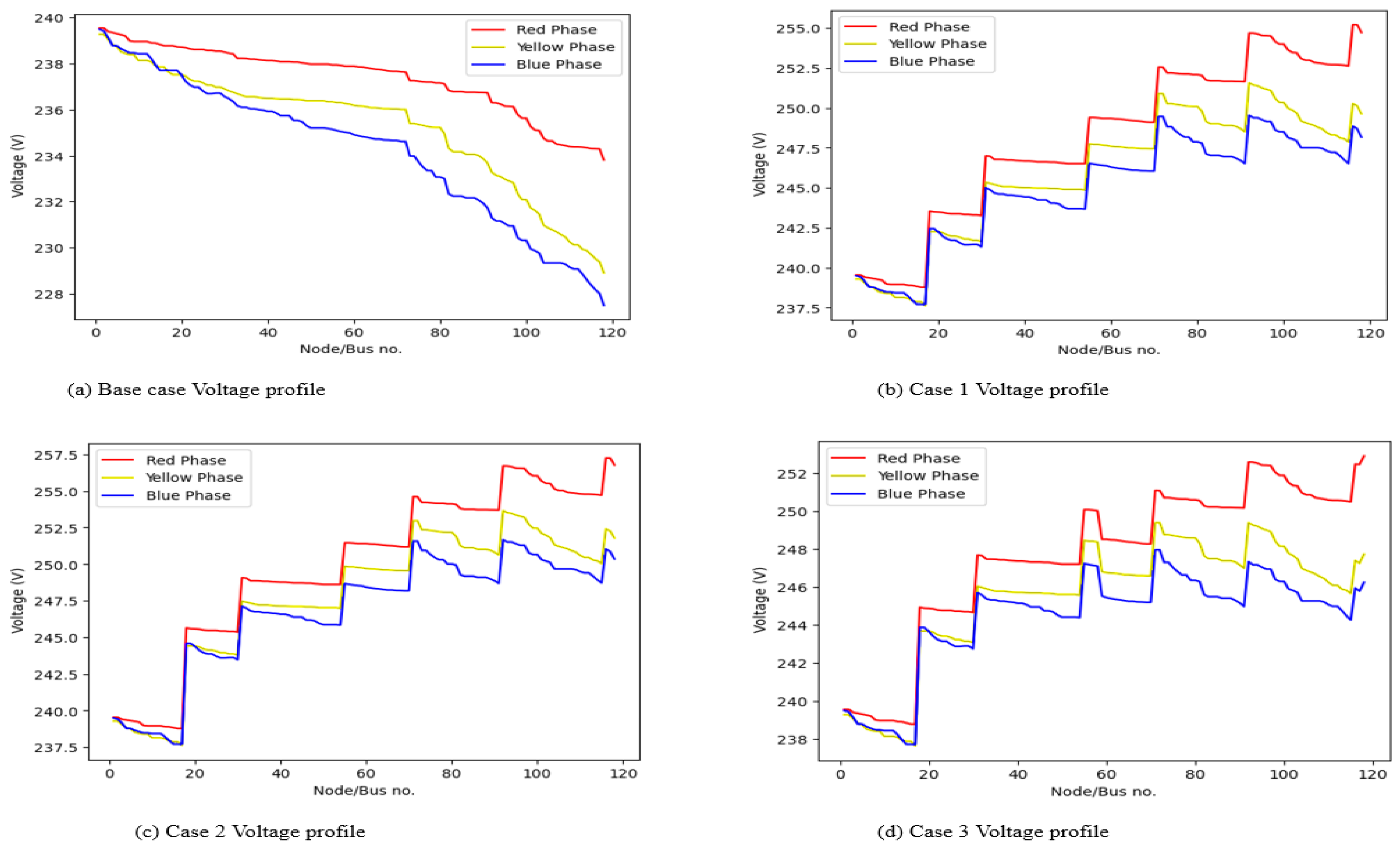
3.1.1. Voltage Profile
3.1.2. Power Flows
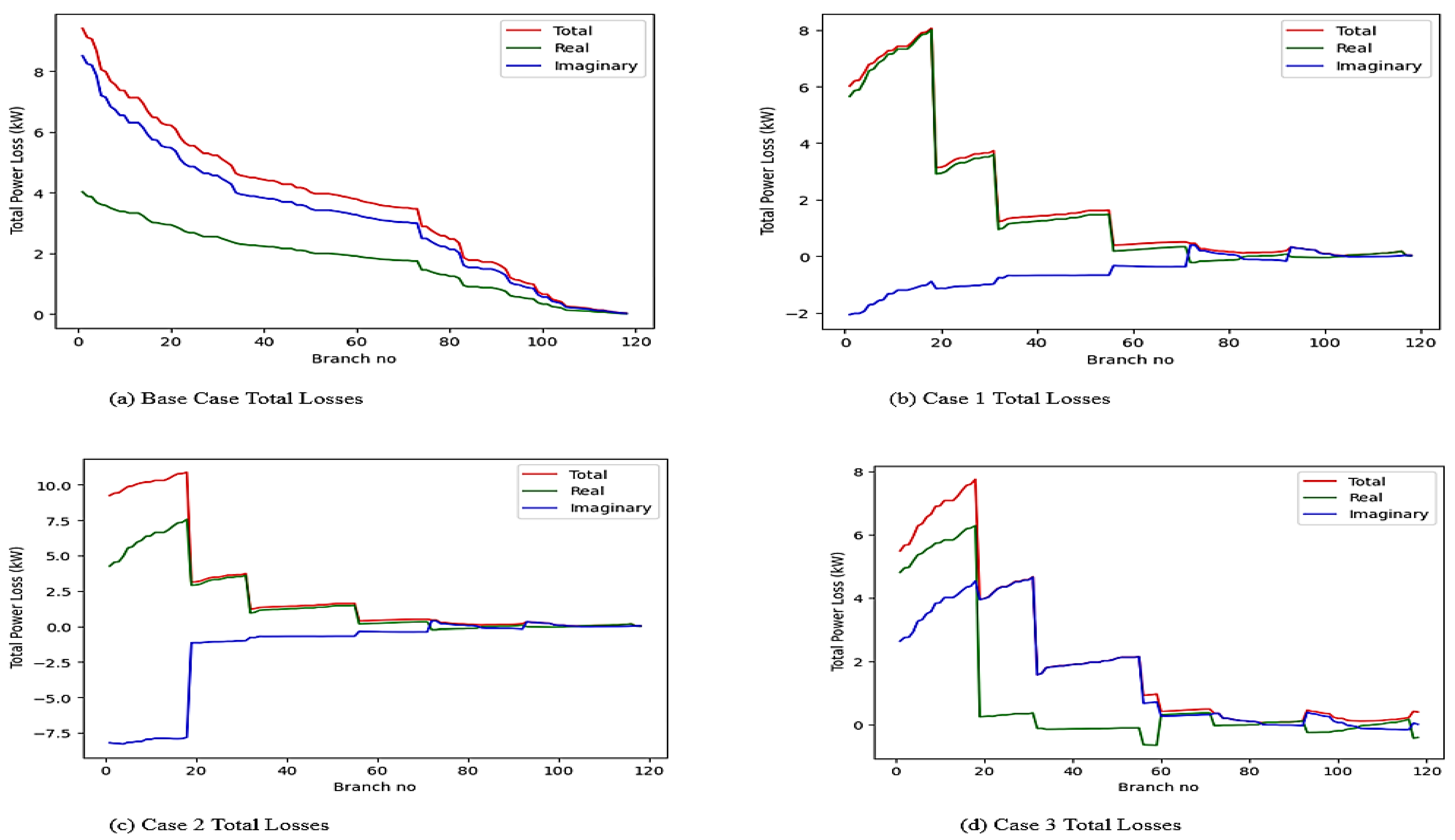
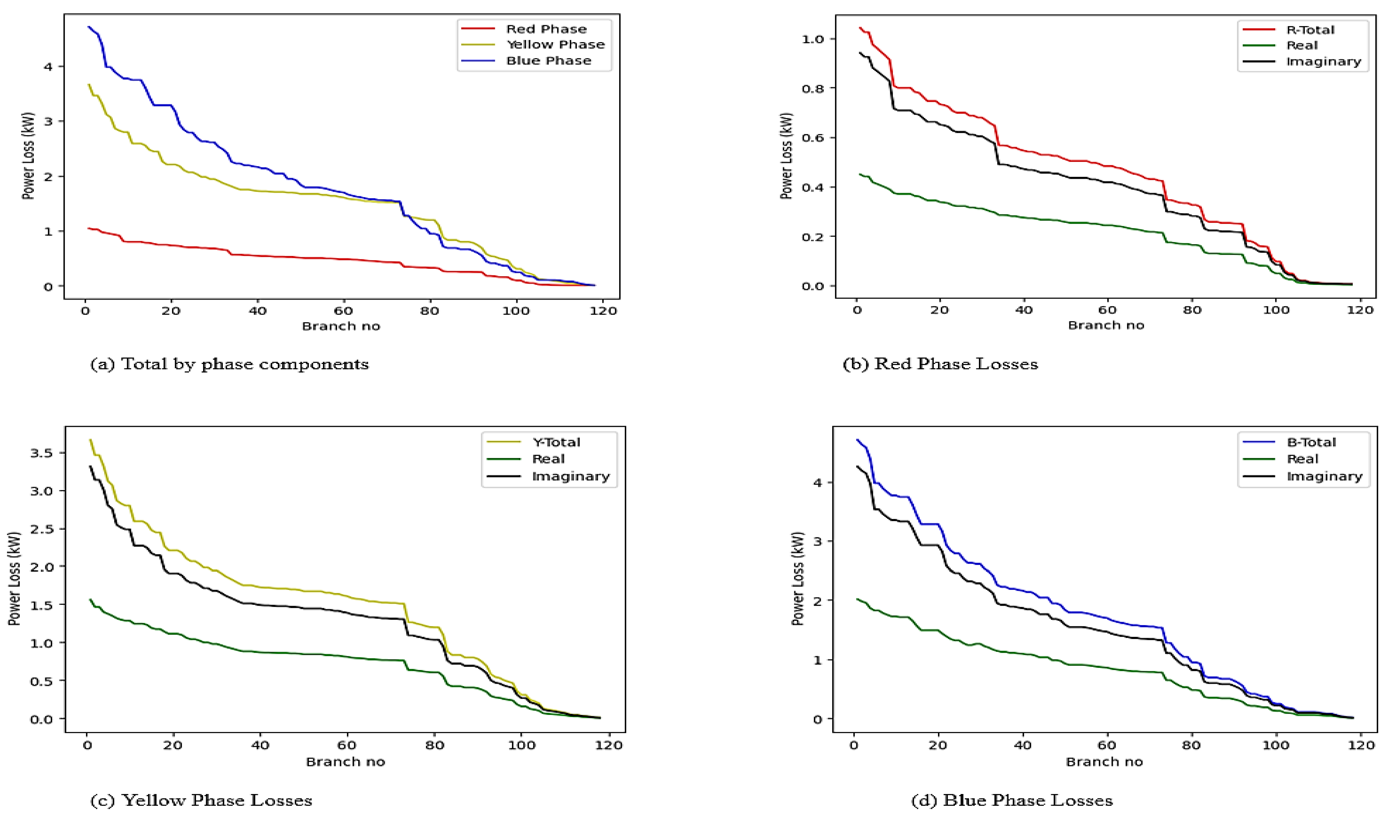
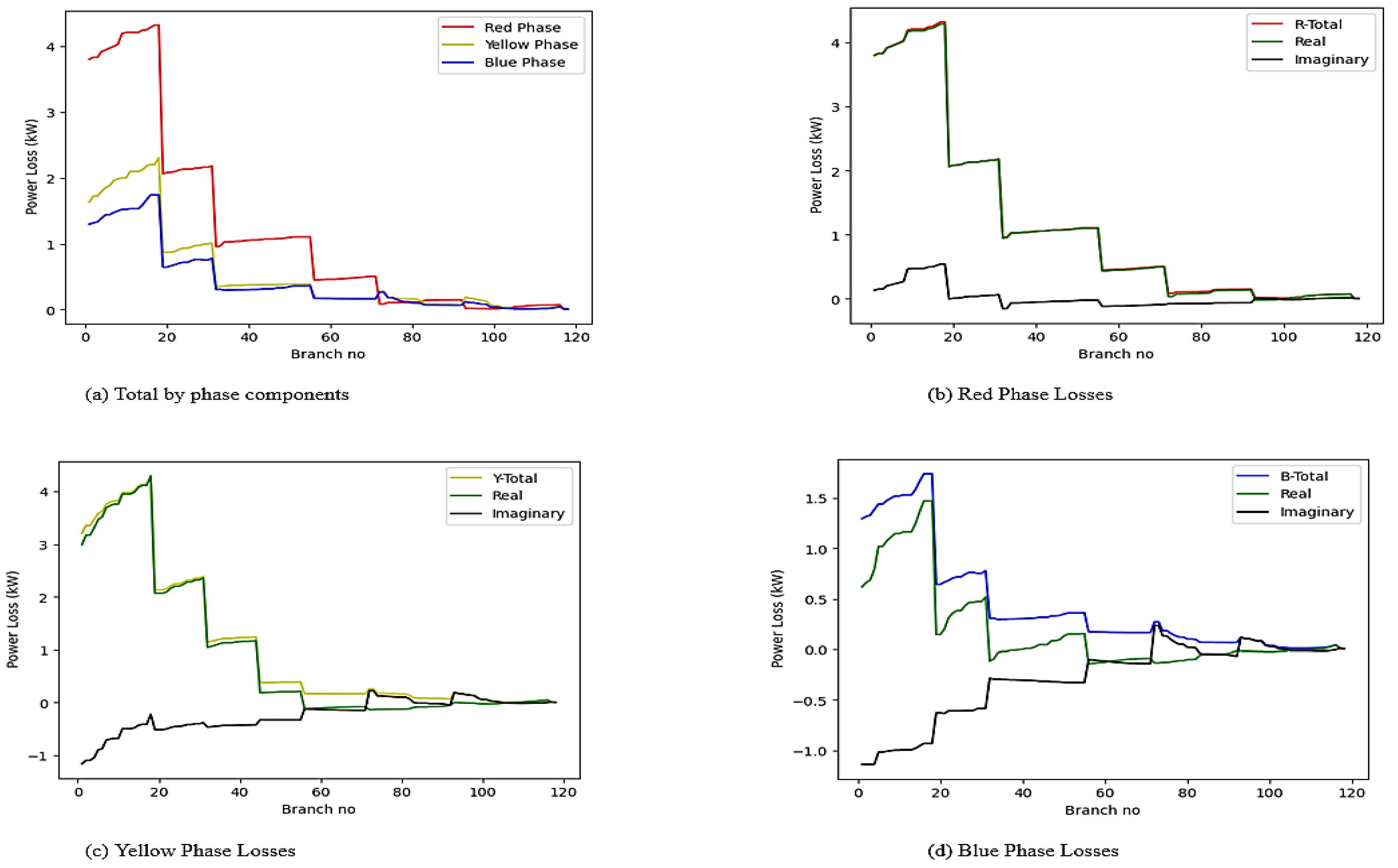
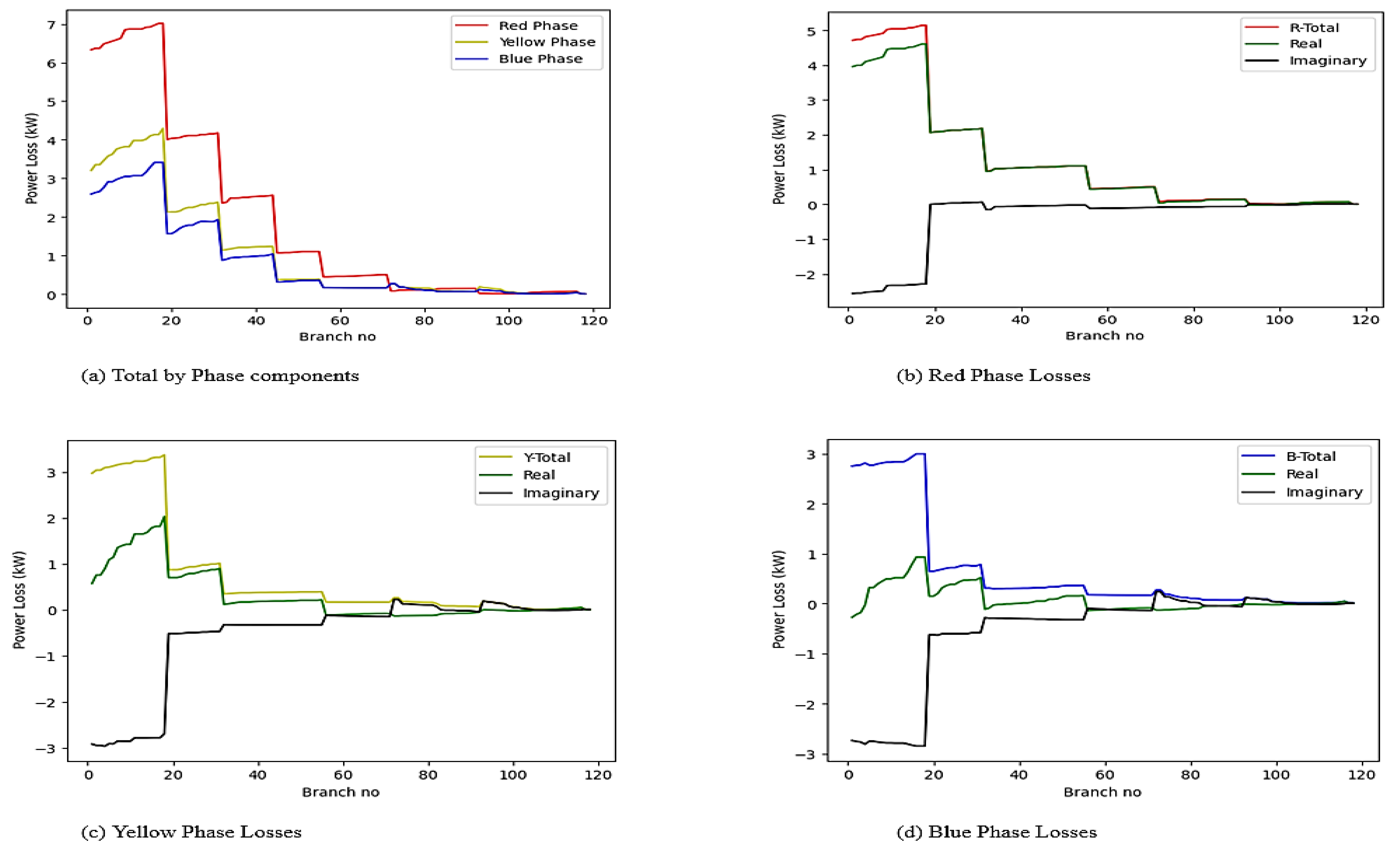
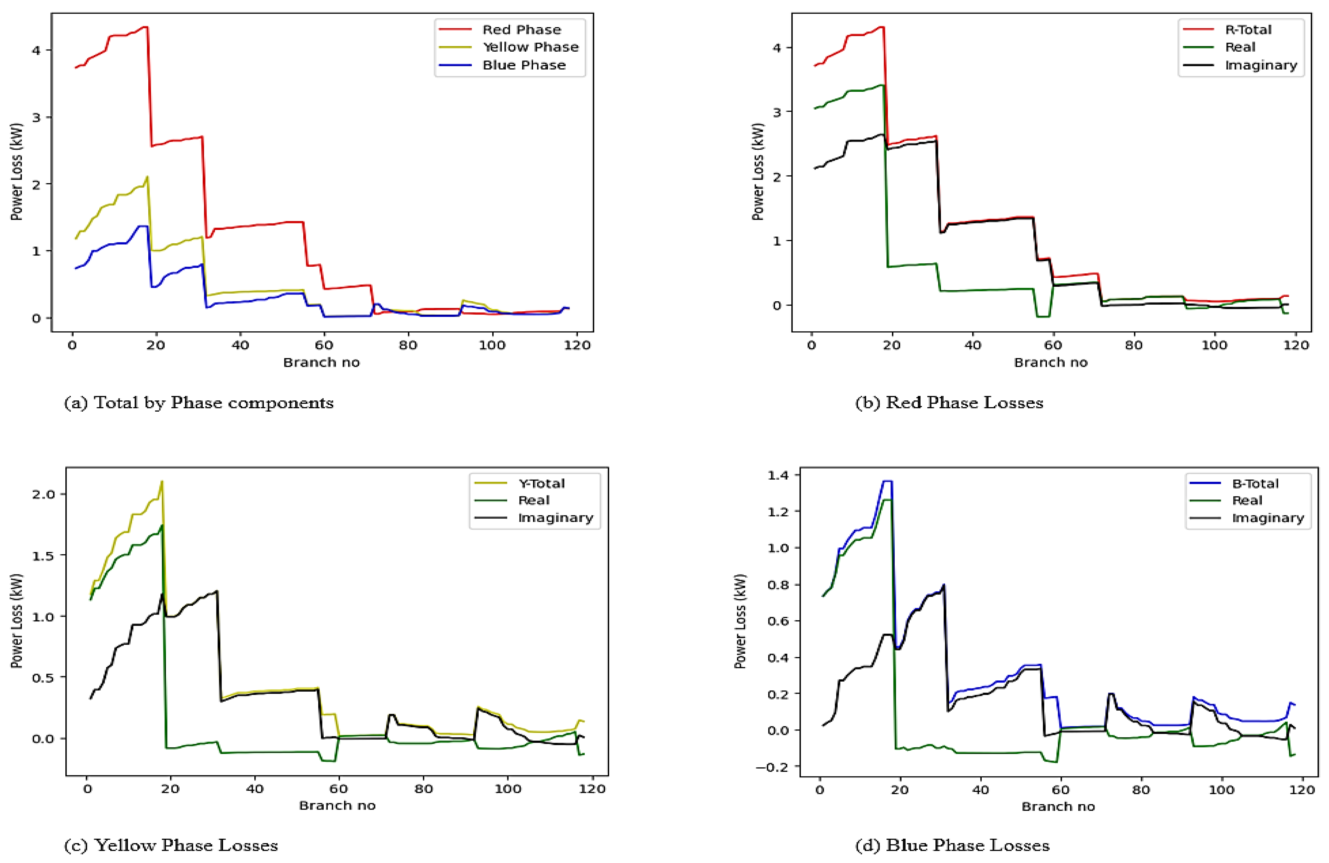
3.1.3. Losses
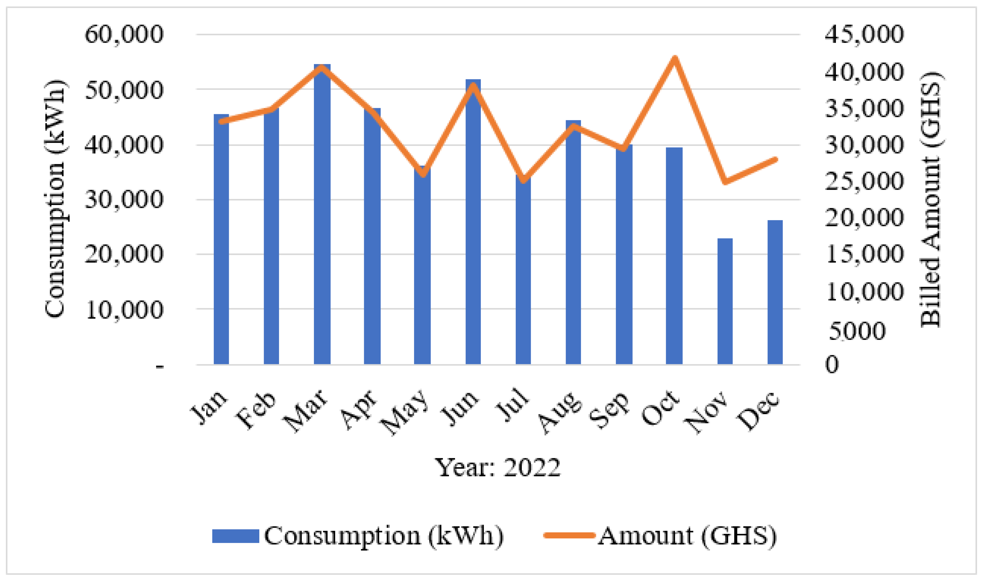
3.2. Consumer Demand Analysis
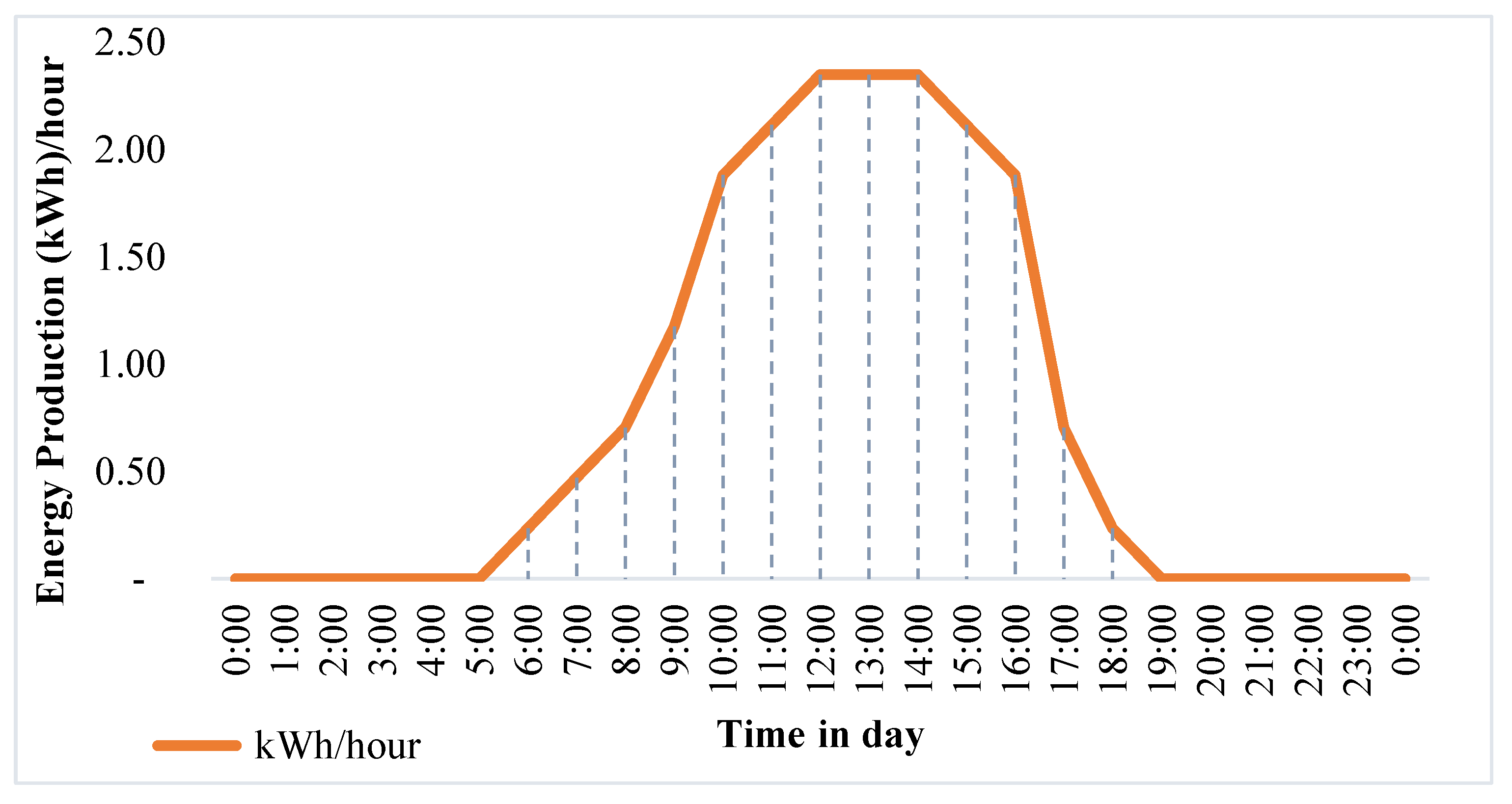
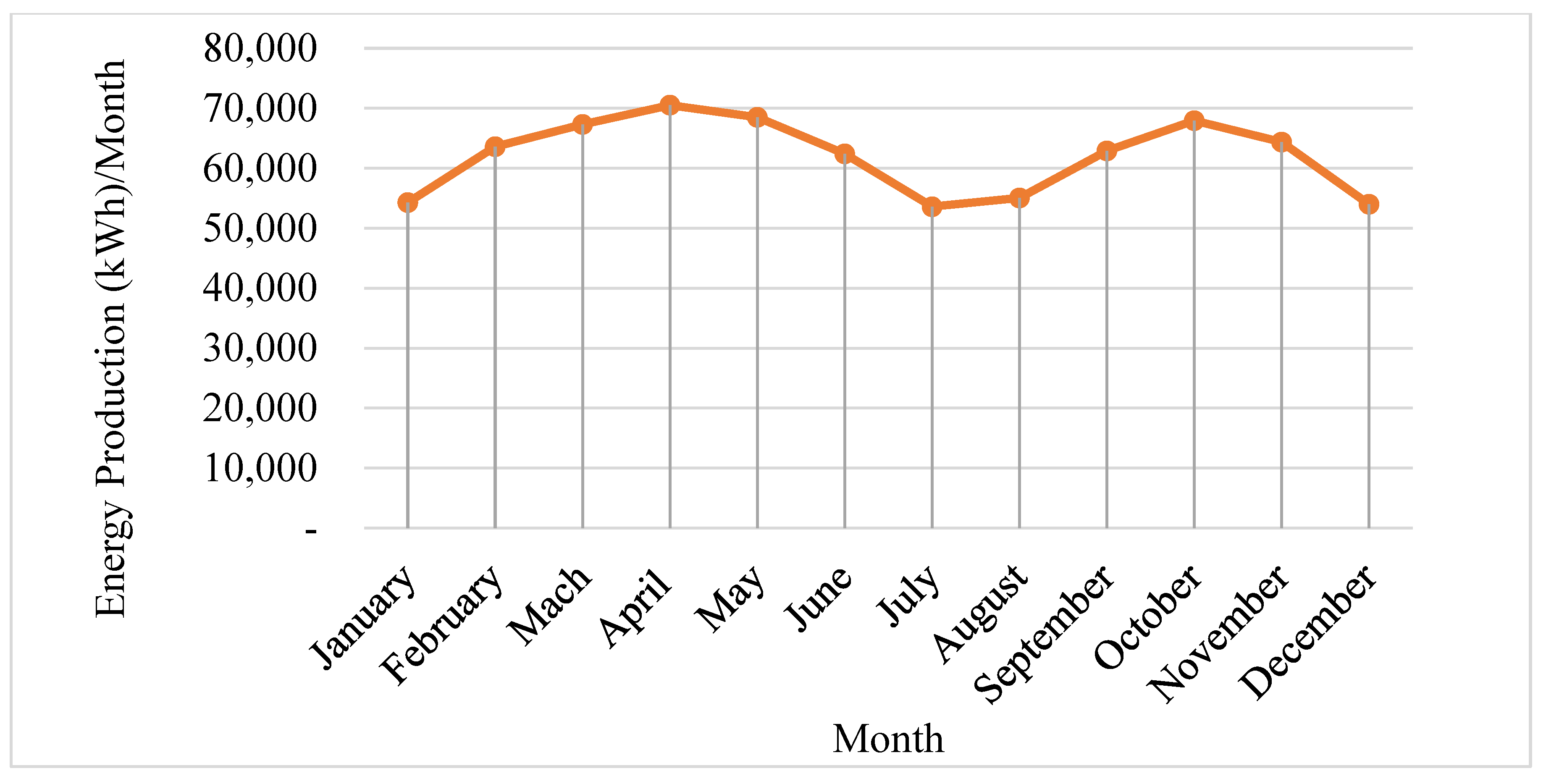
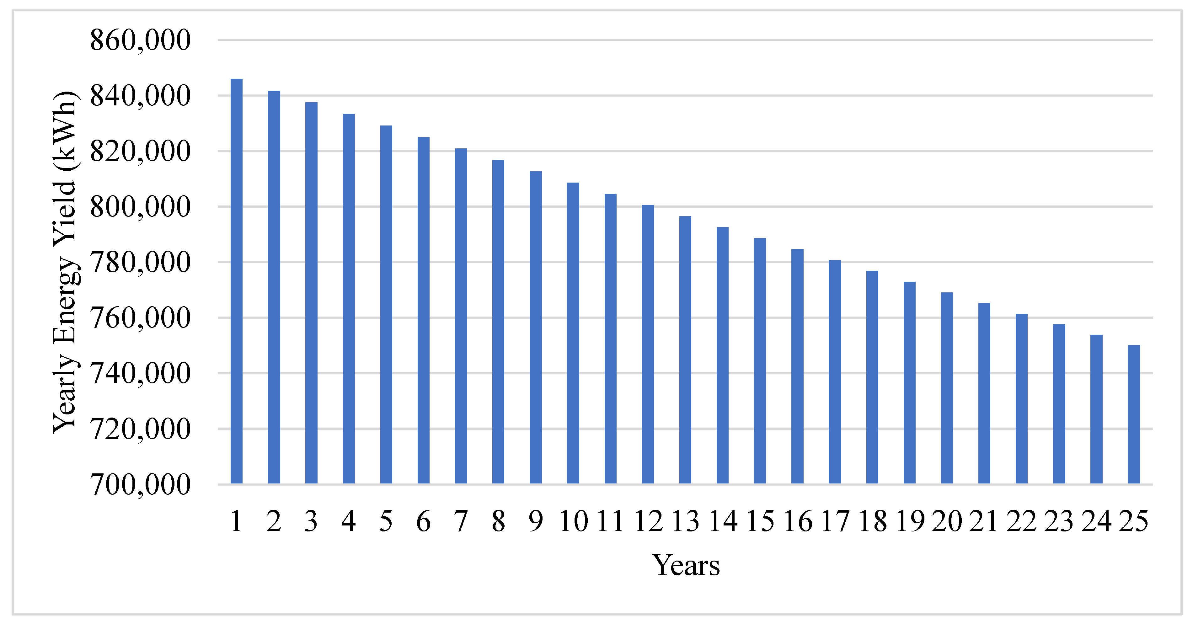
3.3. PV Energy Production and Economics
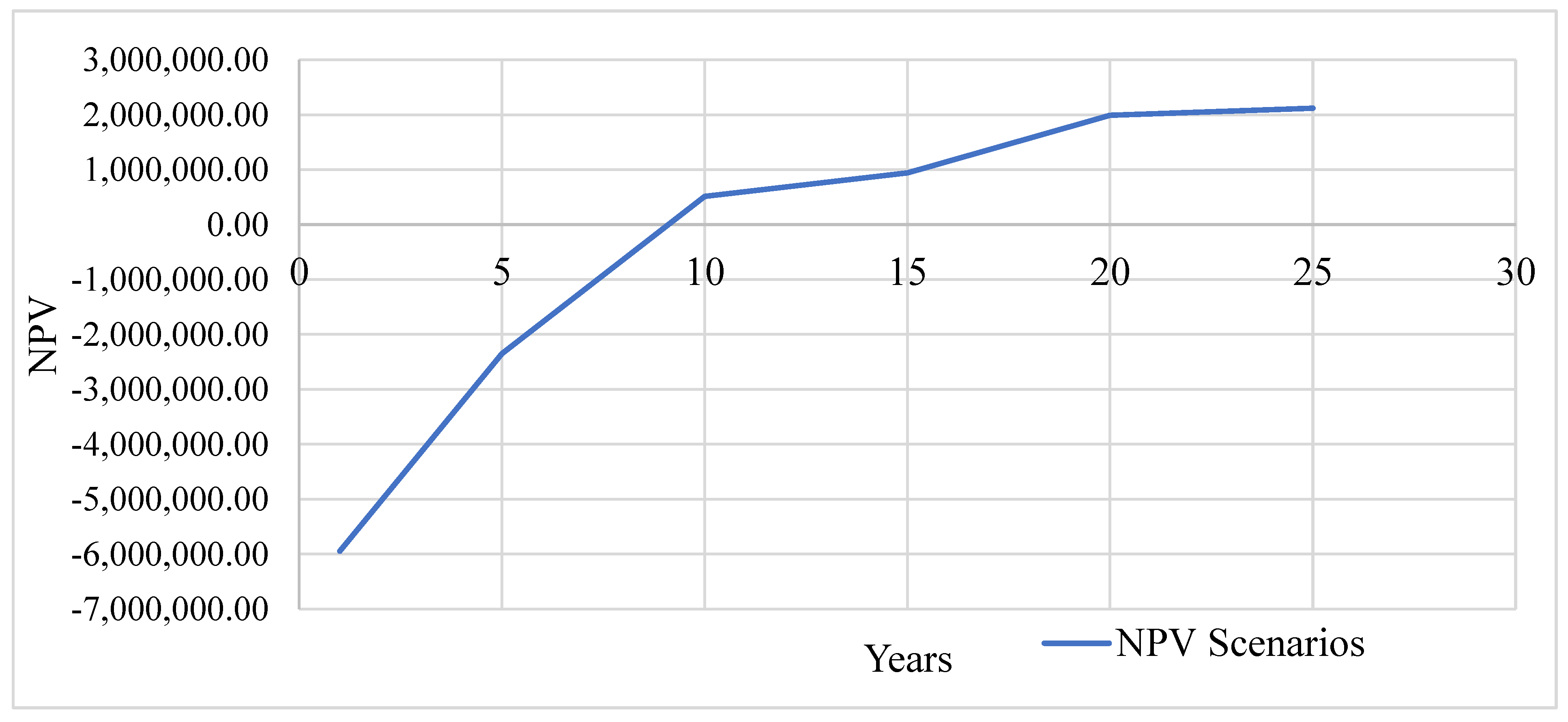
3.4. The Conventional LV Grid-to-Microgrid Conversion Economics
3.5. Policy Implications
3.6. Future Research and Recommendations
4. Conclusions
- a.
- The cost of replacing the existing LV grid infrastructure was not considered in this work and it could potentially reduce the financial prospect;
- b.
- Ghana’s rainy season (June–September) reduces PV output, which introduces very high intermittencies during the period, necessitating grid backup or hybrid systems.
Author Contributions
Funding
Data Availability Statement
Conflicts of Interest
Appendix A. Load, PV Generation, and RSP Capacities
| Node No. | Load kVA | Measured Load Terminal Voltage (V) | PV (kWp) | RPS (kVAr) | |||||
| R | Y | B | R-N | Y-N | B-N | Natural | Optimised | ||
| 1 | 0.27 | 1.61 | 0.55 | 241.9 | 243.6 | 239.6 | |||
| 2 | 0.00 | 0.00 | 0.36 | 241.7 | 243.5 | 239.4 | |||
| 3 | 0.77 | 1.19 | 1.39 | 241.6 | 243.2 | 239.2 | |||
| 4 | 0.21 | 0.36 | 0.45 | 241.4 | 242.9 | 239.1 | |||
| 5 | 0.24 | 0.46 | 0.00 | 241.2 | 242.6 | 238.9 | |||
| 6 | 0.24 | 0.48 | 0.68 | 241.1 | 242.3 | 238.7 | 2.3 | ||
| 7 | 0.26 | 0.36 | 0.47 | 240.9 | 242.0 | 238.5 | |||
| 8 | 0.43 | 0.24 | 0.43 | 240.7 | 241.7 | 238.3 | |||
| 9 | 0.14 | 0.00 | 0.00 | 240.6 | 241.4 | 238.2 | |||
| 10 | 0.00 | 0.63 | 0.21 | 240.4 | 241.1 | 238.0 | 93 | 2.3 | |
| 11 | 0.00 | 0.00 | 0.00 | 240.2 | 240.8 | 237.8 | |||
| 12 | 0.00 | 0.00 | 0.00 | 240.0 | 240.5 | 237.6 | |||
| 13 | 0.29 | 0.31 | 1.04 | 239.9 | 240.2 | 237.4 | |||
| 14 | 0.05 | 0.79 | 1.42 | 239.7 | 239.9 | 237.3 | |||
| 15 | 0.29 | 0.29 | 1.23 | 239.5 | 239.6 | 237.1 | |||
| 16 | 0.29 | 0.00 | 0.00 | 239.4 | 239.3 | 236.9 | |||
| 17 | 0.00 | 0.53 | 0.00 | 239.2 | 239.0 | 236.7 | 2.9 | ||
| 18 | 0.00 | 0.55 | 0.00 | 239.0 | 238.7 | 236.5 | 73 | 2.9 | |
| 19 | 0.24 | 0.00 | 0.00 | 238.9 | 238.4 | 236.4 | |||
| 20 | 0.05 | 0.00 | 1.02 | 238.7 | 238.1 | 236.2 | |||
| 21 | 0.12 | 0.31 | 0.76 | 238.5 | 237.8 | 236.0 | |||
| 22 | 0.31 | 0.76 | 0.83 | 238.3 | 237.5 | 235.8 | |||
| 23 | 0.13 | 0.39 | 0.45 | 238.2 | 237.2 | 235.6 | |||
| 24 | 0.00 | 0.00 | 0.00 | 238.0 | 236.9 | 235.5 | |||
| 25 | 0.00 | 0.36 | 0.87 | 237.8 | 236.6 | 235.3 | |||
| 26 | 0.21 | 0.52 | 0.59 | 237.7 | 236.3 | 235.1 | |||
| 27 | 0.00 | 0.00 | 0.00 | 237.5 | 236.0 | 234.9 | |||
| 28 | 0.14 | 0.42 | 1.12 | 237.3 | 235.7 | 234.7 | |||
| 29 | 0.00 | 0.00 | 0.00 | 237.2 | 235.4 | 234.6 | |||
| 30 | 0.21 | 0.36 | 0.78 | 237.0 | 235.1 | 234.4 | |||
| 31 | 0.23 | 0.44 | 0.42 | 236.8 | 234.8 | 234.2 | 59 | 3.7 | 3.7 |
| 32 | 0.15 | 0.33 | 0.67 | 236.6 | 234.5 | 234.0 | |||
| 33 | 0.28 | 0.33 | 0.29 | 236.5 | 234.2 | 233.8 | |||
| 34 | 0.00 | 0.36 | 0.31 | 236.3 | 233.9 | 233.7 | |||
| 35 | 0.03 | 0.31 | 0.00 | 236.1 | 233.6 | 233.5 | |||
| 36 | 0.15 | 0.00 | 0.34 | 236.0 | 233.3 | 233.3 | |||
| 37 | 0.00 | 0.00 | 0.00 | 235.8 | 233.0 | 233.1 | |||
| 38 | 0.15 | 0.17 | 0.20 | 235.6 | 232.7 | 232.9 | |||
| 39 | 0.08 | 0.13 | 0.10 | 235.5 | 232.4 | 232.8 | |||
| 40 | 0.08 | 0.05 | 0.26 | 235.3 | 232.1 | 232.6 | |||
| 41 | 0.00 | 0.00 | 0.00 | 235.1 | 231.8 | 232.4 | |||
| 42 | 0.10 | 0.08 | 0.38 | 234.9 | 231.5 | 232.2 | |||
| 43 | 0.15 | 0.06 | 0.61 | 234.8 | 231.2 | 232.0 | |||
| 44 | 0.00 | 0.00 | 0.00 | 234.6 | 230.9 | 231.9 | 65 | 4.8 | 4.8 |
| 45 | 0.00 | 0.00 | 0.00 | 234.4 | 230.6 | 231.7 | |||
| 46 | 0.08 | 0.13 | 1.03 | 234.3 | 230.3 | 231.5 | |||
| 47 | 0.00 | 0.00 | 0.00 | 234.1 | 230.0 | 231.3 | |||
| 48 | 0.18 | 0.08 | 0.30 | 233.9 | 229.7 | 231.1 | |||
| 49 | 0.13 | 0.19 | 0.91 | 233.8 | 229.4 | 231.0 | |||
| 50 | 0.14 | 0.00 | 0.51 | 233.6 | 229.1 | 230.8 | |||
| 51 | 0.00 | 0.00 | 0.00 | 233.4 | 228.8 | 230.6 | |||
| 52 | 0.00 | 0.00 | 0.00 | 233.2 | 228.5 | 230.4 | |||
| 53 | 0.00 | 0.00 | 0.00 | 233.1 | 228.2 | 230.2 | |||
| 54 | 0.00 | 0.22 | 0.13 | 232.9 | 227.9 | 230.1 | |||
| 55 | 0.15 | 0.00 | 0.17 | 232.7 | 227.6 | 229.9 | 45 | 4 | 4 |
| 56 | 0.00 | 0.19 | 0.25 | 232.6 | 227.3 | 229.7 | |||
| 57 | 0.12 | 0.00 | 0.22 | 232.4 | 227.0 | 229.5 | |||
| 58 | 0.16 | 0.23 | 0.18 | 232.2 | 226.7 | 229.3 | |||
| 59 | 0.00 | 0.13 | 0.12 | 232.1 | 226.4 | 229.2 | |||
| 60 | 0.00 | 0.28 | 0.44 | 231.9 | 226.1 | 229.0 | |||
| 61 | 0.15 | 0.13 | 0.24 | 231.7 | 225.8 | 228.8 | |||
| 62 | 0.05 | 0.05 | 0.22 | 231.5 | 225.5 | 228.6 | |||
| 63 | 0.15 | 0.15 | 0.13 | 231.4 | 225.2 | 228.4 | |||
| 64 | 0.18 | 0.20 | 0.22 | 231.2 | 224.9 | 228.3 | |||
| 65 | 0.15 | 0.00 | 0.19 | 231.0 | 224.6 | 228.1 | |||
| 66 | 0.07 | 0.10 | 0.00 | 230.9 | 224.3 | 227.9 | |||
| 67 | 0.15 | 0.10 | 0.17 | 230.7 | 224.0 | 227.7 | |||
| 68 | 0.21 | 0.00 | 0.03 | 230.5 | 223.7 | 227.5 | |||
| 69 | 0.08 | 0.05 | 0.07 | 230.4 | 223.4 | 227.4 | |||
| 70 | 0.00 | 0.00 | 0.00 | 230.2 | 223.1 | 227.2 | 54 | 4 | 4 |
| 71 | 0.13 | 0.10 | 0.22 | 230.0 | 222.8 | 227.0 | |||
| 72 | 0.05 | 0.00 | 0.00 | 229.8 | 222.5 | 226.8 | |||
| 73 | 1.88 | 3.16 | 3.28 | 229.7 | 222.2 | 226.6 | |||
| 74 | 0.00 | 0.00 | 0.00 | 229.5 | 221.9 | 226.5 | |||
| 75 | 0.14 | 0.24 | 1.34 | 229.3 | 221.6 | 226.3 | |||
| 76 | 0.14 | 0.18 | 1.11 | 229.2 | 221.3 | 226.1 | |||
| 77 | 0.05 | 0.25 | 0.86 | 229.0 | 221.0 | 225.9 | |||
| 78 | 0.00 | 0.18 | 0.00 | 228.8 | 220.7 | 225.7 | |||
| 79 | 0.20 | 0.05 | 1.43 | 228.7 | 220.4 | 225.6 | |||
| 80 | 0.00 | 0.00 | 0.00 | 228.5 | 220.1 | 225.4 | |||
| 81 | 0.21 | 1.36 | 0.35 | 228.3 | 219.8 | 225.2 | |||
| 82 | 1.44 | 3.34 | 3.49 | 228.1 | 219.5 | 225.0 | |||
| 83 | 0.25 | 0.75 | 0.49 | 228.0 | 219.2 | 224.8 | |||
| 84 | 0.00 | 0.00 | 0.00 | 227.8 | 218.9 | 224.7 | |||
| 85 | 0.00 | 0.00 | 0.00 | 227.6 | 218.6 | 224.5 | |||
| 86 | 0.14 | 0.57 | 0.40 | 227.5 | 218.3 | 224.3 | |||
| 87 | 0.00 | 0.00 | 0.00 | 227.3 | 218.0 | 224.1 | |||
| 88 | 0.00 | 0.00 | 0.00 | 227.1 | 217.7 | 223.9 | |||
| 89 | 0.05 | 0.31 | 0.58 | 227.0 | 217.4 | 223.8 | |||
| 90 | 0.02 | 0.69 | 0.70 | 226.8 | 217.1 | 223.6 | |||
| 91 | 0.05 | 0.95 | 0.96 | 226.6 | 216.8 | 223.4 | |||
| 92 | 2.22 | 2.10 | 2.28 | 226.4 | 216.5 | 223.2 | 4 | 4 | |
| 93 | 0.05 | 0.69 | 0.76 | 226.3 | 216.2 | 223.0 | |||
| 94 | 0.25 | 0.26 | 0.00 | 226.1 | 215.9 | 222.9 | |||
| 95 | 0.47 | 0.63 | 0.62 | 225.9 | 215.6 | 222.7 | |||
| 96 | 0.05 | 0.41 | 0.53 | 225.8 | 215.3 | 222.5 | |||
| 97 | 0.07 | 0.39 | 0.00 | 225.6 | 215.0 | 222.3 | |||
| 98 | 1.80 | 2.49 | 2.71 | 225.4 | 214.7 | 222.1 | |||
| 99 | 0.74 | 1.33 | 0.55 | 225.3 | 214.4 | 222.0 | |||
| 100 | 0.00 | 0.00 | 0.00 | 225.1 | 214.1 | 221.8 | |||
| 101 | 1.91 | 1.84 | 1.97 | 224.9 | 213.8 | 221.6 | |||
| 102 | 0.74 | 0.60 | 0.41 | 224.7 | 213.5 | 221.4 | |||
| 103 | 0.10 | 0.87 | 0.53 | 224.6 | 213.2 | 221.2 | |||
| 104 | 1.80 | 2.52 | 2.26 | 224.4 | 212.9 | 221.1 | |||
| 105 | 0.54 | 0.55 | 0.00 | 224.2 | 212.6 | 220.9 | |||
| 106 | 0.00 | 0.45 | 0.00 | 224.1 | 212.3 | 220.7 | |||
| 107 | 0.69 | 0.47 | 0.00 | 223.9 | 212.0 | 220.5 | |||
| 108 | 0.18 | 0.66 | 0.00 | 223.7 | 211.7 | 220.3 | |||
| 109 | 0.18 | 0.51 | 0.26 | 223.6 | 211.4 | 220.2 | |||
| 110 | 0.25 | 1.14 | 0.75 | 223.4 | 211.1 | 220.0 | |||
| 111 | 0.09 | 0.72 | 0.40 | 223.2 | 210.8 | 219.8 | |||
| 112 | 0.00 | 0.00 | 0.00 | 223.0 | 210.5 | 219.6 | |||
| 113 | 0.07 | 1.01 | 1.12 | 222.9 | 210.2 | 219.4 | |||
| 114 | 0.11 | 0.25 | 1.36 | 222.7 | 209.9 | 219.3 | |||
| 115 | 0.20 | 0.92 | 1.14 | 222.5 | 209.6 | 219.1 | |||
| 116 | 0.04 | 0.96 | 1.18 | 222.4 | 209.3 | 218.9 | 40 | 5.4 | 5.4 |
| 117 | 0.04 | 0.71 | 0.83 | 222.2 | 209.0 | 218.7 | |||
| 118 | 2.46 | 2.55 | 2.73 | 222.0 | 208.7 | 218.5 | |||
| Total | 28.29 | 52.58 | 61.38 | 429.19 | 31.10 | 31.10 | |||
References
- Peprah, F.; Gyamfi, S.; Amo-boateng, M.; Effah-donyina, E. Impact assessment of grid tied rooftop PV systems on LV distribution network. Sci. Afr. 2022, 16, e01172. [Google Scholar] [CrossRef]
- Asante, K.; Gyamfi, S.; Amo-Boateng, M. Techno-economic analysis of waste-to-energy with solar hybrid: A case study from Kumasi, Ghana. Sol. Compass 2023, 6, 100041. [Google Scholar] [CrossRef]
- Peprah, F.; Gyamfi, S.; Effah-donyina, E.; Amo-boateng, M. e-Prime-Advances in Electrical Engineering, Electronics and Energy Evaluation of reactive power support in solar PV prosumer grid. e-Prime-Adv. Electr. Eng. Electron. Energy 2022, 2, 100057. [Google Scholar] [CrossRef]
- Poongothai, S.; Srinath, S. Power quality enhancement in solar power with grid connected system using UPQC. Microprocess Microsyst. 2020, 79, 103300. [Google Scholar] [CrossRef]
- Sechilariu, M.; Locment, F. Urban DC Microgrid: Intelligent Control and Power Flow Optimization, 1st ed.; Elsevier: Amsterdam, The Netherland, 2016. [Google Scholar]
- Tavakoli, A.; Saha, S.; Arif, M.T.; Haque, M.E.; Mendis, N.; Oo, A.M.T. Impacts of grid integration of solar PV and electric vehicle on grid stability, power quality and energy economics: A review. IET Energy Syst Integr. 2020, 2, 215–225. [Google Scholar] [CrossRef]
- Kaushal, J.; Basak, P. Power quality control based on voltage sag/swell, unbalancing, frequency, THD and power factor using artificial neural network in PV integrated AC microgrid. Sustain. Energy Grids Netw. 2020, 23, 100365. [Google Scholar] [CrossRef]
- Radwan, A.A.; Zaki Diab, A.A.; Elsayed, A.H.M.; Alhelou, H.H.; Siano, P. Active distribution network modeling for enhancing sustainable power system performance; a case study in Egypt. Sustainability 2020, 12, 8991. [Google Scholar] [CrossRef]
- Zapata Riveros, J.; Kubli, M.; Ulli-Beer, S. Prosumer communities as strategic allies for electric utilities: Exploring future decentralization trends in Switzerland. Energy Res. Soc. Sci. 2019, 57, 101219. [Google Scholar] [CrossRef]
- Ramachandran, T.; Costello, Z.; Kingston, P.; Grijalva, S.; Egerstedt, M. Distributed Power Allocation in Prosumer Networks. IFAC Proc. Vol. 2012, 45, 156–161. [Google Scholar] [CrossRef]
- Kyeremeh, F.; Fang, Z.; Yi, Y.; Peprah, F. Segmentation of a Conventional Medium Voltage Network into Solar PV Powered Microgrid. Energy Rep. 2023, 9, 5183–5195. [Google Scholar] [CrossRef]
- Kyeremeh, F.; Fang, Z.; Liu, F.; Peprah, F. Techno-economic analysis of reactive power management in a solar PV microgrid : A case study of Sunyani to Becheam MV feeder, Ghana Branch Current to Bus Voltage Bus Injection to Branch Voltage. Energy Rep. 2023, 11, 83–96. [Google Scholar] [CrossRef]
- Peprah, F.; Aboagye, B.; Amo-Boateng, M.; Gyamfi, S.; Effah-Donyina, E. Economic evaluation of solar PV electricity prosumption in Ghana. Sol. Compass 2023, 5, 100035. [Google Scholar] [CrossRef]
- Gyamfi, S.; Modjinou, M.; Djordjevic, S. Improving electricity supply security in Ghana—The potential of renewable energy. Renew. Sustain. Energy Rev. 2015, 43, 1035–1045. [Google Scholar] [CrossRef]
- Morgan, B.; Manuel, W.; Deepak, D.; Elzinga, D.; Strbac Goran Howells, M. Smart and Just Grids: Opportunities for Sub-Saharan Africa; Imperial College London: London, UK, 2013; pp. 1–32. [Google Scholar]
- Sumathi, S.; Ashok Kumar, L.; Surekha, P. Solar PV and Wind Energy Conversion Systems; Springer International Publishing: Berlin/Heidelberg, Germany, 2015. [Google Scholar] [CrossRef]
- Muzi, F.; Calcara, L.; Pompili, M.; Sangiovanni, S. The New Prosumer Tasks in the Energy Management of Buildings. In Proceedings of the IEEE International Conference on Environment and Electrical Engineering and Industrial and Commercial Power Systems Europe, (EEEIC/I and CPS), Palermo, Italy, 12–15 June 2018; pp. 1–4. [Google Scholar] [CrossRef]
- Dickert, J.; Domagk, M.; Schegner, P. Benchmark low voltage distribution networks based on cluster analysis of actual grid properties. In Proceedings of the IEEE Grenoble Conference PowerTech, (POWERTECH 2013), Grenoble, France, 16–20 June 2013. [Google Scholar] [CrossRef]
- Aboagye, B.; Gyamfi, S.; Antwi, E.; Djordjevic, S. Status of renewable energy resources for electricity supply in Ghana. Sci. Afr. 2021, 11, e00660. [Google Scholar] [CrossRef]
- Duodu, A.; Ofosu, E.; Gyamfi, S. The Role of Solar Power in Enhancing Sustainable Energy in Electricity Generation Mix Across Ghana. Am. Acad. Sci. Res. J. Eng. Technol. Sci. 2022, 88, 292–301. [Google Scholar]
- Karneyeva, Y.; Wüstenhagen, R. Solar feed-in tariffs in a post-grid parity world: The role of risk, investor diversity and business models. Energy Policy 2017, 106, 445–456. [Google Scholar] [CrossRef]
- Koko, S.P. Optimal battery sizing for a grid-tied solar photovoltaic system supplying a residential load: A case study under South African solar irradiance. Energy Rep. 2022, 8, 410–418. [Google Scholar] [CrossRef]
- Iftikhar, M.Z.; Imran, K. Network reconfiguration and integration of distributed energy resources in distribution network by novel optimization techniques. Energy Rep. 2024, 12, 3155–3179. [Google Scholar] [CrossRef]
- Balogun, O.A.; Sun, Y.; Gbadega, P.A. Coordination of smart inverter-enabled distributed energy resources for optimal PV-BESS integration and voltage stability in modern power distribution networks: A systematic review and bibliometric analysis. e-Prime-Adv. Electr. Eng. Electron. Energy 2024, 10, 100800. [Google Scholar] [CrossRef]
- Herding, L.; Carvalho, L.; Cossent, R.; Rivier, M. A security-aware dynamic hosting capacity approach to enhance the integration of renewable generation in distribution networks. Int. J. Electr. Power Energy Syst. 2024, 161, 110210. [Google Scholar] [CrossRef]
- Avordeh, T.K.; Gyamfi, S.; Opoku, A.A.; Peprah, F. Assessing the viability and environmental impact of residential demand response programs: A case study in East Legon, Greater Accra, Ghana. Energy Rep. 2023, 10, 4604–4615. [Google Scholar] [CrossRef]
- Kabir, M.N.; Mishra, Y.; Bansal, R.C. Probabilistic load flow for distribution systems with uncertain PV generation. Appl. Energy 2016, 163, 343–351. [Google Scholar] [CrossRef]
- Leonard, L.G. The Electric Power Engineering Handbook, 3rd ed.; Grigsby, L.L., Harlow, J.H., McDonald, J.D., Eds.; CRC Press: Boca Raton, FL, USA, 2000. [Google Scholar] [CrossRef]
- Augugliaro, A.; Dusonchet, L.; Favuzza, S.; Ippolito, M.G.; Sanseverino, E.R. A Backward Sweep Method for Power Flow Solution in Distribution Networks. Electr. Power Energy Syst. 2010, 32, 271–280. [Google Scholar] [CrossRef]
- Ouali, S.; Cherkaoui, A. An Improved Backward/Forward Sweep Power Flow Method Based on a New Network Information Organization for Radial Distribution Systems. J. Electr. Comput. Eng. 2020, 2020, 5643410. [Google Scholar] [CrossRef]
- Tortelli, O.L.; Lourenço, E.M.; Garcia, A.V.; Pal, B.C. Fast Decoupled Power Flow to Emerging Distribution Systems via Complex pu Normalization. IEEE Trans. Power Syst. 2014, 30, 1351–1358. [Google Scholar] [CrossRef]
- Rupa, J.A.M.; Ganesh, S. Power Flow Analysis for Radial Distribution System Using Backward / Forward Sweep Method. Int. J. Electr. Comput. Electron. Commun. Eng. 2014, 8, 1540–1544. [Google Scholar]
- Shrivastava, C.; Gupta, M.; Koshti, A. Review of Forward & Backward Sweep Method for Load Flow Analysis of Radial Distribution System. Int. J. Adv. Res. Electr. Electron. Instrum. Eng. 2015, 4, 5595–5599. [Google Scholar] [CrossRef]
- Balaga, H.; Gupta, N.; Vishwakarma, D.N. GA trained parallel hidden layered ANN based differential protection of three phase power transformer. Int. J. Electr. Power Energy Syst. 2015, 67, 286–297. [Google Scholar] [CrossRef]
- Wang, X.-F.; Song, Y.; Irving, M. Modern Power Systems Analysis; Springer US: Boston, MA, USA, 2008. [Google Scholar] [CrossRef]
- Marini, A.; Mortazavi, S.S.; Piegari, L.; Ghazizadeh, M.S. An efficient graph-based power flow algorithm for electrical distribution systems with a comprehensive modeling of distributed generations. Electr. Power Syst. Res. 2019, 170, 229–243. [Google Scholar] [CrossRef]
- Teng, J. Modelling distributed generations in three-phase distribution load flow. IET Gener. Transm. Distrib. 2008, 2, 330–340. [Google Scholar] [CrossRef]
- Bolognani, S.; Zampieri, S. On the Existence and Linear Approximation of the Power Flow Solution in Power Distribution Networks. IEEE Trans. Power Syst. 2016, 31, 163–172. [Google Scholar] [CrossRef]
- Džafić, I.; Jabr, R.A.; Neisius, H.T. Transformer Modeling for Three-Phase Distribution Network Analysis. IEEE Trans. Power Syst. 2015, 30, 2604–2611. [Google Scholar] [CrossRef]
- Nikunj, L.; Arun, P. Forward and Backward Sweep Algorithm for Distribution Power Flow Analysis and Comparison. Int. J. Res. Appl. Sci. Eng. Technol. 2016, 4. Available online: https://www.ijraset.com/fileserve.php?FID=5957 (accessed on 27 April 2025).
- Energy Commission of Ghana. Energy Profile of Districts in Ghana. Ghana Sustain Energy All Action Plan. 2019; pp. 25–26. Available online: https://www.energycom.gov.gh/index.php/planning/energy-district-profile (accessed on 27 April 2025).
- Schneider Messtechnik. HT9021 DC/AC TRMS Professional Clamp Meter up to 1000A Datasheet. 2010, pp. 1–3. Available online: https://www.ics-schneider.de/wp-content/uploads/2021/05/HT9021_Datasheet_EN.pdf (accessed on 27 April 2025).

| Authors | Country | Voltage Level | Technical Method | Economic Focus | Key Limitation |
|---|---|---|---|---|---|
| Peprah et al. [1] | Ghana | LV | Not applicable | Prosumer economics | LV network focus and rooftop integration |
| Kaushal et al. [7] | India | LV | ANN-based control | Power quality economics | High R/X ratio adaptation |
| Asante et al. [12] | Ghana | LV | Empirical analysis for PV sizing | NPV, IRR, PI, and DPP | No load flow studies were done. Small LV network which belongs to one consumer |
| This Study | Ghana | LV | Forward–backward sweep, Python simulations, and empirical power system method | NPV, IRR, PI, and DPP | Leasing of the rooftops, and consumers and stakeholder acceptance Transient stability and short-circuit analysis are not considered |
| Cases | Apparent Power | Active Power | Reactive Power | Total Loss | Active Loss | Reactive Loss | Power Factor | Trafo Loading | Phase Current (A) | ||
|---|---|---|---|---|---|---|---|---|---|---|---|
| (kVA) | (kW) | (kVAr) | (kW) | (kW) | (kVAr) | % | R | Y | B | ||
| Base | 154.05 | 144.11 | 54.45 | 10.98 | 4.67 | 9.93 | 0.935 | 75.4 | 128.63 | 240.97 | 273.36 |
| Case 1 | 128 | −115.89 | 54.45 | 6.01 | 5.65 | −2.07 | −0.9 | 62.7 | 245.51 | 160.9 | 143.4 |
| Case 2 | 162.8 | −115.8 | 114.45 | 9.24 | 4.25 | −8.21 | −0.711 | 79.81 | 273.4 | 217 | 208.97 |
| Case 3 | 115.8 | −115.89 | −0.55 | 5.48 | 4.8 | 2.64 | −0.99 | 56.7 | 243.3 | 136.6 | 107.8 |
| No. | Name of Structure | Measured Area (ft2) | Effective Area with a Safety Factor of 0.9 (ft2) | No. of Panels per Structure | Power Production Capacity (kWp) | Energy/y (kWh) | Energy/mon (kWh) | Energy/d (kWh) |
|---|---|---|---|---|---|---|---|---|
| 1 | H1 | 4148 | 3733 | 187 | 75 | 147,162.74 | 12,263.56 | 408.79 |
| 2 | H2 | 3255 | 2930 | 146 | 59 | 115,480.89 | 9623.41 | 320.78 |
| 3 | H3 | 2619 | 2357 | 118 | 47 | 92,916.88 | 7743.07 | 258.10 |
| 4 | H4 | 2883 | 2595 | 130 | 52 | 102,283.07 | 8523.59 | 284.12 |
| 5 | H5 | 1993 | 1794 | 90 | 36 | 70,707.65 | 5892.30 | 196.41 |
| 6 | H6 | 2410 | 2169 | 108 | 43 | 85,501.98 | 7125.17 | 237.51 |
| 7 | H7 | 1767 | 1590 | 80 | 32 | 62,689.63 | 5224.14 | 174.14 |
| Total | 19,075.00 | 17,167 | 858 | 343 | 676,742.85 | 56,395.24 | 1879.84 |
| Item | Rating | Unit of Measurement | Qty | Unit Cost (GHS) | Amount (GHS) |
|---|---|---|---|---|---|
| Panel | 400 | W | 858 | 2700 | 2,317,613 |
| Inverter | 1 | kW | 430 | 3470 | 1,489,281 |
| Battery | 1 | kWh | 1175 | 1620 | 1,903,339 |
| Capacitor | 32 | kVAr | 1 | 30,000 | 30,000 |
| Ass | lot | 1 | 1,000,000 | 571,023 | |
| Installation | lot | 1 | 2,080,208 | 285,512 | |
| Others | lot | 1 | 3,846,956 | 571,023 | |
| Total | 7,167,790 |
| Economic Indicator | Value |
|---|---|
| NPV | GHS 2,119,288.91 |
| IRR | 17% |
| DPP | 10 |
| Ip | 1.2 |
Disclaimer/Publisher’s Note: The statements, opinions and data contained in all publications are solely those of the individual author(s) and contributor(s) and not of MDPI and/or the editor(s). MDPI and/or the editor(s) disclaim responsibility for any injury to people or property resulting from any ideas, methods, instructions or products referred to in the content. |
© 2025 by the authors. Licensee MDPI, Basel, Switzerland. This article is an open access article distributed under the terms and conditions of the Creative Commons Attribution (CC BY) license (https://creativecommons.org/licenses/by/4.0/).
Share and Cite
Kyeremeh, F.; Acheampong, D.; Fang, Z.; Liu, F.; Peprah, F. Towards Sustainable Electricity for All: Techno-Economic Analysis of Conventional Low-Voltage-to-Microgrid Conversion. Sustainability 2025, 17, 5178. https://doi.org/10.3390/su17115178
Kyeremeh F, Acheampong D, Fang Z, Liu F, Peprah F. Towards Sustainable Electricity for All: Techno-Economic Analysis of Conventional Low-Voltage-to-Microgrid Conversion. Sustainability. 2025; 17(11):5178. https://doi.org/10.3390/su17115178
Chicago/Turabian StyleKyeremeh, Frimpong, Dennis Acheampong, Zhi Fang, Feng Liu, and Forson Peprah. 2025. "Towards Sustainable Electricity for All: Techno-Economic Analysis of Conventional Low-Voltage-to-Microgrid Conversion" Sustainability 17, no. 11: 5178. https://doi.org/10.3390/su17115178
APA StyleKyeremeh, F., Acheampong, D., Fang, Z., Liu, F., & Peprah, F. (2025). Towards Sustainable Electricity for All: Techno-Economic Analysis of Conventional Low-Voltage-to-Microgrid Conversion. Sustainability, 17(11), 5178. https://doi.org/10.3390/su17115178