Photovoltaic Panel Parameter Estimation Enhancement Using a Modified Quasi-Opposition-Based Killer Whale Optimization Technique

Abstract

Photovoltaic (PV) energy generation has seen rapid growth in recent years due to its sustainability and environmental benefits. However, accurately identifying PV panel parameters is crucial for enhancing system performance, especially under varying environmental conditions. This study presents an enhanced approach for estimating PV panel parameters using a Modified Quasi-Opposition-Based Killer Whale Optimization (MQOB-KWO) technique. The research aims to improve parameter extraction accuracy by optimizing the one-diode model (ODM), a widely used representation of PV cells, using a modified metaheuristic optimization technique. The proposed algorithm leverages a Quasi-Opposition-Based Learning (QOBL) mechanism to enhance search efficiency and convergence speed. The methodology involves implementing the MQOB-KWO in MATLAB R2021a and evaluating its effectiveness through experimental I-V data from two unlike photovoltaic panels. The findings are contrasted to established optimization techniques from the literature, such as the original Killer Whale Optimization (KWO), Improved Opposition-Based Particle Swarm Optimization (IOB-PSO), Improved Cuckoo Search Algorithm (ImCSA), and Chaotic Improved Artificial Bee Colony (CIABC). The findings demonstrate that the proposed MQOB-KWO achieves superior accuracy with the lowest Root Mean Square Error (RMSE) compared to other methods, and the lowest error rates (Root Mean Square Error—RMSE, and Integral Absolute Error—IAE) compared to the original KWO, resulting in a better value of the coefficient of determination (${\mathrm{R}}^2$), hence effectively capturing PV module characteristics. Additionally, the algorithm shows fast convergence, making it suitable for real-time PV system modeling. The study confirms that the proposed optimization technique is a reliable and efficient tool for improving PV parameter estimation, contributing to better system efficiency and operational performance.

1. Introduction

Solar energy is the world’s fastest-growing renewable energy source due to its low operation and maintenance costs, scalability, and sustainability. Solar photovoltaic (PV) generation has demonstrated remarkable growth, achieving the largest absolute generation increase among all renewable technologies in 2022, with a record 270 TWh (up 26%) increase, reaching almost 1300 TWh globally [1]. This growth reflects the accelerated deployment of PV systems as key contributors to mitigating climate change and transitioning to a carbon-neutral energy future [2].

For the accurate analysis and efficient utilization of PV systems, it is essential to model the PV generator to understand its behavior under varying environmental conditions. Nowadays, silicon-based PV technologies, such as monocrystalline and multicrystalline, dominate the market, while emerging alternatives, such as perovskite, organic, and tandem solar cells, are rapidly advancing. These next-generation technologies offer significant advantages in terms of efficiency, flexibility, and manufacturing costs, thereby expanding the potential of PV applications [3,4].

The parameters of PV panels are not constant; they vary significantly depending on external factors such as solar irradiance, temperature, and panel degradation [5,6]. While PV manufacturers provide datasheets containing specifications under Standard Test Conditions (STCs), these do not represent real-world operational environments. As a result, estimating accurate PV parameters under diverse weather conditions has become a crucial research focus in solar energy technology [7,8].

The lumped-parameter model has been widely used in PV modeling due to its ability to simplify the system behavior. This approach represents the PV system using equivalent electrical components such as diodes, resistors, and current sources. The accuracy and complexity of the lumped-parameter models vary based on the number of diodes used, resulting in four primary classifications:

• One-diode model (ODM): The simplest and most commonly used model, suitable for general performance analysis [9,10];
• Double-diode model (DDM): Offers greater accuracy by accounting for recombination losses but introduces additional complexity [11,12];
• Three-diode model (TDM) and four-diode model (FDM): Include more physical effects, such as parasitic phenomena, making them highly accurate but computationally demanding [13].

The one-diode model is widely used to represent the electrical characteristics of PV cells due to its balance between accuracy and computational efficiency. It is suitable for PV system sizing, performance analysis, and computationally efficient in simulation. It has proven its usefulness in simulation software, such as PVSYST 6, which is utilized by researchers, technicians, end-users, and PV designers to determine the solar module parameters under diverse conditions [14]. On the other hand, this model has some limitations, although less significant, compared to its counterparts. It is inadequate for modeling complex behaviors in degraded and shaded states since it struggles to accurately simulate PV behavior under low irradiance and partial shading [6,15]. Despite the double-diode model (DDM), three-diode model (TDM), and four-diode model (FDM) offering increased accuracy compared to the one-diode model (ODM), especially under challenging conditions like low irradiance, these multi-diode complex models introduce significant drawbacks, since they include more parameters, making them harder to extract and more computationally intensive, and they often lack the physical interpretability and robustness of the simpler ODM [15,16]. Hence, the ODM is selected in this work due to its minimal parameter set (photocurrent, diode ideality factor, saturation current, series, and shunt resistance) that makes it easier to fit, its computational efficiency, and better performance under high insolation levels [6,15,16].

Due to the complex nature of the equations describing these models, conventional deterministic optimization methods, such as analytical solutions and iterative numerical techniques, often fail to provide precise results due to nonlinearity, high dimensionality, and the presence of multiple local minima in the objective function. Thus, they are inadequate for parameter estimation. As a result, metaheuristic optimization techniques have become the preferred approach for identifying PV parameters. These techniques are inspired by natural phenomena and can efficiently explore the search space to find global optima, even in the presence of nonlinearity and multiple local optima [17,18,19].

Particle Swarm Optimization (PSO) has been extensively applied to PV parameter identification due to its simplicity and effectiveness. It simulates the behavior of a flock of birds or fish to iteratively improve solutions based on individual and collective experiences. However, PSO can suffer from premature convergence and stagnation [10,19].

Recent studies have demonstrated the effectiveness of the Improved Cuckoo Search Algorithm (ImCSA) for PV parameter estimation. For example, Kang et al. introduced a novel improved CSA to achieve high accuracy in estimating parameters of PV models while ensuring computational efficiency [7].

The chaotic improved Artificial Bee Colony (CIABC) algorithm proposed by Oliva et al. addresses the challenges of parameter estimation by enhancing convergence speed and accuracy while avoiding local optima [8].

The Grey Wolf Optimization (GWO) algorithm has gained traction due to its adaptability and robustness. Touabi and Bentarzi demonstrated the application of GWO in PV parameter estimation, achieving precise results under varying environmental conditions [9]. Another approach has been explored to enhance performance further. For example, Touabi et al. employed opposition-based initialization to improve the efficiency of PSO for parameter estimation of photovoltaic panels [10].

In recent years, nature-inspired algorithms such as the Killer Whale Optimization (KWO) technique have emerged as promising tools for PV parameter identification. The KWO algorithm is based on the predatory behavior of killer whales and excels at balancing exploration and exploitation [20]. While effective, standard KWO may encounter limitations in convergence speed and solution diversity.

Despite Classical Metaheuristic Approaches (PSO, GA, ABC, CSA, GWO, and KWO) and their ability to navigate complex search spaces, many suffer from premature convergence, slow computation, and sensitivity to initial parameter selection, limiting their effectiveness in real-time applications. Real-time photovoltaic (PV) systems operate under strict time constraints, requiring fast, reliable, and adaptive responses to load demands in the power network and dynamically changing environmental conditions such as temperature variations and irradiance fluctuations. In such applications, the drawbacks of classical metaheuristic algorithms can result in delayed or non-optimal control decisions. These issues may lead to reduced tracking efficiency, instability in maximum power point tracking (MPPT), and energy losses, ultimately compromising the overall performance, reliability, and responsiveness of the PV system in real-world conditions [21].

These limitations highlight the need for a robust, adaptive optimization technique that can accurately extract PV parameters with higher precision, faster convergence, and improved stability under real-world operating conditions.

To address these challenges, this study presents a Modified Quasi-Opposition-Based Killer Whale Optimization (MQOB-KWO) technique as an enhanced approach for PV parameter extraction. The scientific novelty of the proposed method lies in the integration of Quasi-Opposition-Based Learning (QOBL), which improves exploration-exploitation balance, preventing the algorithm from stagnating in local minima [18]. In addition, it enhances the search mechanism inspired by Killer Whale Behavior, which utilizes dynamic foraging and echolocation strategies to enhance solution accuracy and robustness [20].

Compared to existing optimization methods, MQOB-KWO achieves fast convergence while maintaining low error (Root Mean Square Error—RMSE, Integral Absolute Error—IAE) in parameter estimation.

The proposed optimization algorithm is implemented in MATLAB and evaluated using experimental I-V data from two different PV modules, demonstrating its efficiency and robustness. Comparative analysis with existing algorithms, such as the original Killer Whale Optimization (KWO), Improved Opposition-Based Particle Swarm Optimization (IOB-PSO), Improved Cuckoo Search Algorithm (ImCSA), and Chaotic Improved Artificial Bee Colony (CIABC), further validates its good performance in precision and computational efficiency.

2. Photovoltaic Cell

A photovoltaic (PV) generator operates on the principle of the photoelectric effect and is essentially a p-n junction semiconductor diode [22,23], as shown in Figure 1.

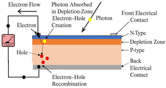
Figure 1. PV cell’s photoelectric effect [23].

When sunlight strikes the PV cell, photons excite electrons in the semiconductor material, generating electricity. A single-junction silicon PV cell typically produces a low voltage, ranging from 0.5 V to 0.6 V under Standard Test Conditions (STCs) [22,23].

To meet practical energy demands, PV cells are arranged into modules or panels, which combine cells in series and parallel configurations. This arrangement increases both the voltage and current output to levels sufficient for residential, commercial, or industrial applications.

2.1. Characteristics of the PV Generator

Manufacturers typically provide the electrical characteristics of PV modules under Standard Test Conditions (STCs). These circumstances are referred to as the surrounding temperature ${\mathrm{T}}_{\mathrm{S}\mathrm{T}\mathrm{C}}=25 °\mathrm{C}$, irradiance value ${\mathrm{G}}_{\mathrm{S}\mathrm{T}\mathrm{C}}=1000 \mathrm{W}/{\mathrm{m}}^2$, and the air mass value AM = 1.5 [22]. Nevertheless, in real-world applications, PV modules function under varying temperature levels and generally smaller irradiance levels. To calculate the output power of a PV module under these conditions, the expected operating temperature must first be determined.

The Nominal Operating Cell Temperature (NOCT) is the level that causes cells to act as open circuits in a PV panel under the following standardized conditions: wind speed = 1 m/s, air temperature ${\mathrm{T}}_{\mathrm{a}\mathrm{m}\mathrm{b}\mathrm{i}\mathrm{a}\mathrm{n}\mathrm{t}}$ = 20 °C, and solar irradiance G = 800 w/${\mathrm{m}}^2$.

Once the NOCT is known, the cell temperature (${\mathrm{T}}_{\mathrm{c}\mathrm{e}\mathrm{l}\mathrm{l}}$) under specific operating conditions can be calculated using the formula [22]

$${\mathrm{T}}_{\mathrm{c}\mathrm{e}\mathrm{l}\mathrm{l}}={\mathrm{T}}_{\mathrm{a}\mathrm{m}\mathrm{b}\mathrm{i}\mathrm{a}\mathrm{n}\mathrm{t}}+\left({\displaystyle \frac{\mathrm{N}\mathrm{O}\mathrm{C}\mathrm{T}-20}{800}}\right)\ast \mathrm{G}$$

(1)

As shown in Figure 2 [23], the three significant points characterizing a PV generator are the maximum power point (MPP) (${\mathrm{V}}_{\mathrm{m}\mathrm{p}\mathrm{p}}$, ${\mathrm{I}}_{\mathrm{m}\mathrm{p}\mathrm{p}}$), the open-circuit voltage (V_oc, 0), and the short-circuit current (0, I_sc).

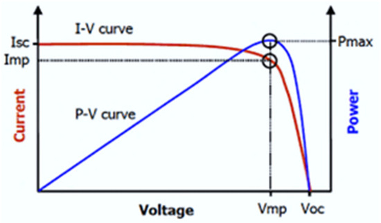
Figure 2. Standard I-V and P-V variations [23].

• The short-circuit current (I_sc) represents the maximum current produced when the generator’s terminals are short-circuited;
• The open-circuit voltage (V_oc) is the maximum voltage generated when the circuit is open (i.e., no current flows);
• The maximum power point (MPP) is the point on the PV generator’s I-V curve where the output power is maximized. It occurs at the bend of the curve, with V_mpp and I_mpp as the corresponding voltage and current, respectively.

Table 1 presents the key specifications of the PV panels used in this work [7].

Table 1. PV panels specifications [7].

Specification	STM6-40/36	STP6-120/36
Manufacturer	Anhui Schutten Solar Energy Co., Ltd.	Anhui Schutten Solar Energy Co., Ltd.
Model Number	STM6-40/36	STP6-120/36
Cell Type	Monocrystalline Silicon	Polycrystalline Silicon
Number of Cells	36	36
Open Circuit Voltage (Voc)	21.02 V	19.21 V
Short Circuit Current (Isc)	1.663 A	7.48 A
Voltage at Pmax (Vmp)	16.98 V	14.93 V
Current at Pmax (Imp)	1.50 A	6.83 A
Temperature [°C]	51	55

2.2. Lumped-Parameter Model of PV Cell

Electrical equivalent circuits are essential for analyzing the characteristics of a photovoltaic (PV) generator. Mathematical models have been developed to better understand and study the effects of varying weather conditions on the electrical output of PV systems. Among these models, which are categorized according to the number of diodes, the lumped parameter model is extensively deployed and has confirmed its effectiveness.

2.3. The One-Diode Model

The one-diode model (ODM), presented in Figure 3, is a popular lumped-parameter model that uses five key electrical parameters:

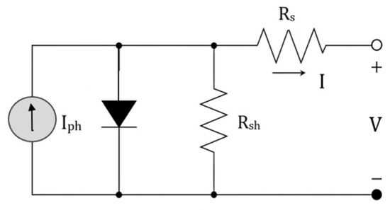
Figure 3. PV cell’s one-diode model [23].

• Photocurrent (I_ph) (in amperes, A): The current generated by the PV cell due to incident sunlight;
• Diode ideality factor (n): The quality of the diode and its deviation from ideal behavior;
• Reverse saturation current (I_s) (often in micro-amperes, $\mathrm{\mu }\mathrm{A}$): A small current that flows through the diode in reverse bias due to thermal generation of carriers;
• Shunt resistance (R_sh) (in ohms, $\mathrm{\Omega }$): Accounts for leakage currents across the PV cell, influencing the cell’s efficiency;
• Series resistance (R_s) (in ohms, $\mathrm{\Omega }$): Represents resistive losses in the cell and interconnections, reducing the output voltage.

The ODM strikes a balance between simplicity and accuracy, making it suitable for modeling PV systems with minimal computational complexity while maintaining high precision.

The one-diode model is represented mathematically as [6,22]

$$\mathrm{I}={\mathrm{I}}_{\mathrm{p}\mathrm{h}}-{\mathrm{I}}_{\mathrm{s}}\left.\left[{\mathrm{e}}^{\left(\left.{\displaystyle \frac{\mathrm{V}+\mathrm{I}\ast {\mathrm{R}}_{\mathrm{s}}}{\mathrm{n}\ast {\mathrm{V}}_{\mathrm{t}}}}\right)\right.}\right.-1\right]-{\displaystyle \frac{\mathrm{V}+\mathrm{I}\ast {\mathrm{R}}_{\mathrm{s}}}{{\mathrm{R}}_{\mathrm{s}\mathrm{h}}}}$$

(2)

where V_t is the thermal voltage.

The one-diode model (ODM) incorporates various features of solar cells, including R_s and R_sh. The series resistance (R_s) accounts for voltage drops and internal losses caused by current flow, while the shunt resistance (R_sh) represents leakage currents to the ground, especially when the diode is reverse-biased. Despite its simplicity, the ODM turns out not to be the best exact representation because it neglects the impact of recombination within the diode [15]. As the number of diodes in a model increases, the accuracy of the PV cell representation improves, albeit at the cost of increased mathematical complexity.

3. PV Panels Parameter Extraction via Optimization Techniques

3.1. Techniques of Optimization

The lumped model equations of PV cells are inherently nonlinear, reflecting the complex relationship between current and voltage. Solving these equations analytically can be challenging due to the nonlinear dependencies and the influence of environmental factors. As a result, scientists have developed a range of optimization techniques, including metaheuristic algorithms, to estimate PV cell parameters effectively.

Metaheuristic optimization algorithms are designed to explore a vast solution space efficiently, identifying high-quality solutions with minimal computational effort. These algorithms are inspired by natural processes, such as the behavior of animals, genetic evolution, and swarm intelligence, and are particularly well suited for problems involving nonlinearity and multiple local optima. Examples include Grey Wolf Optimization Technique (GWO), Particle Swarm Optimization (PSO), Cuckoo Search Algorithm (CSA), Artificial Bee Colony (ABC), the Killer Whale Optimization (KWO) technique, and newer approaches such as the musical chairs algorithm (MCA) [24].

The following nature-inspired optimization algorithms are selected for comparison in this work due to their proven ability to handle complex, nonlinear optimization problems with high accuracy, robustness, and adaptability, which are critical qualities in addressing the complexities and uncertainties of photovoltaic (PV) modeling:

-

Killer Whale Optimization (KWO): This algorithm leverages the cooperative behavior of killer whales to achieve a strong global search capability and effectively balance between exploration and exploitation [20].

-

Improved Opposition-Based Particle Swarm Optimization (IOB-PSO): This enhances convergence and diversity with opposition-based learning, making it well suited for dynamic PV environments [10].

-

Improved Cuckoo Search Algorithm (ImCSA): This incorporates adaptive strategies to improve exploration and prevent premature convergence to local optima [7].

-

Chaotic Improved Artificial Bee Colony (CIABC): This integrates chaotic initialization and convergence stability mechanisms to improve accuracy and reliability in PV parameter estimation [8].

These algorithms have demonstrated superior performance in optimizing nonlinear systems, achieving computational efficiency, and ensuring robust convergence behavior—factors that underscore their suitability for real-world PV modeling applications [7,8,10,20].

3.2. Modified Quasi-Opposition-Based Killer Whale Optimization Technique

3.2.1. Killer Whale Optimization (KWO)

The Killer Whale Optimization (KWO) algorithm draws inspiration from the social structure and hunting strategies of killer whales (Orcinus Orca), which are apex predators in marine ecosystems. Killer whales exhibit three morphological body types—Type A, Type B, and Type C—with Type A being the largest. They are classified into two hunting specializations [20]:

• Mammal-Hunting Transients: These whales migrate with their prey, adapting their hunting strategies to follow seasonal movements;
• Fish-Feeding Residents: These whales remain in fixed regions, relying on predictable patterns to locate and capture fish.

Killer whales use echolocation, producing three main types of vocalizations—clicks, whistles, and pulsed calls—to scan and locate prey. The KWO algorithm mimics these behaviors, integrating the coordination, adaptability, and precision of killer whale hunting strategies into an optimization framework [20].

The hunting pattern is implemented depending on the localization of the killer whale [25] in the mathematical representation. As such, a group of killer whales, guided by a leader that selects the prey and the suitable trajectory to pursue it, is used as search movement-agents to obtain the fittest member and carry the hunting, Figure 4 represents the killer whale foraging geometry where ${\mathrm{d}}_{\mathrm{o}}$ and ${\mathrm{d}}_{\mathrm{F}}$ are the depth of the killer whale and the prey, respectively, and R is the slant range between them, X is the horizontal interval, and θ is the angle that the slant and horizontal range make [20]. Using Equation (3), the angle θ may be computed.

$$\mathsf{\theta }={\sin }^{-1}({\displaystyle \frac{{\mathrm{d}}_{\mathrm{F}}-{\mathrm{d}}_{\mathrm{o}}}{\mathrm{R}}})={\tan }^{-1}({\displaystyle \frac{{\mathrm{d}}_{\mathrm{F}}-{\mathrm{d}}_{\mathrm{o}}}{\mathrm{X}}})$$

(3)

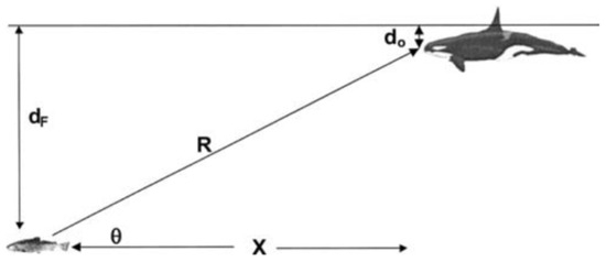
Figure 4. Killer whale’s foraging geometry [20,25].

Each search agent moves from a recent position to a prey location following Equation (4) to calculate velocity of movement and then (5) to find the new position.

$${\mathrm{v}}_{\mathrm{n}+1}^{\mathrm{i}}=\mathrm{w}{\mathrm{v}}_{\mathrm{n}}^{\mathrm{i}}+{\mathrm{c}}_1{\mathrm{r}}_1\left[{\mathrm{p}}_{\mathrm{n}}^{\mathrm{i}}-{\mathrm{x}}_{\mathrm{n}}^{\mathrm{i}}\right]+{\mathrm{c}}_2{\mathrm{r}}_2\left[{\mathrm{p}}_{\mathrm{n}}^{\mathrm{g}}-{\mathrm{x}}_{\mathrm{n}}^{\mathrm{i}}\right]{+\mathrm{c}}_3{\mathrm{r}}_3{\mathrm{l}}_{\mathrm{n}}^{\mathrm{t}}$$

(4)

$${\mathrm{x}}_{\mathrm{n}+1}^{\mathrm{i}}={\mathrm{x}}_{\mathrm{n}}^{\mathrm{i}}+{\mathrm{v}}_{\mathrm{n}+1}^{\mathrm{i}}$$

(5)

$\mathrm{w}$ is the whale inertia;

${\mathrm{c}}_1$ is the personal learning coefficient;

${\mathrm{c}}_2$ is the global leaning coefficient;

${\mathrm{c}}_3$ is the leader influence coefficient;

${\mathrm{r}}_1$, ${\mathrm{r}}_2$, ${\mathrm{r}}_3$ are random numbers between 0 and 1;

${\mathrm{p}}^{\mathrm{i}}$ is whale’s best-known position;

${\mathrm{l}}^{\mathrm{t}}$ is the ${\mathrm{t}}^{\mathrm{t}\mathrm{h}}$ leader position;

${\mathrm{p}}^{\mathrm{g}}$ is the global best position;

${\mathrm{x}}^{\mathrm{i}}$ is the ${\mathrm{i}}^{\mathrm{t}\mathrm{h}}$ element position in the solution interval.;

${\mathrm{v}}^{\mathrm{i}}$ is the ${\mathrm{i}}^{\mathrm{t}\mathrm{h}}$ whale speed.

The interval of a fitness function is searched by the modified KWO technique by adjusting the trajectories of individual search agents. The “t” Matrilines of these whales travel across the search space while each group is guided by a leader. Each agent i has a tendency to wander randomly but is also attracted to the present position overall best g* and its own best position ${\mathrm{x}}^{\mathrm{i}}$. So far, it is influenced by the current leader’s position l. The agents are first random arranged in the solution interval. The fitness value is computed for all the members; As a member i falls on a position that is better than the so far found positions, it records it to be the updated present best ${\mathrm{x}}^{\mathrm{i}}$ through revising speed using Equation (4) based on movement inertia, personal, leader, and global learning coefficients and then using Equation (5) to update its position at each iteration. Thus, at any time t during the iterations, a present leading position would exist for all n whales. The objective is to identify the overall finest member among all the obtained utmost members till the fitness function does not vary much or after a predetermined number of repetitions.

In this optimization technique, the optimum direction is defined by the minimum direction and maximum velocity. If the group’s leader fitness value is smaller than the current global best cost, the group members follow their leader’s position, and the Global best position is updated. Otherwise, they follow the current global best position.

3.2.2. Cluster for Search Space

The proposed algorithm is designed for solving very complex optimization problems with many variables. It has a memorize capability for each matriline, which will affect the time consumption to solve the problem due to its complexity; however, the required number of iterations in this technique is small.

The idea behind the Killer Whale technique as a collection of members is that the space of optimization can be clustered using Hartigan and Wong’s Method [26]. The leader and members trace the search area of each cluster, and the search starts at the centroid of each cluster. Each killer whale will aim to find a neighboring best solution inside a subset from the set’s centroid. Centers are updated considering each point, rather than after each pass over the entire data set. This technique is used to achieve the best overall solution of the fitness function faster by avoiding falling into the local optimum value. The clustering process necessitates matrix entry of Npop points and Nleaders original cluster centers in D dimensions. The number of points in a cluster Team is labeled as NC (Team), D (I, Team) is the distance between point I and cluster Team, the typical process consists of looking for an Nleaders-division having locally best within-cluster addition of squares through shifting points from either set to the other.

3.2.3. Quasi-Opposition-Based Learning (QOBL)

Quasi-Oppositional-Based Learning (QOBL) is an enhancement mechanism used in optimization algorithms to improve the diversity of the population while maintaining convergence efficiency. By introducing quasi-opposite solutions and selecting the best candidates, this process results in better exploration of the search space and improved optimization performance, as detailed in [18].

Unlike traditional opposition-based learning (OBL), which generates a direct opposite candidate solution in the search space, QOBL generates a quasi-opposite solution using the opposite solution as defined in Equations (6) and (7) [18]. This quasi-opposite lies between the current solution and its opposite, rather than being at the extreme boundary. The idea is to increase the population uniformity by providing more refined, potentially better candidate solutions during the early and middle stages of the search process, reducing the risk of premature convergence while maintaining exploration efficiency. QOBL is especially useful in complex, multimodal optimization problems where maintaining a balance between exploration and exploitation is critical. This approach involves the following steps [18]:

• Dual Initialization: Both the population and its quasi-opposite population are initialized simultaneously;
• Fitness Evaluation: The fitness function is evaluated for both populations to assess the quality of each solution;
• Selection of Fittest Solutions: Only the fittest solutions from both populations are retained to form the new population.
  Particle, a member of the population ${\mathrm{p}}^{\mathrm{i}}$, is written as
  ${\mathrm{p}}^{\mathrm{i}}$ Є [a, b] such that, i = 1, 2,…, D and a, b є R;
  D denotes dimensions, and R designates real numbers;
  Opposite particle: each member ${\mathrm{p}}^{\mathrm{i}}$ has a single opposed ${{\mathrm{p}}^{\mathrm{i}}}_{\mathrm{o}\mathrm{p}}$ written as

$${{\mathrm{p}}^{\mathrm{i}}}_{\mathrm{O}\mathrm{P}}=\mathrm{a}+\mathrm{b}-{\mathrm{p}}^{\mathrm{i}}$$

(6)

Such that, i = 1, 2,…D and a, b є R

$$\mathrm{If} {\mathrm{p}}^{\mathrm{i}}<{\displaystyle \frac{\mathrm{a}+\mathrm{b}}{2}}\mathrm{then} {\mathrm{p}}_{\mathrm{Q}\mathrm{B}\mathrm{L}}^{\mathrm{i}}={\displaystyle \frac{\mathrm{a}+\mathrm{b}}{2}}+({{\mathrm{p}}^{\mathrm{i}}}_{\mathrm{O}\mathrm{P}}-{\displaystyle \frac{\mathrm{a}+\mathrm{b}}{2}}).\mathrm{r}\mathrm{a}\mathrm{n}\mathrm{d}(\mathrm{D})$$

(7)

$$\mathrm{Else} {\mathrm{p}}_{\mathrm{Q}\mathrm{B}\mathrm{L}}^{\mathrm{i}}={{\mathrm{p}}^{\mathrm{i}}}_{\mathrm{O}\mathrm{P}}+({\displaystyle \frac{\mathrm{a}+\mathrm{b}}{2}}-{{\mathrm{p}}^{\mathrm{i}}}_{\mathrm{O}\mathrm{P}}).\mathrm{r}\mathrm{a}\mathrm{n}\mathrm{d}(\mathrm{D})$$

3.2.4. Quasi-Opposition-Based Killer Whale Optimization (QOB-KWO)

To enhance the performance of the Killer Whale Optimization (KWO) algorithm, a novel integration of the Quasi-Opposition-Based Learning (QOBL) mechanism is proposed. This modification introduces a new level of adaptability by leveraging quasi-opposite solutions to improve both the exploration and exploitation capabilities during the search process. Unlike traditional KWO, the inclusion of QOBL diversifies the search space more effectively and helps prevent premature convergence by reducing the risk of becoming trapped in local optima. Such enhancements are particularly beneficial for complex, nonlinear optimization problems such as photovoltaic (PV) parameter identification, where precision and convergence speed are critical.

In this algorithm, the QOBL is integrated in two stages:

• The initialization stage (Quasi Opposition-Based Initialization): This step aims to achieve fitter starting candidate solutions and enhance the initial leader selection. By generating quasi-opposite solutions in this early phase, the algorithm increases the likelihood of starting closer to the global optimum. Key parameters determined during this stage include the following:
  • Number of Matrilines and leaders in the population;
  • Dimensions of the objective function;
  • Global optimum estimation;
  • Lower and upper bounds of the optimized variables;
  • Number of clusters;
  • Number of iterations for the clustering process.
• The KWO main loop (Quasi-Opposition-Based Generation Jumping): During the main iteration process, QOBL is employed to force the current population to jump into some new candidate solutions, which ideally are fitter than the current ones. This “generation jumping” strategy encourages the algorithm to escape potential stagnation zones and explore new, potentially fitter regions of the search space.

By embedding QOBL into both the initialization and iterative phases of KWO, a novel and effective framework for improving convergence and solution quality is introduced. The strategic use of QOBL not only strengthens the global search ability but also ensures that the algorithm remains robust across various complex and multimodal optimization landscapes.

3.3. Lumped Model Parameters Extraction Using a Modified QOB-KWO

The following objective function is used for the one-diode model:

$$\left\{\begin{array}{c}F(x)=I-{\mathrm{I}}_{\mathrm{p}\mathrm{h}}-{\mathrm{I}}_{\mathrm{s}}\left.\left[{\mathrm{e}}^{\left(\left.{\displaystyle \frac{\mathrm{V}+\mathrm{I}\ast {\mathrm{R}}_{\mathrm{s}}}{\mathrm{n}\ast {\mathrm{N}}_{\mathrm{s}}\ast {\mathrm{V}}_{\mathrm{t}}}}\right)\right.}\right.-1\right]-{\displaystyle \frac{\mathrm{V}+\mathrm{I}\ast {\mathrm{R}}_{\mathrm{s}}}{{\mathrm{R}}_{\mathrm{s}\mathrm{h}}}}\\ x=\left\{{{\mathrm{I}}_{\mathrm{p}\mathrm{h}},\mathrm{I}}_{\mathrm{s}},{\mathrm{R}}_{\mathrm{s}},\mathrm{n},\right.\left.{\mathrm{R}}_{\mathrm{s}\mathrm{h}}\right\}\end{array}\right.$$

(8)

The fitness function to be minimized by this algorithm accounts for the error between the measurements and model-based simulated data. It is selected to be the Root Mean Square Error (RMSE) that is widely used by researchers to solve the photovoltaic model’s parameters estimation [7,8,27,28], due to its good alignment with curve fitting objectives, especially around the nonlinear regions. The RMSE is defined by

$$\mathrm{R}\mathrm{M}\mathrm{S}\mathrm{E}=\sqrt{{\displaystyle \frac{1}{\mathrm{N}}}\sum _1^{\mathrm{N}}{\mathrm{F}\left(\mathrm{x}\right)}^2}$$

(9)

3.4. Algorithm Hyperparameter Tuning

The hyperparameter tuning of the modified QOB-KWO was performed manually based on the algorithm’s inspiration: the killer whale hunting mechanism, which states that the search agents are clustered into groups guided by a leader whale. The whales explore the search space, following a foraging geometry sketch by a leader [20]. Through iterations, the best leader is updated to be selected as the global best. Depending on this process, the MQOB-KWO control parameters were tuned manually through several trials to result in the given results presented in Table 2. A reduction on the cognitive factor that is the personal learning coefficient was suggested as c1 = 0.5 to limit self-exploration. For the social factor c2 = 2, the same value as in the original algorithm KWO [20,29,30,31] is maintained to keep a strong group influence. The leader factor is set at a value of c3 = 0.9 to ensure a high reliance on the best solution [32]. Moreover, an adaptive damping ratio w varying from 0.2 to 0.9 was exploited [10,29,31] so the algorithm can exhibit a transition from high exploration to strong exploitation. Furthermore, the application of the Quasi-Opposition-Based Learning (QOBL) on the population initialization, initial leader selection establishes a better diversity and faster convergence since the initialized population is already well selected and distributed, and in the main KWO loop, the periodically introduced quasi-opposite solutions result in exploration enhancement and prevents stagnation by keeping the search dynamic and avoiding early trapping in local optima.

Table 2. MQOB-KWO parameters.

Algorithm Parameters	Selected Value	Description	Justification
Cognitive Factor c1	0.5	Controls personal learning or self-exploration	Since QOBL enhances diversity, c1 is reduced to limit excessive randomness and self-exploration [29,30,31].
Social Factor c2	2	Governs social learning or group influence	To preserve strong group guidance and alignment with biological inspiration, c2 is maintained as in the original KWO [20].
Leader Factor c3	0.9	Determines the influence of the best leader	This value ensures strong convergence toward the global best [32], balanced by QOBL to avoid premature convergence.
Damping Ratio (inertia weight) w	0.2–0.9 (Adaptive)	Controls the trade-off between exploration and exploitation across iterations	Adaptive scheme: high w at start encourages exploration; low w at end supports exploitation [10,29,31]. QOBL counteracts excessive convergence
No. of whales	80	Number of members in the population.	Empirically chosen to ensure sufficient diversity while maintaining reasonable computational cost.
Maximum Iteration	80	Total number of optimization cycles.	Provides a balanced trade-off between solution quality and computational time for typical PV parameter estimation problems.

The combination of QOBL and the previous selection of the hyperparameters can be justified as QOBL enhancing the exploration; thus, a lower c1 = 0.5 stabilizes the search space without excessive randomness. The dynamic providing of better solutions by the QOBL in the main KWO loop helps avoid a premature convergence that can be due to the high dependence on the best solution; thus, it balances the setting of the leader factor c3 = 0.9. Finally, the use of an adaptive damping ratio (w = 0.2 to 0.9) balances the exploration in the early stage (w ≈ 0.9), and the exploitation in a later stage (w ≈ 0.2), where the QOBL counteracts excessive exploitation and maintains diversity even when w is low.

To conclude, the proposed parameters tuning combined with the QOBL process results in the following:

• An improved exploration without losing efficiency (QOBL enhances exploration, reducing the need for a high c1).
• Faster convergence with reduced risk of premature convergence (a strong initial population and continuous improvement are confirmed due to the combination of QOBL and adaptive damping).
• Better balance between exploration and exploitation (early exploration is improved by high w and QOBL, while later exploitation is ensured by strong leader pursuing (c3 = 0.9)).

Table 2 summarizes the selected parameter combinations with the QOB-KWO process [10,20,29,30,31,32].

The Flowchart of the MQOB-KWO is illustrated in Figure 5, and its pseudo code in Algorithm 1.

Algorithm 1: Pseudo code of the modified QOB-KWO

1. Initialize the killer whale population 2. Create a quasi-opposition based killer whale population 3. Compute fitness value for both populations 4. Create a new population using only the fittest particles from both populations 5. Initially select leaders 6. Find the quasi opposite leaders 7. Compute fitness value for all leaders 8. Select the fittest leaders 9. for It = 1: Itmax 10. Whales population is clustered into groups, each group is guided by a leader 11. All search agents including leaders search for a prey 12. Leader of Matriline decides the potential prey to chase 13. Apply quasi opposition based learning 14. Leader scan for another potential prey 15. All members chase the prey depending on the leader’s decision 16. Matriline create search pattern for the prey 17. If (new potential prey < chased prey) then 18. Move to chase the new potential prey 19. Else Keep chasing old potential prey 20. End If 21. End for 22. Matriline memorize pattern of prey 23. Determine the global optimum value 24. End procedure

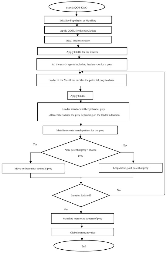
Figure 5. Flowchart of the modified QOB-KWO.

4. Results and Discussion

The modified QOB-KWO algorithm is used for ODM parameter identification using the curve fitting tool. The technique is applied to two PV panels and contrasted with other methods to demonstrate its reliability. It is coded in MATLAB R2021a and run on a PC with Intel (R) Core (TM) i5-8365U CPU @ 1.60GHz 1.90 GHz, 8GB RAM, under Windows 11 64-bit OS. Table 3 presents the search ranges used for the parameters’ optimization [9,10,33].

Table 3. ODM parameter search ranges.

Parameter	Search Range
${\mathrm{I}}_{\mathrm{p}\mathrm{h}}$	[0.95 × ${\mathrm{I}}_{\mathrm{s}\mathrm{c}}$, 1.05 × ${\mathrm{I}}_{\mathrm{s}\mathrm{c}}$]
${\mathrm{I}}_{\mathrm{s}}$	[1µA, 5 µA]
$\mathrm{n}$	[1,2]
${\mathrm{R}}_{\mathrm{s}\mathrm{h}}$	[${\displaystyle \frac{{\mathrm{V}}_{\mathrm{m}\mathrm{p}\mathrm{p}}}{{\mathrm{I}}_{\mathrm{s}\mathrm{c}}-{\mathrm{I}}_{\mathrm{m}\mathrm{p}\mathrm{p}}}}$, 1500 Ω]
${\mathrm{R}}_{\mathrm{s}}$	[0, ${\displaystyle \frac{{\mathrm{V}}_{\mathrm{m}\mathrm{p}\mathrm{p}}-{\mathrm{V}}_{\mathrm{o}\mathrm{c}}}{{\mathrm{I}}_{\mathrm{m}\mathrm{p}\mathrm{p}}}}$]

The MQOB-KWO is deployed to identify model parameters for the different photovoltaic modules presented in Table 4.

Table 4. The utilized photovoltaic modules.

Module	Type	${\mathbf{N}}_{\mathbf{s}}$	Temperature [°C]	$\mathbf{Irradiance} [\mathbf{W}/{\mathbf{m}}^2]$
STM6-40/36	Monocrystalline	36	51	NA
STP6-120/36	Polycrystalline	36	55	NA

NA: not available.

4.1. Simulation Results and Discussion

The I-V experimental data [7] that were acquired for the monocrystalline STM6-40/36 panel at a temperature of T = 51 °C, in addition to I-V data that were measured at T = 55 °C [7] for the STP6-120/36 multicrystalline panel, are processed in the modified QOB-KWO to test their efficiency. The outcomes of the study are reported in Table 5, Table 6, Table 7 and Table 8 such that Table 5 and Table 7 present the results obtained compared to previously published algorithms’ findings. Table 6 and Table 8 compare the integral absolute error (IAE) between the experimental real current values and the calculated current using the estimated ODM parameters obtained by the enhanced and the original KWO algorithm.

Table 5. Comparison among PV panel (STM6-40/36) estimated parameters achieved by different methods.

Meth.	Parameters					Error
	${\mathbf{I}}_{\mathbf{p}\mathbf{h}}\left[\mathbf{A}\right]$	${\mathbf{I}}_{\mathbf{s}}\left[\mathbf{\mu }\mathbf{A}\right]$	N	${\mathbf{R}}_{\mathbf{s}}\left[\mathbf{\Omega }\right]$	${\mathbf{R}}_{\mathbf{s}\mathbf{h}}\left[\mathbf{\Omega }\right]$	RMSE
CIABC [8]	1.664	1.676	1.498	4.400	15.617	1.819 × 10−3
ImCSA [7]	1.664	2.000	1.533	2.914	15.841	1.795 × 10−3
IOB-PSO [10]	1.663	2.884	1.570	1.5 × 10−3	598.735	1.7723 × 10−3
KWO	1.663	2.529	1.560	3.987 × 10−2	591.080	1.7761 × 10−3
MQOB-KWO *	1.663	2.886	1.570	1.412 × 10−3	599.026	1.7723 × 10−3

* Proposed method.

Table 6. The calculated results of the proposed MQOB-KWO and the original KWO for the ODM of the (STM6-40/36) monocrystalline panel.

Item	Experimental Data		MQOB-KWO		KWO
	V (V)	I (A)	${\mathbf{I}}_{\mathbf{c}\mathbf{a}\mathbf{l}}$ (A)	IAE	${\mathbf{I}}_{\mathbf{c}\mathbf{a}\mathbf{l}}$ (A)	IAE
1	0.118	1.663	1.66299	0.00001	1.662881	0.000118
2	2.237	1.661	1.662883	0.001883	1.662774	0.001773
3	5.434	1.653	1.662656	0.009656	1.662551	0.00955
4	7.26	1.65	1.662376	0.012376	1.66228	0.01228
5	9.68	1.645	1.661227	0.016227	1.66118	0.01618
6	11.59	1.64	1.658032	0.018032	1.658109	0.018109
7	12.6	1.636	1.654022	0.018022	1.654238	0.018238
8	13.37	1.629	1.648716	0.019716	1.649102	0.020102
9	14.09	1.619	1.640797	0.021797	1.641416	0.022416
10	14.88	1.597	1.626785	0.029785	1.627781	0.03078
11	15.59	1.581	1.606602	0.025602	1.608101	0.027101
12	16.4	1.542	1.568928	0.026928	1.571652	0.029652
13	16.71	1.524	1.549129	0.025129	1.551946	0.027946
14	16.98	1.5	1.528046	0.028046	1.531332	0.031331
15	17.13	1.485	1.514681	0.029681	1.518265	0.033264
16	17.32	1.465	1.495826	0.030826	1.499831	0.03483
17	17.91	1.388	1.420512	0.032512	1.426243	0.038243
18	19.08	1.118	1.155525	0.037525	1.168442	0.050441
Sum of IAE				0.383753		0.422362

Table 7. Comparison among PV panel (STP6-120/36) estimated parameters achieved by different methods.

Meth.	Parameters					Error
	${\mathbf{I}}_{\mathbf{p}\mathbf{h}}\left[\mathbf{A}\right]$	${\mathbf{I}}_{\mathbf{s}}\left[\mathbf{\mu }\mathbf{A}\right]$	n	${\mathbf{R}}_{\mathbf{s}}\left[\mathbf{\Omega }\right]$	${\mathbf{R}}_{\mathbf{s}\mathbf{h}}\left[\mathbf{\Omega }\right]$	RMSE
CIABC [8]	7.4841	1.29	1.2149	5.1000	9.89	1.6286 × 10−2
ImCSA [7]	7.4827	1.00	1.1977	5.3869	10.00	1.5865 × 10−2
IOB-PSO [10]	7.4570	1.28	1.2200	0.1882	1499.84	1.5654 × 10−2
KWO	7.4570	1.31	1.2200	0.1872	1481.56	1.5697 × 10−2
MQOB-KWO *	7.4600	1.44	1.2200	0.1766	1499.58	1.4124 × 10−2

* Proposed method.

Table 8. The calculated results of the proposed MQOB-KWO and the original KWO for the ODM of the (STP6-120/36) multicrystalline panel.

Item	Experimental Data		MQOB-KWO		KWO
	V (V)	I (A)	${\mathbf{I}}_{\mathbf{c}\mathbf{a}\mathbf{l}}$ (A)	IAE	${\mathbf{I}}_{\mathbf{c}\mathbf{a}\mathbf{l}}$ (A)	IAE
1	17.65	3.83	3.822788	0.007212	3.964621	0.134621
2	17.41	4.29	4.266257	0.023742	4.388067	0.098067
3	17.25	4.56	4.540371	0.019628	4.650033	0.090033
4	17.1	4.79	4.781844	0.008155	4.880965	0.090964
5	16.9	5.07	5.080803	0.010803	5.167098	0.097097
6	16.76	5.27	5.274742	0.004742	5.352861	0.082861
7	16.34	5.75	5.784055	0.034055	5.841305	0.091305
8	16.08	6	6.048192	0.048192	6.095004	0.095004
9	15.71	6.36	6.363382	0.003381	6.398129	0.038128
10	15.39	6.58	6.584936	0.004935	6.611483	0.031482
11	14.93	6.83	6.833544	0.003543	6.851195	0.021194
12	14.58	6.97	6.977264	0.007264	6.989932	0.019931
13	14.17	7.1	7.106175	0.006175	7.114481	0.014481
14	13.59	7.23	7.233647	0.003646	7.237744	0.007743
15	13.16	7.29	7.298052	0.008052	7.300064	0.010063
16	12.74	7.34	7.34343	0.003429	7.34399	0.003989
17	12.36	7.37	7.373483	0.003483	7.37309	0.00309
18	11.81	7.38	7.403794	0.023794	7.402447	0.022447
19	11.17	7.41	7.425879	0.015879	7.423841	0.013841
20	10.32	7.44	7.442219	0.002218	7.439672	0.000328
21	9.74	7.42	7.448452	0.028451	7.445712	0.025712
22	9.06	7.45	7.452881	0.00288	7.450003	0.000003
Sum of IAE				0.273669		0.992393

The photovoltaic characteristics of these panels are simulated using the obtained ODM parameters by the MQOB-KWO and contrasted with the utilized experimental data in Figure 6 and Figure 7.

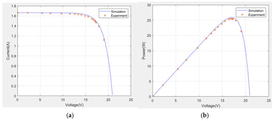
Figure 6. Contrasting (a) I-V and (b) P-V measurements with the ODM (STM6-40/36 PV panel).

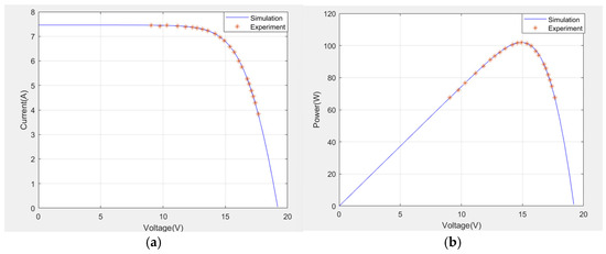
Figure 7. Contrasting (a) I-V and (b) P-V measurements with the ODM (STP6-120/36 module PV panel).

The Modified Quasi-Opposition-Based Killer Whale Optimization (MQOB-KWO) algorithm demonstrates significant potential for accurately identifying photovoltaic (PV) parameters. This algorithm was evaluated using experimental I-V data using the STM6-40/36 (monocrystalline) and the STP6-120/36 (polycrystalline), under varying environmental conditions. The experimental results validate its effectiveness, showcasing its robustness and efficiency. From Table 5 and Table 7, the MQOB-KWO algorithm achieved consistently lower Root Mean Square Error (RMSE) values compared to other optimization methods, such as CIABC, ImCSA, and IOB-PSO and the original KWO. For the STM6-40/36 module, the RMSE was 1.7723 × 10⁻³, and for the STP6-120/36 module, it was 1.4124 × 10⁻². Additionally, based on the comparison results of the MQOB-KWO with the original KWO according to the integral absolute error IAE between the calculated current using the estimated parameters, and the experimental real current values, given in Table 6 and Table 8. It can be observed that the MQOB-KWO has better values in terms of IAE. These results highlight the algorithm’s ability to closely approximate the experimental data and minimize errors. Moreover, the I-V and P-V measured data points compared to the simulated graphs of the STM6-40/36 and the STP6-120/36 modules that are given in Figure 6 and Figure 7 reveal an agreement between the experimental data and the simulated characteristics. Thus, it can be claimed that this technique has good accuracy and is reliable for extracting the PV parameters.

Convergence was another major advantage observed with MQOB-KWO. For the STM6-40/36 module (18 pairs of current/voltage data), the algorithm’s total processing time is 47.42 s (80 iterations), while for the STP6-120/36 module (22 pairs of current-voltage data), the total time needed to complete the total number of iterations (80 iterations) is 64.86 s. As presented in Figure 8, the MQOB-KWO demonstrated good convergence speed, making it well suited for real-time or large-scale PV system parameterization. These results prove that the MQOB-KWO has a good convergence speed and hence the efficiency of using this method to solve complex multivariable problems.

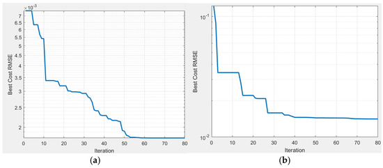
Figure 8. Fitness value progress of the MQOB-KWO for the (a) STM6−40/36 module and (b) STP6−120/36 module.

4.2. Evaluation of Model Fitting Accuracy

In order to evaluate the performance of the proposed MQOB-KWO, a comparative analysis was conducted with the standard KWO algorithm for both tested PV panels. The coefficient of determination (${\mathrm{R}}^2$) was employed to assess the quality of curve fitting between the simulated and experimental I-V data. Table 9 presents the obtained results.

Table 9. Coefficient of determination (${\mathrm{R}}^2$) for the monocrystalline STM6-40/36 and the polycrystalline STP6-120/36 panels using the proposed MQOB-KWO and KWO.

Meth.	Coefficient of Determination $\left({\mathbf{R}}^2\right)$
	STM6−40/36	STP6−120/36
KWO	0.959142	0.997253
MQOB-KWO *	0.967861	0.999782

* Proposed method.

The MQOB-KWO algorithm demonstrated superior performance, achieving an ${\mathrm{R}}^2$ of 0.967861 for the STM6-40/36 and 0.999782 for the STP6-120/36. In contrast, the standard KWO algorithm attained ${\mathrm{R}}^2$ values of 0.959142 and 0.997253 for the same panels, respectively. These findings indicate that the proposed MQOB-KWO is more robust, providing more accurate and reliable parameter estimation for different panel types.

4.3. Results of the Welch’s Two-Sample T-Test

Static verification of the results obtained using MQOB-KWO and the original KWO was performed using Welch’s two-sample t-test for the real data sets of the tested PV panels, the STM6-40/36 and the STP6-120/36 modules. Table 10 and Table 11 show the statistics of the fitness function (RMSE) values for the monocrystalline STM6-40/36 panel and the polycrystalline panel STP6-120/36, respectively, using the proposed MQOB-KWO and the KWO, obtained by executing the algorithms over 40 runs with a similar number of whale population 80 and total iteration number 80 for a fair comparison. The obtained t-value, h-value, CI, and p-value for the t-test are given in Table 12.

Table 10. Statistics of the RMSE values for the monocrystalline STM6−40/36 panel using the proposed MQOB-KWO and KWO.

RMSE	Worst	Median	Best	Mean	Standard Deviation
KWO	2.963 × 10−3	1.835 × 10−3	1.17761 × 10−3	1.915 × 10−3	2.26 × 10−4
MQOB-KWO *	1.951 × 10−3	1.785 × 10−3	1.17723 × 10−3	1.806 × 10−3	4.4 × 10−5

* Proposed method.

Table 11. Statistics of the RMSE values for the polycrystalline STP6−120/36 panel using the proposed MQOB-KWO and KWO.

RMSE	Worst	Median	Best	Mean	Standard Deviation
KWO	1.9932 × 10−2	1.7926 × 10−2	1.5697 × 10−2	1.7771 × 10−2	1.223 × 10−3
MQOB-KWO *	1.8633 × 10−2	1.7335 × 10−2	1.4124× 10−2	1.7168 × 10−2	1.179 × 10−3

* Proposed method.

Table 12. Results of the t-test on the data in Table 10 and Table 11.

PV Panel	t-Value	h-Value	CI	p-Value
STM6-40/36	−2.980195	1	[−0.000182,−0.000035]	0.004700
STP6-120/36	−2.245653	1	[−0.001138,−0.000068]	0.027561

Based on Table 10 and Table 11, it can be seen that the performance of the MQOB-KWO is better than the KWO based on all statistical measures, counting the worst, median, best, mean, and standard deviation of the fitness (RMSE) values in all 40 independent runs for both tested panels STM6-40/36 and STP6-120/36. These results prove that the proposed MQOB-KWO is better than the original KWO, with respect to precision and effectiveness, and enhances the original KWO.

Based on Table 12, the t-values seem to have negative values. This means that the results of the MQOB-KWO are comparatively smaller. The h values, on the other hand, are ones that convey that the performances of both techniques are statistically different at the 0.05 significance level. The confidence interval CI has negative values and does not contain zero, and all the p-values turn out to be less than 0.05. This indicates that the MQOB-KWO performs considerably better than KWO for both PV panels, with respect to statistical significance. Thus, the reliable findings utilizing Welch’s t-test demonstrate that the MQOB-KWO noticeably improves the reliability of conventional KWO.

The improved parameter estimation achieved using the Modified Quasi-Opposition-Based Killer Whale Optimization (MQOKWO) algorithm enhances the accuracy of PV modeling under varying environmental conditions, leading to more precise system design and efficient operation. This contributes to optimal sizing and configuration of system components, including inverters, MPPT controllers, and energy storage units, ensuring both improved MPPT performance and reliable fault detection, and, thus, performance efficiency and cost-effectiveness. As a result, the approach contributes to maximizing energy yield, reducing operational costs, and increasing system reliability and sustainability of PV installations, making it highly beneficial for real-world PV applications, particularly in dynamic environments such as smart grids and hybrid renewable energy systems.

5. Conclusions

This paper proposed an enhanced Killer Whale Optimization (KWO) algorithm, modified using the Quasi-Opposition-Based Learning (QOBL) mechanism to improve its capability in solving complex, multivariable problems. The enhanced algorithm MQOB-KWO was applied to the photovoltaic (PV) parameter extraction problem based on the one-diode model. Experimental real I-V data for two distinct PV modules, measured under varying environmental conditions, were processed to validate the algorithm.

The results of MQOB-KWO were compared with those obtained using other established optimization techniques reported in previous research. The modified QOB-KWO demonstrated good accuracy, achieving the lowest Root Mean Square Error (RMSE) in parameter estimation among the tested methods, and a smaller Integral Absolute Error (IAE) compared to the original KWO. Hence, based on the obtained coefficient of determination (${\mathrm{R}}^2$), the simulated I-V and P-V characteristics generated using the extracted parameters showed strong alignment with experimental data. Moreover, statistical verification using Welch’s t-test performed for the proposed algorithm and the original KWO proved that the MQOB-KWO yields a significant performance enhancement compared to the original KWO. This agreement underscores the reliability of the algorithm in accurately modeling PV systems. Furthermore, its ability to generalize across different module types and environmental conditions enhances its applicability in diverse real-world scenarios.

In addition to its accuracy, the proposed MQOB-KWO exhibited high computational efficiency, requiring less than 65 s to complete the optimization process using the RMSE metric. This computational efficiency, combined with its demonstrated accuracy, establishes the Modified Quasi-Opposition-Based Killer Whale Optimization (MQOB-KWO) technique as a promising tool for PV parameter estimation, particularly for real-time or large-scale PV applications, thus offering a promising solution for the accurate modeling, real-time monitoring, and optimization of advanced photovoltaic systems. This contributes to the advancement of PV technology.

For future research work, the MQOB-KWO algorithm’s adaptability to more complex models, such as the double-diode, three-diode model, and the four-diode model, will be explored and discussed. Additionally, scalability for large PV arrays and performance under extreme environmental variations require further study.

References

- International Energy Agency (IEA). Renewable Energy Market Report 2023. REN21. In Renewables Global Status Report; IEA: Paris, France, 2022. [Google Scholar]
- IEA—International Energy Agency. 2020. Available online: https://www.iea.org/energy-system/renewables/solar-pv (accessed on 20 December 2024).
- Green, M.A.; Dunlop, E.D.; Hohl-Ebinger, J.; Yoshita, M.; Kopidakis, N.; Hao, X. Solar cell efficiency tables (version 64). Prog. Photovolt. Res. Appl. 2024, 32, 3–23. [Google Scholar] [CrossRef]
- Spampinato, C.; La Magna, P.; Valastro, S.; Smecca, E.; Arena, V.; Bongiorno, C.; Mannino, G.; Fazio, E.; Corsaro, C.; Neri, F.; et al. Infiltration of CsPbI3:EuI2 Perovskites into TiO2 Spongy Layers Deposited by gig-lox Sputtering Processes. Solar 2023, 3, 347–361. [Google Scholar] [CrossRef]
- Patel, H.; Agarwal, V. MATLAB-Based Modeling to Study the Effects of Partial Shading on PV Array Characteristics. IEEE Trans. Energy Convers. 2008, 23, 302–310. [Google Scholar] [CrossRef]
- Villalva, M.G.; Gazoli, J.R.; Filho, E.R. Comprehensive Approach to Modeling and Simulation of Photovoltaic Arrays. IEEE Trans. Power Electron. 2009, 24, 1198–1208. [Google Scholar] [CrossRef]
- Kang, T.; Yao, J.; Jin, M.; Yang, S.; Duong, T. A Novel Improved Cuckoo Search Algorithm for Parameter Estimation of Photovoltaic Models. Energies 2018, 11, 1060. [Google Scholar] [CrossRef]
- Oliva, D.; Ewees, A.A.; Aziz, M.A.E.; Hassanien, A.E.; Cisneros, M.P. A Chaotic Improved Artificial Bee Colony for Parameter Estimation of Photovoltaic Cells. Energies 2017, 10, 865. [Google Scholar] [CrossRef]
- Touabi, C.; Bentarzi, H. Photovoltaic Panel Parameters Estimation Using Grey Wolf Optimization Technique. Eng. Proc. 2022, 14, 3. [Google Scholar]
- Touabi, C.; Ouadi, A.; Bentarzi, H. Photovoltaic Panel Parameters Estimation Using an Opposition Based Initialization Particle Swarm Optimization. Eng. Proc. 2023, 3, 16. [Google Scholar]
- Gamgula, B.; Saripalli, B.P. Enhanced dynamic inertia particle swarm optimization with velocity clamping for accurate parameter extraction in one-diode and two-diode solar PV models. World J. Eng. 2025; ahead-of-print. [Google Scholar] [CrossRef]
- Nema, S.; Nema, R.K.; Agnihotri, G. MATLAB/Simulink-Based Study of Photovoltaic Cells/Modules/Array and Their Experimental Verification. Int. J. Energy Environ. 2010, 1, 487–500. [Google Scholar]
- Saripalli, B.P.; Gamgula, B.; Ravilisetty, R.; Kumar, P.; Singh, G.; Singh, S. Advanced parameter extraction optimization technique for the four-diode model approach. e-Prime Adv. Electr. Eng. Electron. Energy 2024, 10, 100861. [Google Scholar] [CrossRef]
- Allouhi, A.; Saadani, R.; Buker, M.; Kousksou, T.; Jamil, A.; Rahmoune, M. Energetic, economic and environmental (3E) analyses and LCOE estimation of three technologies of PV grid-connected systems under different climates. Sol. Energy 2019, 178, 25–36. [Google Scholar] [CrossRef]
- Udoka, E.V.H.; Umaru, K.U.; Edozie, E.; Nafuna, R.; Yudaya, N. The Differences between Single Diode Model and Double Diode Models of a Solar Photovoltaic Cells: Systematic Review. J. Eng. Technol. Appl. Sci. JETAS 2023, 5, 57–66. [Google Scholar] [CrossRef]
- Saripalli, B.P.; Singh, G.; Singh, S. A simplified three-diode model for photovoltaic module: Cell modeling and performance analysis. World J. Eng. 2024, 21, 1173–1182. [Google Scholar] [CrossRef]
- Gandomi, A.H.; Alavi, A.H. Krill Herd: A New Bio-Inspired Optimization Algorithm. Commun. Nonlinear Sci. Numer. Simul. 2012, 17, 4831–4845. [Google Scholar] [CrossRef]
- Kazimipour, B.; Li, X.; Qin, A.K. Initialization methods for large scale global optimization. In Proceedings of the 2013 IEEE Congress on Evolutionary Computation, Cancun, Mexico, 20–23 June 2013; pp. 2750–2757. [Google Scholar]
- Kennedy, J.; Eberhart, R. Particle Swarm Optimization. In Proceedings of the IEEE International Conference on Neural Networks, Perth, WA, Australia, 27 November–1 December 1995. [Google Scholar]
- Biyanto, T.R.; Matradji, B.; Irawan, S.; Febrianto, H.Y.; Afdanny, N.; Rahman, A.H.; Gunawan, K.S.; Pratama, J.A.; Bethiana, T.N. Killer Whale Algorithm: An Algorithm Inspired by the Life of Killer Whale. Procedia Comput. Sci. 2017, 124, 151–157. [Google Scholar] [CrossRef]
- Sutikno, T.; Pamungkas, A.; Pau, G.; Yudhana, A.; Facta, M. A Review of Recent Advances in Metaheuristic Maximum Power Point Tracking Algorithms for Solar Photovoltaic Systems Under Partial-Shading Conditions. Indones. J. Sci. Technol. 2022, 7, 131–158. [Google Scholar] [CrossRef]
- Messenger, R.A.; Ventre, J. Photovoltaic Systems Engineering, 3rd ed.; CRC Press: Boca Raton, FL, USA, 2010. [Google Scholar]
- Touabi, C.; Ouadi, A.; Zemmouri, R.; Bentarzi, H. PC-Based Real-Time Platform for PV Module Characterization and ODM Parameters Identification. In Proceedings of the 1st International Conference on Advanced Renewable Energy Systems. ICARES 2022, Tipaza, Algeria, 18–20 December 2022; Mellit, A., Belmili, H., Seddik, B., Eds.; Springer Proceedings in Energy: Singapore, 2024. [Google Scholar]
- Eltamaly, A.M.; Rabie, A.H. A Novel Musical Chairs Optimization Algorithm. Arab. J. Sci. Eng. 2023, 48, 10371–10403. [Google Scholar] [CrossRef]
- Au, W.W.; Ford, J.K.; Horne, J.K.; Allman, K.A.N. Echolocation signals of free-ranging Killer whales (Orcinus orca) and modeling of foraging for Chinook salmon (Oncorhynchus tshawytscha). J. Acoust. Soc. Am. 2004, 115, 901–909. [Google Scholar] [CrossRef]
- Hartigan, J.A.; Wong, M.A. Algorithm AS 136: A k-means clustering algorithm. J. R. Stat. Soc. Ser. C Appl. Stat. 1979, 28, 100–108. [Google Scholar] [CrossRef]
- Rawa, M.; Calasan, M.; Abusorrah, A.; Alhussainy, A.A.; Al-Turki, Y.; Ali, Z.M.; Sindi, H.; Mekhilef, S.; Aleem, S.H.E.A.; Bassi, H. Single Diode Solar Cells—Improved Model and Exact Current–Voltage Analytical Solution Based on Lambert’s W Function. Sensors 2022, 22, 4173. [Google Scholar] [CrossRef]
- Ćalasana, M.; Abdel Aleem, S.H.E.; Zobaa, A.F. On the root mean square error (RMSE) calculation for parameter estimation of photovoltaic models: A novel exact analytical solution based on Lambert W function. Energy Convers. Manag. 2020, 210, 112716. [Google Scholar] [CrossRef]
- Jain, M.; Saihjpal, V.; Singh, N.; Singh, S.B. An Overview of Variants and Advancements of PSO Algorithm. Appl. Sci. 2022, 12, 8392. [Google Scholar] [CrossRef]
- Ratnaweera, A.; Halgamuge, S.K.; Watson, H.C. Self-Organizing Hierarchical Particle Swarm Optimizer with Time-Varying Acceleration Coefficients. IEEE Trans. Evol. Comput. 2004, 8, 240–255. [Google Scholar] [CrossRef]
- Clerc, M.; Kennedy, J. The particle swarm—Explosion, stability, and convergence in a multidimensional complex space. IEEE Trans. Evol. Comput. 2002, 6, 58–73. [Google Scholar] [CrossRef]
- Li, X.-L.; Serra, R.; Olivier, J. A Multi-Component PSO Algorithm with Leader Learning Mechanism for Structural Damage Detection. Appl. Soft Comput. 2022, 116, 108315. [Google Scholar] [CrossRef]
- Fathy, A.; Rezk, H. Parameter Estimation of Photovoltaic System Using Imperialist Competitive Algorithm. Renew. Energy 2017, 111, 307–320. [Google Scholar] [CrossRef]
Disclaimer/Publisher’s Note: The statements, opinions and data contained in all publications are solely those of the individual author(s) and contributor(s) and not of MDPI and/or the editor(s). MDPI and/or the editor(s) disclaim responsibility for any injury to people or property resulting from any ideas, methods, instructions or products referred to in the content. |
© 2025 by the authors. Licensee MDPI, Basel, Switzerland. This article is an open access article distributed under the terms and conditions of the Creative Commons Attribution (CC BY) license (https://creativecommons.org/licenses/by/4.0/).