Assessment of Organic Matter Content of Winter Wheat Inter-Row Topsoil Based on Airborne Hyperspectral Imaging

Abstract

Soil organic matter (SOM) is an essential factor affecting the growth and development of crops, so the establishment of an efficient and rapid method for detecting SOM content is of great significance for crop cultivation and management. The spatial distribution map of SOM content in the study area was obtained by using the optimal model, and a distribution map of aboveground wheat biomass under different fertilization conditions was drawn. The results of this study showed that the fertilization treatments significantly increased the SOM content, and its spatial distribution showed obvious heterogeneity. By plotting the spatial distribution of SOM content and wheat growth under different fertilization conditions, it was found that the wheat biomass of fertilized fields was significantly higher than that of non-fertilized fields. Further analysis showed that there was a significant positive correlation between SOM content and wheat biomass, and a quantitative model between the two was established. This study provides scientific evidence and technical support for soil nutrient management and crop productivity enhancement in precision agriculture, as well as a reference for the application of hyperspectral imagery in agroecosystem monitoring.

1. Introduction

Soil organic matter (SOM) is an essential indicator for assessing soil quality [1]. Organic matter influences crop biomass by maintaining soil water and nutrient availability [2], thereby promoting root development. In sustainable soil management practices and sustainable agriculture, accurate assessment of SOM content is critical for identifying areas in need of fertilizer application and can promote effective fertilizer retention [3]. In addition, rapid estimation of SOM content is key to understanding the spatial distribution of soil fertility [4] and is an essential basis for assessing crop yields. Traditional methods for obtaining SOM content include soil sampling programs and routine laboratory analysis. This method is highly accurate but time-consuming and labor-intensive, and cannot continuously assess SOM content over a large area in a short period [5,6]. Therefore, rapid and reliable acquisition of SOM spatial distribution data has become one of the challenges in soil monitoring. Remote sensing, as an advanced technology, can support the monitoring of SOM.

Hyperspectral imaging is a non-destructive method that provides high-resolution reflectance properties of target materials at different scales. It has the advantage of capturing both spatial and spectral information, and thus is widely used in the fields of plant pests and diseases [7], water resources detection [8], and estimation of heavy metal content in soil [9,10]. Among them, proximal soil sensing techniques in the near-infrared (NIR, 700–1100 nm) and short-wave infrared (SWIR, 1100–2500 nm) spectra have been widely used to monitor soil properties as a complement to laboratory retrieval [11,12]. Currently, most of the inverse spectral indices constructed in studies to monitor soil properties have used the visible to near-infrared band (VNIR, 400–1200 nm) [13], while short-wave infrared (SWIR, 1200–2500 nm) has been used to a lesser extent. In the NIR-SWIR (700–2500 nm) spectral region, interactions between carbon, oxygen, hydrogen, phosphorus, and nitrogen cause vibrations that translate into reflectance spectral patterns [14,15,16]. To indirectly quantify soil properties, multivariate statistics are often used to extract complex absorption patterns and establish correlations with various soil parameters [17]. In recent years, advances in hyperspectral sensors have greatly improved the acquisition of hyperspectral data, enabling extensive and fine-scale ground-based monitoring [18], which further provides a large amount of hyperspectral data support for soil and environmental quality monitoring [19,20]. Monitoring of soil spectral characteristics followed by hyperspectral estimation of SOM content supports a wider range of environmental and agricultural efforts [21]. The accuracy of hyperspectral estimation of SOM content is dependent on the quality of data processing and model construction, and although its overall accuracy may be slightly lower than that of conventional methods, it has advantages in terms of higher temporal and spatial resolution, which is crucial for effective estimation of SOM content [22].

Commonly used modeling methods include partial least squares (PLS) regression [23] and random forests (RFs) [24]. PLSR is effective in solving the problem of strong multicollinearity between independent variables, but it assumes that the relationship between the variables is linear, which restricts the fitting of plots to nonlinear relationships. RFs can handle high-dimensional data and measure variable importance, but randomness in sample and feature selection increases model instability. In addition, when the number of soil samples is limited, the risk of model overfitting increases for both methods. With the rapid development of machine learning methods, machine regression models such as ridge regression and the least absolute shrinkage and selection operator (Lasso) have shown potential in predicting soil properties [25,26]. The advantage of machine learning is that it does not require a priori knowledge about the nature of the relationships between data and can learn the behavior of the system itself from training data. Machine learning methods are beneficial for analyzing the large dimensionality and complexity of hyperspectral imaging spectral data [27,28]. In the field of hyperspectral image analysis, the selection of machine tilting models for assessing soil nutrient elements varies depending on the research objectives, but standardization of hyperspectral data and reduction of data dimensionality is necessary. Hyperspectral data usually have high dimensionality and may have a strong correlation between different bands, so data standardization can effectively eliminate the differences in magnitude, while appropriate dimensionality reduction can remove redundant information and improve computational efficiency while retaining the key features of the data, which can lay the foundation for subsequent model training and predictive analysis.

Studies have shown that there is a complex interaction between aboveground biomass and belowground organic matter content. The relationship between its dynamics and crop productivity has been a hot topic in agroecological research [29,30]. On the one hand, the increase in aboveground biomass provides an important source of SOM through apoplastic litter and root secretions, thus promoting organic matter accumulation [31]. In mixed-seeded grassland, aboveground biomass of alfalfa showed a highly significant positive correlation with SOM, indicating that vegetation growth has a positive effect on SOM accumulation [32]. On the other hand, SOM further promotes vegetation growth by improving soil structure, nutrient supply, and water retention capacity, forming a positive feedback mechanism. However, this correlation is not always linear or consistent. In a study of gully swamp wetlands in the Changbai Mountains, the correlation between the aboveground biomass of Woolly Mossweed and SOM showed significant spatial heterogeneity in different soil profiles, suggesting that environmental conditions and soil characteristics may have an important influence on the relationship between the two [33]. Several studies in recent years have shown that elevated SOM content can promote crop growth through mechanisms such as improving soil aggregate structure, enhancing nutrient retention capacity, and regulating microbial activity [34,35]. However, there is still a cognitive gap regarding the quantitative response of SOM accumulation about aboveground biomass formation under different fertilization management, especially in intensive farming systems [36]. While most of the earlier studies focused on single soil and crop experiments, this paper reveals the diversity of the relationship between the two under different fertilization conditions in an integrated fertilizer-soil nutrient-crop growth analysis.

In this study, firstly, we evaluated three common feature extraction algorithms and two machine learning methods, and proposed a three-stage feature optimization method of “First-order derivative-Uninformative Variable Elimination Algorithm-Lasso” (FD-UVE-Lasso) to select SOM’s sensitive feature bands from full spectra (focused on 1450–1480 nm, 1581 nm, 1773 nm and 1800–2330 nm) to elucidate the sensitive bands for SOM content and the most suitable machine learning model to assess the characterization of organic matter in soil. Subsequently, we mapped the spatial distribution of SOM content and wheat growth under different fertilization conditions to visualize the spatial distribution pattern of SOM content, which provides strong support for precision agriculture and ecological environment management. Finally, a synergistic Kriging interpolation model of “fertilization-soil-crop” was constructed based on geostatistics, and a spatial coupling map of SOM and NDVI of wheat was drawn, which provided a new parameter system for quantitatively assessing the contribution of soil quality to crop productivity by establishing a linear regression model between organic matter content and wheat biomass, which is of great practical value for optimizing farmland fertilization management strategies and coordinating food security and soil fertility enhancement.

2. Materials and Methods

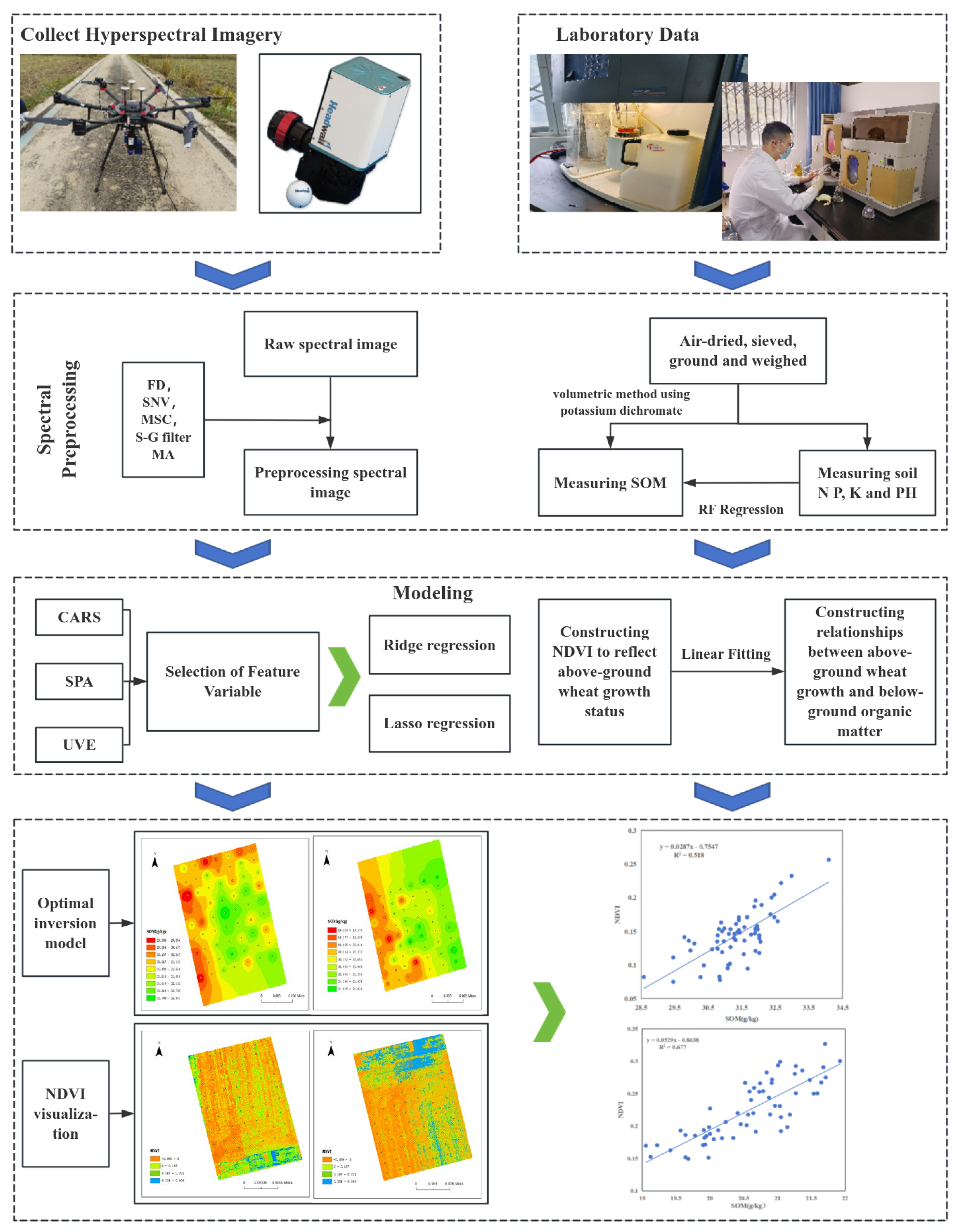
2.1. Research Technology Process

Based on the corrected hyperspectral data (hereinafter referred to as “raw spectral data”), the raw spectral data were subjected to first-order derivative (FD), multiplicative scatter correction (MSC), standard normal variate (SNV), Savitzky–Golay (SG) smoothing, and moving average (MA) smoothing preprocessing operations to suppress the noise in the spectral data. Subsequently, the preprocessed spectral data were downscaled using competitive adaptive reweighted sampling (CARS), successive projections algorithm (SPA), and uninformative variables elimination (UVE) algorithms to extract the characteristic bands. On this basis, ridge regression and Lasso regression models were used to construct the inversion model, compare the inversion accuracy of SOM content of each model, and use the optimal inversion model to visualize and express the organic matter content of the experimental plots, and at the same time, calculate the aboveground NDVI index to reflect the wheat growth situation map, and construct the linear relationship between the underground organic matter content and the aboveground biomass. The whole experimental process is shown in Figure 1.

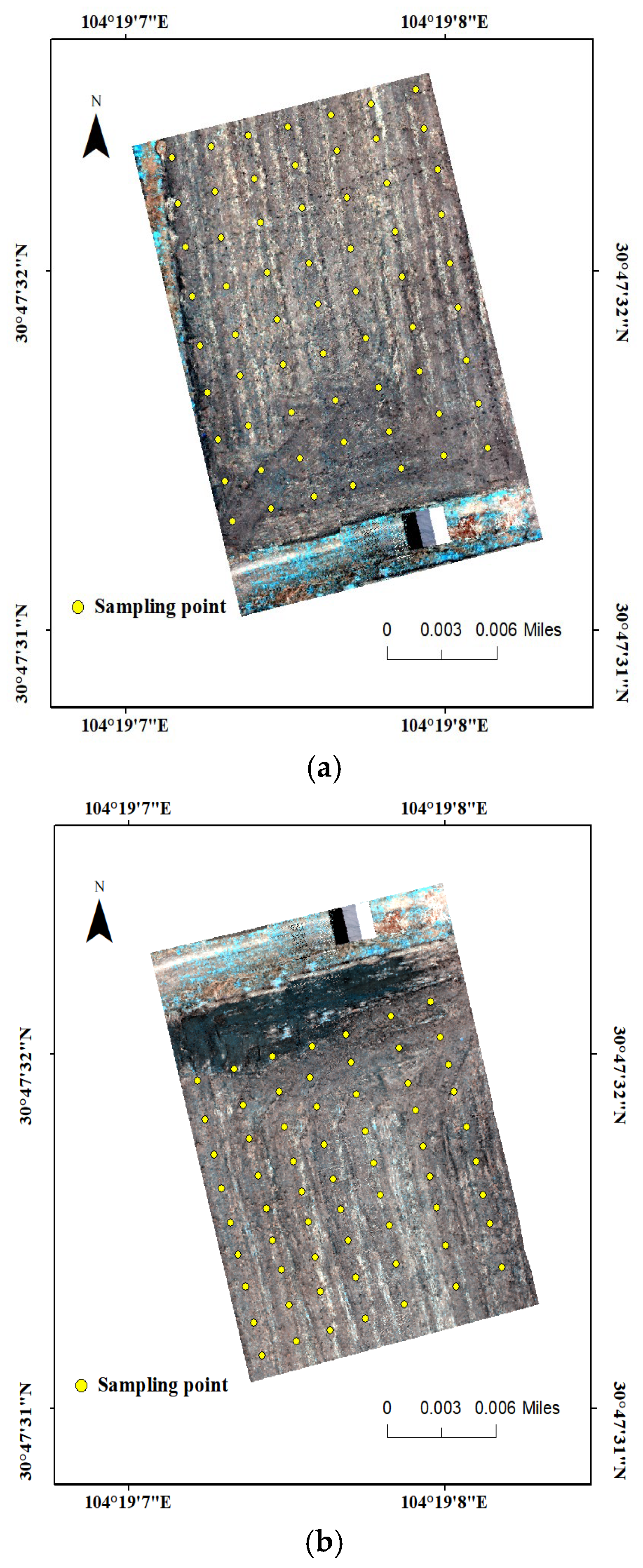
2.2. Study Area and Experimental Design

The experimental site was located in the experimental field of Yao Du Town, Qingbaijiang District, Chengdu City, Sichuan Province, China. Yao Du Town has a subtropical mild and humid climate, characterized by a slight temperature difference between winter and summer, uniform seasonal distribution of precipitation, and climatic conditions suitable for planting crops such as wheat, rice, and corn. The crop grown in the test field is winter wheat, and the planting system of the test field is winter wheat–summer rice rotation. Different fertilization treatments were made in two adjacent experimental fields of about 60 m × 30 m size, where field 1 was manually fertilized with compound fertilizer, which was spread evenly over the whole field and tilled into the soil one week before sowing, and field 2 was not fertilized (the data were only used for subsequent comparative analysis). The effect of fertilizer application on SOM can be visually assessed by comparing the SOM data of the fertilized and unfertilized fields. The topsoil layer is the main SOM enrichment layer, where microbial activities and plant residue decomposition are concentrated, with higher SOM content and significant spatial variability, which is more likely to be captured by hyperspectral sensors. The proportion of exposed soil between wheat rows is high, and compared with the canopy-covered area, soil spectral information can be obtained more directly. Sampling points were set up every 3 m in the experimental field, and small flags were inserted in each soil sampling point in order. About 200 g of topsoil (0–15 cm) was collected from each sampling point and placed in numbered plastic bags, and a total of 126 samples were collected to ensure that the spectral data corresponded to the soil sampling data. The sampling points were evenly distributed throughout the study area, as shown in Figure 2. The blue area in the picture is the weeds. The data from Field 1 were used for inverse modeling, and the data from Field 2 was used for analysis and comparison. All samples were transported to the laboratory for air-drying, grinding, and sieving (particle size ≤ 0.15 mm) after collection, and the organic matter content of the soil samples was detected using the volumetric method of potassium bicarbonate. The maximum, minimum, mean, and variance values are shown in

Table 1. Basic information of soil samples.

	Test Area	Max	Min	Average	Standard Deviation	Coefficient of Variation
SOM (g/kg)	Field 1	34.091	28.580	31.326	0.991	3.161%
	Field 2	21.924	19.053	20.612	2.612	12.869%

.

2.3. Hyperspectral Data Acquisition

The DJI M600 Pro UAV equipped with the Headwall airborne hyperspectral imager (DJI, Shenzhen, China) was used as the experimental flight platform. The imaging spectrometer features a wide range of wavelengths, a spectral resolution of up to 4 nm, wide coverage, and high sensitivity, and can accurately capture the subtle spectral features of surface objects at specific wavelengths. The spectral bands collected in the experiment ranged from 884–2442 nm, with a band interval of 10 nm, and the hyperspectral data were collected in a sunny and cloudless midday period during the wheat sprouting period when the sun’s altitude angle was moderate and the illumination conditions were stable, which was conducive to the acquisition of high-quality hyperspectral data. The shooting height was 30 m and the exposure time was 0.5 s, the flight speed was 7 m/s and the route was set up in an S-shape to cover the whole area of the study area by planning multiple parallel routes. Before each data acquisition, a 3rd order calibration plate was used as a known reflectance object so that the spectral reflectance of other objects could be calculated. After radiometric calibration, atmospheric correction, geometric correction, image stitching, and removal of water vapor absorption bands, a total of 143 valid bands were retained for further analysis.

2.4. Spectral Data Preprocessing

During hyperspectral data acquisition, the raw spectra usually contain irrelevant information due to a variety of factors such as sample surface inhomogeneity, instrumental baseline drift, random noise, and light scattering. To improve the validity of the data and the accuracy of model predictions, we compare five preprocessing methods, including FD, MSC, SNV, SG smoothing, and MA smoothing. The FD method highlights subtle variations in the data by removing baseline drift and background noise and aims to highlight absorbance features contained in the spectra, eliminating additive and multiplicative effects on the spectra [37]. The SNV conversion standardizes the data by removing bias between different measured variables, thus improving data consistency and reliability [38]. The primary goal of the MSC is to reduce or eliminate the influence of the physical characteristics of the sample on the spectral data [39]. SG smoothing is an optimal segmentation fitting method based on polynomials in the time domain using least squares by moving the window and is widely used for data stream smoothing and denoising [40]. MA smoothing algorithm smooths the data by calculating the average of each data point with its several surrounding data points to remove noise [41].

2.5. Extraction of Characteristic Bands

The main objective of feature extraction is to reduce the data dimensionality and eliminate irrelevant or incorrect information that may affect the final classification result. Due to the high dimensionality of hyperspectral data, feature selection is performed before modeling. Feature selection techniques are utilized to identify a subset of metrics with the least covariance, negligible redundancy, and valuable information to effectively represent hyperspectral data.

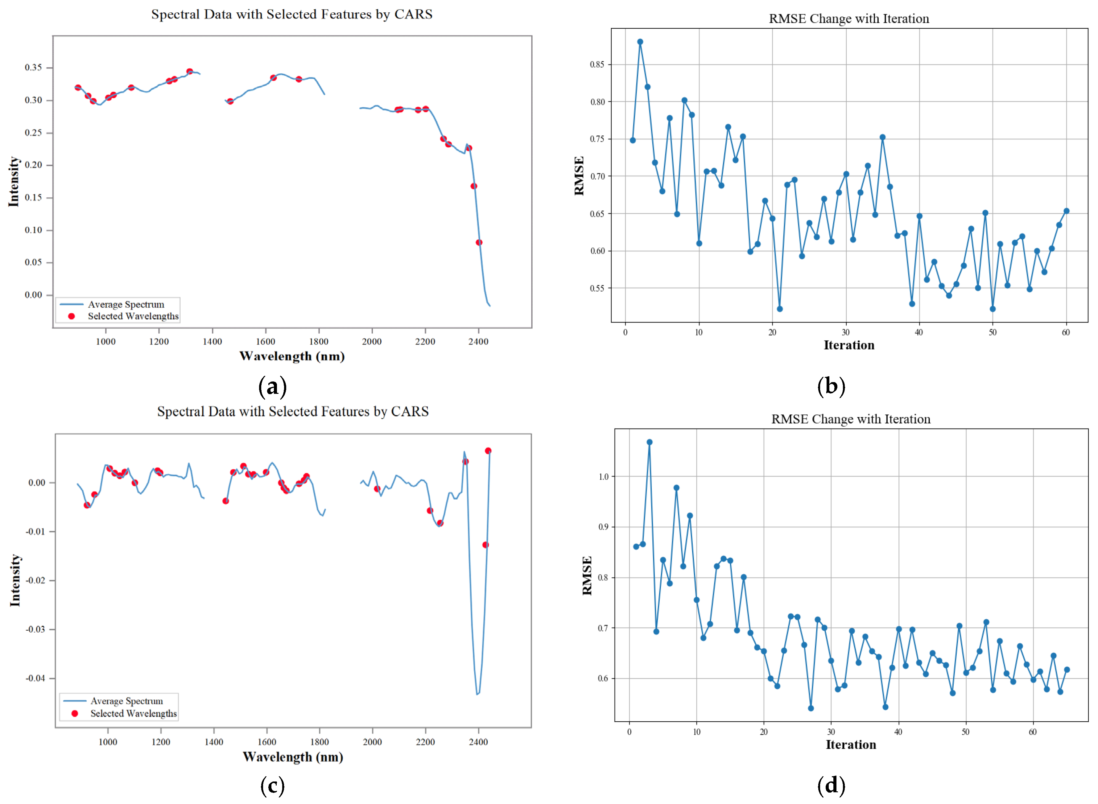
2.5.1. Competitive Adaptive Reweighted Sampling Algorithm

CARS is a feature variable selection method for processing high-dimensional spectral data, which combines Monte Carlo sampling with the regression coefficients of a PLS model, and continuously adjusts and optimizes the selection of wavelengths through an iterative process to retain the wavelengths with the greatest contribution to the model prediction [42]. In CARS, adaptive reweighted sampling is used each time, and the points with larger absolute weights of regression coefficients in the PLS are retained as a new subset, and the points with smaller weights are removed. Then, a PLS is built based on the new subset. After performing several calculations, the subset of wavelengths with the smallest cross-validated root-mean-square error is selected as the characteristic wavelength using the PLS [43].

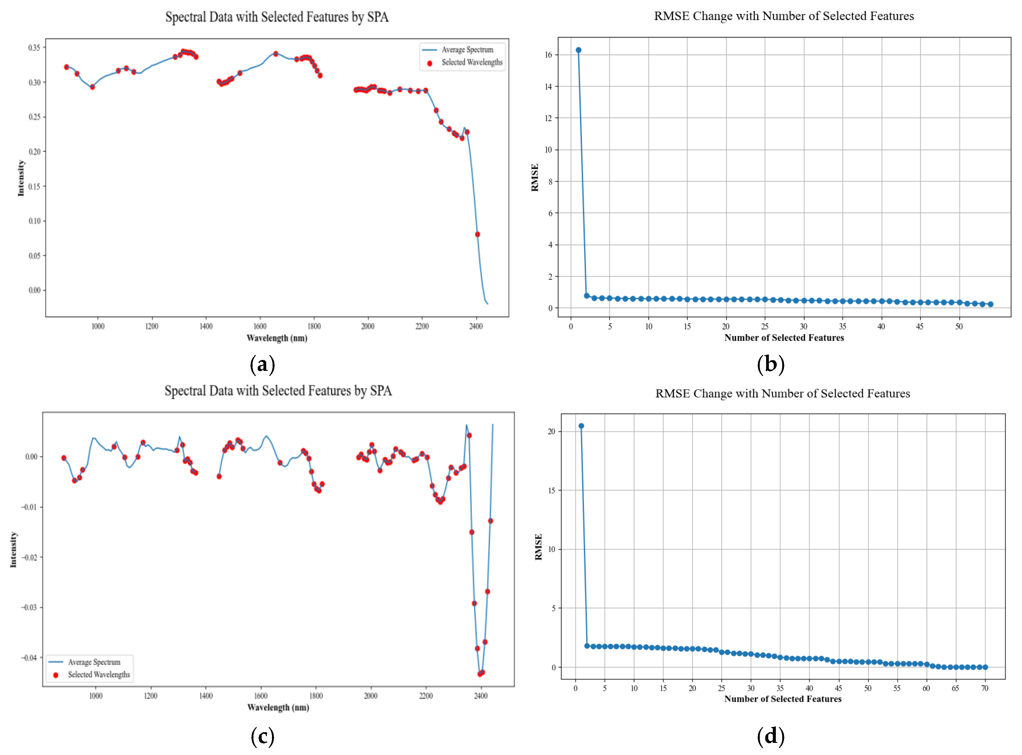
2.5.2. Successive Projections Algorithm

The SPA algorithm is a forward selection algorithm designed to select the wavelength with the least redundancy [44]. It reduces redundant information and improves model performance and interpretability by progressively selecting the most relevant features. The algorithm calculates the projections of randomly selected wavelengths to other wavelengths selects the wavelength with the largest projection vector as the candidate wavelength, and calculates the RMSEP value when selecting the optimal wavelengths, where the subset corresponding to the minimum value is the optimal subset of the wavelengths [45,46]. The SPA is highly noise- and variability-resistant and can stably identify the features that contribute most to the model and can effectively eliminate covariance and redundant information in the spectrum [47,48].

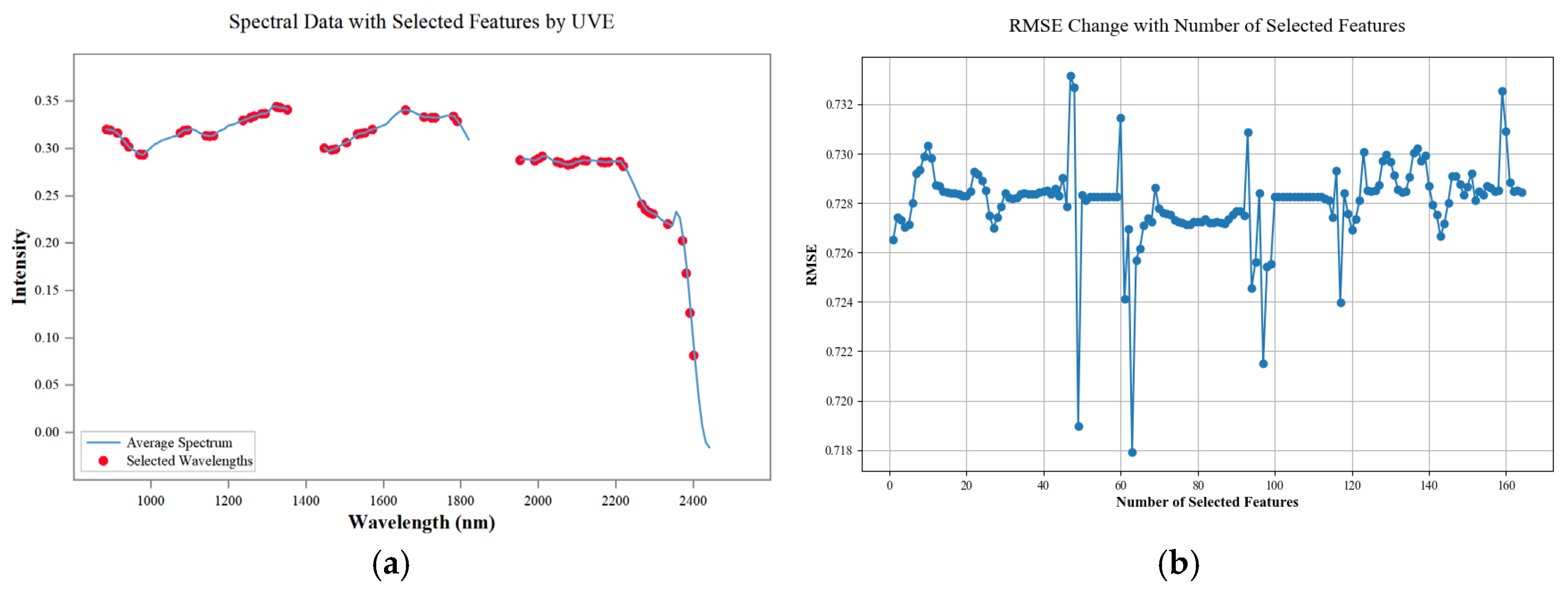
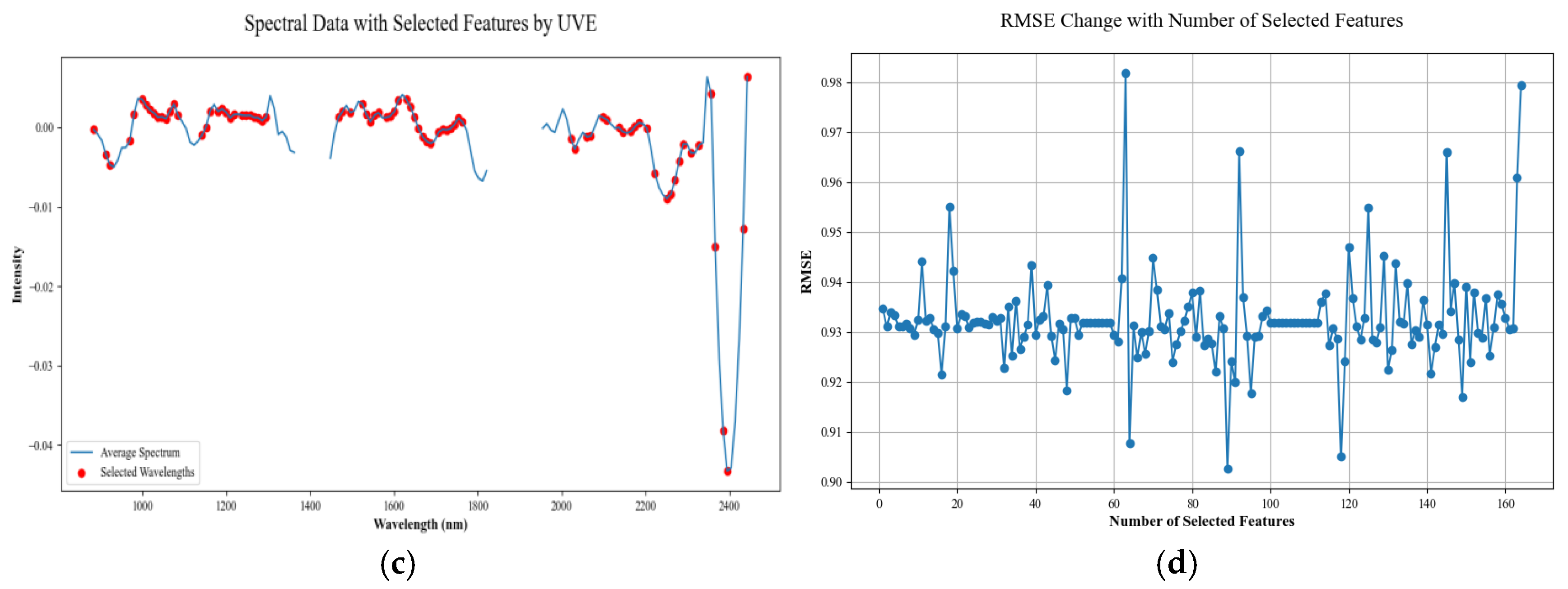
2.5.3. Uninformative Variables Elimination Algorithms

UVE is an algorithm based on the stability of regression coefficients in PLS regression that eliminates uninformative variables and efficiently selects useful wavelength variables [49]. UVE has a significant advantage in selecting wavelengths because it combines noise and spectral information to extract the characteristic wavelengths of the spectra, and the results of the selection process are easier to interpret. This method ensures that only useful wavelengths are retained for further analysis [50].

2.6. Model Construction and Evaluation

2.6.1. Ridge Regression Model

Ridge is an extension of linear regression that introduces regularization to address the problem of multicollinearity that can occur in ordinary least squares [51]. Multicollinearity is a situation where features are highly correlated, which can lead to model instability and overfitting. In addition, with small sample data, regularization can help the model generalize better to unseen data. The objective function of Ridge is:

$$\mathrm{J}\left(\mathrm{\beta }\right)=\parallel \mathrm{y}-\mathrm{X}\mathrm{\beta }{\parallel }_2^2+\mathrm{\alpha }\parallel \mathrm{\beta }{\parallel }_2^2$$

(1)

where $\mathrm{J}\left(\mathrm{\beta }\right)$ is the objective function, y is a vector of objective values, and X is the identity matrix, β is a vector of model parameters, and α is a hyperparameter that controls the strength of the regularization. A balance between minimizing the sum of squared residuals and the regularization term is achieved by adjusting α: when α = 0, Ridge is equivalent to ordinary least squares; if α increases, the effect of the regularization term is enhanced, thus limiting the growth of the model parameters and mitigating the effects of multicollinearity [52].

2.6.2. Lasso Regression Model

The Lasso algorithm was proposed by Robert Tibshirani in 1996 for parameter estimation and variable selection in regression analysis [53]. Designed to solve the problem of fitting a model with a large number of variables and a small sample size, Lasso adds an L1 norm penalty term to the least squares method to compress the estimated parameters. In contrast to ridge regression, which minimizes the sum of squared errors, Lasso regression attempts to balance model complexity and predictive accuracy by penalizing the absolute value of its coefficients [54]. By converting each coefficient to a constant component and truncating at zero, Lasso regression minimizes the residual sum of squares while constraining the sum of absolute values of the coefficients. The objective function for Lasso regression is

$${\mathrm{ARGMIn}}_{\mathrm{\beta }}\left\{ | \mathrm{r}-{\sum }_{\mathrm{i}=1}^{\mathrm{N}}\mathrm{X}\mathrm{j}\mathrm{\beta } {|}^2+\mathrm{\lambda }{\sum }_{\mathrm{i}=1}^{\mathrm{N}}|\mathrm{\beta }|\right\}$$

(2)

where Y is the response variable, X_j is the predictor variable, and β is the coefficient variable. λ is the regularization parameter that controls the strength of the coefficient penalty. By manually setting the possible range of λ values, cross-validation is used for each λ value to evaluate the model performance, thus selecting the value of λ that optimizes the model performance [55].

2.6.3. Model Evaluation

In this study, the reliability and accuracy of the model inversion are judged by the determination coefficient (R²) and the root mean square error (RMSE) of the validation set. R² reflects the degree of fit of the model to the data, and the closer the R² is to 1 indicates that the estimated model is more interpretable to the data. RMSE reflects the accuracy of the model, with lower RMSE indicating higher accuracy of the estimated model. The model was randomly divided into training and test sets in the ratio of 7:3, and the constructed model was used to predict the soil nitrogen content.

Statistical testing is determined by statistical theory and is aimed at testing the statistical properties of the model. It is the use of mathematical statistics to test the equations and the reliability of the estimates of the model parameters. We calculate the value of the statistic F to show whether the overall linear relationship between the explained variables and all explanatory variables is significant.

3. Results and Discussion

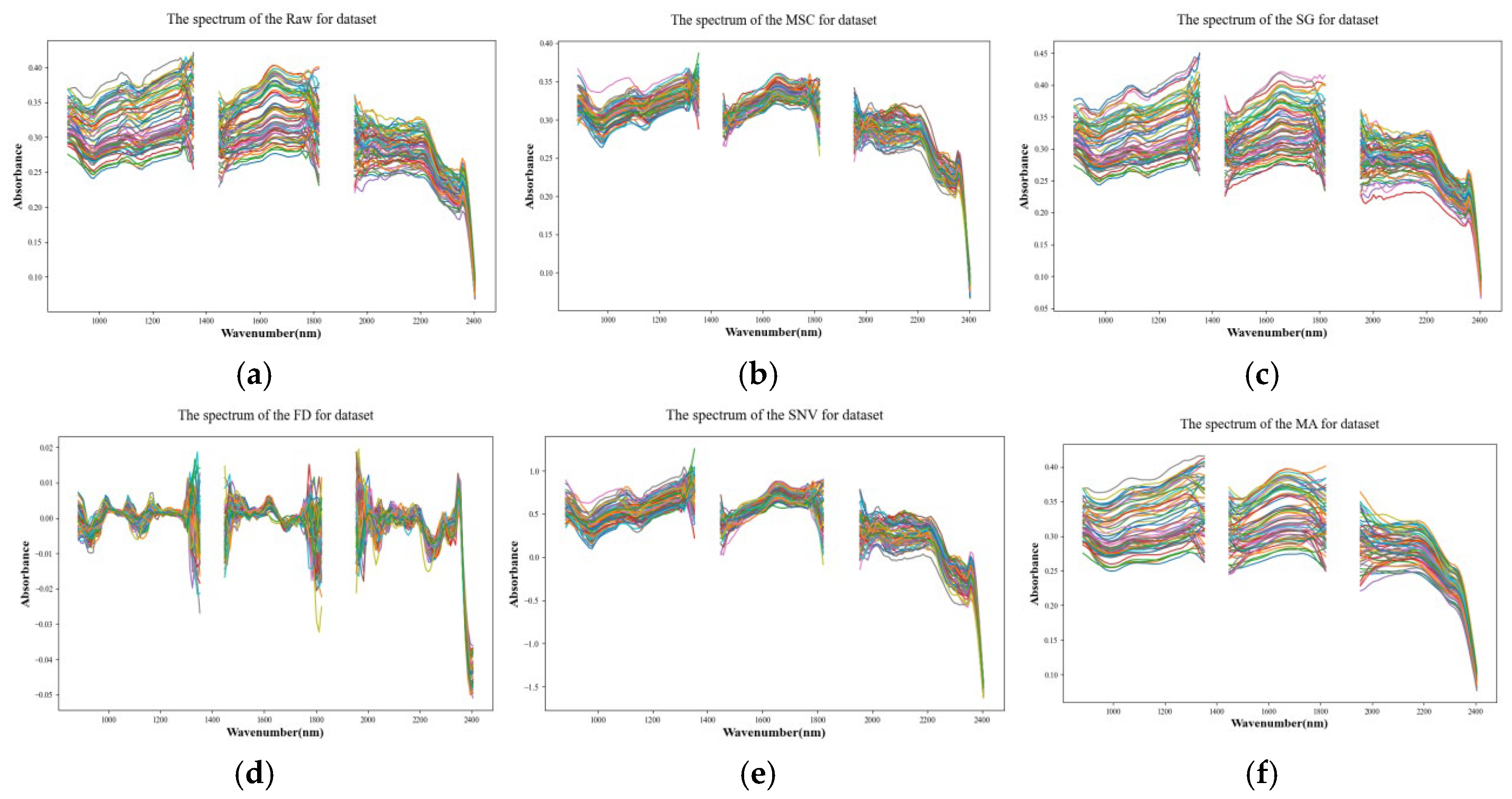
3.1. Effect of Spectral Pre-Processing

Figure 3 shows the raw spectral curves of the soil samples from Field 1 and their mathematical transformations. Each curve in Figure 3 represents a soil sample data. From Figure 3a, it can be seen that there are obvious differences in the raw reflectance between the samples and there are phenomena such as baseline shift and tilt between the spectra. After MSC and SNV treatments, the differences in reflectance were significantly reduced, and the spectra showed higher concentration and consistent spectral curve characteristics. It is demonstrated that these two spectral transformation methods can effectively resolve spectral offsets, eliminate background interference and noise, and enhance spectral features. The FD transformation effectively highlights small variations in the spectra, including the locations of reflectance peaks and valleys, which reduces background interference and improves the accuracy of feature extraction. After preprocessing with the SG smoothing and MA algorithms, the feature information of the original spectra is retained and the noise interference is reduced, providing a more accurate and stable basis for subsequent spectral analysis.

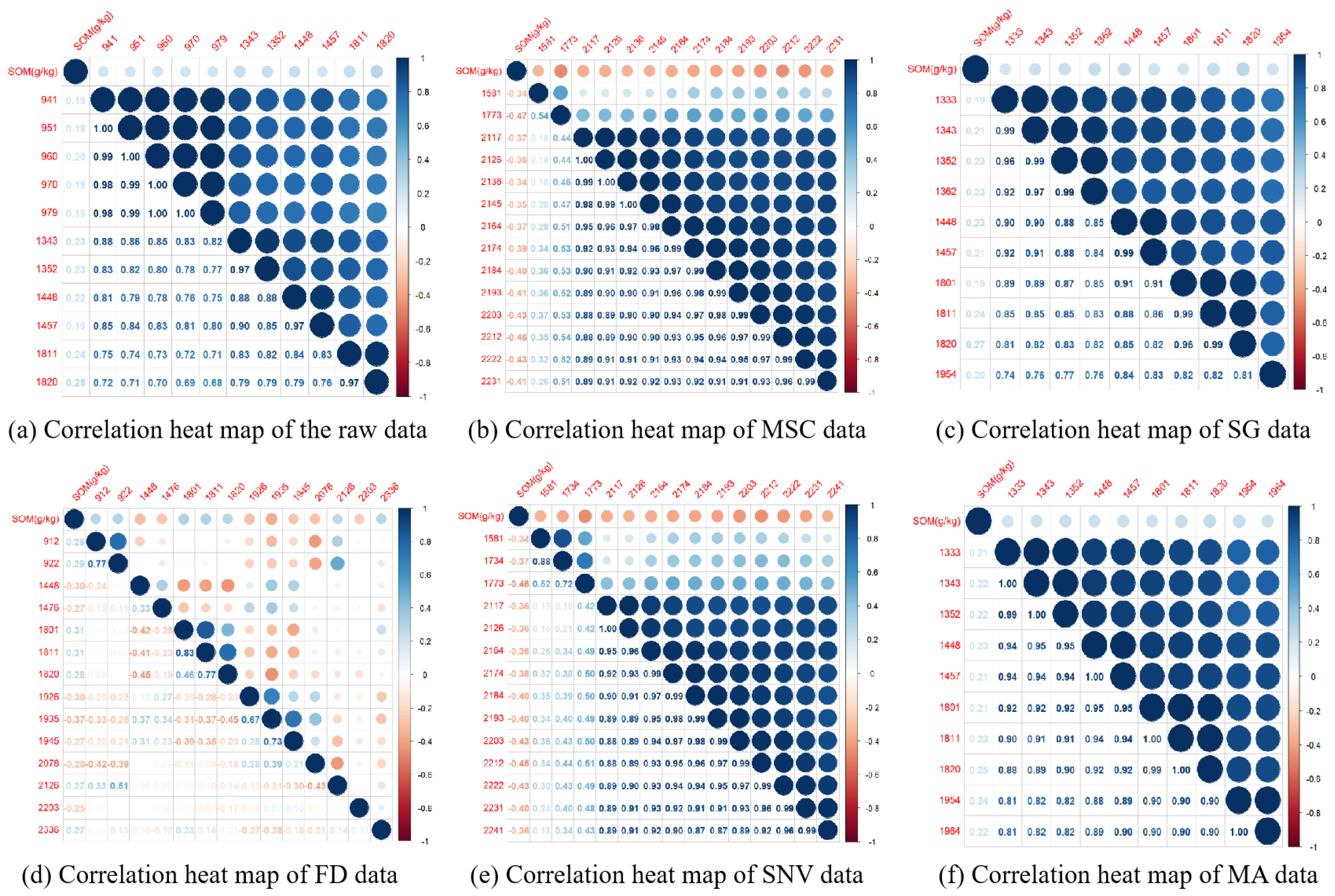
3.2. Correlation Analysis

Figure 4a–f shows the Spearman’s correlations between the raw spectral data and the five preprocessed data with the measured values of soil SOM. From Figure 4a, it can be seen that the correlation between the raw spectral data and the measured values of soil SOM is weak, with no significant correlation coefficient, and there is a problem of multiple covariance between the bands. The correlation coefficients between the spectral data and soil SOM content were significantly higher after MSC and SNV pretreatment. The maximum correlation coefficient between the spectral reflectance and the measured value of SOM after SNV treatment was −0.463 (e.g., Figure 4e), and the maximum correlation between the spectral reflectance and the measured value of SOM after MSC treatment was reached (R = −0.472 **) (** indicates p < 0.01) (e.g., Figure 4b). The correlation coefficients between spectral data and soil SOM content were significantly improved after FD preprocessing, while the problem of covariance between spectral data was weakened (e.g., Figure 4d). The SG and MA preprocessing were less effective in improving the correlation between the spectral data and SOM content and did not reduce the covariance interference between the spectral data, (e.g., Figure 4c,f). Based on the analysis of the results, it can be seen that the two pre-processing of FD and MSC are the most effective. Among them, more significant correlation coefficients were observed in the ranges of 1450–1480 nm, 1581 nm, 1773 nm, and 1800–2330 nm. The band attached to 1400 nm is affected by water vapor absorption peaks and exhibits higher correlations. The C-H bonds in organic matter can be detected at wavelengths around 1700 nm [56] Vibrations of the N-H and C-O structures show spectral features at about 2100 nm, which are considered to be closely related to SOM. Our results are in agreement with previous findings reported in the literature [16,57]. The spectral band around 2200 nm is associated with Al-OH groups in clay minerals and is an important indicator of organic matter [58,59]. Ben-Dor et al. [60] found that the spectral band around 2300 nm was associated with aromatic ring or aliphatic carboxyl group linkages of organic matter in soil. The numerous characteristic bands of SOM in the near-infrared spectral range help to fit the relationship between spectral data and SOM content in SOM inversion models.

3.3. Feature Band Extraction Analysis

Although preprocessing can successfully reduce the impact of noise and scattering on spectral data analysis, redundant and overlapping band data still exist in full−spectrum data [61]. The use of full-band modeling not only leads to computational inefficiency but also reduces the prediction accuracy of the model [62]. Therefore, for preprocessed full−spectrum data, wavelength filtering is required to minimize the data dimensionality and remove information that is not necessary for detection indication. This speeds up model training and improves prediction accuracy [63]. In this study, feature band extraction was performed based on MSC and FD preprocessed spectral data. The importance of features or subsets of features is measured based on the RMSE values, i.e., to quantify the connection between feature variables and target variables as well as the interconnections between features. To avoid overfitting, cross-validation was used to assess the goodness of features and to test the validity of the selected modeling set in the validation dataset, with the number of cross-validation pairs being 10.

Figure 5a,c depict the corresponding positions of the filtered feature wavelengths of the CARS algorithm in the spectrum, and Figure 5b,d show graphs of its RMSE value with the number of iterations. When the CARS algorithm is based on MSC preprocessed data for feature extraction, the minimum RMSE value is 0.522, and its corresponding iteration number is 25, corresponding to the number of selected variables is 21. The feature bands are more densely distributed in the ranges of 890−1280 nm and 2100−2400 nm, and more sparsely distributed in the range of 1460−2090 nm; When the CARS algorithm performs feature extraction based on FD preprocessing data, the minimum RMSE is 0.524, and its corresponding iteration number is 52, corresponding to the number of selected variables is 27. The feature bands are densely distributed in the ranges of 890−1200 nm and 1448−1753 nm, and sparsely distributed in the range of 1763−2442 nm. The CARS algorithm tends to select fewer but representative feature bands, and its screened feature bands are more uniformly distributed throughout the spectral curve. However, due to the small number of feature bands extracted, there may be a certain loss of information.

Figure 6a,c depict the corresponding positions of the feature wavelengths extracted by the SPA algorithm in the spectrum, and Figure 6b,d show graphs of its RMSE value with the number of extracted feature bands. When the SPA algorithm is based on the MSC preprocessing data for feature extraction, the minimum RMSE value is 0.35, and the corresponding number of selected variables is 54; When the SPA algorithm is based on the FD preprocessing data for feature extraction, the minimum RMSE is 0.05, and the corresponding number of selected variables is 64. The feature bands extracted by the SPA algorithm are mostly distributed at the inflection points of the spectral curves, and the distribution is more dispersed within the whole spectral curve. The number of feature bands extracted based on the FD is higher and more evenly distributed, because the SPA algorithm can efficiently and accurately extract more feature variables when the feature bands in the spectral data are clearer.

Figure 7a,c depict the corresponding positions of the feature wavelengths extracted by the UVE algorithm in the spectrum, and Figure 7b,d show graphs of the variation of its RMSE values with the number of extracted feature bands. When the UVE algorithm is based on MSC preprocessed data for feature extraction, the minimum RMSE value is 0.7178, and its corresponding number of selected variables is 63; when the UVE algorithm is based on FD preprocessed data for feature extraction, the minimum RMSE is 0.903, and its corresponding number of selected variables is 89. Its extracted feature bands are not only mostly distributed at the inflection points of the spectral curve, but also densely and uniformly distributed within the whole spectral curve, and it extracts the largest number of feature bands. This helps to capture the subtle changes in the spectral data and improve the sensitivity and accuracy of the subsequent modeling. Due to the high number of extracted feature bands, the UVE algorithm requires additional computational resources and time to process these data.

3.4. Regression Model Analysis

To investigate the influence of SOM content on the growth and development of winter wheat, the spectral data of the characterization variables obtained from six different fusion strategies (MSC-CARS, MSC-SPA, MSC-UVE, FD-CARS, FD-SPA, and FD-UVE) were used as the input factors, and the SOM content was used as the output factor, and the ridge regression-based and Lasso based ridge regression and Lasso estimation models of SOM content, respectively. The predictive ability and accuracy of the models were evaluated by fitting the predicted and measured values to the measured data.

Figure 8 and Figure 9 show the modeling accuracy of each feature extraction algorithm after MSC and FD preprocessing, respectively. From the figures, we can infer that CARS shows the lowest performance. When there are a large number of redundant bands in the spectral data, although CARS can effectively reduce the spectral dimensions and reduce the complexity of the model, its extracted features cannot fully explain the spectral properties of SOM, so its extracted features have limitations in improving the modeling accuracy. The SPA algorithm shows good performance, indicating that the SPA algorithm is suitable for processing high-dimensional spectral data, and can effectively screen out the feature bands that have higher explanatory ability for the SOM. The UVE algorithm is suitable for processing high-dimensional data containing a lot of noise and redundant information and has wide applicability. Therefore, when there is a complex relationship between SOM and spectral data, the UVE algorithm is more advantageous and effectively improves the accuracy of the model. As can be seen from the figure, the model that obtained the optimal results based on Ridge regression was FD-UVE-Ridge (Figure 8f) (R² = 0.889, RMSE = 0.325), F = 2.44 (p < 0.05), and the model that obtained the optimal results based on Lasso regression was FD-UVE-Lasso (Figure 9f) (R² = 0.961, RMSE = 0.180), F = 8.78 (p < 0.05). The Lasso regression model is generally more accurate than the ridge regression model for the same number of characteristic variables. This is due to the sparsity property of Lasso regression, which makes it more capable of filtering out the feature variables that are important for the estimation of SOM content, thus reducing the effect of noise and redundant information. As the number of feature variables increases, the accuracy of both regression models improves, but the improvement in the accuracy of the Lasso regression model is greater, which further validates the advantages of Lasso regression in feature selection and model optimization.

3.5. Analysis of the Relationship Between Below-Ground Organic Matter and Above-Ground Crop Growth

The model performance varies depending on the modeling algorithm and spectral transformation, we chose the best-performing model among the above models and substituted the fitting equations into the spectral images to produce the inverse distribution maps of organic matter content in the 2 experimental fields. Using the inverse distance weighting method, we spatially interpolated the SOM content and generated a visualization map of SOM content for a more intuitive view of the SOM distribution pattern, as shown in Figure 10. Figure 10a shows the field with fertilizer application, and from the inversion results, it can be seen that the organic matter content ranges from 28.624–33.325 g/kg, and the inversion results are within the range of the measured values, which basically overlap with the range of the measured values. The distribution of organic matter content in the whole field is relatively uniform and moderate, which is suitable for the growth and development of wheat seedlings. Figure 10b shows a field without fertilization, with organic matter content ranging from 19.337–21.575 g/kg, which is basically consistent with the range of measured values, but the overall organic matter content is on the low side and is not conducive to the subsequent development of wheat seedlings. After the above analysis, we used the inversion results of the optimal model to calculate the normalized difference vegetation index values (NDVI) of the spectral images of different fields to visualize the crop growth, as shown in Figure 11. Specifically, field 1 showed superior crop growth, in which the growth rate of wheat was relatively uniform and consistent, which was conducive to improving the overall yield and quality of the crop. There was a small amount of weed cover in the field canopies and field edges, which is shown in blue in the figure. Field 2 showed unstable growth, as can be seen from the figure, with weed cover in the field canopies, field edges, and the middle of the field, and sparse growth of the wheat seedlings. This indicates that the nutrients in the soil were insufficient and too many nutrients were sucked up by the weeds, resulting in some of the seedlings not growing properly. The experimental results showed that the organic matter content of the fertilized field was significantly higher than that of the unfertilized field, and the wheat in the fertilized field grew better, showing higher aboveground biomass and healthier plant morphology, which verified the positive correlation between the aboveground biomass and the belowground organic matter content.

Subsequently, we matched the NDVI values and the measured SOM data of the two field sampling sites one by one and used linear regression analysis to reveal the potential relationship between the subsurface SOM content and the above-ground crop growth. Figure 12 clearly demonstrates that there is a linear correlation between the two. From the figure, we can see that the R² value of field 1 is 0.518 and that of field 2 is 0.677, both of which have a more obvious linear relationship. In field 1, the unevenness of manual fertilization resulted in a more dispersed distribution of the measured values of SOM, and thus the accuracy of the regression model was affected. However, after the fertilization operation, we can clearly see that the SOM content is higher in field No. 1, and the growth of wheat on the ground is better. This further verifies that the increase of SOM content can promote the growth of ground crops. In summary, our results not only confirm the existence of a linear relationship between SOM content and crop growth but also emphasize the importance of rational fertilizer application for improving crop yield. This implies that it is crucial to adopt a scientific fertilizer application strategy in agricultural production to maximize the overall crop growth effect.

4. Discussion

4.1. Characteristic Band Analysis

We observed more significant correlation coefficients with SOM content in the 1450–1480 nm, 1581 nm, 1773 nm, and 1800–2330 nm band ranges, which is in agreement with previous studies [15,64,65,66]. These sensitive bands are important for predicting SOM content. This study analyzes the effects of these three algorithms in extracting feature variables in terms of the number of feature bands, the distribution of feature bands, and the accuracy of the model. Some of the feature bands extracted by the CARS algorithm overlap with the sensitive bands of the SOM. The CARS algorithm filters the optimal band combinations by adaptively adjusting the selection probability, and when there are a large number of redundant bands in the spectral data, it can adaptively eliminate the unimportant bands, gradually screen the feature bands through an iterative process, and select fewer but representative feature bands. This streamlined combination of feature bands helps to reduce the complexity of the model but may lose some of the useful information, resulting in limited model accuracy. The SPA algorithm focuses more on extracting the feature wavelengths with the largest variations (i.e., peaks or valleys), and when the feature bands in the spectral data are more explicit, the SPA algorithm is more efficient and accurate, and it is capable of extracting more feature variables while maintaining a higher level of model accuracy. Both SPA and CARS algorithms focus on screening the optimal combination of wavebands from spectral data, while the UVE algorithm focuses more on wavelength screening based on the stability of the PLS regression coefficients. This implies that the UVE algorithm may focus more on the correlation between the bands and the measured values of organic matter when screening the bands. The UVE algorithm extracted the largest number of characteristic bands, which were densely and uniformly distributed and overlapped the most with the sensitive bands of the SOM. This indicates that the UVE algorithm can comprehensively capture spectral information and is suitable for processing complex spectral data with higher modeling accuracy. Therefore, the UVE algorithm is more advantageous for the complex relationship between SOM and spectral data in this study. However, it should be noted that the computational complexity of the UVE algorithm may be relatively high because it needs to perform multiple PLS regressions to calculate the stability and significance of the regression coefficients.

4.2. Model Selection and Evaluation

In the field of machine learning, seeking a solution is essentially the process of continuously searching for learning models with strong generalization ability and high robustness in the hypothesis space [67]. This process suffers from strong sensitivity to training samples, high computational complexity, and overfitting [68]. Li et al. [3] combined image and spectral features of a two-branch convolutional neural network to predict soil organic matter content and obtained good results. However, regression prediction for small sample datasets usually chooses simple linear models such as support vector machines and PLS models to avoid overfitting. The inversion accuracy of the model needs to be considered in addition to overfitting, and other factors such as the multicollinearity problem between independent variables [69]. Ridge regression and Lasso regression models have significant advantages in dealing with these problems. Ridge regression can solve the multicollinearity problem effectively by adding the sum of squares of regression coefficients as a regularization term in the loss function. Ridge regression can provide stable estimates of regression coefficients when there is a high degree of correlation between the independent variables. In addition, ridge regression reduces the complexity of the model by introducing a regularization term, which reduces the risk of overfitting, which is especially important for small-sample datasets. Lasso regression can reduce certain regression coefficients to zero, which automatically selects important features and simplifies the model structure. In addition, Lasso regression is particularly suitable for sparse datasets, that is, datasets where most of the eigenvalues are zero or close to zero. This is a big advantage for the spectral reflectance that partially tends to zero in this study. In this case, Lasso regression is more effective in identifying features that have a significant effect on the target variable. Several studies have shown that the Lasso model performs well in predicting crop growth, biomass, and nitrogen accumulation status based on remotely sensed data [70,71], which is consistent with the results of this study. Similar to ridge regression, Lasso regression also prevents the model from overfitting on the training data by introducing a regularization term. The construction of an optimal estimation model using a suitable algorithm in this study can help to accurately estimate the SOM content in the soil. In addition, the study should carry out more research involving different planting crops and different soil properties to collect more representative soil hyperspectral data to further improve the estimation accuracy and applicability of the SOM model.

4.3. Analysis of the Impact of Other Factors

We measured NPK and PH data for soils collected during the same period. Based on two fields with different fertilization conditions, we used the Random Forest algorithm to build a model to quantify the degree of explanation of soil physical properties in terms of NPK content and PH value on SOM to reveal the effect of soil chemical properties on organic matter content. As shown in Figure 13, among them, N content had a significant effect on SOM, with an explanation rate of 50.7% and 62.4%, respectively, mainly because chemical N fertilizer inputs accelerated the mineralization and decomposition of organic matter, and the microbial activity was enhanced, accelerating the decomposition of SOM. It indicates that N is a key factor limiting soil fertility and needs to be supplemented as a priority in subsequent fertilization. The effects of both P and K content and pH on SOM content in fertilized fields ranged from 10–20%; the effects on SOM content in unfertilized fields spanned a wide range from 9–30%, spanning a wide range. Fertilized fields reduced the natural variability of other elements (P, K) and pH through artificial nutrient supplementation, which stabilized their relative effects. In contrast, under unfertilized conditions, soil nutrients are dependent on natural processes (e.g., mineralization, plant residue decomposition), and their contents are more influenced by local environments such as microbial activity and moisture, leading to significant differences in the explained rates of P, K, and pH. Among them, K content had a greater effect of 26.3% on SOM content in unfertilized fields, K indirectly enhances SOM stability by promoting microbiomass carbon accumulation, a result that suggests that K may be the second most important limiting factor in soils after N and that natural deficits in potassium may exacerbate its role in regulating SOM. P promotes microbial synthesis of extracellular polysaccharides and enhances the binding stability of SOM to mineral particles; and organic acid accumulation promotes SOM solubilization and migration through chelation in the region of stable pH, both of which have some effect on SOM.

The NPK levels in the soil can reflect the extent and rate of SOM decomposition, and high levels of NPK may mean that SOM is being rapidly decomposed and releasing nutrients, which can be beneficial to crop growth [72]. Although SOM itself has an important role in crop growth, the amount of NPK in the soil also affects the direct effect of organic matter on the crop. If the soil does not have enough N, the crop may be limited in growth due to lack of nitrogen, even if the SOM content is high. Together, the NPK content of the soil and the SOM content form the basis of soil fertility [73]. By comparing the data from fertilized and unfertilized fields, a more comprehensive understanding of the effects of fertilization on SOM and chemical properties can be obtained, which can help to improve the scientific validity and reliability of the experiment. Based on the modeling results in the experiment, it can be seen that nitrogen is the largest limiting factor for soil nutrients, and potassium is the second largest limiting factor after nitrogen. Therefore, we can formulate a targeted fertilization program, and adjust the fertilizer strategy according to the dynamic changes of soil nutrients to improve the soil structure during the subsequent crop growth process. When analyzing the relationship between organic matter content and crop growth, the comprehensive impact of these factors on soil fertility is taken into account. By quantifying the impact of nitrogen, phosphorus and potassium content and pH on organic matter content, we can accurately identify the limiting factors of soil nutrients, avoid over-fertilizing or nutrient imbalance, and improve the efficiency of fertilizer utilization, which provides a scientific basis and technical support for precision agriculture and promotes the intelligence and refinement of agricultural production.

4.4. Interactions Between Soil and Crops

NDVI is an important indicator to reflect the vegetation cover and growth condition. It is a commonly used remote sensing method to indirectly reflect the growth condition of wheat by calculating the NDVI value on the ground in the study area. The content of SOM was then expressed using the predicted value of the inverse performance of the optimal model. The results of the study showed a positive correlation between SOM content and crop growth on the ground, which is consistent with earlier findings [74]. This positive correlation may stem from the positive effects of SOM on nutrient availability, soil structure, and water retention capacity. There are multiple feedbacks (two-way interactions) between SOM and crops, with SOM influencing crop growth, and crop growth also influencing SOM content through stubble return and root secretions. In this study, we focused on the effects of SOM on crop growth, but this does not preclude the potential effects of crop growth or biomass on SOM. SOM contains nutrients that can positively affect soil water-holding capacity, which in turn affects crop biomass. To sort out the causality of feedback between soil and plant and to assess the dominant direction of causality, each variable in this interaction must have a sufficient degree of independence among its predictors [75], and this is achieved through long-term monitoring and multivariate analyses. Future research should integrate the bidirectional interactions of crop biomass, other soil nutrients, and the soil-crop system to fully reveal the relationship between SOM and crop growth. SOM and the nutrients (especially nitrogen) in it may also affect crop growth. Bidirectional, positive interactions between SOM and crop growth have developed over decades to centuries [76,77], and by investigating the relationship between SOM content and crop growth, we can reveal the mechanism by which soil nutrient supply capacity affects crop growth, and provide a precision fertilizer application and a sustainable development of agriculture with a scientific basis.

5. Conclusions

(1)

The use of spectral data preprocessing methods can reduce data noise, improve the correlation between spectral data and SOM content, and reduce the multicollinearity between spectral data. The three feature extraction algorithms, CARS, SPA, and UVE, each have their own advantages, and for the problem of the existence of redundant features in the hyperspectral data in this paper, the UVE algorithm has the best extraction effect.

(2)

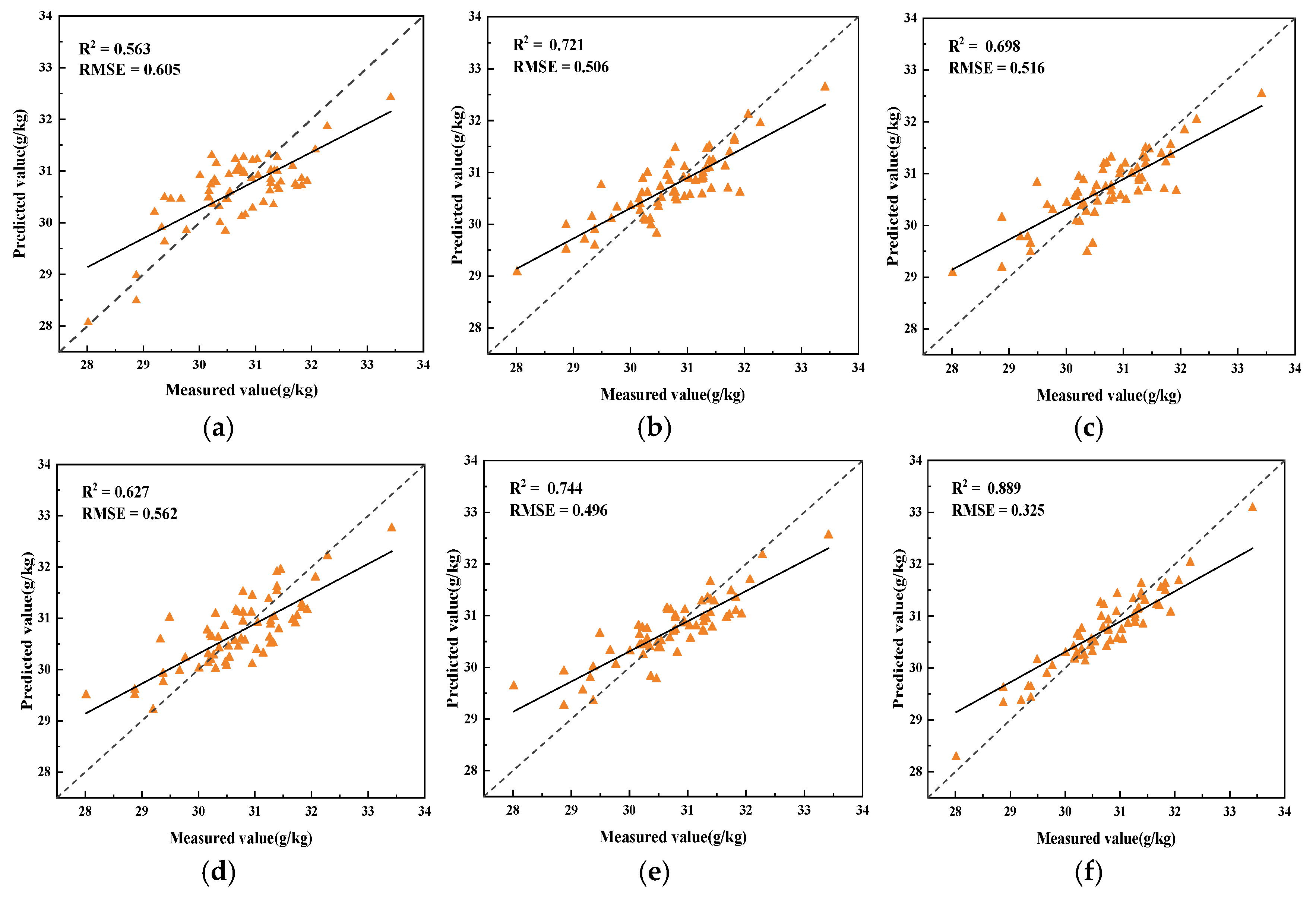
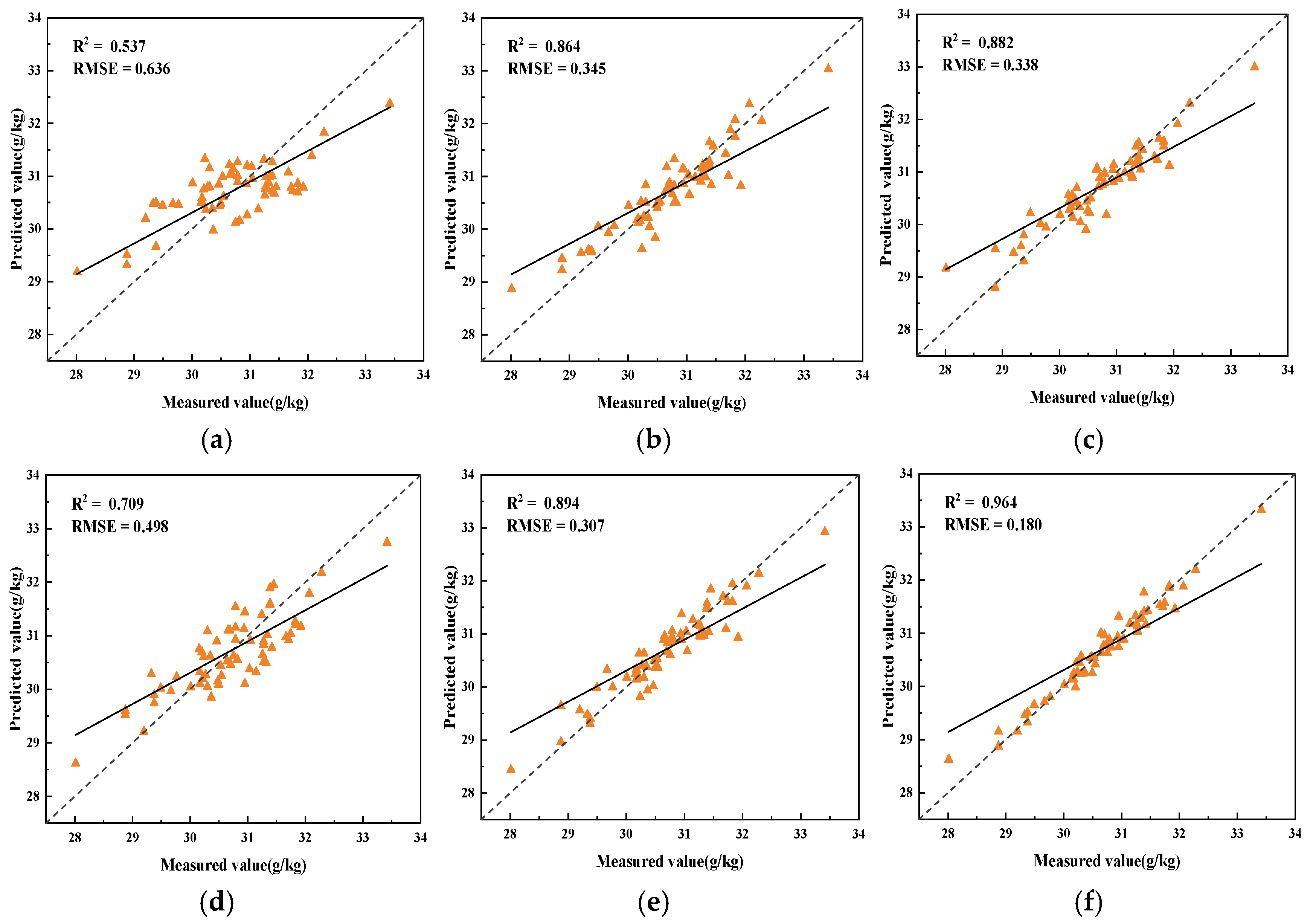
Ridge regression and Lasso regression models have significant advantages in dealing with the multicollinearity problem of hyperspectral data, the model that obtains the optimal results based on ridge regression is FD-UVE-Ridge (R² = 0.889, RMSE = 0.325), and the model that obtains the optimal results based on Lasso regression is FD-UVE-Lasso (R² = 0.961, RMSE = 0.180).

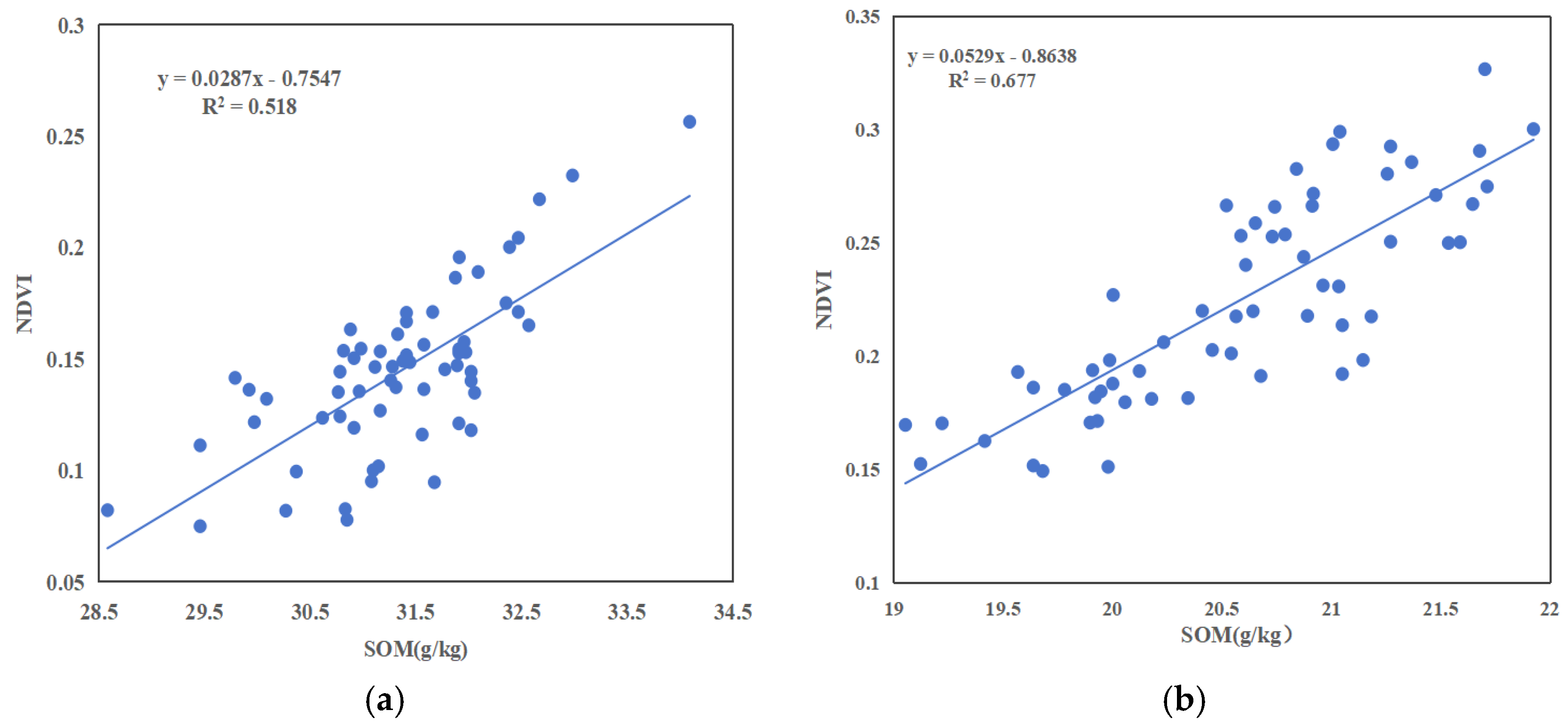
(3)

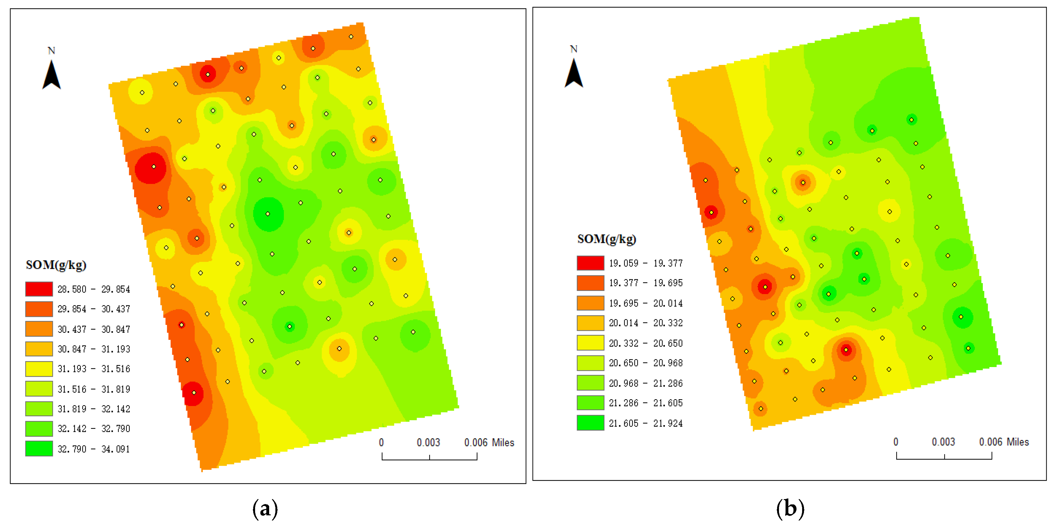
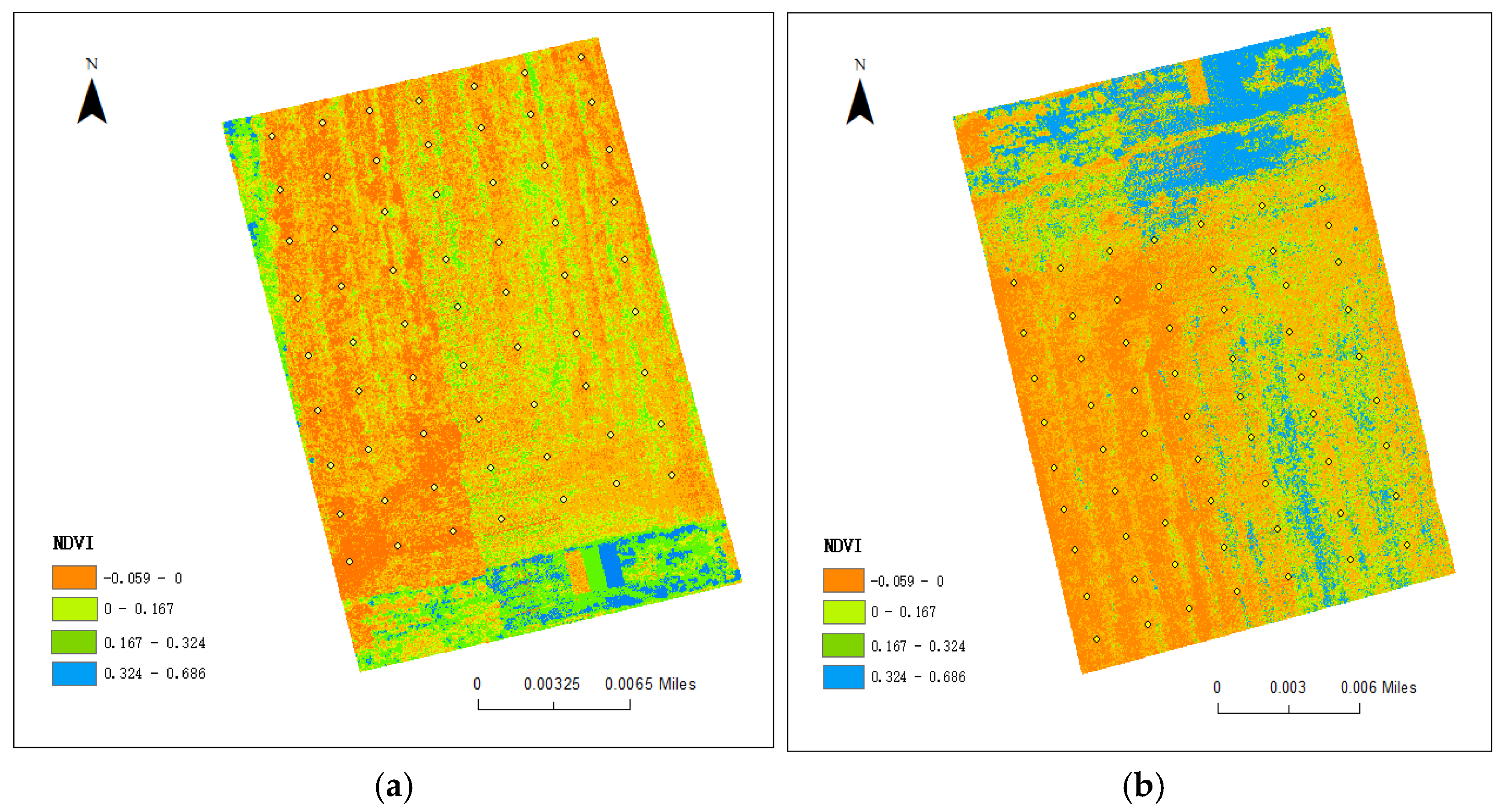
There was a positive correlation between SOM content and above-ground crop growth, in which the accuracy of fitting the above-ground NDVI values to the below-ground SOM content was 0.518 for field 1, and the accuracy of fitting the above-ground NDVI values to the below-ground SOM content was 0.677 for field 2. Fertilizing operations could significantly increase soil SOM content, thus promoting wheat growth.

(4)

The current study lacks continuous observation data from the irrigating stage to the maturity stage of winter wheat, which may weaken the predictive stability of the model in the later stages of the crop growth; in future research, we want to collect In the future, we want to collect the growth data of the whole life cycle of winter wheat to establish an adaptive inversion model with applicability to the whole life cycle.

References

1. Tan, K.; Zhu, L.; Wang, X. A Hyperspectral Feature Selection Method for Soil Organic Matter Estimation Based on an Improved Weighted Marine Predators Algorithm. IEEE Trans. Geosci. Remote Sens. 2024, 63, 5500411. [Google Scholar] [CrossRef]
2. Schmidt, M.W.I.; Torn, M.S.; Abiven, S.; Dittmar, T.; Guggenberger, G.; Janssens, I.A.; Kleber, M.; Kögel-Knabner, I.; Lehmann, J.; Manning, D.A.C.; et al. Persistence of soil organic matter as an ecosystem property. Nature 2011, 478, 49–56. [Google Scholar] [CrossRef] [PubMed]
3. Li, H.; Ju, W.; Song, Y.; Cao, Y.; Yang, W.; Li, M. Soil organic matter content prediction based on two-branch convolutional neural network combining image and spectral features. Comput. Electron. Agric. 2024, 217, 108561. [Google Scholar] [CrossRef]
4. Hong, Y.; Chen, S.; Zhang, Y.; Chen, Y.; Yu, L.; Liu, Y.; Liu, Y.; Cheng, H.; Liu, Y. Rapid identification of soil organic matter level via visible and near-infrared spectroscopy: Effects of two-dimensional correlation coefficient and extreme learning machine. Sci. Total Environ. 2018, 644, 1232–1243. [Google Scholar] [CrossRef]
5. Wan, S.; Hou, J.; Zhao, J.; Clarke, N.; Kempenaar, C.; Chen, X. Predicting Soil Organic Matter, Available Nitrogen, Available Phosphorus and Available Potassium in a Black Soil Using a Nearby Hyperspectral Sensor System. Sensors 2024, 24, 2784. [Google Scholar] [CrossRef]
6. Zhou, T.; Jia, C.; Zhang, K.; Yang, L.; Zhang, D.; Cui, T.; He, X. A rapid detection method for soil organic matter using a carbon dioxide sensor in situ. Measurement 2023, 208, 112471. [Google Scholar] [CrossRef]
7. Bai, Y.; Jin, X. Hyperspectral approaches for rapid and spatial plant disease. Trends Plant Sci. 2024, 29, 711–712. [Google Scholar] [CrossRef]
8. Li, H.; Zhao, H.; Wei, C.; Cao, M.; Zhang, J.; Zhang, H.; Yuan, D. Assessing water quality environmental grades using hyperspectral images and a deep learning model: A case study in Jiangsu, China. Ecol. Inform. 2024, 84, 102854. [Google Scholar] [CrossRef]
9. Ye, M.; Zhu, L.; Li, X.; Ke, Y.; Huang, Y.; Chen, B.; Yu, H.; Li, H.; Feng, H. Estimation of the soil arsenic concentration using a geographically weighted XGBoost model based on hyperspectral data. Sci. Total Environ. 2023, 858, 159798. [Google Scholar] [CrossRef]
10. Wang, Y.; Zhang, X.; Sun, W.; Wang, J.; Ding, S.; Liu, S. Effects of hyperspectral data with different spectral resolutions on the estimation of soil heavy metal content: From ground-based and airborne data to satellite-simulated data. Sci. Total Environ. 2022, 838, 156129. [Google Scholar] [CrossRef]
11. Bec, K.B.; Grabska, J.; Pfeifer, F.; Siesler, H.W.; Huck, C.W. Rapid on-site analysis of soil microplastics using miniaturized NIR spectrometers: Key aspect of instrumental variation. J. Hazard. Mater. 2024, 480, 135967. [Google Scholar] [CrossRef] [PubMed]
12. Du, R.; Xiang, Y.; Zhang, F.; Chen, J.; Shi, H.; Liu, H.; Yang, X.; Yang, N.; Yang, X.; Wang, T.; et al. Combing transfer learning with the OPtical TRApezoid Model (OPTRAM) to diagnosis small-scale field soil moisture from hyperspectral data. Agric. Water Manag. 2024, 298, 108856. [Google Scholar] [CrossRef]
13. Jenal, A.; Hüging, H.; Ahrends, H.E.; Bolten, A.; Bongartz, J.; Bareth, G. Investigating the Potential of a Newly Developed UAV-Mounted VNIR/SWIR Imaging System for Monitoring Crop Traits—A Case Study for Winter Wheat. Remote Sens. 2021, 13, 1697. [Google Scholar] [CrossRef]
14. Bendor, E.; Banin, A. Near-infrared analysis as a rapid method to simultaneously evaluate several soil properties. Soil Sci. Soc. Am. J. 1995, 59, 364–372. [Google Scholar] [CrossRef]
15. Dalal, R.C.; Henry, R.J. Simultaneous determination of moisture, organic carbon, and total nitrogen by near infrared reflectance spectrophotometry. Soil Sci. Soc. Am. J. 1986, 50, 120–123. [Google Scholar] [CrossRef]
16. Rossel, R.A.V.; Behrens, T. Using data mining to model and interpret soil diffuse reflectance spectra. Geoderma 2010, 158, 46–54. [Google Scholar] [CrossRef]
17. Stenberg, B. Effects of soil sample pretreatments and standardised rewetting as interacted with sand classes on Vis-NIR predictions of clay and soil organic carbon. Geoderma 2010, 158, 15–22. [Google Scholar] [CrossRef]
18. Chen, L.; Lai, J.; Tan, K.; Wang, X.; Chen, Y.; Ding, J. Development of a soil heavy metal estimation method based on a spectral index: Combining fractional-order derivative pretreatment and the absorption mechanism. Sci. Total Environ. 2022, 813, 151882. [Google Scholar] [CrossRef]
19. Tan, K.; Ma, W.; Chen, L.; Wang, H.; Du, Q.; Du, P.; Yan, B.; Liu, R.; Li, R. Estimating the distribution trend of soil heavy metals in mining area from HyMap airborne hyperspectral imagery based on ensemble learning. J. Hazard. Mater. 2021, 401, 123288. [Google Scholar] [CrossRef]
20. Tan, K.; Wang, H.; Chen, L.; Du, Q.; Du, P.; Pan, C. Estimation of the spatial distribution of heavy metal in agricultural soils using airborne hyperspectral imaging and random forest. J. Hazard. Mater. 2020, 382, 120987. [Google Scholar] [CrossRef]
21. Shabtai, I.A.; Wilhelm, R.C.; Schweizer, S.A.; Hoeschen, C.; Buckley, D.H.; Lehmann, J. Calcium promotes persistent soil organic matter by altering microbial transformation of plant litter. Nat. Commun. 2023, 14, 6609. [Google Scholar] [CrossRef] [PubMed]
22. Khosravi, V.; Ardejani, F.D.; Yousefi, S.; Aryafar, A. Monitoring soil lead and zinc contents via combination of spectroscopy with extreme learning machine and other data mining methods. Geoderma 2018, 318, 29–41. [Google Scholar] [CrossRef]
23. Sun, W.; Liu, S.; Zhang, X.; Li, Y. Estimation of soil organic matter content using selected spectral subset of hyperspectral data. Geoderma 2022, 409, 115653. [Google Scholar] [CrossRef]
24. Bao, Y.; Ustin, S.; Meng, X.; Zhang, X.; Guan, H.; Qi, B.; Liu, H. A regional-scale hyperspectral prediction model of soil organic carbon considering geomorphic features. Geoderma 2021, 403, 115263. [Google Scholar] [CrossRef]
25. Kang, J.; Jin, R.; Li, X.; Zhang, Y.; Zhu, Z. Spatial Upscaling of Sparse Soil Moisture Observations Based on Ridge Regression. Remote Sens. 2018, 10, 192. [Google Scholar] [CrossRef]
26. Schaks, M.; Staudinger, I.; Homeister, L.; Di Biase, B.; Steinkraus, B.R.; Spiess, A.-N. Local microbial yield-associating signatures largely extend to global differences in plant growth. Sci. Total Environ. 2025, 958, 177946. [Google Scholar] [CrossRef]
27. Hwang, J.; Choi, K.-O.; Jeong, S.; Lee, S. Machine learning identification of edible vegetable oils from fatty acid compositions and hyperspectral images. Curr. Res. Food Sci. 2024, 8, 100742. [Google Scholar] [CrossRef]
28. Yang, Y.; Meng, Z.; Zu, J.; Cai, W.; Wang, J.; Su, H.; Yang, J. Fine-Scale Mangrove Species Classification Based on UAV Multispectral and Hyperspectral Remote Sensing Using Machine Learning. Remote Sens. 2024, 16, 3093. [Google Scholar] [CrossRef]
29. Vavlas, N.-C.; Porre, R.; Meng, L.; Elhakeem, A.; van Egmond, F.; Kooistra, L.; Deyn, G.B.D. Cover crop impacts on soil organic matter dynamics and its quantification using UAV and proximal sensing. Smart Agric. Technol. 2024, 9, 100621. [Google Scholar] [CrossRef]
30. Coucheney, E.; Katterer, T.; Meurer, K.H.E.; Jarvis, N. Improving the sustainability of arable cropping systems by modifying root traits: A modelling study for winter wheat. Eur. J. Soil Sci. 2024, 75, e13524. [Google Scholar] [CrossRef]
31. Huo, C.; Luo, Y.; Cheng, W. Rhizosphere priming effect: A meta-analysis. Soil Biol. Biochem. 2017, 111, 78–84. [Google Scholar] [CrossRef]
32. Zhang, R.P.; Yu, L.; Lu, W.H.; Jiang, H. Study on the relationship between ground biomass and soil nutrient in the mixed grassland. Xinjiang Agric. Sci. 2009, 46, 592–596. [Google Scholar]
33. Xu, H.F.; Liu, X.T.; Chen, J.W. Correlation analysis between aboveground biomass and soil organic matter and nitrogen of Ula moss grass (Carex meyeriana) in gully swamp wetland of Changbai Mountain. J. Agric. Environ. Sci. 2007, 14, 356–359. [Google Scholar]
34. Oldfield, E.E.; Bradford, M.A.; Wood, S.A. Global meta-analysis of the relationship between soil organic matter and crop yields. Soil 2019, 5, 15–32. [Google Scholar] [CrossRef]
35. Iheshiulo, E.M.A.; Larney, F.J.; Hernandez-Ramirez, G.; Luce, M.S.; Chau, H.W.; Liu, K. Soil organic matter and aggregate stability dynamics under major no-till crop rotations on the Canadian prairies. Geoderma 2024, 442, 116777. [Google Scholar] [CrossRef]
36. Li, P.; Zhang, Y.; Li, C.; Chen, Z.; Ying, D.; Tian, S.; Zhao, G.; Ye, D.; Cheng, C.; Wu, C.; et al. Assessing the Alteration of Soil Quality under Long-Term Fertilization Management in Farmland Soil: Integrating a Minimum Data Set and Developing New Biological Indicators. Agronomy 2024, 14, 1552. [Google Scholar] [CrossRef]
37. Sonobe, R.; Hirono, Y. Applying Variable Selection Methods and Preprocessing Techniques to Hyperspectral Reflectance Data to Estimate Tea Cultivar Chlorophyll Content. Remote Sens. 2023, 15, 19. [Google Scholar] [CrossRef]
38. Jahani, T.; Kashaninejad, M.; Ziaiifar, A.M.; Golzarian, M.; Akbari, N.; Soleimanipour, A. Effect of selected pre-processing methods by PLSR to predict low-fat mozzarella texture measured by hyperspectral imaging. J. Food Meas. Charact. 2024, 18, 5060–5072. [Google Scholar] [CrossRef]
39. Sun, H.; Zhang, L.; Rao, Z.; Ji, H. Determination of moisture content in barley seeds based on hyperspectral imaging technology. Spectrosc. Lett. 2020, 53, 751–762. [Google Scholar] [CrossRef]
40. Liu, J.; Li, T.; Tang, Q.; Wang, Y.; Su, Y.; Gou, J.; Zhang, Q.; Du, X.; Yuan, C.; Li, B. The life Prediction of PEMFC based on Group Method of Data handling with Savitzky-Golay Smoothing. Energy Rep. 2022, 8, 565–573. [Google Scholar] [CrossRef]
41. Xue, H.; Xu, X.; Yang, Y.; Hu, D.; Niu, G. Rapid and Non-Destructive Prediction of Moisture Content in Maize Seeds Using Hyperspectral Imaging. Sensors 2024, 24, 1855. [Google Scholar] [CrossRef] [PubMed]
42. Song, J.; Yu, Y.; Wang, R.; Chen, M.; Li, Z.; He, X.; Ren, Z.; Dong, H. The identification of aged-rice adulteration by support vector machine classification combined with characteristic wavelength variables. Microchem. J. 2024, 199, 110032. [Google Scholar] [CrossRef]
43. Gomes, A.A.; Khvalbota, L.; Onca, L.; Machynakova, A.; Spanik, I. Handling multiblock data in wine authenticity by sequentially orthogonalized one class partial least squares. Food Chem. 2022, 382, 132271. [Google Scholar] [CrossRef] [PubMed]
44. Xu, L.; Chen, Y.; Feng, A.; Shi, X.; Feng, Y.; Yang, Y.; Wang, Y.; Wu, Z.; Zou, Z.; Ma, W.; et al. Study on detection method of microplastics in farmland soil based on hyperspectral imaging technology. Environ. Res. 2023, 232, 116389. [Google Scholar] [CrossRef]
45. Araújo, M.C.U.; Saldanha, T.C.B.; Galvao, R.K.H.; Yoneyama, T.; Chame, H.C.; Visani, V. The successive projections algorithm for variable selection in spectroscopic multicomponent analysis. Chemom. Intell. Lab. Syst. 2001, 57, 65–73. [Google Scholar] [CrossRef]
46. Yu, F.; Wu, Y.; Wang, J.; Lian, J.; Wu, Z.; Ye, W.; Wu, Z. Robust hyperspectral estimation of eight leaf functional traits across different species and canopy layers in a subtropical evergreen broad-leaf forest. Ecol. Indic. 2024, 169, 112818. [Google Scholar] [CrossRef]
47. Guo, Y.; Yu, Z.; Yu, X.; Wang, X.; Cai, Y.; Hong, W.; Cui, W. Identification and sorting of impurities in tea using spectral vision. Lwt-Food Sci. Technol. 2024, 205, 116519. [Google Scholar] [CrossRef]
48. Pontes, M.J.C.; Galvao, R.K.H.; Araújo, M.C.U.; Nogueira, P.; Moreira, T.; Neto, O.D.P.; Saldanha, T.C.B. The successive projections algorithm for spectral variable selection in classification problems. Chemom. Intell. Lab. Syst. 2005, 78, 11–18. [Google Scholar] [CrossRef]
49. Liu, Y.; Lin, X.; Gao, H.; Gao, X.; Wang, S. Quantitative analysis of chlorophyll content in tea leaves by fluorescence spectroscopy. Laser Optoelectron. Prog. 2021, 58, 0830001. [Google Scholar]
50. Liu, C.; Yu, H.; Liu, Y.; Zhang, L.; Li, D.; Zhang, J.; Li, X.; Sui, Y. Prediction of anthocyanin content in purple-leaf lettuce based on spectral features and optimized extreme learning machine algorithm. Agronomy 2024, 14, 2915. [Google Scholar] [CrossRef]
51. Zhao, S.; Yang, Z.; Zhang, S.; Wu, J.; Zhao, Z.; Jeng, D.S.; Wang, Y. Predictions of runoff and sediment discharge at the lower Yellow River Delta using basin irrigation data. Ecol. Inform. 2023, 78, 102385. [Google Scholar] [CrossRef]
52. Gao, W.; Cheng, X.; Liu, X.; Han, Y.; Ren, Z. Apple firmness detection method based on hyperspectral technology. Food Control. 2024, 166, 110690. [Google Scholar] [CrossRef]
53. Tibshirani, R. Regression shrinkage and selection via the Lasso. J. R. Stat. Soc. Ser. B-Stat. Methodol. 1996, 58, 267–288. [Google Scholar] [CrossRef]
54. He, H.J.; Zhang, C.; Bian, X.; An, J.; Wang, Y.; Ou, X.; Kamruzzaman, M. Improved prediction of vitamin C and reducing sugar content in sweetpotatoes using hyperspectral imaging and LARS-enhanced LASSO variable selection. J. Food Compos. Anal. 2024, 132, 106350. [Google Scholar] [CrossRef]
55. Mei, Z.; Shi, Z. On LASSO for high dimensional predictive regression. J. Econom. 2024, 242, 105809. [Google Scholar] [CrossRef]
56. Rossel, R.A.V.; Walvoort, D.J.J.; McBratney, A.B.; Janik, L.J.; Skjemstad, J.O. Visible, near infrared, mid infrared or combined diffuse reflectance spectroscopy for simultaneous assessment of various soil properties. Geoderma 2006, 131, 59–75. [Google Scholar] [CrossRef]
57. Ou, D.; Tan, K.; Lai, J.; Jia, X.; Wang, X.; Chen, Y.; Li, J. Semi-supervised DNN regression on airborne hyperspectral imagery for improved spatial soil properties prediction. Geoderma 2021, 385, 114875. [Google Scholar] [CrossRef]
58. Xu, X.; Chen, Y.; Dai, X.; Lei, T.; Wang, S.; Li, K. An Improved Vis-NIR Estimation Model of Soil Organic Matter Through the Artificial Samples Enhanced Calibration Set. IEEE J. Sel. Top. Appl. Earth Obs. Remote Sens. 2023, 16, 4626–4637. [Google Scholar] [CrossRef]
59. Shi, Z.; Wang, Q.; Peng, J.; Ji, W.; Liu, H.; Li, X.; Rossel, R.A.V. Development of a national VNIR soil-spectral library for soil classification and prediction of organic matter concentrations. Sci. China-Earth Sci. 2014, 57, 1671–1680. [Google Scholar] [CrossRef]
60. BenDor, E.; Inbar, Y.; Chen, Y. The reflectance spectra of organic matter in the visible near-infrared and short wave infrared region (400-2500 nm) during a controlled decomposition process. Remote Sens. Environ. 1997, 61, 1–15. [Google Scholar] [CrossRef]
61. Mishra, P.; Biancolillo, A.; Roger, J.M.; Marini, F.; Rutledge, D.N. New data preprocessing trends based on ensemble of multiple preprocessing techniques. Trac-Trends Anal. Chem. 2020, 132, 116045. [Google Scholar] [CrossRef]
62. Bai, Z.; Xie, M.; Hu, B.; Luo, D.; Wan, C.; Peng, J.; Shi, Z. Estimation of Soil Organic Carbon Using Vis-NIR Spectral Data and Spectral Feature Bands Selection in Southern Xinjiang, China. Sensors 2022, 22, 6124. [Google Scholar] [CrossRef] [PubMed]
63. Abiodun, E.O.; Alabdulatif, A.; Abiodun, O.I.; Alawida, M.; Alabdulatif, A.; Alkhawaldeh, R.S. A systematic review of emerging feature selection optimization methods for optimal text classification: The present state and prospective opportunities. Neural Comput. Appl. 2021, 33, 15091–15118. [Google Scholar] [CrossRef] [PubMed]
64. Morra, M.J.; Hall, M.H.; Freeborn, L.L. Carbon and Nitrogen Analysis of Soil Fractions Using Near-Infrared Reflectance Spectroscopy. Soil Sci. Soc. Am. J. 1991, 55, 288–291. [Google Scholar] [CrossRef]
65. Fidêncio, P.H.; Poppi, R.J.; de Andrade, J.C. Determination of organic matter in soils using radial basis function networks and near infrared spectroscopy. Anal. Chim. Acta 2002, 453, 125–134. [Google Scholar] [CrossRef]
66. Vasques, G.M.; Grunwald, S.; Sickman, J.O. Comparison of multivariate methods for inferential modeling of soil carbon using visible/near-infrared spectra. Geoderma 2008, 146, 14–25. [Google Scholar] [CrossRef]
67. Jia, X.; O’Connor, D.; Shi, Z.; Hou, D. VIRS based detection in combination with machine learning for mapping soil pollution. Environ. Pollut. 2021, 268, 115845. [Google Scholar] [CrossRef]
68. Xiong, P.; Tegegn, M.; Sarin, J.S.; Pal, S.; Rubin, J. It Is All about Data: A Survey on the Effects of Data on Adversarial Robustness. Acm Comput. Surv. 2024, 56, 174. [Google Scholar] [CrossRef]
69. Pan, X.; Chen, Y.; Cui, J.; Peng, Z.; Fu, X.; Wang, Y.; Men, M. Accuracy analysis of remote sensing index enhancement for SVM salt inversion model. Geocarto Int. 2022, 37, 2406–2423. [Google Scholar] [CrossRef]
70. Wang, E.; Huang, T.; Liu, Z.; Bao, L.; Guo, B.; Yu, Z.; Men, M. Improving Forest Above-Ground Biomass Estimation Accuracy Using Multi-Source Remote Sensing and Optimized Least Absolute Shrinkage and Selection Operator Variable Selection Method. Remote Sens. 2024, 16, 4497. [Google Scholar] [CrossRef]
71. Jiang, J.; Ji, H.; Yan, Y.; Zhao, L.; Pan, R.; Liu, X.; Yin, J.; Duan, Y.; Ma, Y.; Zhu, X.; et al. Mining sensitive hyperspectral feature to non-destructively monitor biomass and nitrogen accumulation status of tea plant throughout the whole year. Comput. Electron. Agric. 2024, 225, 109358. [Google Scholar] [CrossRef]
72. Rodriguez, D.G.P. An Assessment of the Site-Specific Nutrient Management (SSNM) Strategy for Irrigated Rice in Asia. Agriculture 2020, 10, 559. [Google Scholar] [CrossRef]
73. Wang, D.; Liu, B.; Li, F.; Wang, Z.; Hou, J.; Cao, R.; Zheng, Y.; Yang, W. Status and influential factors of soil nutrients and acidification in Chinese tea plantations: A meta-analysis. Soil 2025, 11, 175–191. [Google Scholar] [CrossRef]
74. Hu, B.; Ni, H.; Xie, M.; Li, H.; Wen, Y.; Chen, S.; Zhou, Y.; Teng, H.; Bourennane, H.; Shi, Z. Mapping soil organic matter and identifying potential controls in the farmland of Southern China: Integration of multi-source data, machine learning and geostatistics. Land Degrad. Dev. 2023, 34, 5468–5485. [Google Scholar] [CrossRef]
75. Spohn, M.; Bagchi, S.; Biederman, L.A.; Borer, E.T.; Brathen, K.A.; Bugalho, M.N.; Caldeira, M.C.; Catford, J.A.; Collins, S.L.; Eisenhauer, N.; et al. The positive effect of plant diversity on soil carbon depends on climate. Nat. Commun. 2023, 14, 6624. [Google Scholar] [CrossRef]
76. Seabloom, E.W.; Borer, E.T.; Hobbie, S.E.; MacDougall, A.S. Soil nutrients increase long-term soil carbon gains threefold on retired farmland. Glob. Chang. Biol. 2021, 27, 4909–4920. [Google Scholar] [CrossRef]
77. Bell, S.M.; Terrer, C.; Barriocanal, C.; Jackson, R.B.; Rosell-Mele, A. Soil organic carbon accumulation rates on Mediterranean abandoned agricultural lands. Sci. Total Environ. 2021, 759, 143535. [Google Scholar] [CrossRef]
Figure 1. Flowchart of research techniques.
Sustainability 17 05160 g001
Figure 2. Distribution of sample sites in the study area. (a) Distribution of soil sampling points in test field No. 1. (b) Distribution of soil sampling points in test field No. 2.
Sustainability 17 05160 g002
Figure 3. Raw and mathematically transformed spectra of soil from field 1, (a) raw spectra, (b) moving average spectra, (c) multivariate scattering-corrected spectra, (d) first-order derivative-transformed spectra, (e) SG-smoothed spectra, and (f) standardized normal-corrected spectra.
Sustainability 17 05160 g003
Figure 4. Spearman correlations between soil spectral data and soil organic matter content. The size and color of the circle represent p−values and correlation coefficients.
Sustainability 17 05160 g004
Figure 5. CARS algorithm feature extraction effect and related parameters. (a) Variables selected based on MSC processing of spectral data. (b) Trend plot of root-mean-square error with iterative parameters. (c) Variables selected based on FD processing of spectral data. (d) Trend plot of root mean square error with iterative parameters.
Sustainability 17 05160 g005
Figure 6. SPA algorithm feature extraction effect and related parameters. (a) Variables selected based on MSC processing of spectral data. (b) Number of variables selected based on MSC processing of spectral data. (c) Variables selected based on FD processing of spectral data. (d) Number of variables selected based on MSC processing of spectral data.
Sustainability 17 05160 g006
Figure 7. UVE algorithm feature extraction effect and related parameters. (a) Variables selected based on MSC processing of spectral data. (b) Number of variables selected based on MSC processing of spectral data. (c) Variables selected based on FD processing of spectral data. (d) Number of variables selected based on FD processing of spectral data.
Sustainability 17 05160 g007aSustainability 17 05160 g007b
Figure 8. Scatterplot of measured versus predicted SOM content in the test dataset based on ridge regression modeling. (a) MSC-CARS-Ridge. (b) MSC-SPA—Ridge. (c) MSC-UVE-Ridge. (d) FD-CARS-Ridge. (e) FD-SPA-Ridge. (f) FD-UVE-Ridge.
Sustainability 17 05160 g008
Figure 9. Scatterplot of measured versus predicted SOM content in the test dataset based on Lasso regression modeling. (a) MSC-CARS-Lasso. (b) MSC-SPA-Lasso. (c) MSC-UVE-Lasso. (d) FD-CARS-Lasso. (e) FD-SPA-Lasso. (f) FD-UVE-Lasso.
Sustainability 17 05160 g009
Figure 10. Distribution of soil organic matter content. (a) Distribution of soil organic matter content in field 1. (b) Distribution of soil organic matter content in field 2.
Sustainability 17 05160 g010
Figure 11. Visualization of wheat seedling growth at ground level. (a) Visualization of ground wheat seedling growth in field 1. (b) Visualization of ground wheat seedling growth in field 2.
Sustainability 17 05160 g011
Figure 12. Ground NDVI values versus organic matter content in the subsurface. (a) Fitting plot of ground NDVI values and subsurface organic matter content in field 1. (b) Fitting plot of ground NDVI values and subsurface organic matter content in field 2.
Sustainability 17 05160 g012
Figure 13. Importance analysis of random forest features. Note: ** indicates p < 0.01.
Sustainability 17 05160 g013