
Prediction of Annual Carbon Emissions Based on Carbon Footprints in Various Omani Industries to Draw Reduction Paths with LSTM-GRU Hybrid Model


Abstract
1. Introduction
2. Materials and Methods
2.1. Study Area and Data Required
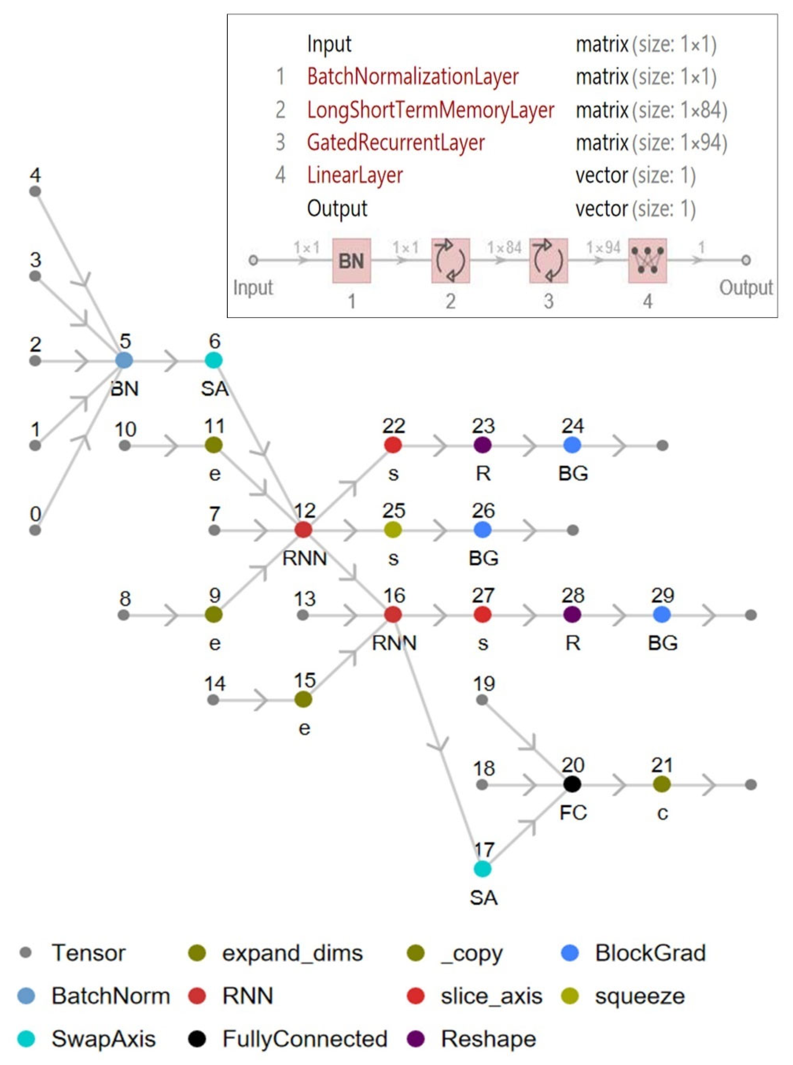
2.2. An Overview of GRU and LSTM
2.2.1. Gated Recurrent Unit (GRU)
2.2.2. Long Short-Term Memory (LSTM)
3. Performance Evaluation
4. Results
5. Discussion
6. Conclusions
Author Contributions
Funding
Institutional Review Board Statement
Informed Consent Statement
Data Availability Statement
Acknowledgments
Conflicts of Interest
References
- Alzate-Arias, S.; Jaramillo-Duque, Á.; Villada, F.; Restrepo-Cuestas, B. Assessment of Government Incentives for Energy from Waste in Colombia. Sustainability 2018, 10, 1294. [Google Scholar] [CrossRef]
- Rajaeifar, M.A.; Ghanavati, H.; Dashti, B.B.; Heijungs, R.; Aghbashlo, M.; Tabatabaei, M. Electricity generation and GHG emission reduction potentials through different municipal solid waste management technologies: A comparative review. Renew. Sustain. Energy Rev. 2017, 79, 414–439. [Google Scholar] [CrossRef]
- Ibrahim, O.; Al-Kindi, G.; Qureshi, M.U.; Maghawry, S.A. Challenges and Construction Applications of Solid Waste Management in Middle East Arab Countries. Processes 2022, 10, 2289. [Google Scholar] [CrossRef]
- Qazi, W.A.; Abushammala, M.F.M. The analysis of electricity production and greenhouse-gas emission reduction from municipal solid waste sector in Oman. Int. J. Environ. Sci. Technol. 2020, 18, 1395–1406. [Google Scholar] [CrossRef]
- Hou, D.; Song, Y.; Zhang, J.; Hou, M.; O’Connor, D.; Harclerode, M. Climate change mitigation potential of contaminated land redevelopment: A city-level assessment method. J. Clean. Prod. 2018, 171, 1396–1406. [Google Scholar] [CrossRef]
- Dong, H.; Zhang, L. Transition towards carbon neutrality: Forecasting Hong Kong’s buildings carbon footprint by 2050 using a machine learning approach. Sustain. Prod. Consum. 2023, 35, 633–642. [Google Scholar] [CrossRef]
- Dagar, V.; Khan, M.K.; Alvarado, R.; Usman, M.; Zakari, A.; Rehman, A.; Murshed, M.; Tillaguango, B. Variations in technical efficiency of farmers with distinct land size across agro-climatic zones: Evidence from India. J. Clean. Prod. 2021, 315, 128109. [Google Scholar] [CrossRef]
- Mardani, A.; Liao, H.; Nilashi, M.; Alrasheedi, M.; Cavallaro, F. A multi-stage method to predict carbon dioxide emissions using dimensionality reduction, clustering, and machine learning techniques. J. Clean. Prod. 2020, 275, 122942. [Google Scholar] [CrossRef]
- Cui, Y.; Su, W.; Xing, Y.; Hao, L.; Sun, Y.; Cai, Y. Experimental and simulation evaluation of CO2/CO separation under different component ratios in blast furnace gas on zeolites. Chem. Eng. J. 2023, 472, 144579. [Google Scholar] [CrossRef]
- Ahmad, M.; Jiang, P.; Murshed, M.; Shehzad, K.; Akram, R.; Cui, L.; Khan, Z. Modelling the dynamic linkages between eco-innovation, urbanization, economic growth and ecological footprints for G7 countries: Does financial globalization matter? Sustain. Cities Soc. 2021, 70, 102881. [Google Scholar] [CrossRef]
- Xu, X.; Liao, M. Prediction of Carbon Emissions in China’s Power Industry Based on the Mixed-Data Sampling (MIDAS) Regression Model. Atmosphere 2022, 13, 423. [Google Scholar] [CrossRef]
- Bakır, H.; Ağbulut, Ü.; Gürel, A.E.; Yıldız, G.; Güvenç, U.; Soudagar, M.E.M.; Hoang, A.T.; Deepanraj, B.; Saini, G.; Afzal, A. Forecasting of future greenhouse gas emission trajectory for India using energy and economic indexes with various metaheuristic algorithms. J. Clean. Prod. 2022, 360, 131946. [Google Scholar] [CrossRef]
- Iftikhar, H.; Khan, M.; Żywiołek, J.; Khan, M.; López-Gonzales, J.L. Modeling and forecasting carbon dioxide emission in Pakistan using a hybrid combination of regression and time series models. Heliyon 2024, 10, e33148. [Google Scholar] [CrossRef] [PubMed]
- Abushammala, M.F.; Qazi, W.A.; Azam, M.-H.; Mehmood, U.A.; Al-Mufragi, G.A.; Alrawahi, N.-A. Economic and environmental benefits of landfill gas utilisation in Oman. Waste Manag. Res. 2016, 34, 717–723. [Google Scholar] [CrossRef]
- Alsabbagh, M. Mitigation of CO2e Emissions from the Municipal Solid Waste Sector in the Kingdom of Bahrain. Climate 2019, 7, 100. [Google Scholar] [CrossRef]
- Zhang, F.; Deng, X.; Xie, L.; Xu, N. China’s energy-related carbon emissions projections for the shared socioeconomic pathways. Resour. Conserv. Recycl. 2021, 168, 105456. [Google Scholar] [CrossRef]
- NASA. Carbon Dioxide. NASA, May 2024. Available online: https://climate.nasa.gov/vital-signs/carbon-dioxide/?intent=121 (accessed on 27 June 2024).
- Li, G.; Chen, X.; You, X.-Y. System dynamics prediction and development path optimization of regional carbon emissions: A case study of Tianjin. Renew. Sustain. Energy Rev. 2023, 184, 113579. [Google Scholar] [CrossRef]
- Qader, M.R.; Khan, S.; Kamal, M.; Usman, M.; Haseeb, M. Forecasting carbon emissions due to electricity power generation in Bahrain. Environ. Sci. Pollut. Res. 2022, 29, 17346–17357. [Google Scholar] [CrossRef]
- Li, Z.; Gan, B.; Li, Z.; Zhang, H.; Wang, D.; Zhang, Y.; Wang, Y. Kinetic mechanisms of methane hydrate replacement and carbon dioxide hydrate reorganization. Chem. Eng. J. 2023, 477, 146973. [Google Scholar] [CrossRef]
- Li, J.; Zhang, Q.; Etienne, X.L. Optimal carbon emission reduction path of the building sector: Evidence from China. Sci. Total Environ. 2024, 919, 170553. [Google Scholar] [CrossRef]
- Liu, X.; Wang, X.; Meng, X. Carbon Emission Scenario Prediction and Peak Path Selection in China. Energies 2023, 16, 2276. [Google Scholar] [CrossRef]
- Matthews, H.D.; Caldeira, K. Transient climate–carbon simulations of planetary geoengineering. Proc. Natl. Acad. Sci. USA 2007, 104, 9949–9954. [Google Scholar] [CrossRef] [PubMed]
- Hosseini, S.M.; Saifoddin, A.; Shirmohammadi, R.; Aslani, A. Forecasting of CO2 emissions in Iran based on time series and regression analysis. Energy Rep. 2019, 5, 619–631. [Google Scholar] [CrossRef]
- Xu, M.; Zhang, J.; Li, Z. A novel Lasso-ARMA model for time series prediction. In Proceedings of the Chinese Automation Congress (CAC), Xi’an, China, 30 November–2 December 2018. [Google Scholar] [CrossRef]
- Ibrahim, O.; AlMaghawry, S. Review on Cyclone Shaheen in the Sultanate of Oman. Arab. J. Geosci. 2022, 15, 1. [Google Scholar]
- Ibrahim, O.R.; AlMaghawry, S.; AlAmir, M. Tracking the damages of Shaheen cyclone in the Sultanate of Oman. Water Pract. Technol. 2022, 17, 2548–2553. [Google Scholar] [CrossRef]
- Ibrahim, O.R.; Maghawry, S.A. A comparative analysis of precipitation estimates of cyclone Shaheen and Al Azm trough using GPM-based near-real-time satellite. Arab. J. Geosci. 2024, 17, 1–13. [Google Scholar] [CrossRef]
- Zafar, S. Municipal Solid Waste Management in Oman. 20 March 2022. Available online: https://www.bioenergyconsult.com/msw-oman/ (accessed on 15 December 2022).
- Charabi, Y.; Al-Awadhi, T.; Choudri, B.S. Strategic pathways and regulatory choices for effective GHG reduction in hydrocarbon based economy: Case of Oman. Energy Rep. 2018, 4, 653–659. [Google Scholar] [CrossRef]
- Yu, B.; Chen, Q.; Li, N.; Wang, Y.; Li, L.; Cai, M.; Zhang, W.; Gu, T.; Zhu, R.; Zeng, H.; et al. Life cycle assessment of urban road networks: Quantifying carbon footprints and forecasting future material stocks. Constr. Build. Mater. 2024, 428, 136280. [Google Scholar] [CrossRef]
- Fang, K.; Li, C.; Tang, Y.; He, J.; Song, J. China’s pathways to peak carbon emissions: New insights from various industrial sectors. Appl. Energy 2022, 306, 118039. [Google Scholar] [CrossRef]
- Prabhu, C. Oman Has Committed to Reducing Its Greenhouse Gas Emissions by 2% by the Year 2030. Oman Observer, 24 September 2019. Available online: https://www.omanobserver.om/article/24102/Business/oman-not-immune-to-impacts-of-global-climate-change (accessed on 28 June 2024).
- Mason, K.; Duggan, J.; Howley, E. Forecasting energy demand, wind generation and carbon dioxide emissions in Ireland using evolutionary neural networks. Energy 2018, 155, 705–720. [Google Scholar] [CrossRef]
- Tian, Y.; Xiong, S.; Ma, X.; Ji, J. Structural path decomposition of carbon emission: A study of China’s manufacturing industry. J. Clean. Prod. 2018, 193, 563–574. [Google Scholar] [CrossRef]
- Ye, L.; Du, P.; Wang, S. Industrial carbon emission forecasting considering external factors based on linear and machine learning models. J. Clean. Prod. 2024, 434, 140010. [Google Scholar] [CrossRef]
- Chen, H.; Wang, R.; Liu, X.; Du, Y.; Yang, Y. Monitoring the enterprise carbon emissions using electricity big data: A case study of Beijing. J. Clean. Prod. 2023, 396, 136427. [Google Scholar] [CrossRef]
- Li, Y. Forecasting Chinese carbon emissions based on a novel time series prediction method. Energy Sci. Eng. 2020, 8, 2274–2285. [Google Scholar] [CrossRef]
- Auffhammer, M.; Carson, R.T. Forecasting the path of China’s CO2 emissions using province-level information. J. Environ. Econ. Manag. 2008, 55, 229–247. [Google Scholar] [CrossRef]
- Costantini, L.; Laio, F.; Mariani, M.S.; Ridolfi, L.; Sciarra, C. Forecasting national CO2 emissions worldwide. Sci. Rep. 2024, 14, 22438. [Google Scholar] [CrossRef]
- Li, F.; Sun, M.; Xian, Q.; Feng, X. MDL: Industrial carbon emission prediction method based on meta-learning and diff long short-term memory networks. PLoS ONE 2024, 19, e0307915. [Google Scholar] [CrossRef]
- Jena, P.R.; Managi, S.; Majhi, B. Forecasting the CO2 emissions at the global level: A multilayer artificial neural network modelling. Energies 2021, 14, 6336. [Google Scholar] [CrossRef]
- Kumari, S.; Singh, S.K. Machine learning-based time series models for effective CO2 emission prediction in India. Environ. Sci. Pollut. Res. 2023, 30, 116601–116616. [Google Scholar] [CrossRef]
- Hannah, R.; Rosado, P.; Roser, M. CO2 and Greenhouse Gas Emissions. 2023. Available online: https://ourworldindata.org/co2-and-greenhouse-gas-emissions (accessed on 5 December 2023).
- Linardatos, P.; Papastefanopoulos, V.; Panagiotakopoulos, T.; Kotsiantis, S. CO2 concentration forecasting in smart cities using a hybrid ARIMA–TFT model on multivariate time series IoT data. Sci. Rep. 2023, 13, 17266. [Google Scholar] [CrossRef]
- Rajmohan, R.; Pavithra, M.; Kumar, T.A.; Manjubala, P. Exploration of deep RNN architectures: LSTM and gru in medical diagnostics of cardiovascular and neuro diseases. In Handbook of Deep Learning in Biomedical Engineering and Health Informatics; Apple Academic Press: Palm Bay, FL, USA, 2021; pp. 167–202. [Google Scholar]
- Nosouhian, S.; Nosouhian, F.; Khoshouei, A.K. A Review of Recurrent Neural Network Architecture for Sequence Learning: Comparison Between LSTM and GRU. 2021. Available online: https://www.preprints.org/frontend/manuscript/3fa37c0d5d54bea69f5b855f25306b5e/download_pub (accessed on 12 July 2021).
- Doshi, K. Batch Norm Explained Visually—How It Works, and Why Neural Networks Need It. Medium. 2022. Available online: https://towardsdatascience.com/batch-norm-explained-visually-how-it-works-and-why-neural-networks-need-it-b18919692739/ (accessed on 9 June 2024).
- Al-kahtani, M.S.; Mehmood, Z.; Sadad, T.; Zada, I.; Ali, G.; ElAffendi, M. Intrusion detection in the Internet of Things using fusion of GRU-LSTM deep learning model. Intell. Autom. Soft Comput. 2023, 37, 2279–2290. [Google Scholar] [CrossRef]
- Islam, M.S.; Hossain, E. Foreign exchange currency rate prediction using a GRU-LSTM hybrid network. Soft Comput. Lett. 2021, 3, 100009. [Google Scholar] [CrossRef]
- Sherstinsky, A. Fundamentals of recurrent neural network (RNN) and long short-term memory (LSTM) network. Phys. D Nonlinear Phenom. 2020, 404, 132306. [Google Scholar] [CrossRef]
- Bulin, J.; Hamaekers, J. Similarity of particle systems using an invariant root mean square deviation measure. arXiv 2021, arXiv:2106.09363. [Google Scholar]
- Chicco, D.; Warrens, M.J.; Jurman, G. The coefficient of determination R-squared is more informative than SMAPE, MAE, MAPE, MSE and RMSE in regression analysis evaluation. PeerJ Comput. Sci. 2021, 7, e623. [Google Scholar] [CrossRef]
- Tseng, S.-H.; Wang, C.-H.; Duong, T.H.T. Neural Network Prediction Model–Applied to US Industrial Greenhouse Gas Emissions. Arch. Environ. Prot. 2025, 51, 103–115. [Google Scholar] [CrossRef]
- Sha, M.; Emmanuel, S.; Bindhu, A.; Mustaq, M. Intensified greenhouse gas prediction: Configuring Gate with Fine-Tuning Shifts with Bi-LSTM and GRU System. Front. Clim. 2024, 6, 1457441. [Google Scholar] [CrossRef]
- Caneo, J.; Scavia, J.; Minutolo, M.C.; Kristjanpoller, W. A hybrid model to forecast greenhouse gas emissions in latin america. Soft Comput. 2023, 27, 17943–17970. [Google Scholar] [CrossRef]
- Wang, Q.; Li, S.; Pisarenko, Z. Modeling carbon emission trajectory of China, US and India. J. Clean. Prod. 2020, 258, 120723. [Google Scholar] [CrossRef]
- Zhao, Y.; Yang, L.; Pan, H.; Li, Y.; Shao, Y.; Li, J.; Xie, X. Spatio-temporal prediction of groundwater vulnerability based on CNN-LSTM model with self-attention mechanism: A case study in Hetao Plain, northern China. J. Environ. Sci. 2025, 153, 128–142. [Google Scholar] [CrossRef]
- Kong, Y.; Wang, Z.; Nie, Y.; Zhou, T.; Zohren, S.; Liang, Y.; Sun, P.; Wen, Q. Unlocking the power of lstm for long term time series forecasting. arXiv 2024, arXiv:2408.10006. [Google Scholar] [CrossRef]
- Zhao, X.; Han, M.; Ding, L.; Calin, A.C. Forecasting carbon dioxide emissions based on a hybrid of mixed data sampling regression model and back propagation neural network in the USA. Environ. Sci. Pollut. Res. 2018, 25, 2899–2910. [Google Scholar] [CrossRef] [PubMed]
- Shakiru, T.H.; Liu, X.; Liu, Q. A hybrid Modeling and Forecasting of Carbon dioxide Emissions in Tanzania. Gen. Lett. Math. GLM 2023, 13, 5–17. [Google Scholar] [CrossRef]


| Industry | Statistical Characteristics | CO2 (Tonnes per Person) |
|---|---|---|
| Annual | Min | 0.01 |
| Max | 17.79 | |
| Mean | 9.11 | |
| Zero number | 0 | |
| Variance | 29.67 | |
| Skewness | 0.03 | |
| Count | 59 | |
| Oil | Min | 0 |
| Max | 6.96 | |
| Mean | 2.27 | |
| Zero number | 1 | |
| Variance | 2.14 | |
| Skewness | 0.53 | |
| Count | 59 | |
| Gas | Min | 0 |
| Max | 12.42 | |
| Mean | 4.78 | |
| Zero number | 15 | |
| Variance | 19.64 | |
| Skewness | 0.54 | |
| Count | 59 | |
| Cement | Min | 0 |
| Max | 0.59 | |
| Mean | 0.22 | |
| Zero number | 21 | |
| Variance | 0.04 | |
| Skewness | 0.24 | |
| Count | 59 | |
| Flaring | Min | 0 |
| Max | 8.72 | |
| Mean | 1.81 | |
| Zero number | 7 | |
| Variance | 3.55 | |
| Skewness | 2.38 | |
| Count | 59 |
| Type of Parameters | Values/Layer |
|---|---|
| Network Type | Feed-forward propagation |
| Data Division | Train (70%) Test (30%) |
| Number of Hidden layers (Neurons) | 10–45 |
| Batch Size | 34–210 |
| learning Function | 0.01–0.027 |
| Activation Function | Ramp, Logistic |
| Normalization Function | Batch Normalization |
| Training function | Adam |
| Scenario | Input | Output | |||
|---|---|---|---|---|---|
| M1 | Oil | Annual CO2 | |||
| M2 | Oil | Gas | Annual CO2 | ||
| M3 | Oil | Gas | Cement | Annual CO2 | |
| M4 | Oil | Gas | Cement | Flaring | Annual CO2 |
| Parameter | Testing | |||
|---|---|---|---|---|
| Model | R | RMSE (Tonnes per Person) | MAPE (Tonnes per Person) | |
| Annual CO2 | LSTM-GRU-M1 | 0.881 | 5.129 | 31.034 |
| LSTM-GRU-M2 | 0.891 | 3.259 | 19.603 | |
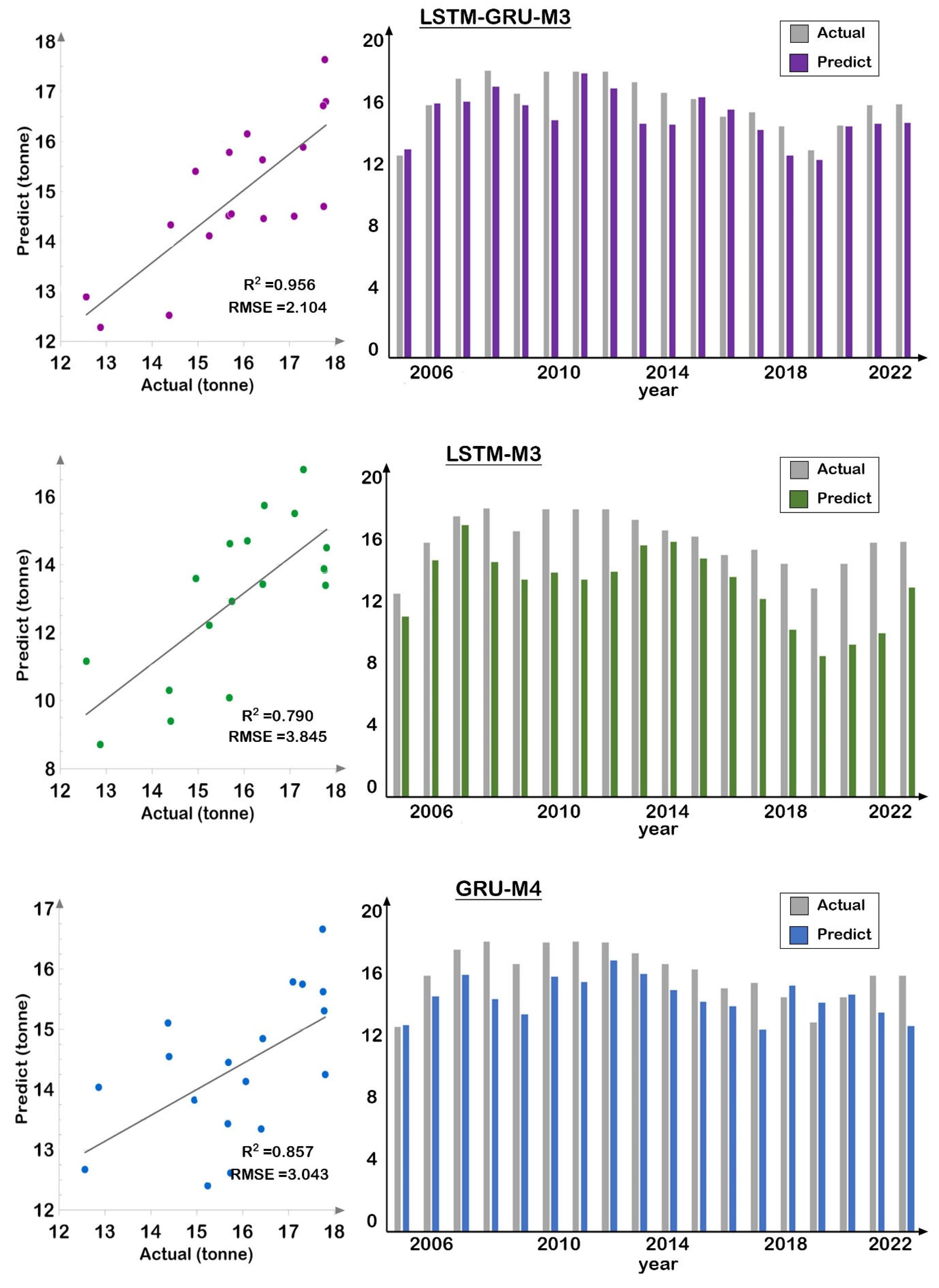
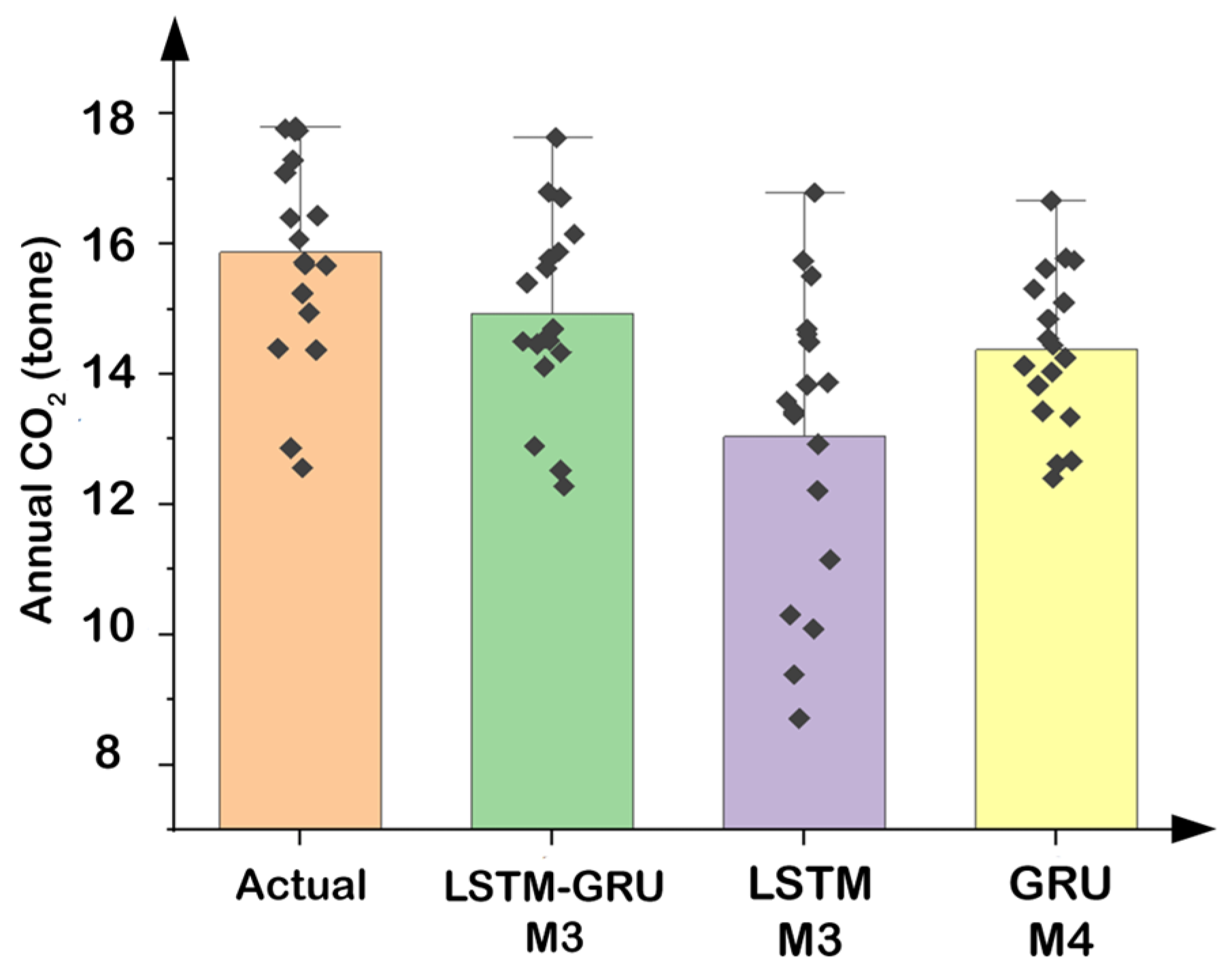
| LSTM-GRU-M3 | 0.978 | 2.104 | 11.876 | |
| LSTM-GRU-M4 | 0.934 | 2.777 | 16.487 | |
| LSTM-M1 | 0.859 | 6.393 | 38.748 | |
| LSTM-M2 | 0.881 | 4.615 | 27.064 | |
| LSTM-M3 | 0.889 | 3.845 | 23.232 | |
| LSTM-M4 | 0.886 | 3.994 | 24.032 | |
| GRU-M1 | 0.852 | 5.926 | 35.644 | |
| GRU-M2 | 0.887 | 3.972 | 24.062 | |
| GRU-M3 | 0.909 | 3.285 | 19.069 | |
| GRU-M4 | 0.926 | 3.043 | 16.867 | |
Disclaimer/Publisher’s Note: The statements, opinions and data contained in all publications are solely those of the individual author(s) and contributor(s) and not of MDPI and/or the editor(s). MDPI and/or the editor(s) disclaim responsibility for any injury to people or property resulting from any ideas, methods, instructions or products referred to in the content. |
© 2025 by the authors. Licensee MDPI, Basel, Switzerland. This article is an open access article distributed under the terms and conditions of the Creative Commons Attribution (CC BY) license (https://creativecommons.org/licenses/by/4.0/).
Share and Cite
Wang, C.; Zhang, X.; Nie, Z.; Gajbhiye Meshram, S. Prediction of Annual Carbon Emissions Based on Carbon Footprints in Various Omani Industries to Draw Reduction Paths with LSTM-GRU Hybrid Model. Sustainability 2025, 17, 4940. https://doi.org/10.3390/su17114940
Wang C, Zhang X, Nie Z, Gajbhiye Meshram S. Prediction of Annual Carbon Emissions Based on Carbon Footprints in Various Omani Industries to Draw Reduction Paths with LSTM-GRU Hybrid Model. Sustainability. 2025; 17(11):4940. https://doi.org/10.3390/su17114940
Chicago/Turabian StyleWang, Chen, Xiaomin Zhang, Zekai Nie, and Sarita Gajbhiye Meshram. 2025. "Prediction of Annual Carbon Emissions Based on Carbon Footprints in Various Omani Industries to Draw Reduction Paths with LSTM-GRU Hybrid Model" Sustainability 17, no. 11: 4940. https://doi.org/10.3390/su17114940
APA StyleWang, C., Zhang, X., Nie, Z., & Gajbhiye Meshram, S. (2025). Prediction of Annual Carbon Emissions Based on Carbon Footprints in Various Omani Industries to Draw Reduction Paths with LSTM-GRU Hybrid Model. Sustainability, 17(11), 4940. https://doi.org/10.3390/su17114940