Article

Explaining Urban Vitality Through Interpretable Machine Learning: A Big Data Approach Using Street View Images and Environmental Factors

1
School of Geomatics and Urban Spatial Informatics, Beijing University of Civil Engineering and Architecture, Beijing 102616, China
2
Research Center for Urban Big Data Applications, Beijing University of Civil Engineering and Architecture, Beijing 100044, China
*
Author to whom correspondence should be addressed.
Sustainability 2025, 17(11), 4926; https://doi.org/10.3390/su17114926
Submission received: 18 March 2025 / Revised: 22 May 2025 / Accepted: 23 May 2025 / Published: 27 May 2025
(This article belongs to the Special Issue Socially Sustainable Urban and Architectural Design)

Abstract

:
Urban vitality (UV) is a critical indicator for measuring the level of sustainable urban development, closely associated with environmental factors such as population density, economic activity, and spatial utilization efficiency. However, traditional methods face significant limitations in capturing the heterogeneity and nonlinear relationships between urban vitality and its influencing factors. This study suggests an interpretable machine learning framework to address the aforementioned issues. It combines a gradient boosting decision tree (GBDT) model with the SHapley Additive exPlanation (SHAP) framework to examine the urban vitality distribution characteristics and factors that influence them in Beijing’s fifth ring road. The main findings include the following: Urban vitality within Beijing’s fifth ring road exhibits significant spatial clustering and positive correlations, with clear spatial heterogeneity. The plot ratio (PR) exerts a notable positive influence on urban vitality, while green space accessibility (DG) demonstrates the strongest negative impact. The building density (BD), in contrast, shows a strong negative correlation with urban vitality. Variables such as the NDVI, average housing price (AHP), and road network density (RND) contribute significantly to urban vitality, reflecting the combined effects of vegetation coverage, economic conditions, and transportation layout. The findings provide a quantitative analytical tool for urban planning, facilitating resource optimization, improving urban vitality, and supporting scientific and rational decision-making.

1. Introduction

1.1. Introduction to Urban Vitality

Urban vitality is becoming more widely acknowledged as a crucial component in directing sustainable urban growth and planning, and it is a significant measure of a city’s level of vibrancy and livability. The term “urban vitality” was first used by Jacobs [1], who described it as “street life over a 24-h period”. Since then, researchers from a variety of academic fields, including urban sociology and urban morphology, have progressively expanded on the definition of urban vitality [2]. It is widely accepted that the “concentration of people” is the fundamental component of urban life, despite the fact that different experts’ formulations emphasize different elements [3]. In addition to showcasing a city’s appeal and competitiveness, a bustling urban area is essential for raising citizens’ standards of living and fostering the city’s sustainable growth [4]. Therefore, creating a vibrant and great urban and rural living environment is one of the primary objectives of Chinese urban development and planning [5].

1.2. Evolution of Urban Vitality Measurement

At this point, researchers have been concentrating on the dynamic patterns of human activity in space, as well as the geographical and temporal distribution aspects of urban life. Early measures of urban vitality relied mostly on methods such as participatory observation, and these studies usually focused on small-scale areas such as neighborhoods to analyze local urban vitality [6]. However, due to the limited sample size, it is difficult for these methods to comprehensively reveal the characteristics of urban vitality in large-scale areas and over long time periods [7]. Real-time recording of inhabitants’ activities and location information has been made possible by the growth of information and communication technology (ICT) with the emergence of a smart society [8]. These highly spatially and temporally accurate large-scale Volunteered Geographic Information (VGI) datasets open up new avenues for researching the spatial features of urban vitality and how it evolves over vast regions. Rich data support for in-depth research on urban vitality has been made possible by the widespread use of GPS data [9,10], location service data [11], point-of-interest data [12], social media check-in information [13], restaurant review data [14,15], Wi-Fi hotspot data [16], traffic card swipe data [17], Baidu heat maps [18], mobile phone signaling data [19], and particularly street view data to measure the intensity of activities in spatial units.
Based on the assessment of urban vitality, researchers have been investigating the effects of built environment features on urban vitality. Conventional research approaches use regression models (e.g., least squares) to examine how built environment elements like land-use diversity, population density, and transportation accessibility affect urban vitality globally [20]. Although the relationship between the physical environment and urban vitality has been originally demonstrated by these studies, it is frequently challenging to offer practical recommendations for actual urban planning and management because of methodological limitations and study assumptions [21]. Empirical studies have shown that moderate development intensity, diversified land use and facility allocation, and well-designed pedestrian environments can help enhance urban vitality. However, there are also studies that point out that excessive development and land-use diversification can lead to overcrowded spaces and impose psychological burdens on residents, thus inhibiting urban vitality [22]. These differences may stem from factors such as the research environments, definitions of variables, and measurement methods in different regions, but more importantly, many of the global relationships assumed in the studies may not be applicable to each region, leading to inconsistent results. Some studies have employed regionally weighted regression models, accounting for the spatial dependency of urban vitality, to examine the local effects of built environment elements on urban vitality at different spatial scales. This offers a fresh viewpoint on comprehending the features of spatially differentiated urban vitality [23].

1.3. The Need for Nonlinear Modeling and Interpretability

As machine learning and other cutting-edge techniques have gradually matured in recent years [24,25,26], they have become increasingly popular in the research of locals’ travel habits [27]. The impact of the built environment (BE) on residents’ travel behavior has a nonlinear marginal characteristic and is usually only noticeable within a specific range of values or magnitude of change, as research has shown that there is a threshold effect and a significant nonlinear relationship between the two [28]. Given that travel behavior is fundamentally about satisfying inhabitants’ desires to get to their destinations in order to engage in particular activities, the relationship between urban vitality and the BE is probably going to share comparable nonlinear properties and threshold effects. For example, increasing the intensity of urban development within a reasonable range may contribute significantly to urban vitality, but once a certain threshold is exceeded, the marginal effect may diminish or even become inhibitory. At the theoretical and methodological level, the study of nonlinear and threshold effects reveals the local characteristics of the built environment’s impact on urban vitality from the perspective of marginal effects, further questioning the universal assumption of a global relationship between the two [29]. At the application level, the empirical analyses of nonlinear and threshold effects, especially the relative importance of each built environment element on urban vitality, its effective range of action, and the nonlinear variation of marginal effects, can provide efficient guidance for the precise planning and governance of the built environment, thus enhancing the level of urban vitality more effectively. Recent advances in machine learning have therefore opened up new avenues for modelling such complex relationships [30].

1.4. The Black Box Challenge: Towards Interpretable Machine Learning

While machine learning models, especially ensemble methods such as random forests and deep learning models such as neural networks, show great promise in predicting urban vitality, their ‘black box’ nature often limits their interpretability [31,32]. The lack of transparency in the decision-making process poses a great challenge to urban planners and policy-makers, who need to have a clear understanding of how environmental factors affect urban vitality in order to make effective decisions [33]. To address this problem, there is a growing demand for interpretable machine learning techniques that not only capture the intricate and nonlinear relationships between environmental factors and urban vitality, but also provide clear and actionable insights [34]. Among these techniques, Shapley values derived from cooperative game theory have emerged as a powerful tool for model interpretability. By attributing each environmental factor’s individual contribution to the final prediction, the model Shapley values provide a transparent and consistent way to understand the impact of each feature in the model [35].

1.5. Research Objectives and Contributions

In summary, current research on the nonlinear effects of the built environment on urban vitality still faces the following major problems: (1) the selection of built environment factors that affect urban vitality is relatively limited; (2) the nonlinear relationship between environmental factors and urban vitality is difficult to be quantified and accurately captured; and (3) the existing models lack the means of visual interpretation in this direction. Therefore, the study of visualizing and explaining the nonlinear effects of environmental factors on urban vitality has not yet been conducted in depth, especially in identifying the dominant drivers and their mechanisms of action, which still need to be further explored. Specifically, there is an urgent need to answer the following core questions: (1) Which major environmental factors dominate in relative importance (RI)? How are they ranked in terms of their contribution to urban vitality? (2) How can the nonlinear relationship between urban vitality and environmental elements be quantified and explained? (3) How can urban vitality’s crucial function in urban development be properly enhanced? The following outcomes are the main emphasis of this study in order to address the aforementioned questions:
(1)
Urban vitality measurement and spatial correlation analysis: Using Beijing’s fifth ring road as the research region, we compute the urban vitality values there and do a thorough examination of its spatial distribution features and correlations using the ResNet50 model, which was trained using the Place Pulse 2.0 dataset.
(2)
Modeling of nonlinear relationships and exploration of threshold effects: Cross-validation is used to optimize the hyperparameters and construct the optimal GBDT model, which provides high-precision data support for the exploration of the nonlinear correlation between environmental data and urban vitality and the threshold effect.
(3)
To determine the dominating components and quantify their respective contributions to urban vitality, an interpretation framework based on SHAP was presented. This framework was used to compute the RIs of environmental factors using the global SHAP values.
(4)
Local interpretation and visualization: Using the Local Dependence Plots (LDPs) of SHAP, the SHAP values of the environmental data for each urban vitality factor were visually presented, thus revealing the nonlinear relationship and threshold characteristics between the environmental factors and the urban vitality.
Compared to traditional approaches that rely on static demographic, economic, or land-use indicators, the proposed method introduces a perceptual and data-driven framework for capturing urban vitality. By leveraging street-level imagery and deep learning (ResNet50), this study quantifies the visual liveliness of urban scenes, reflecting how residents and visitors may experience the urban environment. In addition, the use of the SHAP interpretability framework enables the analysis of complex, nonlinear relationships between environmental features and perceived vitality, which are often overlooked in regression-based or index-based models. This integrated approach offers improved spatial granularity, greater scalability, and enhanced explanatory power, thereby addressing key limitations of conventional urban vitality assessments.
The article is organized in a structured manner comprising five key sections. Section 2 encompasses the geographical context of the study area, experimental dataset details, and data processing methodologies. Section 3 presents the overarching research framework and methodological approach employed throughout the investigation. The key findings and expectations are covered in Section 4. The primary findings and anticipated outcomes are thoroughly discussed in Section 5. Finally, Section 6 provides a concise summary of the research, acknowledges limitations, and outlines future research directions.

2. Study Area and Materials

2.1. Study Area

The topography of Beijing creates a multi-layered spatial pattern where farms in the plains outside the city, ecological land on the outskirts of the city, and the city center are alternately distributed. This topographic feature has created a distinctive landscape where the city’s economic and ecological activities are linked. By using the fifth ring road as a core, we can more effectively concentrate on high-intensity urban development zones and examine how traffic, population, and economic factors influence the spatial pattern of urban vitality. As illustrated in Figure 1, the region encompasses the city’s main built-up areas and functional core areas, with an emphasis on Beijing’s political, economic, cultural, and ecological roles as the capital. The objective of this research is to enable the development of a more dynamic and resilient urban environment by offering a scientific foundation for urban management and optimization.

2.2. Data

To guarantee thorough analysis, this study used a range of data sources:
(1) OpenStreetMap (https://www.openstreetmap.org/, accessed on 21 May 2025) was used to extract data on urban road networks; (2) Python (Version 3.8) scripts were used to gather street view imagery in bulk from Baidu Street View Map (https://map.baidu.com/, accessed on 21 May 2025); (3) land-use data came from the Resource and Environment Data Center of the Chinese Academy of Sciences (https://www.resdc.cn/, accessed on 21 May 2025); (4) NDVI computations used Landsat 8 multispectral remote sensing images (https://www.gscloud.cn/, accessed on 21 May 2025); (5) urban green space coverage data came from the European Space Agency’s Global Land Cover Data 2020 report (https://www.esa.int/, accessed on 21 May 2025); (6) POI data for parks and settlements were crawled from Baidu Maps (https://map.baidu.com/, accessed on 21 May 2025); (7) housing age and price information came from the Lianjia real estate platform (https://bj.lianjia.com/, accessed on 21 May 2025); and (8) population density data were provided by the WorldPop platform (https://www.worldpop.org/, accessed on 21 May 2025).
The data used in this article are from 2020 and these diverse data sources ensured a robust foundation for the study, facilitating detailed spatial and temporal analysis of urban characteristics.

2.3. The Place Pulse 2.0 Dataset

This dataset is designed for studying human perceptions of urban environments [36]. It was developed as part of research to analyze how different urban features impact people’s feelings and judgments about a place’s characteristics [37]. The dataset provides a unique combination of street view images and crowd-sourced human annotations, making it a valuable resource for urban studies, computer vision, and social sciences. Human perception data were collected through an online game-like interface, where participants were asked to compare two images based on predefined attributes. These annotations reflect how people perceive and evaluate urban spaces. Participants compared images in a binary choice format (e.g., “Which place looks lively?”), generating scores for each location based on aggregated votes [38]. The dataset is large and geographically extensive, making it suitable for training machine learning models to predict urban perceptions, analyze urban planning outcomes, and study the relationship between environment data and urban vitality.

2.4. Street View Images of Beijing

Using a Python script, coordinates were entered via the Baidu Street View API to acquire street view photos. In the research region, points were placed at 50 m intervals, yielding 29,940 sample points in total. At least six perspectives were used to take Street View pictures at each location, and six more were added for specific locations where panoramic pictures could not be produced. Therefore, in order to create a 360-degree, non-overlapping panorama that is 2048 pixels wide and 664 pixels high, we stitched the street view images together using OpenCV (Version 4.2.0)’s Replcher algorithm. Since each panoramic image is a circular view, it is more suited to human vision.

2.5. Variables

2.5.1. Built Environment Data

The built environment is the exterior urban space that has been created, altered, and modified to accommodate human activity. It covers multi-dimensional interactive elements such as land use, transport infrastructure, urban design, etc., and provides support space for human social activities. From the perspective of urban vitality, the built environment significantly shapes the level of vitality of a city through its influence on population activities, resource distribution, and functional connectivity. Based on the widely used ‘5D’ framework (Density, Design, Diversity, Distance, and Connectivity) [39], this paper selects 11 built environment variables as important influences on urban vitality, as shown in Table 1. These variables comprehensively reflect the multi-dimensional characteristics of the built environment in terms of spatial structure, resource allocation, and functional connectivity. Figure 2 illustrates the selected environmental variables in this paper, and by quantifying the spatial distribution characteristics of these variables, it provides reliable basic data for an in-depth study of the mechanism of the built environment’s effect on urban vitality.

2.5.2. Socioeconomic Data

Regarding socioeconomic factors, the average house price was chosen and computed based on prior research. Finally, using ArcGIS (Version 10.8)’s Zoning Statistics and Spatial Connectivity Toolbox, all spatial data were merged into grid cells of 500 m by 500 m, as was commonly done in previous studies. A total of 2551 grid cells were tallied in this study region.

3. Methodology

3.1. Overview of the Framework

By carefully examining the degree of urban vitality, this research undertakes a methodical investigation grounded in a clearly defined conceptual and analytical framework. Based on this definition, the analytical workflow is divided into three major stages, and this study design and workflow are shown in Figure 3:
(1)
Defining variables and computing urban vitality
Urban vitality can be operationalized as the perception of urban spatial vitality, derived from human perception data. In this study, the Place Pulse 2.0 dataset, which captures subjective perceptions of urban scenes, was used to train the ResNet50 deep learning model, and the model was used to extract image features related to the perception of vitality from Beijing’s street view images (see Section 2.3 and Section 3.2 for details). These features are aggregated to generate an urban vitality score for each spatial unit.
(2)
Modeling nonlinear associations and interpreting results
A gradient boosting decision tree (GBDT) model is trained to explore the nonlinear relationships between urban vitality and various environmental and spatial features. To ensure transparency, a SHAP-based interpretability framework is applied to identify and visualize the contribution of each input feature. Optimal GBDT parameters are selected through grid search and K-fold cross-validation to ensure robustness.
(3)
Model validation and spatial analysis
The accuracy of the GBDT model is evaluated using standard performance metrics. In addition, spatial autocorrelation analysis is conducted to assess clustering patterns in urban vitality. The SHAP framework is further used to explain how specific built environment factors influence the vitality outcomes in different urban contexts.

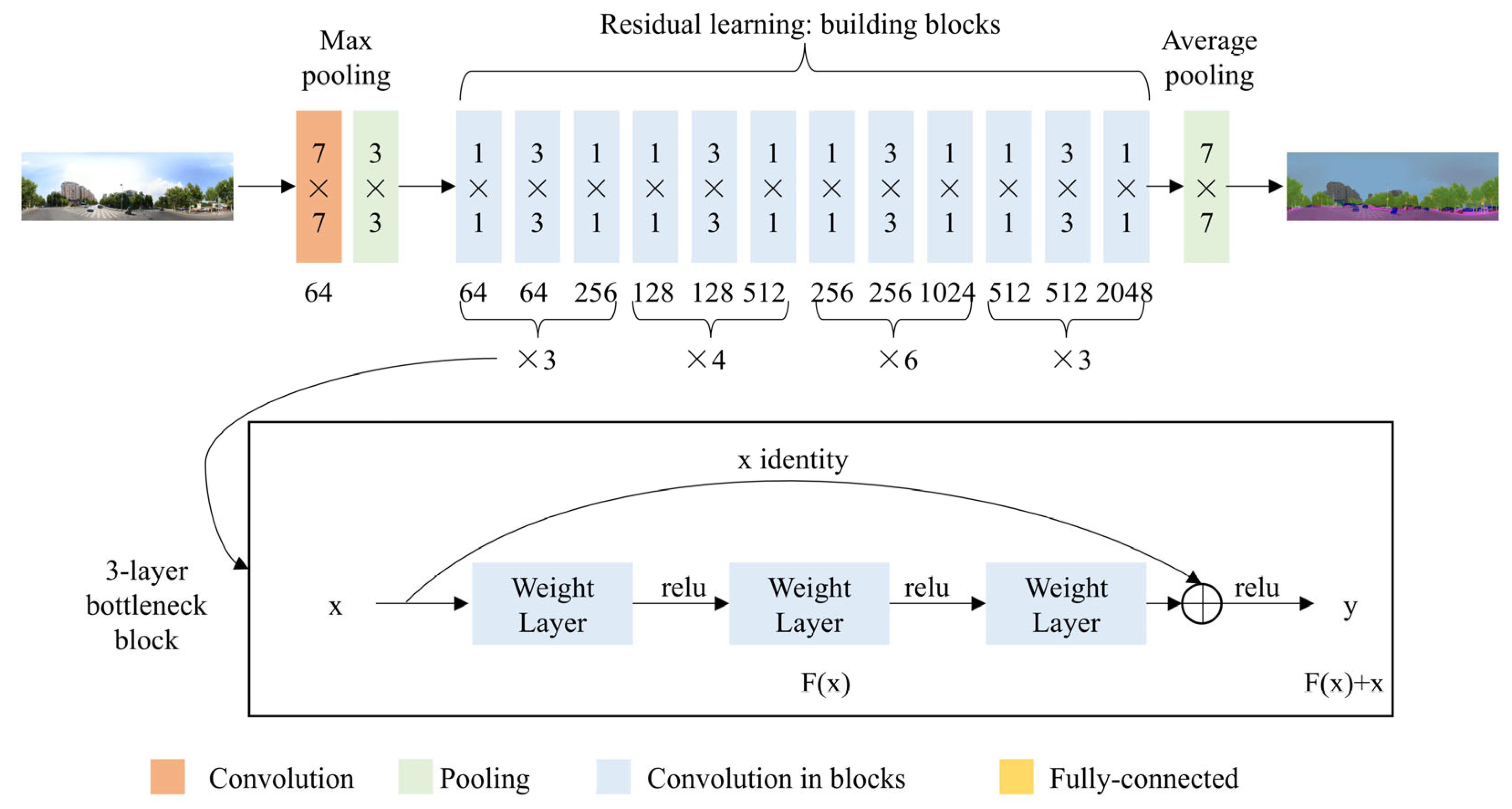
3.2. Perceptions of Urban Vitality Using ResNet50

ResNet50 is a deep residual network consisting of 50 layers in depth, which solves the problem of gradient vanishing and degradation in deep network training by introducing residual blocks, each of which passes the input features directly through a Shortcut Connection to reduce feature loss and improve training efficiency, as shown in Figure 4 [40]. ResNet50 has excellent performance in tasks such as image classification and feature extraction, and is a classical model for computer vision tasks.
Firstly, pretraining weights are initialized using ResNet50 to speed up training convergence and exploit generic features. Second, the last fully connected layer of ResNet50 is replaced with an output layer adapted to the Place Pulse 2.0 data sensing task. Then, ResNet50 is trained using the dataset to optimize the perceptual prediction capability of the model, and the model performance is evaluated with the training and validation sets to adjust the hyperparameters (e.g., learning rate and batch size). Finally, the trained ResNet50 model is migrated to the Beijing fifth ring road dataset, and the model is used to batch predict the street view images in the study area to generate the corresponding urban vitality perception scores.

3.3. GBDT Model

When examining the impact of environmental factors on UV, the relationship usually has complex nonlinear and multi-dimensional characteristics. For example, there may be a high degree of interaction and nonlinear correlation between variables such as NDVI, PopD, and AHP. Traditional linear models struggle to effectively capture these complex relationships, and a GBDT is ideal for analyzing such problems due to its powerful nonlinear modelling capabilities and adaptability to high-dimensional data [41]. GBDT is not only able to handle nonlinear relationships between multiple variables, but also quantify the contribution of each environmental variable to UV through feature importance analysis.
GBDT is an integrated learning algorithm that builds a strong regressor by combining several weak regressors. The core idea of GBDT is to iteratively train a decision tree (CART), where each CART tries to correct the errors of the previous CART, a process that is viewed as optimizing the loss function in a gradient descent process. Specifically, for the m-th base classifier, the objective minimization function is as follows:
L y , F x = ( y F ( x ) ) 2
where y is the actual value; and F x is the model prediction. The GBDT model is optimized by minimizing this objective function.
At each iteration, the residuals are calculated:
r m x i = y i F m 1 ( x i )
The residuals are then used as new labels to train the m -th base classifiers, whereby each new base regressor complements all previous base regressors. GBDT can be trained with both continuous and discrete feature data, and automatically selects features during training, and adjusts the parameters to control the complexity and bias–variance balance of the model.
As a data-driven model, GBDT can capture the nonlinear relationship between urban vitality and environmental factors by iteratively training a CART model to fit the residuals.

3.4. Shapley Additive Explanations Model

When analyzing the nonlinear effects of environmental factors on UV, we not only need to capture the complexity of the relationships, but we also need to be able to explain how each environmental variable affects the final outcome [34]. SHAP is a model interpretation method that provides a transparent, systematic explanation of predicted outcomes, and can help us understand the specific contribution of environmental variables to UV [42]. SHAP values not only reveal nonlinear interactions between characteristics, but also provide decision-makers with a more explanatory analysis that clarifies which environmental factors have a significant impact on the enhancement of UV. The Shapley value is the contribution of the feature variables to the predicted output of the model and is defined as follows:
P = S { x 1 , , x P } { x P } S ! n S 1 ! P ! ( f S x P f ( S ) )
In Formula (4), P is the Shapley value of feature p ; S is the subset of feature variables merged into the model; x P is the vector of values of feature p ; P is the number of input features; f ( S ) is the predicted value output of the feature values in the set S ; and f ( x ) is a linear function of the Shapley values of the feature variables, which can be expressed as follows:
f x = 0 + P = 1 P P Z i
In Formula (4), f ( x ) is the predicted output; 0 is the expected value of the prediction; and Z i denotes a binary feature, with Z i = 1 denoting a feature that is present and Z i = 0 denoting a feature that is absent. Among them, features with larger absolute Shapley values indicate their greater contribution to the prediction.
The SHAP value allows us to quantify the specific contribution of each environmental factor to UV. In addition, SHAP values provide a more actionable explanation for urban planning and decision-making. By analyzing SHAP values, policy-makers are able to identify which environmental factors are key drivers of UV, and thus formulate more targeted policies to optimize urban spatial structures and resource allocation.

4. Result

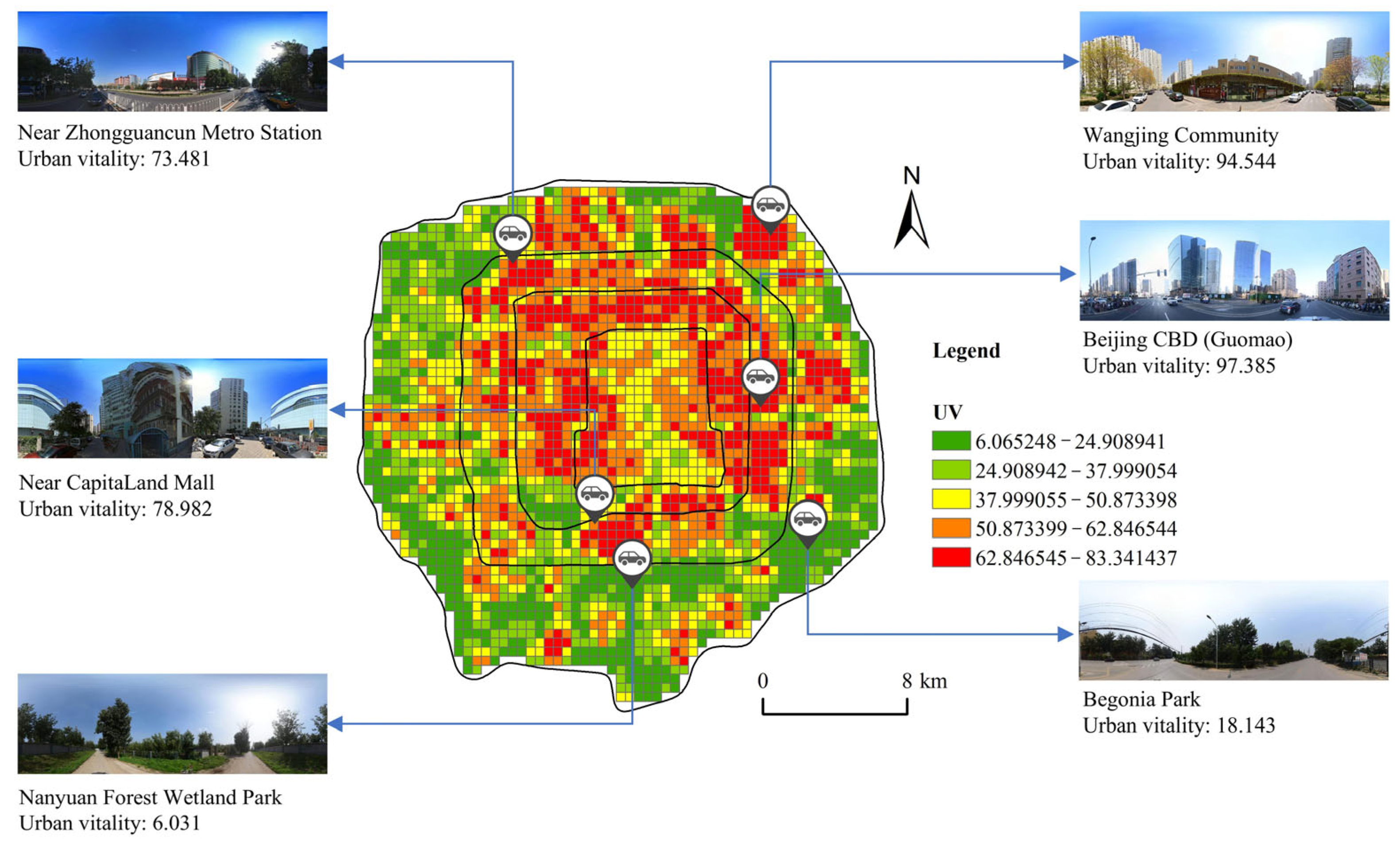
4.1. Spatial Autocorrelation Analysis of Urban Vitality

Figure 5 illustrates the spatial distribution of urban vitality in the study area surrounded by Beijing’s fifth ring road and the urban vitality values of the six demonstration sites, which show a clear radial gradient. Urban vitality forms a high-value concentric belt around the historic core, gradually declining toward the periphery. This pattern is consistent with previous studies indicating central urban areas typically exhibit higher vitality due to the concentration of economic, cultural, and transportation resources [43].
Specifically, the central high-vitality zone (UV values 50.87–83.34), shown in dark orange and red, includes areas such as Guomao (CBD), Zhongguancun, and Financial Street. These districts are characterized by intensive economic activities, dense public transport networks, high building density, and vibrant street life—all positively correlated with vitality, as shown in Section 4.4 (e.g., high AHP and PR values). This reflects the agglomeration effect of urban functions. The intermediate zone (UV 24.91–50.87), depicted in yellow and light orange, includes historic neighborhoods, like the regional commercial centers Wangjing and Wudaokou. These areas maintain moderate vitality due to mixed land use and active pedestrian environments, though are slightly constrained by limited space or aging infrastructure [44]. Peripheral areas (UV 6.06–24.91), shown in green, such as Nanyuan Forest Wetland Park and Begonia Park, have relatively low urban vitality [45]. These zones often consist of suburban ecological spaces and low-density residential areas, aligning with findings in Section 4.4 where DG and NDVI exert negative effects at certain thresholds [46]. This suggests that excessive greening or sparse development might reduce population density and pedestrian flow, thereby lowering vitality.
Numerous studies have made extensive use of local Moran’s I to identify geographical autocorrelation in the data; the Z-score evaluates spatial clustering, while the p-value indicates statistical significance. In the realm of spatial analysis, these measures have proven to be quite useful. As can be seen from Figure 6a, the ArcGIS (Version 10.8)/GeoDa (Version 1.14.0) software was used to perform a spatial autocorrelation analysis of urban vitality within the research area. The Moran’s I value for urban vitality was 0.709 with a p-value of 0.001 (less than 0.05), passing the significance test at the 5% level under a spatial weight matrix based on geographic distance, as seen in Figure 6b. This suggests that the urban vitality distribution in the investigated area has a substantial global spatial clustering trend. Furthermore, the geographical clustering was further confirmed by the Z-score beyond the crucial value of 1.96. A GBDT model was constructed by optimizing hyperparameters using cross-validation, which also provided high-precision data support for investigating the threshold effects and nonlinear interactions between urban vitality and environmental components.

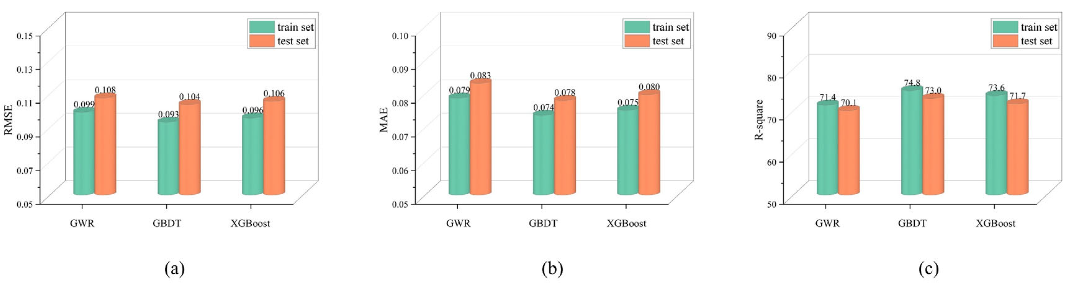
4.2. Model Comparison

In this study, the grid search method is used to optimize the hyperparameters of the GBDT model and improve the prediction accuracy. The method determines the optimal parameter combinations by systematically traversing the preset parameter space. The model in this paper has max_depth = 7, n_estimators = 1000, and learning rate = 0.01. In Figure 7, the GBDT model has the best fit, with a coefficient of determination (R2) of 0.748.
Figure 7 compares the performance of GWR, XGBoost and GBDT models based on RMSE, MAE, and R2 metrics on the training and test datasets. The results show that the GBDT model outperforms the other two models in all evaluation metrics. Specifically, GBDT has the lowest RMSE (0.093 for the training set and 0.104 for the test set) and MAE (0.074 for the training set and 0.078 for the test set), and the highest R2 values (74.8% for the training set and 73.0% for the test set). These findings highlight the GBDT model’s superior ability to capture complex nonlinear relationships.

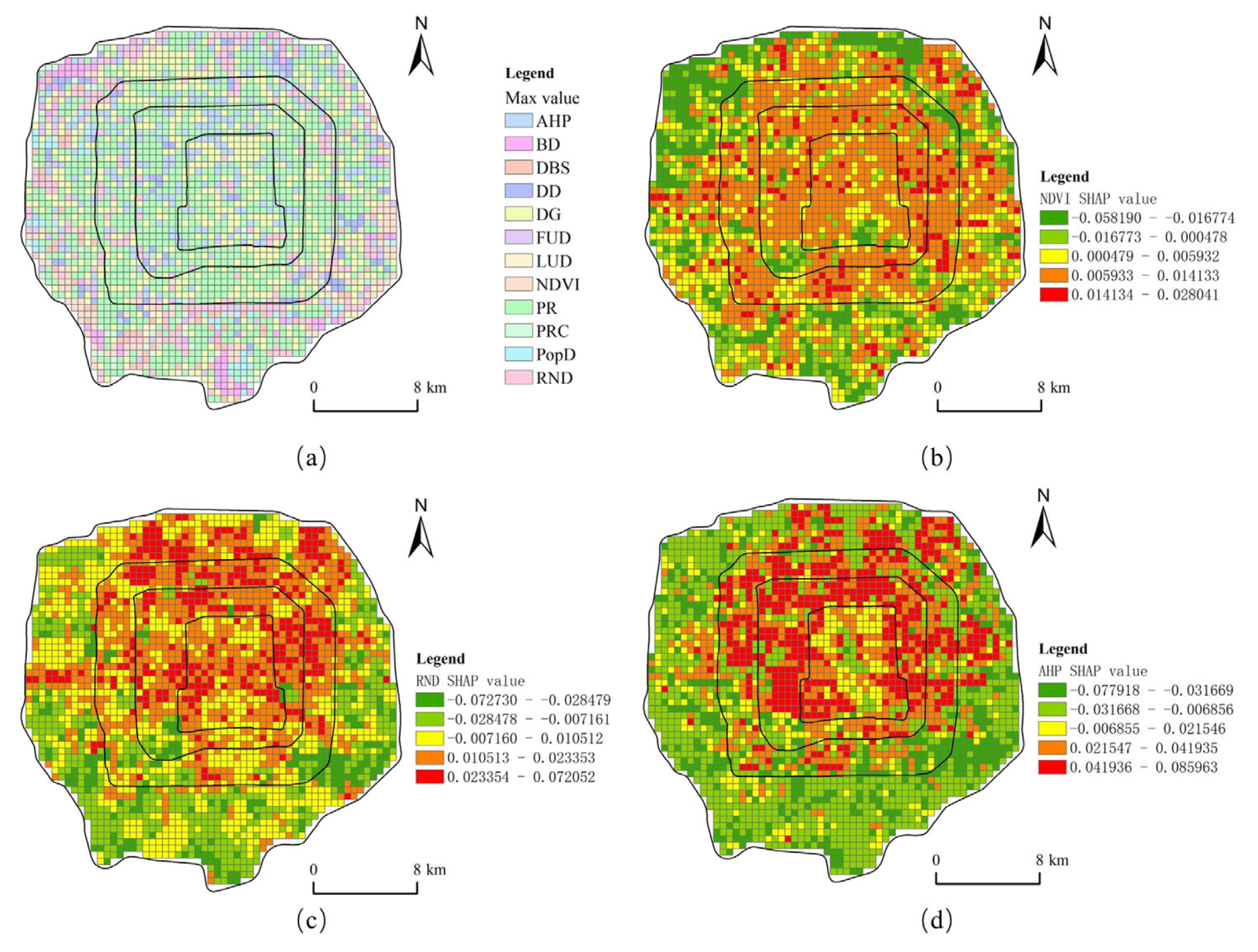
4.3. Relative Importance of Variables

As shown in Figure 8, the RI of each variable is assessed to quantify its influence. PR and DG have the largest global RI in Figure 8a, suggesting that they have a major influence on the model’s predictions. PR evaluates building density and emphasizes its crucial impact on urban life by reflecting the ratio of building area to land area. DG represents the proximity of a grid to the nearest green space, such as a park, and underscores the role of natural environments in enhancing urban functionality. Following these, AHP and RND demonstrate substantial importance, emphasizing the significance of economic and transportation variables in the model. Meanwhile, NDVI highlights the relevance of vegetation coverage to predictions.
Figure 8b illustrates the distribution of SHAP values for PR and AHP, showing wide ranges where higher values significantly increase the model’s predicted output, while lower values reduce it. The SHAP values for DG reveal that lower DG values positively influence the model output, while higher DG values negatively affect predictions, emphasizing the importance of green space accessibility for enhancing vitality. Similarly, high NDVI values positively impact the model output, aligning with the ecological and psychological benefits of green spaces [47]. Both RND and FUD show positive effects, indicating that a well-developed transportation network and functional diversity are key drivers of urban vitality [21]. Integrating insights from Figure 8a,b, PR, DG, AHP, and RND emerge as the critical variables influencing the model’s predictions. These findings reflect the combined effects of spatial utilization, environmental accessibility, economic conditions, and transportation layout.
Figure 9a shows the impact factors with the largest SHAP values for each grid. Figure 9 shows that PR, DG, and AHP have high RIs and are highly influential across the impact factors. Interestingly, variables of lower importance, such as DBS and NDVI, also show significant performance at the local scale in Figure 8. We also visualize the spatial distribution of the SHAP values of some important variables in each GVI (Figure 9b,c), such as NDVI, RND, and AHP. RND mainly positively affects the areas along the roads within the fifth ring road, which are usually conveniently accessible to attract more people to the vicinity of the intersections for commercial, social, or recreational activities, and this clustering of people directly enhances the city’s vitality [48]. Higher property prices help to optimize land-use, transport, and environmental factors to enhance urban vitality and sustainability within the third ring road.

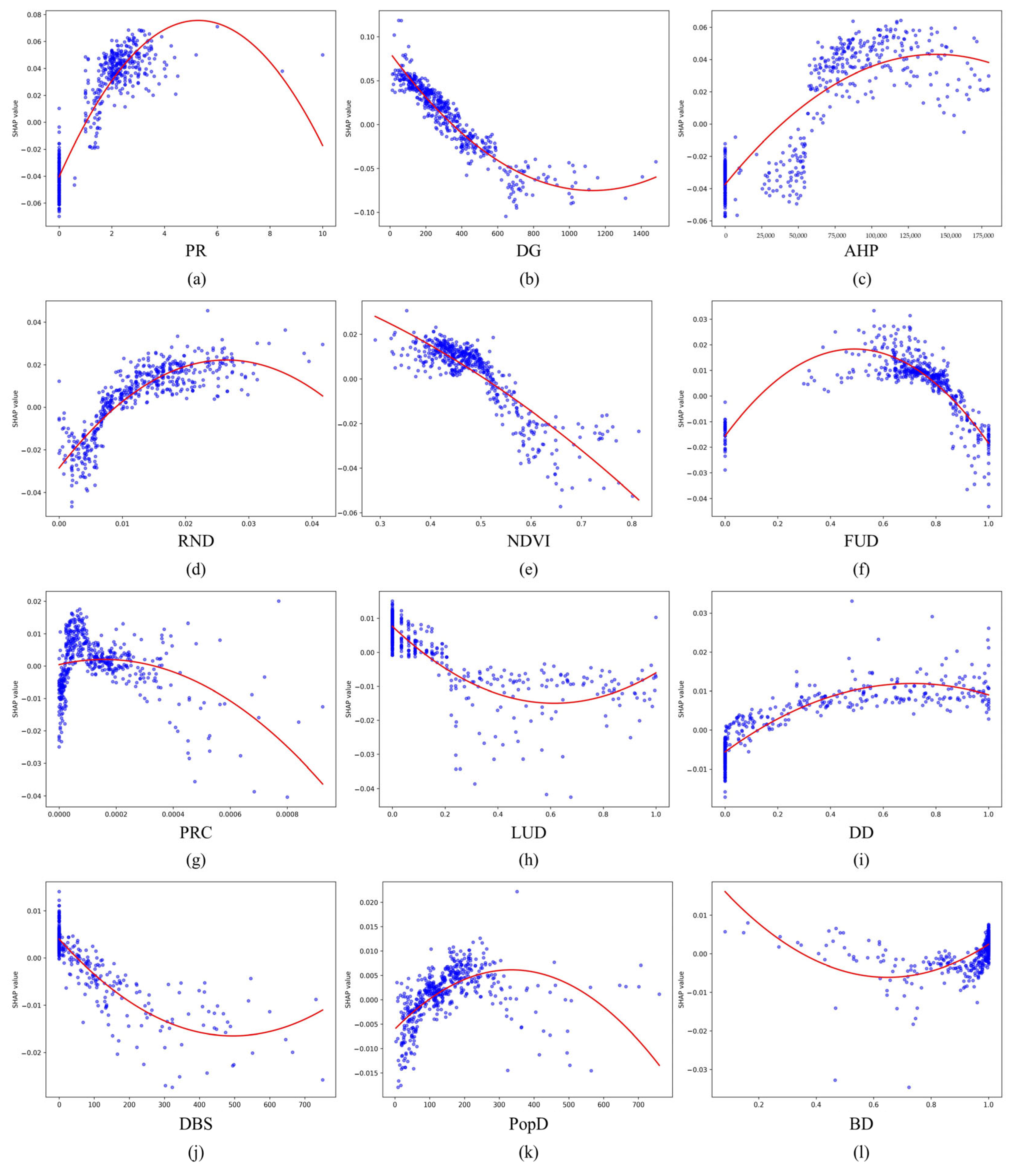
4.4. Nonlinear Association Analysis

Urban vitality and the affecting elements have nonlinear correlations, according to the investigation. This section visualizes the SHAP values of each variable in the urban vitality model using LDPs to provide a clear explanation of these relationships. Based on LDPs, threshold effects and nonlinear patterns are investigated. As shown in Figure 10, LDPs were employed to visualize the SHAP values of variables. Through LDP analysis, we examined the nonlinear relationships and identified threshold effects. When PopD is below 50, the local effect is positive, indicating that moderate population density can enhance urban vitality [43]. However, when PopD exceeds 50, the local effect turns negative, suggesting that excessive population density may impose resource pressures that suppress urban vitality. For BD, the local effect becomes negative [49] when it exceeds approximately 0.7, implying that increased building density restricts green space distribution and negatively impacts urban vitality. A similar trend is observed for PR, where higher values of PR significantly reduce urban vitality, highlighting how high plot ratios compress urban green spaces. When RND is within the range of 0.01 to 0.03, the local effect is positive, indicating that appropriate road density alleviates urban vitality deficiencies. However, as RND increases further, the local effect becomes negative, suggesting that excessive road density may lead to traffic congestion or reduce open spaces, thereby diminishing urban vitality. A similar pattern is observed for PRC, where overly dense intersections negatively affect urban vitality. For DG, the local effect is positive when DG is less than 200, demonstrating that areas closer to green spaces typically exhibit higher urban vitality. However, when DG exceeds 200, the local effect turns negative, indicating that being far from green spaces significantly reduces urban vitality [50]. Similarly, PD is positively correlated with urban vitality, indicating that increasing park density helps mitigate urban vitality deficiencies. When DD is below 0.2, the local effect is positive, suggesting that a moderate distribution of commercial facilities enhances urban vitality. However, when DD exceeds 0.2, the local effect becomes negative, as excessive commercial density can lead to overcrowding or environmental issues, suppressing urban vitality. For DBS, the local effect becomes positive when DBS exceeds 500, indicating that areas farther from transportation hubs may have higher urban vitality, possibly due to reduced noise or congestion from transit activities. When FUD exceeds 0.5, the local effect shifts from negative to positive, demonstrating that areas with higher functional diversity generally exhibit greater urban vitality [50]. Additionally, AHP is positively associated with urban vitality, suggesting that high housing price areas tend to have greater urban vitality [51], possibly due to an emphasis on environment and greenery in these areas. The positive correlation between building age and urban vitality highlights that redevelopment and optimization of older neighborhoods may contribute to improved urban vitality.
In conclusion, the influencing factors exhibit significant nonlinear relationships with urban vitality, and the threshold effects and interactions among variables play crucial roles in the spatial distribution of urban vitality.

5. Discussion

5.1. Overall Evaluation of the Experiment

This study investigates the distribution of urban vitality in Beijing, focusing on areas within the fifth ring road, and uses advanced analytical techniques to understand the spatial correlations and build a model of urban vitality. The distribution of vitality values is in the shape of concentric circles, with higher values in the urban core and values gradually decreasing towards the periphery. This spatial pattern is consistent with the findings of Xiao et al. [51], who observed similar concentric vitality structures in high-density Chinese cities, reflecting the urban core–periphery dynamic driven by access to services and infrastructure.
In addition, this study proposes a unique framework to explore the nonlinear association between environmental factors and urban vitality using an interpretable GBDT model. Unlike previous work based on linear assumptions and regression models, our framework establishes an interpretable model that addresses the complexity of the nonlinear relationships among factors. Previous studies, such as Zhang et al. [43], have relied on Geographically Weighted Regression (GWR) to model spatially varying impacts, but failed to capture threshold effects and complex non-monotonic relationships, which are effectively handled in our model. At the same time, we utilize a local explanatory model to comprehensively explain the nonlinear associations between the factors, thus overcoming the limitations of previous regression models that are unexplainable. The GBDT model outperforms the GWR and XGBoost in predicting urban vitality, as evidenced by its higher R2 and lower RMSE and MAE. Our framework highlights the nonlinear characteristics among the factors, providing valuable insights into which regions may need more attention.

5.2. Influence of Built Environment Factors on Urban Vitality

This study shows that NDVI and urban vitality in the urban areas of Beijing show a significant negative correlation. Data analysis showed that areas with high vegetation cover, such as large parks and densely green residential areas, tended to exhibit lower levels of urban vitality. This finding is in line with previous findings by Jiang et al., that over-concentrated green space may reduce the area’s population aggregation and activity frequency [52]. Similarly, Li et al. [53] noted that excessive urban greening in peripheral zones might reduce land-use efficiency and weaken functional integration, supporting our interpretation of a spatial trade-off. This association reflects a potential spatial trade-off between urban greening and urban vitality. Through statistical analysis, NDVI is the fifth most influential factor of urban vitality. This suggests that urban vitality is mainly dominated by other urban factors, such as the distribution of commercial facilities and transport accessibility. Therefore, when optimizing the urban spatial layout, it is necessary to balance the scale of the allocation of green space and other urban functions to establish a more comprehensive evaluation system of urban vitality.
This study investigates the relationship between urban vitality and multiple built environment factors in Beijing, revealing significant nonlinear characteristics in their impacts. PR exerts a notable negative influence on urban vitality. This is consistent with the results of Chen et al. [54], who found that beyond specific density thresholds, the benefits of compact development reverse due to traffic congestion and reduced livability. As PR increases, urban vitality gradually declines, primarily because high plot ratios compress green space, intensify regional congestion, and deteriorate microclimate conditions. Moreover, elevated PR often leads to land-use homogenization, restricting the diversity of social and economic activities, and thereby hindering urban vitality enhancement. Similarly, DG significantly affects urban vitality, demonstrating a nonlinear threshold effect. Low DG values, indicating better green space accessibility, significantly enhance urban vitality. Other critical variables, such as the NDVI and RND, also contribute substantially to urban vitality, reflecting the integrated impacts of vegetation coverage, economic conditions, and transportation layouts on urban vitality.
This study further uncovers the complex threshold effects of built environment variables. PopD and BD positively influence urban vitality within moderate ranges but exhibit negative impacts once exceeding certain critical thresholds, highlighting the suppressive effects of overdevelopment on urban vitality. Similarly, FUD shows a transition from negative to positive effects on urban vitality, emphasizing the importance of multifunctional spatial planning in enhancing urban vitality. DD is another important factor. A moderate level of commercial concentration can stimulate economic activity, promote social interaction, and enhance regional vitality. However, over-intensive commercial development often comes at the expense of green space and public space, which not only harms the ecological environment, but also reduces the quality of life of the residents and restricts the sustainable development of the city. By employing the SHAP interpretive framework, this study systematically reveals the spatial distribution of urban vitality in Beijing and its nonlinear relationships with built environment factors. The findings provide scientific evidence for urban planning and resource allocation, offering insights into optimizing green resources, improving transportation layouts, and balancing built environment and economic factors to enhance urban vitality.

5.3. Influence of Socioeconomic Factors on Urban Vitality

The urban vitality is influenced by a number of key elements of the built environment. Research has shown that AHP is the most decisive factor. High housing prices in economically developed regions tend to reflect high quality amenities and a wealth of socioeconomic activities, characteristics that contribute to regional vitality [55].
Therefore, urban planning should focus on balancing these key elements, preventing social segregation by controlling the level of property prices, while maintaining a moderate commercial density and ensuring a reasonable allocation of green space and public space. This balanced development strategy will help to promote social interaction, enhance the well-being of residents, and achieve sustained growth in urban vitality.

5.4. Limitations and Future Research Directions

Despite the strengths of this study in introducing a perceptual, interpretable, and data-driven framework for urban vitality assessment, several limitations should be acknowledged. First, the use of street-level imagery from the Place Pulse 2.0 dataset, while valuable in capturing visual perception, may not fully represent real-time urban dynamics, especially in rapidly changing environments. Additionally, although SHAP values provide interpretability, their global explanations may overlook subtle local patterns or interactions between variables. In addition, this study employed a uniform 500 m × 500 m grid to aggregate and analyze multi-source spatial data. Specifically, the use of fixed grids may disrupt the continuity of physical spaces, potentially splitting functionally cohesive entities such as schools, residential compounds, or commercial zones. Moreover, grids do not inherently account for the actual spatial interactions or built environment connectivity between adjacent units. At last, indicators such as building height, form diversity, pedestrian infrastructure, or street canyon geometry were not included due to data availability constraints.
Future research could address these limitations in several ways. First, integrating multi-source real-time data—such as mobility traces, urban sensors, and social media feeds—would enrich the measurement of urban vitality and better reflect its temporal evolution. Second, adopting multimodal models that combine imagery with textual and spatial datasets may provide a more holistic understanding of urban life. Third, future research may consider adopting spatial units defined by functional or morphological boundaries, such as road-enclosed parcels or administrative blocks, which better reflect the spatial structure of urban environments and enable a more nuanced understanding of localized vitality patterns. Additionally, advances in interpretable deep learning, such as attention-based spatial–temporal graph neural networks, could be leveraged to capture complex dependencies while maintaining transparency. Cross-city transfer learning techniques could also be employed to test model robustness and generalizability across different urban contexts. Ultimately, future research should aim for more comprehensive, dynamic, and inclusive assessments of urban vitality, combining human-centered perspectives with scalable machine learning tools.

6. Conclusions

This study integrates multi-source urban big data to develop a spatial machine learning framework aimed at analyzing the complex relationships between environmental variables and urban vitality. The GBDT model was utilized to handle nonlinear relationships, and the SHAP framework was utilized to offer a thorough and in-depth analysis of the findings. The geographical impacts and nonlinear connections of many environmental variables on urban vitality were investigated in detail under this paradigm. The results show the following:
(1)
Urban vitality within Beijing’s fifth ring road exhibits significant spatial clustering and positive correlations, characterized by marked spatial heterogeneity with aggregated distribution in both hot-spot and cold-spot areas.
(2)
The optimized GBDT model, tuned via grid search, outperforms GWR and XGBoost by achieving the best overall prediction accuracy, effectively capturing complex nonlinear relationships.
(3)
Among all the environmental variables, PR demonstrates the strongest positive influence on urban vitality, whereas DG exhibits the most significant negative correlation with urban vitality.
(4)
The study reveals notable nonlinear and threshold effects of DG, the built environment, and socioeconomic conditions on urban vitality.
These nonlinearities and thresholds provide valuable quantitative tools for urban planning, enabling the rational allocation of urban resources, optimization of greening strategies, enhancement of low-vitality areas, and prevention of resource wastage. Future applications may include comparative studies across cities (e.g., comparing Beijing with international cities such as Tokyo, London, or São Paulo), longitudinal analyses to assess vitality change over time, or integration into decision-support systems for real-time urban planning. Overall, this research advances both the theory and practice of urban vitality analysis, providing replicable tools for sustainable, human-centered urban development worldwide.

Author Contributions

Conceptualization, D.L.; methodology, J.W.; software, D.L.; validation, X.X.; formal analysis, D.L.; investigation, D.L.; resources, D.L.; data curation, D.L.; writing—original draft preparation, D.L.; writing—review and editing, D.L.; visualization, D.L.; supervision, D.L.; project ad-ministration, H.H.; funding acquisition, D.L. All authors have read and agreed to the published version of the manuscript.

Funding

This research was funded by the National Natural Science Foundation of China (Grant No. 42374024 and No. 42274029), the Beijing Nova Program (Grant No. 20230484270), and the Doctor Graduate Scientific Research Ability Improvement Project of Beijing University of Civil Engineering and Architecture (DG2024033, DG2024034 and DG2025034).

Institutional Review Board Statement

Not applicable.

Informed Consent Statement

Not applicable.

Data Availability Statement

All data generated or analyzed during this study are included in this article.

Conflicts of Interest

The authors declare no conflict of interest.

References

  1. Liu, H.; Gou, P.; Xiong, J. Vital triangle: A new concept to evaluate urban vitality. Comput. Environ. Urban Syst. 2022, 98, 101886. [Google Scholar] [CrossRef]
  2. Jiang, Y.; Han, Y.; Liu, M.; Ye, Y. Street vitality and built environment features: A data-informed approach from fourteen Chinese cities. Sustain. Cities Soc. 2022, 79, 103724. [Google Scholar] [CrossRef]
  3. Yue, W.; Chen, Y.; Thy, P.T.M.; Fan, P.; Liu, Y.; Zhang, W. Identifying urban vitality in metropolitan areas of developing countries from a comparative perspective: Ho Chi Minh City versus Shanghai. Sustain. Cities Soc. 2021, 65, 102609. [Google Scholar] [CrossRef]
  4. Dogan, O.; Lee, S. Jane Jacobs’s urban vitality focusing on three-facet criteria and its confluence with urban physical complexity. Cities 2024, 155, 105446. [Google Scholar] [CrossRef]
  5. Glaeser, E. Cities, Productivity, and Quality of Life. Science 2011, 333, 592–594. [Google Scholar] [CrossRef]
  6. Wu, C.; Ye, X.; Ren, F.; Du, Q. Check-in behaviour and spatio-temporal vibrancy: An exploratory analysis in Shenzhen, China. Cities 2018, 77, 104–116. [Google Scholar] [CrossRef]
  7. Yue, Y.; Zhuang, Y.; Yeh, A.G.O.; Xie, J.Y.; Ma, C.L.; Li, Q.Q. Measurements of POI-based mixed use and their relationships with neighbourhood vibrancy. Int. J. Geogr. Inf. Sci. 2017, 31, 658–675. [Google Scholar] [CrossRef]
  8. Huang, B.; Zhou, Y.; Li, Z.; Song, Y.; Cai, J.; Tu, W. Evaluating and characterizing urban vibrancy using spatial big data: Shanghai as a case study. Environ. Plan. B Urban Anal. City Sci. 2019, 47, 1543–1559. [Google Scholar] [CrossRef]
  9. Delclòs-Alió, X.; Miralles-Guasch, C. Looking at Barcelona through Jane Jacobs’s eyes: Mapping the basic conditions for urban vitality in a Mediterranean conurbation. Land Use Policy 2018, 75, 505–517. [Google Scholar] [CrossRef]
  10. Wu, J.; Ta, N.; Song, Y.; Lin, J.; Chai, Y. Urban form breeds neighborhood vibrancy: A case study using a GPS-based activity survey in suburban Beijing. Cities 2018, 74, 100–108. [Google Scholar] [CrossRef]
  11. Jin, X.; Long, Y.; Sun, W.; Lu, Y.; Yang, X.; Tang, J. Evaluating cities’ vitality and identifying ghost cities in China with emerging geographical data. Cities 2017, 63, 98–109. [Google Scholar] [CrossRef]
  12. Wang, B.; Zhen, F.; Wei, Z.; Guo, S.; Chen, T. A theoretical framework and methodology for urban activity spatial structure in e-society: Empirical evidence for Nanjing City, China. Chin. Geogr. Sci. 2015, 25, 672–683. [Google Scholar] [CrossRef]
  13. Long, Y.; Huang, C.C. Does block size matter? The impact of urban design on economic vitality for Chinese cities. Environ. Plan. B Urban Anal. City Sci. 2017, 46, 406–422. [Google Scholar] [CrossRef]
  14. Ye, Y.; Li, D.; Liu, X. How block density and typology affect urban vitality: An exploratory analysis in Shenzhen, China. Urban Geogr. 2018, 39, 631–652. [Google Scholar] [CrossRef]
  15. Xia, C.; Yeh, A.G.-O.; Zhang, A. Analyzing spatial relationships between urban land use intensity and urban vitality at street block level: A case study of five Chinese megacities. Landsc. Urban Plan. 2020, 193, 103669. [Google Scholar] [CrossRef]
  16. Kim, Y.-L. Seoul’s Wi-Fi hotspots: Wi-Fi access points as an indicator of urban vitality. Comput. Environ. Urban Syst. 2018, 72, 13–24. [Google Scholar] [CrossRef]
  17. Xiao, L.; Lo, S.; Zhou, J.; Liu, J.; Yang, L. Predicting vibrancy of metro station areas considering spatial relationships through graph convolutional neural networks. Case Shenzhen China 2021, 48, 2363–2384. [Google Scholar] [CrossRef]
  18. Yang, J.; Cao, J.; Zhou, Y. Elaborating non-linear associations and synergies of subway access and land uses with urban vitality in Shenzhen. Transp. Res. Part A Policy Pract. 2021, 144, 74–88. [Google Scholar] [CrossRef]
  19. Pengjun, Z.; Jia, L.U.O.; Haoyu, H.U. Spatial match between residents’ daily life circle and public service facilities using big data analytics: A case of Beijing. Prog. Geogr. 2021, 40, 541–553. [Google Scholar] [CrossRef]
  20. Cong, W.; Zhou, J.; Lai, Y. The coordination between citywide rail transit accessibility and land-use characteristics in Shenzhen, China: An explorative analysis based on multidimensional spatial data. Sustain. Cities Soc. 2024, 113, 105691. [Google Scholar] [CrossRef]
  21. Long, Y.; Wu, Y.; Huang, L.; Aleksejeva, J.; Iossifova, D.; Dong, N.; Gasparatos, A. Assessing urban livability in Shanghai through an open source data-driven approach. NPJ Urban Sustain. 2024, 4, 7. [Google Scholar] [CrossRef]
  22. Sicong, Z.O.U.; Shanqi, Z.; Feng, Z. Measurement of community daily activity space and influencing factors of vitality based on residents’ spatiotemporal behavior: Taking Shazhou and Nanyuan streets in Nanjing as examples. Prog. Geogr. 2021, 40, 580–596. [Google Scholar] [CrossRef]
  23. Wang, B.; Lei, Y.; Xue, D.; Liu, J.; Wei, C. Elaborating Spatiotemporal Associations Between the Built Environment and Urban Vibrancy: A Case of Guangzhou City, China. Chin. Geogr. Sci. 2022, 32, 480–492. [Google Scholar] [CrossRef]
  24. Li, D.; Liu, J.; Zhao, Y. Prediction of Multi-Site PM2.5 Concentrations in Beijing Using CNN-Bi LSTM with CBAM. Atmosphere 2022, 13, 1719. [Google Scholar] [CrossRef]
  25. Li, D.; Liu, J.; Zhao, Y. Forecasting of PM2.5 Concentration in Beijing Using Hybrid Deep Learning Framework Based on Attention Mechanism. Appl. Sci. 2022, 12, 11155. [Google Scholar] [CrossRef]
  26. Li, D.; Wang, J.; Tian, D.; Chen, C.; Xiao, X.; Wang, L.; Wen, Z.; Yang, M.; Zou, G. Residual neural network with spatiotemporal attention integrated with temporal self-attention based on long short-term memory network for air pollutant concentration prediction. Atmos. Environ. 2024, 329, 120531. [Google Scholar] [CrossRef]
  27. Zhaomin, T.; Rui, A.N.; Yaolin, L.I.U. Impact of the built environment on residents’ commuting mode choices: A case study of urban village in Wuhan City. Prog. Geogr. 2021, 40, 2048–2060. [Google Scholar] [CrossRef]
  28. Liu, J.; Wang, B.; Xiao, L. Non-linear associations between built environment and active travel for working and shopping: An extreme gradient boosting approach. J. Transp. Geogr. 2021, 92, 103034. [Google Scholar] [CrossRef]
  29. Chen, C.; Wang, J.; Li, D.; Sun, X.; Zhang, J.; Yang, C.; Zhang, B. Unraveling nonlinear effects of environment features on green view index using multiple data sources and explainable machine learning. Sci. Rep. 2024, 14, 30189. [Google Scholar] [CrossRef]
  30. Jerome, H.F. Greedy function approximation: A gradient boosting machine. Ann. Stat. 2001, 29, 1189–1232. [Google Scholar] [CrossRef]
  31. Yang, W.; Li, Y.; Liu, Y.; Fan, P.; Yue, W. Environmental factors for outdoor jogging in Beijing: Insights from using explainable spatial machine learning and massive trajectory data. Landsc. Urban Plan. 2024, 243, 104969. [Google Scholar] [CrossRef]
  32. Ben Khedher, M.B.; Yun, D. An Interpretable Machine Learning-Based Hurdle Model for Zero-Inflated Road Crash Frequency Data Analysis: Real-World Assessment and Validation. Appl. Sci. 2024, 14, 10790. [Google Scholar] [CrossRef]
  33. Pasic, M.; Marinkovic, D.; Lukic, D.; Begic-Hajdarevic, D.; Zivkovic, A.; Milosevic, M.; Muhamedagic, K. Prediction and Optimization of Surface Roughness and Cutting Forces in Turning Process Using ANN, SHAP Analysis, and Hybrid MCDM Method. Appl. Sci. 2024, 14, 11386. [Google Scholar] [CrossRef]
  34. Santamato, V.; Tricase, C.; Faccilongo, N.; Iacoviello, M.; Pange, J.; Marengo, A. Machine Learning for Evaluating Hospital Mobility: An Italian Case Study. Appl. Sci. 2024, 14, 6016. [Google Scholar] [CrossRef]
  35. Plakias, S.; Kokkotis, C.; Mitrotasios, M.; Armatas, V.; Tsatalas, T.; Giakas, G.J.A.S. Identifying Key Factors for Securing a Champions League Position in French Ligue 1 Using Explainable Machine Learning Techniques. Appl. Sci. 2024, 14, 8375. [Google Scholar] [CrossRef]
  36. Dubey, A.; Naik, N.; Parikh, D.; Raskar, R.; Hidalgo, C.A. Deep Learning the City: Quantifying Urban Perception at a Global Scale. In Computer Vision—ECCV 2016: 14th European Conference, Amsterdam, The Netherlands, 11–14 October 2016, Proceedings, Part I; Springer International Publishing: Cham, Switzerland, 2016; pp. 196–212. [Google Scholar]
  37. Wei, J.; Yue, W.; Li, M.; Gao, J. Mapping human perception of urban landscape from street-view images: A deep-learning approach. Int. J. Appl. Earth Obs. Geoinf. 2022, 112, 102886. [Google Scholar] [CrossRef]
  38. Shi, J.; Miao, W.; Si, H.; Liu, T. Urban Vitality Evaluation and Spatial Correlation Research: A Case Study from Shanghai, China. Land 2021, 10, 1195. [Google Scholar] [CrossRef]
  39. Niu, S.; Hu, A.; Shen, Z.; Huang, Y.; Mou, Y. Measuring the built environment of green transit-oriented development: A factor-cluster analysis of rail station areas in Singapore. Front. Archit. Res. 2021, 10, 652–668. [Google Scholar] [CrossRef]
  40. He, K.; Zhang, X.; Ren, S.; Sun, J. Deep Residual Learning for Image Recognition. In Proceedings of the 2016 IEEE Conference on Computer Vision and Pattern Recognition (CVPR), Las Vegas, NV, USA, 27–30 June 2016; pp. 770–778. [Google Scholar]
  41. Zhang, B.; Zou, G.; Qin, D.; Ni, Q.; Mao, H.; Li, M. RCL-Learning: ResNet and convolutional long short-term memory-based spatiotemporal air pollutant concentration prediction model. Expert Syst. Appl. 2022, 207, 118017. [Google Scholar] [CrossRef]
  42. Yang, W.; Fei, J.; Li, Y.; Chen, H.; Liu, Y. Unraveling nonlinear and interaction effects of multilevel built environment features on outdoor jogging with explainable machine learning. Cities 2024, 147, 104813. [Google Scholar] [CrossRef]
  43. Chen, Y.; Yu, B.; Shu, B.; Yang, L.; Wang, R. Exploring the spatiotemporal patterns and correlates of urban vitality: Temporal and spatial heterogeneity. Sustain. Cities Soc. 2023, 91, 104440. [Google Scholar] [CrossRef]
  44. Bao, Z.; Ou, Y.; Chen, S.; Wang, T. Land Use Impacts on Traffic Congestion Patterns: A Tale of a Northwestern Chinese City. Land 2022, 11, 2295. [Google Scholar] [CrossRef]
  45. Li, M.; Pan, J. Assessment of Influence Mechanisms of Built Environment on Street Vitality Using Multisource Spatial Data: A Case Study in Qingdao, China. Sustainability 2023, 15, 1518. [Google Scholar] [CrossRef]
  46. Ding, J.; Luo, L.; Shen, X.; Xu, Y. Influence of built environment and user experience on the waterfront vitality of historical urban areas: A case study of the Qinhuai River in Nanjing, China. Front. Archit. Res. 2023, 12, 820–836. [Google Scholar] [CrossRef]
  47. Xie, Y.; Zhang, J.; Li, Y.; Zhu, Z.; Deng, J.; Li, Z. Integrating Multi-Source Urban Data with Interpretable Machine Learning for Uncovering the Multidimensional Drivers of Urban Vitality. Land 2024, 13, 2028. [Google Scholar] [CrossRef]
  48. Zhang, P.; Zhang, T.; Fukuda, H.; Ma, M. Evidence of Multi-Source Data Fusion on the Relationship between the Specific Urban Built Environment and Urban Vitality in Shenzhen. Sustainability 2023, 15, 6869. [Google Scholar] [CrossRef]
  49. Honghu, S.U.N.; Yupei, J. Spatial heterogeneity of the impact of built environment on urban vitality: A case study of the central urban area of Nanjing. Geogr. Res. 2024, 43, 1700–1714. [Google Scholar] [CrossRef]
  50. Xu, D.; Zhou, D.; Wang, Y.; Meng, X.; Gu, Z.; Yang, Y. Temporal and spatial heterogeneity research of urban anthropogenic heat emissions based on multi-source spatial big data fusion for Xi’an, China. Energy Build. 2021, 240, 110884. [Google Scholar] [CrossRef]
  51. Xiao, Z.; Li, C.; Pan, S.; Wei, G.; Tian, M.; Hu, R. Exploring the Spatial Impact of Multisource Data on Urban Vitality: A Causal Machine Learning Method. Wirel. Commun. Mob. Comput. 2022, 2022, 5263376. [Google Scholar] [CrossRef]
  52. Jiang, B.; Larsen, L.; Deal, B.; Sullivan, W.C. A dose–response curve describing the relationship between tree cover density and landscape preference. Landsc. Urban Plan. 2015, 139, 16–25. [Google Scholar] [CrossRef]
  53. Li, G.; Cao, Y.; Fang, C.; Sun, S.; Qi, W.; Wang, Z.; He, S.; Yang, Z. Global urban greening and its implication for urban heat mitigation. Proc. Natl. Acad. Sci. USA 2025, 122, e2417179122. [Google Scholar] [CrossRef] [PubMed]
  54. Chen, H.; Jia, B.; Lau, S.S.Y. Sustainable urban form for Chinese compact cities: Challenges of a rapid urbanized economy. Habitat Int. 2008, 32, 28–40. [Google Scholar] [CrossRef]
  55. Ünalan, G.; Çamalan, Ö.; Yılmaz, H.H. The Impact of Increases in Housing Prices on Income Inequality: A Perspective on Sustainable Urban Development. Sustainability 2025, 17, 4024. [Google Scholar] [CrossRef]
Figure 1. Study area of Beijing.
Sustainability 17 04926 g001
Figure 2. Visual presentation of the selected variables. (a) NDVI; (b) LUD; (c) PRC; (d) BD.
Sustainability 17 04926 g002
Figure 3. Study design and workflow.
Sustainability 17 04926 g003
Figure 4. ResNet50 model structure and layer configuration.
Sustainability 17 04926 g004
Figure 5. Spatial distribution of urban vitality and demonstration sites.
Sustainability 17 04926 g005
Figure 6. Autocorrelation analysis plot. (a) Spatial distribution of the Moran Index; (b) Scatterplot of the Moran Index.
Sustainability 17 04926 g006
Figure 7. Model performance comparison. (a) RMSE; (b) MAE; (c) R2.
Sustainability 17 04926 g007
Figure 8. Relative importance of predictors and a SHAP summary plot. (a) Mean (|SHAP value|); (b) SHAP value.
Sustainability 17 04926 g008
Figure 9. SHAP feature importance visualization of partial variables. (a) The largest SHAP values for each grid; (b) SHAP value of NDVI; (c) SHAP value of RND; (d) SHAP value of AHP.
Sustainability 17 04926 g009
Figure 10. SHAP dependence plots for all variables. (a) PR; (b) DG; (c) AHP; (d) RND; (e) NDVI; (f) FUD; (g) PRC; (h) LUD; (i) DD; (j) DBS; (k) PopD; (l) BD.
Sustainability 17 04926 g010
Table 1. Descriptive statistics of the variables.
VariablesAbbreviationFormulaDescriptions
Urban vitality indexUV Grid’s average urban vitality value
Built environment data
Normalized difference vegetation indexNDVI [38]-Grid’s average NDVI value
Population densityPopD N a S S   is   the   grid s   area ,   and   N a is the total number of users.
Building densityBD S a S The   building   footprint s   overall   area   in   the   grid   is   denoted   by   S a .
Road network densityRND L a S The   road   network s   overall   mileage   inside   the   grid   is   denoted   by   L a .
Land-use diversityLUD i = 1 n P i l n   ( P i ) l n   ( n ) n   is   the   number   of   total   land - use   categories ,   and   P i   is   the   proportion   of   land - use   type   i in the region of the grid to which it belongs.
Functional utilization diversityFUD i = 1 m P j l n   ( P j ) l n   ( m ) m   is   the   total   number   of   categories   in   the   functional   area ,   and   P j is the percentage of category j functional area types in the region of the grid to which they belong.
Point of road connectivityPRC N b S The   number   of   road   nodes   in   the   grid   is   denoted   by   N b .
Plot ratioPR S b S u The gross floor area above ground of each building in the grid is denoted by S b .
The distance to the closest metro station and bus stopDBS-The separation between the grid halfway and the nearest bus stop and subway station.
The distance to the closest parkDG-The distance between the middle of the grid and the nearest park.
Business densityDD S c S S c is the total area occupied by financial facilities in the grid.
Socioeconomic data
Average house priceAHP-Average house price in the grid.
Disclaimer/Publisher’s Note: The statements, opinions and data contained in all publications are solely those of the individual author(s) and contributor(s) and not of MDPI and/or the editor(s). MDPI and/or the editor(s) disclaim responsibility for any injury to people or property resulting from any ideas, methods, instructions or products referred to in the content.

