Article

Assessment of Urban Green Space Equity in Beijing’s Central Urban Villages: A Remote Sensing Perspective on Environmental Justice

by
Qin Li
,
Wei Duan
,
Yutong Chen
,
Mengxiang Ma
and
Xiaodong Zheng
*
School of Landscape Architecture, Beijing Forestry University, Beijing 100083, China
*
Author to whom correspondence should be addressed.
Sustainability 2025, 17(10), 4561; https://doi.org/10.3390/su17104561
Submission received: 25 February 2025 / Revised: 15 April 2025 / Accepted: 16 April 2025 / Published: 16 May 2025
(This article belongs to the Special Issue Sustainable Urban Designs to Enhance Human Health and Well-Being)

Abstract

:
Urban green space (GS) equity is crucial to achieving environmental justice. From the environmental justice perspective, this study focuses on the equity of GS in residential areas of urban disadvantaged groups, quantitatively assessing and comparing the fairness of GS usage between urban villages (UVs) and formal residential quarters (RQs). Using data on green space area, NDVI, and FVC, this study analyzes GS conditions across different buffer distances within the central urban area of Beijing. Statistical methods, including the Theil index, were employed to evaluate the equity of per capita green space, vegetation coverage, and vegetation conditions. Our findings reveal distinct spatial distribution patterns of internal and external GS characteristics between UVs and RQs. Additionally, while the internal GS equity in UVs is generally lower than in RQs, FVC equity demonstrates the opposite trend. Finally, intra-group inequity in both UVs and RQs is the dominant factor contributing to overall GS disparities in residential areas. This study establishes a comprehensive evaluation framework for analyzing GS availability, NDVI, and FVC equity in two types of residential communities. It provides a valuable reference for subsequent GS equity assessments and offers actionable recommendations for policymakers to prioritize improving GS equity in certain residential areas. By addressing gaps in environmental justice theory regarding urban GS, this study proposes a pragmatic and effective approach to enhancing GS equity in large, rapidly developing cities.

1. Introduction

Urban green spaces (UGSs) are widely acknowledged as essential contributors to the social, ecological, and economic well-being of urban environments. Their role in enhancing quality of life, supporting biodiversity, and fostering sustainable development underscores their significance in contemporary city planning and management. They serve as essential contact points between people and nature [1,2], offering opportunities for physical activity [3], which contributes to mental and physical well-being [4,5,6,7,8]. In addition, green spaces foster community cohesion [9,10,11] and social growth, making them a critical resource for human well-being [12,13]. Ecologically, UGS improves wildlife habitats [14], and provides ecosystem services [15] such as air quality improvement [16], temperature regulation [17,18] water flooding management [19], carbon sequestration [20], and biodiversity enhancement [21]. These contributions significantly improve urban sustainability [22,23] and resilience [24]. In addition, UGS provides economic value by increasing property values and attracting investments [25,26].
Despite their benefits, numerous studies in recent years have revealed that inequitable access to green spaces adversely affects various socioeconomic [27,28], racial [29], and age groups [30]. For this reason, green space inequity can also be treated as an environmental justice (EJ) issue that manifests itself in disparities in the quantity, quality, and safety of these spaces [24]. This inequality is apparent in countries of varying development levels, where wealthier neighborhoods often feature higher diversity, abundance, and vegetation coverage [31,32,33]. Conversely, marginalized groups, including ethnic minorities, individuals of certain age groups, residents of specific urban spaces, and economically disadvantaged populations, generally face inferior green space characteristics [30,34,35,36,37]. To address these disparities, the United Nations has incorporated a goal into its Sustainable Development Goals [38], advocating for “universal access to safe, inclusive, and accessible green and public spaces, particularly for women, children, older persons, and persons with disabilities”.
Environmental justice is founded on the principle [39] that everyone has the right to a healthy environment. Substantial progress has been made in green space equity research, primarily focusing on urban parks, green coverage, and vegetation conditions [40,41,42,43,44,45,46]. Studies examining population demographics, park quantity, and park quality consistently highlight the significant role of parks as a critical environmental justice issue, particularly for low-income populations. Disparities in access to green spaces disproportionately affect marginalized groups, including racial and ethnic minorities, youth, the elderly, and women—populations that often derive greater benefits from these resources due to their heightened need for recreational, health, and social amenities [30,34,36,47,48,49,50]. Further research shows that economically stable and affluent communities enjoy more consistent tree canopy coverage, whereas impoverished areas have fewer and less abundant street trees [35,51,52]. Economic factors also influence the equitable availability of vegetation [53,54]. However, these studies typically examine single aspects of green spaces, such as area or vegetation conditions, without comprehensively evaluating their combined impact on environmental justice.
This study addresses this gap by integrating three characteristics of green spaces—per capita green space area, NDVI (Normalized Difference Vegetation Index), and FVC (Fractional Vegetation Cover)—to quantify equity. NDVI is a widely used remote sensing index that measures vegetation health and density based on the difference between near-infrared (which vegetation strongly reflects) and red light (which vegetation absorbs). Higher NDVI values indicate denser and healthier vegetation. FVC represents the proportion of ground covered by green vegetation within a given area, serving as an indicator of vegetation abundance and ecosystem function. Previous studies on green space equity primarily emphasized socioeconomically disadvantaged groups, such as low-income populations, minorities, and vulnerable age groups, including children, youth, women, and the elderly [35,37,51,55,56,57]. However, there has been limited research on green space equity in specific urban spaces, such as peri-urban areas and low-income communities [58]. To bridge this gap, our study focuses on UVs, a type of marginalized urban space. Unlike prior studies examining green space availability, this research adopts a holistic approach by incorporating vegetation quality and coverage. Green space accessibility is typically assessed through proximity to amenities, reflecting notions of availability, acceptability, affordability, sufficiency, and awareness. Equity assessments, which are intrinsically linked to environmental justice (EJ), can advance through three dimensions: distributive justice, procedural justice, and interactional justice [29,59,60]. Distributive justice, the focus of this study, concerns the geographic distribution of resources and burdens. It is closely associated with the proximity, availability, affordability, and adequacy of green space. Some studies have also explored social equity concerning changes in green spaces [57]. For example, research based on 2001 and 2011 census data and NDVI in the United States revealed that neighborhoods with higher proportions of racial ethnic minorities and lower proportions of white residents experienced lower levels of greenness in 2001 and greater declines in greenness between 2001 and 2011 [61]. By supplementing NDVI and FVC data, this study employs remote sensing methods to comprehensively quantify green space characteristics and assess their equity.
The primary objective of this study is to quantitatively evaluate the equity in green space between UVs and residential neighborhoods, highlighting issues of distributional justice within urban spaces occupied by disadvantaged groups. By establishing a novel evaluation framework grounded in remote sensing data, Gini coefficients, and Theil indices, this research analyzes green space equity from the perspectives of area, vegetation quality, and coverage. The findings not only address gaps in the environmental justice literature but also contribute to the development of a remote sensing-based framework for the evaluation of urban green space equity. Furthermore, the results provide actionable insights for optimizing resource allocation in urban planning, supporting the advancement of urban environmental justice.

2. Materials and Methods

2.1. Research Framework

This study acknowledges certain limitations in the existing research, such as time- and cost-intensive data collection methods, a lack of timeliness, and a narrow scope of evaluation metrics. To address these challenges, we propose a comprehensive research framework leveraging multiple critical data sources to advance the analysis of equity in urban green space distribution.
The research framework consists of three main components:
  • Green Space Data Extraction
Urban green space information was extracted from Landsat remote sensing data using ENVI 5.6. The results are presented in Figure 1A. Additionally, urban land-use classification data were used to identify and delineate residential communities and UVs, including their spatial extent and geographic distribution, as shown in Figure 1. The population of residential communities was estimated based on multiple factors, including building area, geographic location, building height, and the average residential floor area per capita in Beijing.
  • Comprehensive Evaluation Metrics
To enable a more robust evaluation of green space equity, Normalized Difference Vegetation Index (NDVI) and Fractional Vegetation Cover (FVC) metrics were derived through analysis conducted in ENVI.
  • Equity Assessment
Equity in access to green space was evaluated using Theil and Gini indices. These indices were utilized to assess the spatial distribution of per capita green space area, NDVI, and FVC across multiple buffer zones of varying scales.

2.2. Study Area and Data Sources

As of 2021, Beijing’s core urban area encompasses approximately 47,385.56 hectares of green space and houses 1.815 million residents [62]. This area serves as the capital’s core and is one of China’s most densely populated regions. Additionally, Beijing faces significant challenges related to UVs [63], and its central urban scale offers valuable references for other cities. Consequently, the central urban area of Beijing was selected as the study region, encompassing seven administrative districts: Dongcheng, Xicheng, Chaoyang, Haidian, Fengtai, and Shijingshan. The total area spans approximately 1378 square kilometers [62] (Figure 1). Within this region, we included 166 UVs and 3347 RQs, both of which are the fundamental research units of this study.
Three data sources were utilized in this research. The first dataset includes 2021 architectural data for UVs and RQs, encompassing building area, geographic location, and the number of floors. The dataset, acquired from the Resource and Environmental Science Data Platform (https://www.gscloud.cn/, accessed on 30 January 2025), was employed to estimate population distribution within each residential unit by integrating the total building area with Beijing’s per capita housing area (Figure 1).
The second dataset consists of 2021 summer remote sensing imagery for Beijing, acquired from the Geospatial Data Cloud (https://www.gscloud.cn/, accessed on 30 August 2024). Landsat 8 OLI images with a 30 m spatial resolution were used to calculate and extract GS, NDVI, and FVC. Images were selected based on minimal cloud cover (less than 5%) and underwent preprocessing steps, including radiometric calibration, atmospheric correction using the MODTRAN model, and geometric correction to align with the study area’s coordinate system. To address edge effects, where GS outside the study area influences accessibility, the study included green spaces within a 2000 m buffer beyond the urban boundary of the core (Figure 1). The second dataset also includes 2021 land-use classification data for Beijing, identifying UVs and RQs. While UVs offer affordable housing and typically have low-rise, high-density buildings, many unnamed UVs exist beyond those identified in official classifications. These were identified using satellite images from the 2021 Global Mapper (https://www.bluemarblegeo.com/global-mapper/, accessed on 30 August 2024), resulting in a comprehensive dataset of UVs in Beijing’s core urban area (Figure 1).

2.3. Methods

2.3.1. Per Capita Green Space Calculation

Previous studies have shown that GS benefits human well-being more when it is closer to residential areas [64,65].
Therefore, accessibility within multiple buffer zones was the primary evaluation criterion for GS availability, NDVI, and FVC. Following Browning and Lee’s approach [66], the buffer radii were set at increments of 200 m, ranging from 0 to 2000 m. A radius of 0 represents inner GSs (green spaces within residential areas). For each radius r, buffer zones were created around residential areas, and the green space area within each zone (Si) was calculated using overlay analysis. The per capita green space was then derived using Equation (1) [67]:
S r = i = 0 r   S i , i = 0 , 200 , , r ; r 2000

2.3.2. NDVI and FVC Calculations

NDVI, calculated using satellite-derived infrared (IR) and near-infrared (NIR) spectral bands [68], is expressed in Equation (2). NDVI quantifies vegetation coverage on a scale from −1 to 1, where higher values correspond to denser vegetation [69].
N D V I = N I R R E D N I R + R E D
Here, NIR represents near-infrared reflectance, and RED represents infrared reflectance. FVC measures the proportion of vegetation’s vertical projection relative to the total study area, providing insights into vegetation distribution. NDVI values were computed from Landsat 8 OLI images (30 m resolution) using ENVI software. To ensure accuracy, the NDVIsoil and NDVIveg values were determined from the 5th and 95th percentile NDVI values of vegetated and non-vegetated areas within the study region, following the methodology in (3) [69].
F V C = N D V I N D V I soil   N D V I v e g N D V I soil  
NDVIsoil and NDVIveg correspond to the 5th and 95th percentile values of the NDVI within the study area, respectively. For this study, NDVI and FVC data were calculated for each residential unit and its surrounding buffer zones to analyze and compare the equity of GS accessibility, NDVI, and FVC between UVs and RQs. The data were processed in ArcGIS 2022.

2.3.3. Equity Evaluation

This study employs the Theil index [70] to assess the equity of GS availability, NDVI, and FVC, and compares the results with the Gini coefficient [71] to ensure robustness. The Theil index is particularly suitable for decomposing inequalities into between-group and within-group components, offering a detailed evaluation of disparities between UVs and RQs. The Theil index is calculated using Equation (4):
T ( g , p ) r = i = 1 n   g i , r l n g i , r p i
Here, n represents the total number of residential units, g(i, r) denotes the per capita GS, NDVI, or FVC for residential unit i, and pi signifies the population proportion of unit ii. Higher values of the Theil index reflect greater inequalities in the GS distribution across residential areas. The index can be further decomposed into within-group (Tw) and between-group (Tb) components ((Equation (5) [70,72]:
T ( g , p ) r = T w + T b = t = 1 m   g t , r T ( g , p ) t , r + t = 1 m   g t , r l n g t , r p t
where m is the number of groups (UVs and RQs), and gt, r, pt, and T(g,p)t,r represent group-specific values. The Gini coefficient was also calculated for comparison, as shown in Equation (6):
G ini   = 1 + 1 l 2 G × l 2 i = 1 l   ( l i + 1 ) × G i
where Gi represents GS availability for residential unit i, and G is the mean GS availability. Finally, to investigate disparities between UVs and RQs, the ratio of GS availability, NDVI, and FVC was calculated using Equation (7):
R = G R Q G U V
Here, R represents the ratio of GS availability, NDVI, or FVC between RQs and UVs, with GRQ and GUV denoting the respective values for RQs and UVs. An R > 1 indicates that RQs have greater access to GS benefits compared to UVs, while R < 1 suggests the opposite.

2.3.4. Indicators of Green Space Quality

Green quality was assessed using NDVI and FVC derived from remote sensing data. NDVI reflects vegetation health, with higher values indicating better greening conditions. FVC quantifies vegetation density, where higher FVC values correspond to improved green coverage. To compare UVs and RQs, statistical analyses including means, standard deviations, Gini coefficients, and Theil indices were employed.

3. Results

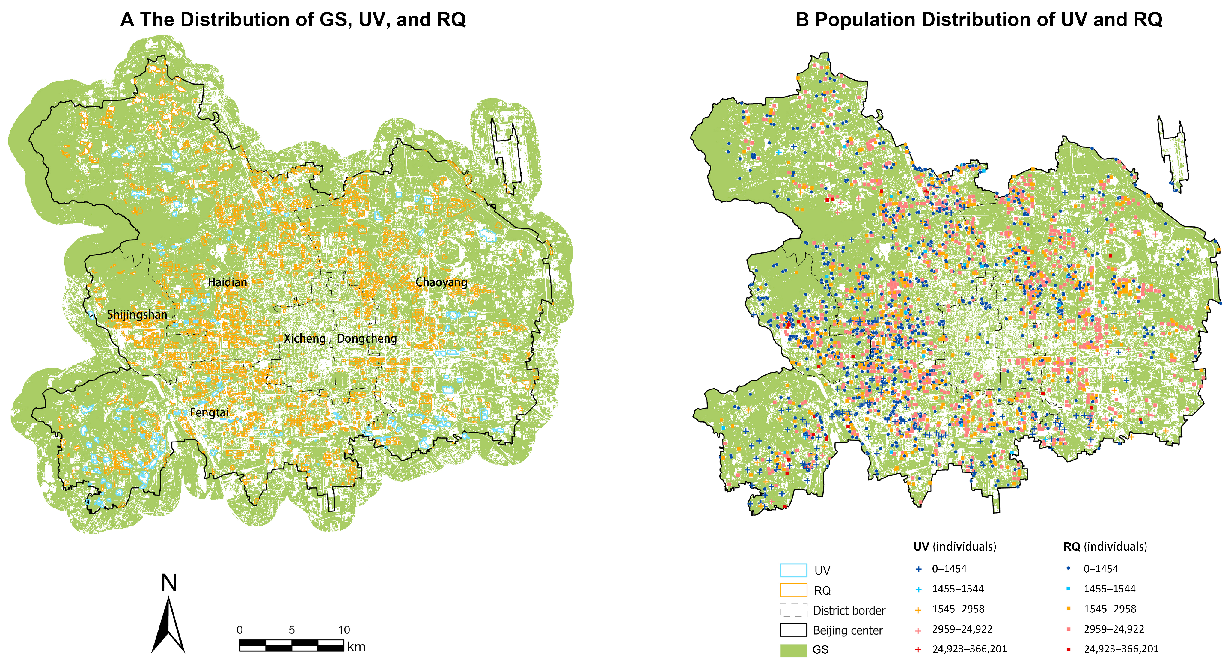
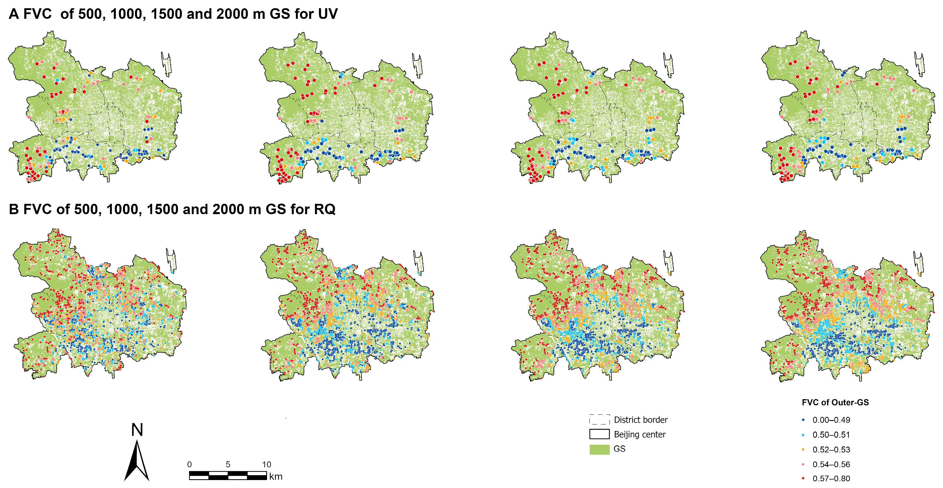
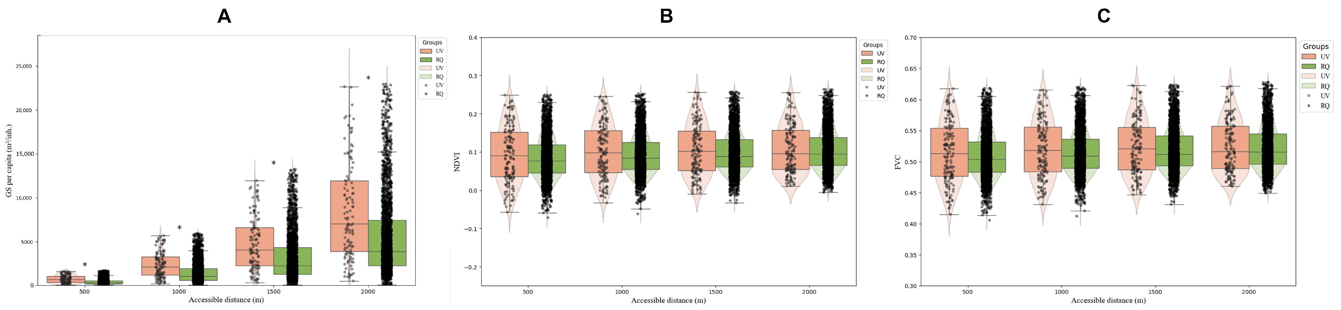
3.1. Spatial Distribution Differences in Green Space Characteristics Between UVs and RQs

The spatial distribution of RQs and UVs is illustrated in Figure 2. RQs are primarily clustered within Beijing’s central urban core, while UVs are predominantly located in peripheral and surrounding regions. with higher GS density within the urban core. In 2021, the total GS area in Beijing’s urban core was approximately 47,058.79 hectares, accounting for 34.15% of its total territory. Notably, the GS concentration was higher on the periphery of the urban core compared to other surveyed regions (Figure 1). The per capita inner GS of RQs was generally lower in the southwestern and central regions but relatively higher elsewhere, particularly in the northern areas. In contrast, the per capita inner GS of UVs was significantly higher in the southwestern region relative to other areas (Figure 2).
The spatial distribution of UVs and RQs in relation to NDVI levels is illustrated in Figure 3. The NDVI for RQs is relatively higher in the northwestern region and lower elsewhere, particularly in the southwest. Compared to per capita green space, the southeastern region shows an improvement in NDVI levels. This indicates that, although the per capita GS for RQs in this area is limited, the vegetation quality remains comparatively higher. For UVs, the NDVI levels are consistently low, suggesting that even where green spaces are relatively abundant, such as in the southwestern region, the vegetation quality remains poor.
Similarly, Figure 4 illustrates the spatial distribution of FVC for UVs and RQs. The FVC distribution mirrors the patterns observed for NDVI, with minor differences in a few neighborhoods. This suggests that FVC and NDVI exhibit similar spatial trends.
The spatial distribution characteristics of per capita inner GS, NDVI, and FVC are integrated for UVs and RQs. It is evident that NDVI and FVC show consistent trends. However, areas with higher per capita GS may not always correspond to better vegetation quality or coverage. In Beijing’s urban core, UV areas are characterized by low vegetation quality and coverage, while some UV neighborhoods in the southwestern region have relatively higher per capita GS. For RQs, the northern region consistently exhibits higher per capita GS, vegetation quality, and coverage, while the southwestern region shows lower values. Interestingly, the southeastern region displays low per capita GS but higher vegetation quality and coverage.
Figure 5 illustrates the spatial distribution patterns of external GS for UVs and RQs across distances ranging from 500 to 2000 m. Compared to internal GS, UVs in the southwestern and northwestern regions exhibit significantly higher per capita GS than other areas, while RQs demonstrate higher values in the northern regions and lower values in the south. This pattern becomes increasingly pronounced with greater distances (Figure 5).
The spatial distribution of external NDVI for UVs and RQs is shown in Figure 6. For UVs, NDVI levels increase significantly compared to internal GS, with particularly high levels in the southwestern region. This trend becomes more evident with increasing distance. In contrast, RQs display overall lower NDVI levels. While the western regions show higher NDVI than the eastern regions, this pattern is less pronounced than in the UV’s external NDVI or the RQ’s internal NDVI.
Similarly, Figure 7 shows the external FVC distribution. The spatial characteristics patterns of FVC for UVs and RQs align with those of NDVI, with consistent trends across all distances.
In summary, external green space patterns for UVs and RQs reveal that FVC and per capita GS exhibit similar trends, while NDVI shows distinct differences. The UV’s external GS performs better in the southwestern and northwestern regions across all three characteristics, whereas the southeastern region consistently underperforms. For vegetation quality, areas other than the UV’s external GS in the southwestern region require improvement. Comparing internal and external green spaces, UV areas show poor internal vegetation quality but relatively better external GS in the southwestern and northwestern regions. For RQs, both internal and external GS exhibit higher levels in the northern areas, while external vegetation quality requires further enhancement.

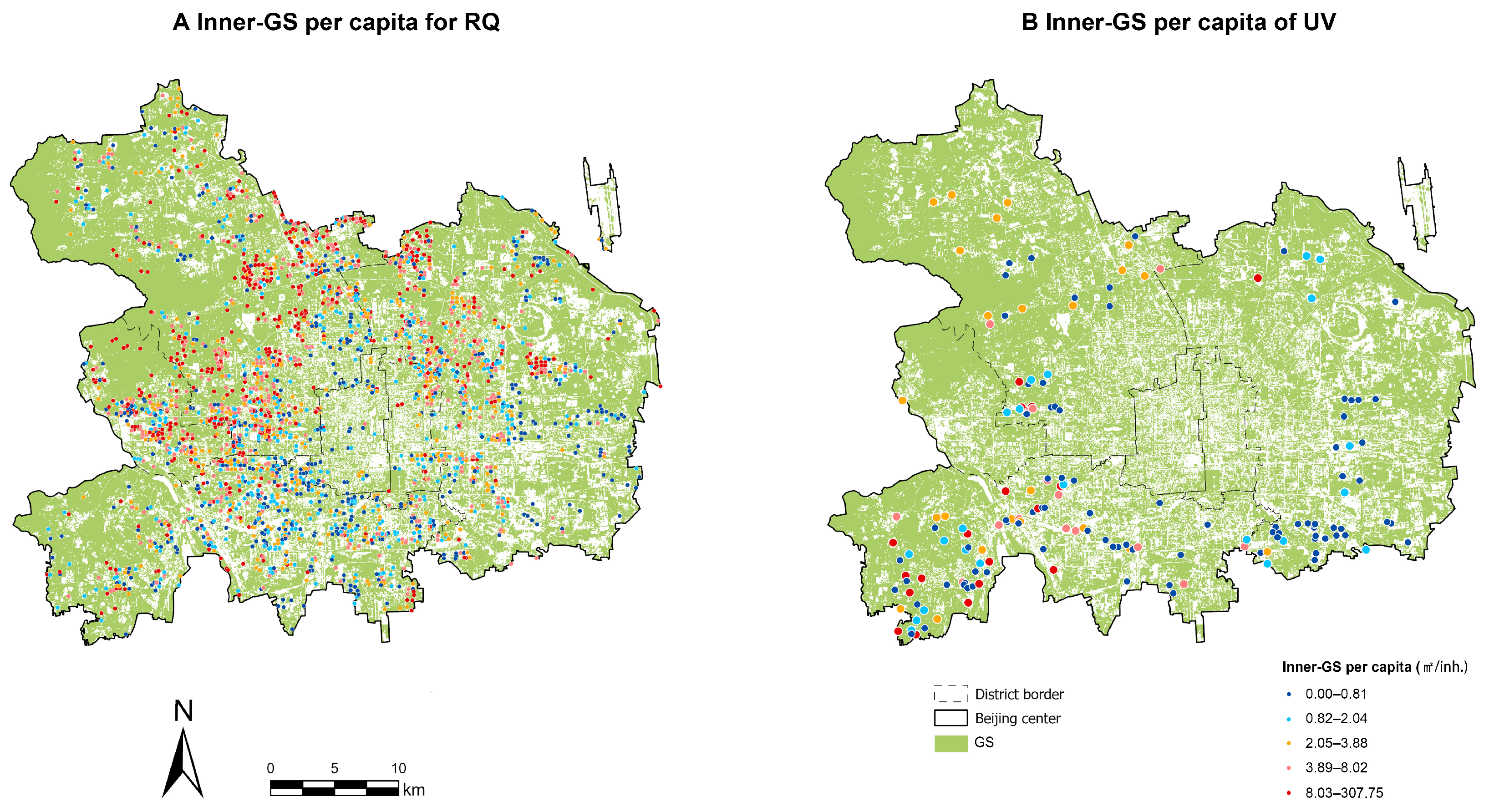
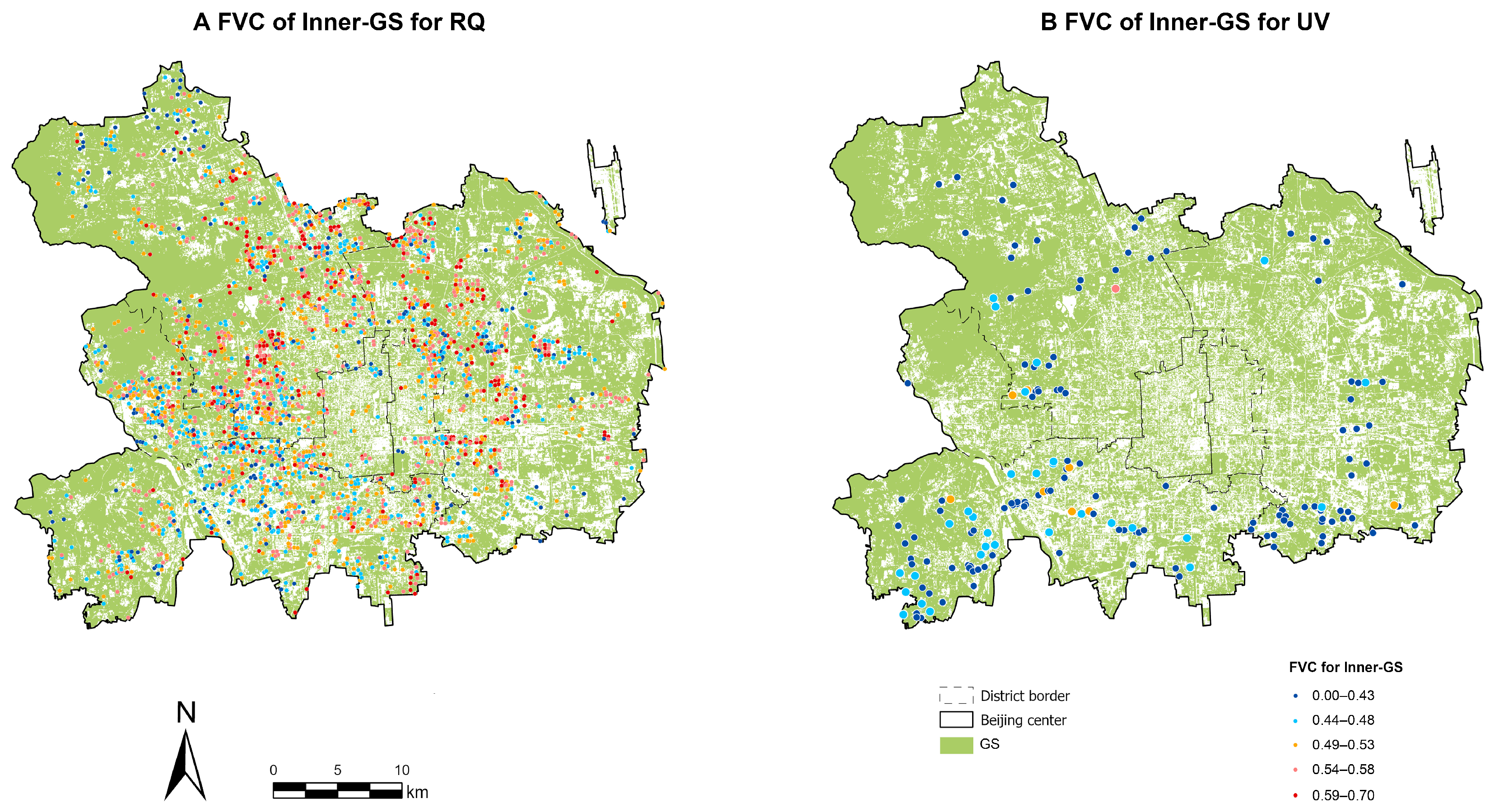
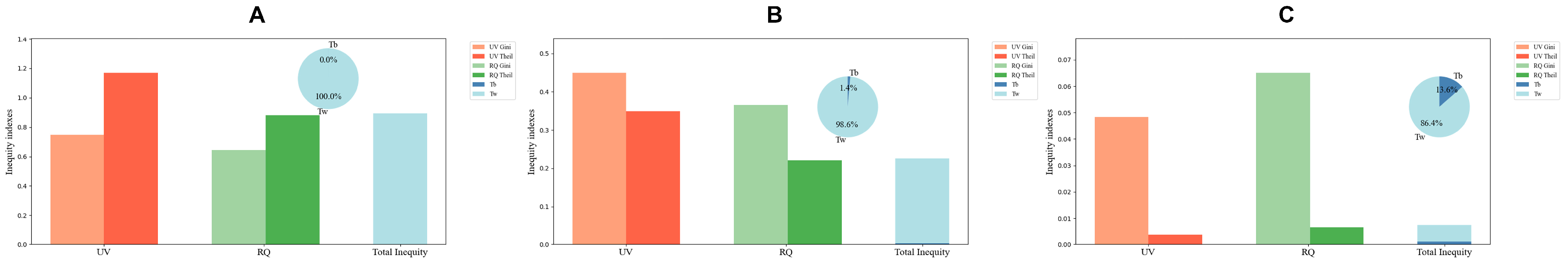
3.2. Inequalities in Inner GS Between UVs and RQs

The mean per capita inner GS for UVs and RQs was calculated as 2.89 m2/inh and 4.98 m2/inh, respectively (Figure 8). After confirming data normality and homogeneity of variance, the Mann–Whitney U test was employed to evaluate differences in per capita inner GS between the two regions. The results indicated a statistically significant disparity, with RQs demonstrating substantially higher per capita inner GS compared to UVs. Similarly, the mean NDVI values were −0.0537 for UVs and 0.0827 for RQs, again showing a significant difference favoring RQs (Figure 8). Furthermore, the mean FVC values for UVs and RQs were 0.4175 and 0.5075, respectively (Figure 8). These results consistently showed significant differences, with RQs exhibiting significantly higher inner FVC compared to UVs. Among the three green space indicators, disparities in NDVI and FVC were more pronounced across all scenarios, with RQs consistently outperforming in per capita GS availability.
This study utilized the Theil index and its decomposition to assess disparities in the distribution of inner green spaces (GSs), NDVI, and FVC. To ensure the robustness of the equity assessment, the findings were cross-validated against Gini coefficients.
The assessment of inner GS equity yielded a total Theil index of 0.8936 across all residential areas, with the within-group component contributing 0.8933 and the between-group component accounting for a mere 0.0003 (Figure 9). These findings highlight substantial disparities in GS distribution between UVs and RQs. Strikingly, within-group inequalities accounted for the entirety of the total inequity (100%), underscoring their pivotal role as the primary driver of unequal GS availability in central Beijing.
The equity assessment of NDVI revealed a total Theil index of 0.225 across all residential areas, with within-group disparities contributing 0.222 and between-group differences accounting for only 0.003 (Figure 9). The within-group index accounted for 99.07% of the total, indicating that intra-group disparities were the main driver of inequities in NDVI, contrasting significantly with the inequities in GS availability.
Regarding FVC equity, the total Theil index was 0.007, with a within-group Theil index of 0.006 and a between-group Theil index of 0.001 (Figure 9). The within-group component contributed 86.08% of the total, suggesting that intra-group disparities were the dominant factor. However, the proportion of between-group inequities was higher for FVC compared to GS availability and NDVI, reflecting a more notable contribution of inter-group differences to FVC disparities.
In summary, per capita GS and NDVI exhibited greater inequities within UVs compared to RQs, whereas FVC showed the opposite trend. A comparison using the Gini index confirmed that the results aligned with the Theil index, showing larger disparities in per capita GS and NDVI for UVs and RQs, while FVC exhibited smaller differences.

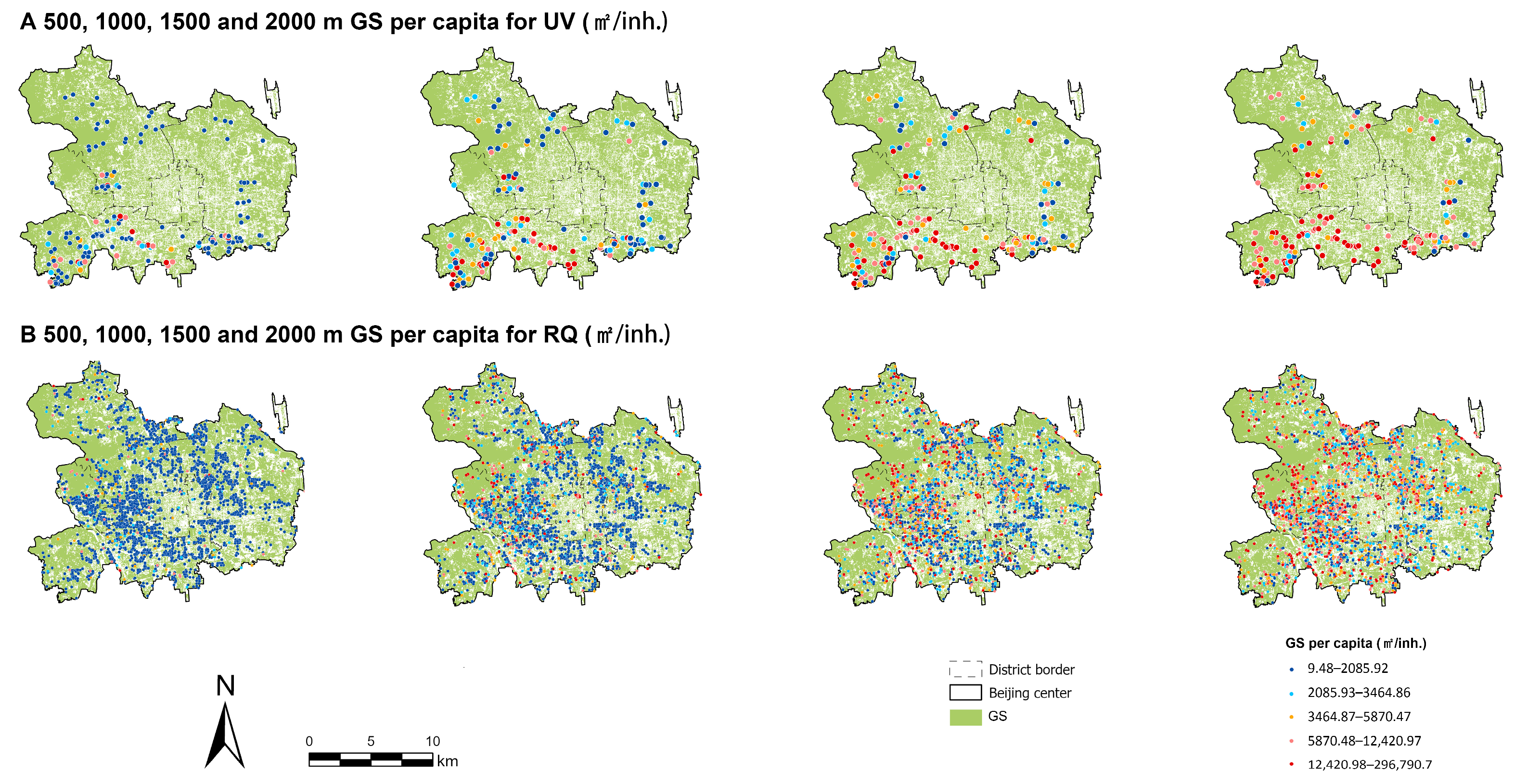
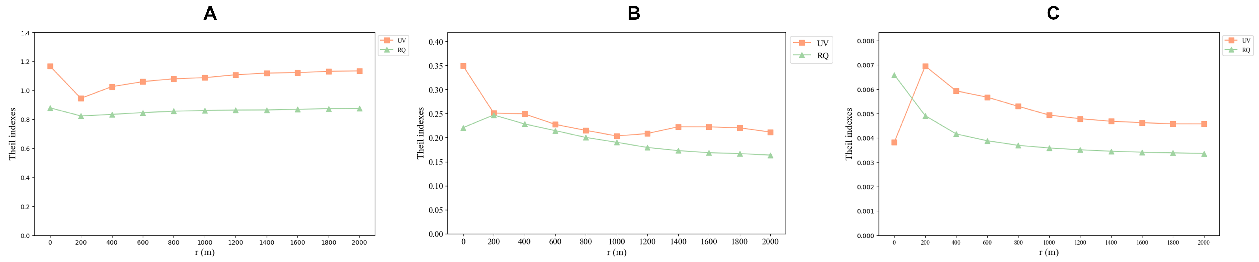
3.3. Variations in Green Space Inequalities with Accessible Distance

The analysis of external GS availability in UVs and RQs revealed a more pronounced increase in per capita GS availability for UVs as the accessible distance expanded (Figure 10). At all distances, UVs consistently exhibited greater per capita GS availability than RQs, with the disparity widening at larger distances. Likewise, mean NDVI values remained higher in UVs than in RQs across all distances, as shown in Figure 10, but the disparities were smaller compared to per capita GS and diminished with increasing distance. The analysis of FVC (Figure 10) revealed trends similar to NDVI, with UVs consistently outperforming RQs at all distances and disparities narrowing with greater accessible distances. Overall, UVs exhibited superior external green space performance across all three indicators compared to RQs.
The Theil index analysis (Figure 11) indicated that the equity of the UVs’ and RQs’ GS availability improved with accessible distance. The UV’s Theil index dropped sharply between 0 m and 100 m, suggesting improved equity, and then increased gradually with slower rates. RQs exhibited a similar but less pronounced trend. NDVI’s Theil index (Figure 11) decreased sharply between 0 m and 100 m for UVs, and then fluctuated with a peak at 1000 m and another at 1600 m. For RQs, the index rose sharply within 0–200 m but declined gradually thereafter. For FVC (Figure 11), the UV’s Theil index spiked initially but then declined at a slower rate. The RQ’s Theil index showed a rapid decrease within 0–400 m, stabilizing thereafter.
Across all three indicators, UVs and RQs displayed distinct equity trends. Notably, the UV’s NDVI equity fluctuated significantly within 1000–1600 m, while GS and FVC equity exhibited opposing trends. Overall, UVs showed greater inequities compared to RQs, except in inner FVC.
As described in Section 3.1, within-group inequities accounted for 100% of total inequities in GS availability when only internal GS was considered (Figure 9). When external GS was considered, the contribution of between-group inequities to overall inequity increased within a 200 m radius (Figure 11A). This highlights the role of external GS in reducing within-group disparities in GS availability between UVs and residential quarters (RQs). However, with increasing distance, between-group contributions declined, and within-group inequities rose.
For NDVI (Figure 12), external GS had a limited impact on mitigating within-group inequities. In contrast, FVC (Figure 12) showed a rapid decline in between-group inequities within 100 m, approaching zero, while within-group inequities surged to nearly 100%. These results emphasize the role of external GS in alleviating disparities in FVC between UVs and RQs in central Beijing.

4. Discussion

4.1. Spatial Distribution Patterns: Land Use, Planning Policies, and Capital Investment

This study reveals significant spatial disparities in GS characteristics between UVs and residential quarters (RQs). The internal green space conditions in UVs are generally poor, while external green space quality is better in the southwest and northwest but worse in the east. In contrast, RQs have higher levels of green space in the north, yet the vegetation quality of external green spaces remains low. These spatial inequalities are closely linked to land-use policies, urban planning mechanisms, and capital investment models.
From the perspective of urban political ecology (UPE), RQs are typically located in high-value urban centers, where the accessibility of green spaces is constrained by land-use regulations [73,74] While urban planning in central districts usually includes public parks, these green spaces are often capital-driven landscapes (such as parks surrounding high-end residential areas), which tend to favor specific social classes [75]. Meanwhile, UVs exist in a “gray zone” of land planning and are often excluded from the formal urban greening system, exacerbating green space inequity.
Furthermore, urban planning in Beijing’s core area has long been influenced by national macroeconomic regulation and local government land finance strategies. RQs, driven by high-end residential development, benefit from public investment in park construction, whereas UVs, due to unstable land tenure and weak planning oversight, are often excluded from such investments [76]. The green space quality in UVs is not only determined by physical spatial distribution but also deeply shaped by power relations and institutional arrangements.

4.2. Internal Distribution Patterns: Capital Accumulation and Green Space Inequality

Our study further reveals that internal green space inequality is significantly higher in UVs than in RQs, whereas FVC inequality shows the opposite trend. This phenomenon is closely related to the logic of capital accumulation in the urban land market. In RQs, real estate developers typically use high greenery levels to increase property value, whereas UVs, constrained by complex land ownership and development restrictions, have less internal green space [77].
From the perspective of capital investment, the green spaces enjoyed by RQs are often integrated with private capital cycles. For example, high-end residential communities in Beijing commonly feature private green spaces, which not only enhance residents’ living quality but also boost property market value [37]. In contrast, UVs, where land ownership belongs to village collectives, lack capital investment and public policy support, resulting in limited green space and lower internal vegetation quality.
Under the urban political ecology framework, this inequality is closely linked to power relations between the government, market, and community. Local governments tend to attract real estate investment through land sales and planning approvals, whereas UVs, constrained by limited land transfers, struggle to obtain the same level of green space allocation as RQs [76]. This disparity not only affects UV residents’ access to green spaces but also reflects institutionalized inequalities in green space distribution during urban redevelopment.

4.3. External Distribution Patterns: Systemic Inequality and Policy Implications

Our study also finds that green space inequality in Beijing’s core districts is primarily driven by intra-group inequality, rather than inter-group inequality. This phenomenon can be explained by the interaction between capital accumulation logic and environmental governance models [78].
RQs rely on high-quality park systems to enhance regional attractiveness, allowing high-end residential areas to enjoy substantial green space resources even if they are far from natural greenery [79]. In contrast, UVs—especially those in central areas—face land development restrictions, making it difficult to receive green space investments equivalent to those in RQs. Thus, the disparity in green space equity between RQs and UVs is not merely a spatial pattern but rather a result of capital flows, government interventions, and market forces. To mitigate these inequalities, policies should focus on the following directions: (1) Promoting innovative greening solutions within UVs: Strategies such as rooftop gardens, vertical greening, and street greenery can maximize the benefits of limited green space [80]. (2) Optimizing the spatial distribution of public green spaces: Particularly in UV-dense eastern and southern areas, increasing parks and open green spaces can help address UV residents’ green space shortages. (3) Establishing a socially equitable green space planning mechanism: Governments should prioritize green space needs in low-income communities during urban renewal and land planning, while setting mandatory green space allocation standards to reduce distributional inequalities [81].

4.4. Rethinking Green Space Justice in Urban Political Ecology

From an urban political ecology perspective, green space inequality is not merely a technical issue in land planning but a result of interwoven power relations, capital flows, and social inequalities [78]. Green space equity in Beijing’s core districts is shaped by three key factors: (1) Institutional constraints of land use: RQs benefit from land marketization, where green spaces are often integrated into high-end residential development, while UVs, due to their unique land tenure, cannot obtain equivalent green resources through market mechanisms. (2) Government planning biases: Urban green space policies prioritize economic growth and landscape beautification over social equity, leading to long-term neglect of green space needs in UVs. (3) Capital investment models: Green space resources in RQs are closely tied to real estate value, whereas UVs lack capital investment, resulting in lower green space quality and quantity compared to RQs.
To achieve true green space equity, urban planning must move beyond traditional technical approaches and adopt more inclusive and equitable green space policies, including incorporating green space equity into urban planning regulations to ensure fair access for all residents; redirecting capital investment towards low-income communities, using government subsidies and community engagement to improve greening in UVs and other marginalized areas; and enhancing public participation, enabling residents to play a greater role in green space planning and management to counteract power imbalances in the decision-making process [75]. By addressing these structural inequalities, cities can move towards a more just and inclusive green space distribution, ensuring that all residents—regardless of socioeconomic status—have access to high-quality urban greenery.

5. Conclusions

Investigating GS equity for disadvantaged groups is crucial for environmental justice. UVs and RQs, two common residential types in Chinese cities, present stark contrasts in GS accessibility. Ensuring equitable GS access for UV residents aligns with the United Nations’ Sustainable Development Goals on reducing inequalities, yet research on this issue remains limited.
This study examines GS equity between UVs and RQs in central Beijing, considering varying buffer distances. Findings indicate that RQs have significantly more internal GS and better equity than UVs. However, intra-community disparities, rather than differences between UVs and RQs, are the primary drivers of GS inequity. Per capita GS inequity emerges as the dominant factor shaping overall GS disparities.
Based on these findings, targeted strategies are recommended to address GS inequities in central Beijing. This research also provides broader insights into GS equity in marginalized housing typologies, including informal settlements in developing regions. From an environmental justice perspective, it highlights the need for integrating GS improvements into urban renewal initiatives, with a focus on enhancing internal GS availability for disadvantaged communities.
Despite its contributions, this study has limitations. First, it focuses on residential GS inequities but does not consider GS access in other daily environments, such as workplaces or commercial areas, which may also impact well-being. Second, it does not differentiate between GS types, such as parks or community gardens, which offer distinct benefits. Future studies should adopt a weighted evaluation approach to account for these variations. Finally, the macro-level remote sensing assessment of GS quality does not capture micro-level attributes, such as recreational facilities, safety, and aesthetic appeal, which influence usage and perceptions. Future research should integrate these aspects for a more comprehensive understanding of GS equity.

Author Contributions

Conceptualization, Q.L.; methodology, Q.L. and Y.C.; software, Q.L., M.M. and Y.C.; validation, Q.L. and Y.C.; formal analysis, Q.L.; investigation, Q.L. and Y.C.; resources, Q.L. and Y.C.; data curation, Q.L. and Y.C.; writing—original draft preparation, Q.L.; writing—review and editing, Q.L.; visualization, Q.L.; supervision, Q.L. and W.D.; project administration, Q.L. and W.D.; funding acquisition, X.Z. All authors have read and agreed to the published version of the manuscript.

Funding

This research was funded by the National Natural Science Foundation of China (No. 52208005) and the Beijing Municipal Social Science Foundation (No. 22GLC063).

Data Availability Statement

The data presented in this study are available on request from the corresponding author.

Acknowledgments

During the preparation of this work, the authors used ChatGPT-4o and DeepSeek-V3 in order to translate. After using this tool/service, the authors reviewed and edited the content as needed and take full responsibility for the content of the publication.

Conflicts of Interest

The authors declare no conflicts of interest.

Abbreviations

The following abbreviations are used in this manuscript:
UVUrban village
RQResidential quarter
NDVINormalized Difference Vegetation Index
FVCFractional Vegetation Cover

References

  1. Allegretto, G.; Kendal, D.; Flies, E.J. A systematic review of the relationship between urban forest quality and socioeconomic status or race. Urban For. Urban Green. 2022, 74, 127689. [Google Scholar] [CrossRef]
  2. Venter, Z.S.; Barton, D.N.; Gundersen, V.; Figari, H.; Nowell, M. Urban nature in a time of crisis: Recreational use of green space increases during the COVID-19 outbreak in Oslo, Norway. Environ. Res. Lett. 2020, 15, 104075. [Google Scholar] [CrossRef]
  3. Bedimo-Rung, A.L.; Mowen, A.J.; Cohen, D.A. The significance of parks to physical activity and public health: A conceptual model. Am. J. Prev. Med. 2005, 28 (Suppl. S2), 159–168. [Google Scholar] [CrossRef]
  4. Astell-Burt, T.; Feng, X.; Kolt, G.S. Mental health benefits of neighbourhood green space are stronger among physically active adults in middle-to-older age: Evidence from 260,061 Australians. Prev. Med. 2013, 57, 601–606. [Google Scholar] [CrossRef] [PubMed]
  5. Grilli, G.; Mohan, G.; Curtis, J. Public park attributes, park visits, and associated health status. Landsc. Urban Plan. 2020, 199, 103803. [Google Scholar] [CrossRef]
  6. Hartig, T.; Book, A.; Garvill, J.; Olsson, T.; Garling, T. Environmental influences on psychological restoration. Scand. J. Psychol. 1996, 37, 378–393. [Google Scholar] [CrossRef]
  7. Mitchell, R. Is physical activity in natural environments better for mental health than physical activity in other environments? Soc. Sci. Med. 2013, 91, 130–134. [Google Scholar] [CrossRef]
  8. Wolff, M.; Mascarenhas, A.; Haase, A.; Haase, D.; Andersson, E.; Borgström, S.T.; Kronenberg, J.; Laszkiewicz, E.; Biernacka, M. Conceptualizing multidimensional barriers: A framework for assessing constraints in realizing recreational benefits of urban green spaces. Ecol. Soc. 2022, 27, 17. [Google Scholar] [CrossRef]
  9. Basu, M.; Hashimoto, S.; Dasgupta, R. The mediating role of place attachment between nature connectedness and human well-being: Perspectives from Japan. Sustain. Sci. 2020, 15, 849–862. [Google Scholar] [CrossRef]
  10. Chen, Y.; Yue, W.; La Rosa, D. Which communities have better accessibility to green space? An investigation into environmental inequality using big data. Landsc. Urban Plan. 2020, 204, 103919. [Google Scholar] [CrossRef]
  11. Francis, J.; Wood, L.J.; Knuiman, M.; Giles-Corti, B. Quality or quantity? Exploring the relationship between Public Open Space attributes and mental health in Perth, Western Australia. Soc. Sci. Med. 2012, 74, 1570–1577. [Google Scholar] [CrossRef] [PubMed]
  12. Flocks, J.; Escobedo, F.; Wade, J.; Varela, S.; Wald, C. Environmental Justice Implications of Urban Tree Cover in Miami-Dade County, Florida. Environ. Justice 2011, 4, 125–134. [Google Scholar] [CrossRef]
  13. Larson, L.R.; Jennings, V.; Cloutier, S.A. Public Parks and Wellbeing in Urban Areas of the United States. PLoS ONE 2016, 11, e0153211. [Google Scholar] [CrossRef]
  14. Garizabal-Carmona, J.A.; Mancera-Rodriguez, N.J. Bird species richness across a Northern Andean city: Effects of size, shape, land cover, and vegetation of urban green spaces. Urban For. Urban Green. 2021, 64, 127300. [Google Scholar] [CrossRef]
  15. Song, P.; Kim, G.; Mayer, A.; He, R.; Tian, G. Assessing the ecosystem services of various types of urban green spaces based on i-Tree Eco. Sustainability 2020, 12, 1560. [Google Scholar] [CrossRef]
  16. Gallo, T.; Fidino, M.; Lehrer, E.W.; Magle, S.B. Mammal diversity and metacommunity dynamics in urban green spaces: Implications for urban wildlife conservation. Ecol. Appl. 2017, 27, 2330–2341. [Google Scholar] [CrossRef]
  17. Norton, B.A.; Coutts, A.M.; Livesley, S.J.; Harris, R.J.; Hunter, A.M.; Williams, N.S.G. Planning for cooler cities: A framework to prioritise green infrastructure to mitigate high temperatures in urban landscapes. Landsc. Urban Plan. 2015, 134, 127–138. [Google Scholar] [CrossRef]
  18. Skoulika, F.; Santamouris, M.; Kolokotsa, D.; Boemi, N. On the thermal characteristics and the mitigation potential of a medium size urban park in Athens, Greece. Landsc. Urban Plan. 2014, 123, 73–86. [Google Scholar] [CrossRef]
  19. Kazmierczak, A.; Cavan, G. Surface water flooding risk to urban communities: Analysis of vulnerability, hazard and exposure. Landsc. Urban Plan. 2011, 103, 185–197. [Google Scholar] [CrossRef]
  20. Speak, A.F.; Mizgajski, A.; Borysiak, J. Allotment gardens and parks: Provision of ecosystem services with an emphasis on biodiversity. Urban For. Urban Green. 2015, 14, 772–781. [Google Scholar] [CrossRef]
  21. Munoz-Pacheco, C.B.; Villasenor, N.R. Avian species richness in cities: A review of the Spanish-language literature from the Southern Cone of South America. Urban Ecosyst. 2022, 25, 601–616. [Google Scholar] [CrossRef]
  22. Chiesura, A. The role of urban parks for the sustainable city. Landsc. Urban Plan. 2004, 68, 129–138. [Google Scholar] [CrossRef]
  23. Jennings, V.; Larson, L.; Yun, J. Advancing sustainability through urban green space: Cultural ecosystem services, equity, and social determinants of health. Int. J. Environ. Res. Public Health 2016, 13, 196. [Google Scholar] [CrossRef] [PubMed]
  24. Wolch, J.R.; Byrne, J.; Newell, J.P. Urban green space, public health, and environmental justice: The challenge of making cities ‘just green enough’. Landsc. Urban Plan. 2014, 125, 234–244. [Google Scholar] [CrossRef]
  25. Crompton, J.L. Empirical evidence of the contributions of park and conservation lands to environmental sustainability: The key to repositioning the parks field. World Leis. J. 2008, 50, 154–172. [Google Scholar] [CrossRef]
  26. Harnik, P.; Crompton, J.L. Measuring the total economic value of a park system to a community. Manag. Leis. 2014, 19, 188–211. [Google Scholar] [CrossRef]
  27. Cobbinah, P.B.; Asibey, M.O.; Zuneidu, M.A.; Erdiaw-Kwasie, M.O. Accommodating green spaces in cities: Perceptions and attitudes in slums. Cities 2021, 111, 103094. [Google Scholar] [CrossRef]
  28. Pham, T.-T.-H.; Apparicio, P.; Séguin, A.-M.; Landry, S.; Gagnon, M. Spatial distribution of vegetation in Montreal: An uneven distribution or environmental inequity? Landsc. Urban Plan. 2012, 107, 214–224. [Google Scholar] [CrossRef]
  29. Nesbitt, L.; Meitner, M.J.; Sheppard, S.R.J.; Girling, C. The dimensions of urban green equity: A framework for analysis. Urban For. Urban Green. 2018, 34, 240–248. [Google Scholar] [CrossRef]
  30. Rigolon, A. Parks and young people: An environmental justice study of park proximity, acreage, and quality in Denver, Colorado. Landsc. Urban Plan. 2017, 165, 73–83. [Google Scholar] [CrossRef]
  31. Hope, D.; Gries, C.; Zhu, W.; Fagan, W.; Redman, C.; Grimm, N.; Nelson, A.; Martin, C.; Kinzig, A. Socio-economics drive urban plant diversity. Proc. Natl. Acad. Sci. USA 2003, 100, 8788–8792. [Google Scholar] [CrossRef] [PubMed]
  32. Leong, M.; Dunn, R.R.; Trautwein, M.D. Biodiversity and socioeconomics in the city: A review of the luxury effect. Biol. Lett. 2018, 14, 20180082. [Google Scholar] [CrossRef]
  33. Watkins, S.L.; Gerrish, E. The relationship between urban forests and race: A meta-analysis. J. Environ. Manag. 2018, 209, 152–168. [Google Scholar] [CrossRef] [PubMed]
  34. Macedo, J.; Haddad, M.A. Equitable distribution of open space: Using spatial analysis to evaluate urban parks in Curitiba, Brazil. Environ. Plan. B Plan. Des. 2016, 43, 1096–1117. [Google Scholar] [CrossRef]
  35. Nesbitt, L.; Meitner, M.J.; Girling, C.; Sheppard, S.R.J.; Lu, Y. Who has access to urban vegetation? A spatial analysis of distributional green equity in 10 US cities. Landsc. Urban Plan. 2019, 181, 51–79. [Google Scholar] [CrossRef]
  36. Tan, P.Y.; Samsudin, R. Effects of spatial scale on assessment of spatial equity of urban park provision. Landsc. Urban Plan. 2017, 158, 139–154. [Google Scholar] [CrossRef]
  37. Zhou, X.; Kim, J. Social disparities in tree canopy and park accessibility: A case study of six cities in Illinois using GIS and remote sensing. Urban For. Urban Green. 2013, 12, 88–97. [Google Scholar] [CrossRef]
  38. Osborn, D.; Cutter, A.; Ullah, F. Universal Sustainable Development Goals. Understanding the Transformational Challenge for Developed Countries; Stakeholder Forum: Kent, UK, 2015; Volume 2, pp. 1–25. [Google Scholar]
  39. Lopez, R.P. The Built Environment and Public Health; John Wiley & Sons: New York, NY, USA, 2012; Volume 16. [Google Scholar]
  40. Chuang, W.-C.; Boone, C.G.; Locke, D.H.; Grove, J.M.; Whitmer, A.; Buckley, G.; Zhang, S. Tree canopy change and neighborhood stability: A comparative analysis of Washington, DC and Baltimore, MD. Urban For. Urban Green. 2017, 27, 363–372. [Google Scholar] [CrossRef]
  41. Guan, J.; Wang, R.; Van Berkel, D.; Liang, Z. How spatial patterns affect urban green space equity at different equity levels: A Bayesian quantile regression approach. Landsc. Urban Plan. 2023, 233, 104709. [Google Scholar] [CrossRef]
  42. Kiani, B.; Thierry, B.; Fuller, D.; Firth, C.; Winters, M.; Kestens, Y. Gentrification, neighborhood socioeconomic factors and urban vegetation inequities: A study of greenspace and tree canopy increases in Montreal, Canada. Landsc. Urban Plan. 2023, 240, 104871. [Google Scholar] [CrossRef]
  43. Rigolon, A.; Browning, M.H.E.M.; Lee, K.; Shin, S. Access to Urban Green Space in Cities of the Global South: A Systematic Literature Review. Urban Sci. 2018, 2, 67. [Google Scholar] [CrossRef]
  44. Uribe, S.V.; Villaseñor, N.R. Inequities in urban tree care based on socioeconomic status. Urban For. Urban Green. 2024, 96, 128363. [Google Scholar] [CrossRef]
  45. Williams, T.G.; Logan, T.M.; Zuo, C.T.; Liberman, K.D.; Guikema, S.D. Parks and safety: A comparative study of green space access and inequity in five US cities. Landsc. Urban Plan. 2020, 201, 103841. [Google Scholar] [CrossRef]
  46. Zhang, P.; Park, S. Investigating spatial heterogeneity of park inequity using three access measures: A case study in Hartford, Connecticut. Appl. Geogr. 2023, 151, 102857. [Google Scholar] [CrossRef]
  47. Chawla, L. Benefits of Nature Contact for Children. J. Plan. Lit. 2015, 30, 433–452. [Google Scholar] [CrossRef]
  48. Krenichyn, K. The only place to go and be in the city: Women talk about exercise, being outdoors, and the meanings of a large urban park. Health Place 2006, 12, 631–643. [Google Scholar] [CrossRef]
  49. Rigolon, A. A complex landscape of inequity in access to urban parks: A literature review. Landsc. Urban Plan. 2016, 153, 160–169. [Google Scholar] [CrossRef]
  50. Säumel, I.; Hogrefe, J.; Battisti, L.; Wachtel, T.; Larcher, F. The healthy green living room at one’s doorstep? Use and perception of residential greenery in Berlin, Germany. Urban For. Urban Green. 2021, 58, 126949. [Google Scholar] [CrossRef]
  51. Pinault, L.; Christidis, T.; Toyib, O.; Crouse, D.L. Ethnocultural and socioeconomic disparities in exposure to residential greenness within urban Canada. Health Rep. 2021, 32, 3–14. [Google Scholar]
  52. Quinton, J.; Nesbitt, L.; Sax, D. How well do we know green gentrification? A systematic review of the methods. Prog. Hum. Geogr. 2022, 46, 960–987. [Google Scholar] [CrossRef]
  53. Hunter, R.F.; Cleland, C.; Cleary, A.; Droomers, M.; Wheeler, B.W.; Sinnett, D.; Nieuwenhuijsen, M.J.; Braubach, M. Environmental, health, wellbeing, social and equity effects of urban green space interventions: A meta-narrative evidence synthesis. Environ. Int. 2019, 130, 104923. [Google Scholar] [CrossRef] [PubMed]
  54. Lin, J.; Wang, Q. Are street tree inequalities growing or diminishing over time? The inequity remediation potential of the MillionTreesNYC initiative. J. Environ. Manag. 2021, 285, 112153. [Google Scholar] [CrossRef]
  55. Locke, D.H.; Roman, L.A.; Henning, J.G.; Healy, M. Four decades of urban land cover change in Philadelphia. Landsc. Urban Plan. 2023, 236, 104768. [Google Scholar] [CrossRef]
  56. Rigolon, A.; Flohr, T.L. Access to Parks for Youth as an Environmental Justice Issue: Access Inequalities and Possible Solutions. Buildings 2014, 4, 69–94. [Google Scholar] [CrossRef]
  57. Roman, L.A.; Conway, T.M.; Eisenman, T.S.; Koeser, A.K.; Ordonez Barona, C.; Locke, D.H.; Jenerette, G.D.; Ostberg, J.; Vogt, J. Beyond ‘trees are good’: Disservices, management costs, and tradeoffs in urban forestry. Ambio 2021, 50, 615–630. [Google Scholar] [CrossRef]
  58. Xu, C.; Huang, Q.; Su, M.; Gu, Z.; Haase, D. The inequity of urban green space availability between urban villages and residential quarters: An empirical study in Shenzhen, China. J. Clean. Prod. 2024, 448, 141704. [Google Scholar] [CrossRef]
  59. Kabisch, N.; Haase, D. Green justice or just green? Provision of urban green spaces in Berlin, Germany. Landsc. Urban Plan. 2014, 122, 129–139. [Google Scholar] [CrossRef]
  60. Low, S.; Boettcher, M. Delaying decarbonization: Climate governmentalities and sociotechnical strategies from Copenhagen to Paris. Earth Syst. Gov. 2020, 5, 100073. [Google Scholar] [CrossRef]
  61. Casey, J.A.; James, P.; Cushing, L.; Jesdale, B.M.; Morello-Frosch, R. Race, ethnicity, income concentration and 10-year change in urban greenness in the United States. Int. J. Environ. Res. Public Health 2017, 14, 1546. [Google Scholar] [CrossRef]
  62. Dong, Z.; Xia, C.; Fang, K.; Zhang, W. Effect of the carbon emissions trading policy on the co-benefits of carbon emissions reduction and air pollution control. Energy Policy 2022, 165, 112998. [Google Scholar] [CrossRef]
  63. Zheng, S.; Long, F.; Fan, C.C.; Gu, Y. Urban villages in China: A 2008 survey of migrant settlements in Beijing. Eurasian Geogr. Econ. 2009, 50, 425–446. [Google Scholar] [CrossRef]
  64. Dony, C.C.; Delmelle, E.M.; Delmelle, E.C. Re-conceptualizing accessibility to parks in multi-modal cities: A variable-width floating catchment area (VFCA) method. Landsc. Urban Plan. 2015, 143, 90–99. [Google Scholar] [CrossRef]
  65. Sharifi, F.; Nygaard, A.; Stone, W.M.; Levin, I. Accessing green space in Melbourne: Measuring inequity and household mobility. Landsc. Urban Plan. 2021, 207, 104004. [Google Scholar] [CrossRef]
  66. Browning, M.; Lee, K. Within what distance does “greenness” best predict physical health? A systematic review of articles with GIS buffer analyses across the lifespan. Int. J. Environ. Res. Public Health 2017, 14, 675. [Google Scholar] [CrossRef]
  67. Yang, G.; Zhao, Y.; Xing, H.; Fu, Y.; Liu, G.; Kang, X.; Mai, X. Understanding the changes in spatial fairness of urban greenery using time-series remote sensing images: A case study of Guangdong-Hong Kong-Macao greater bay. Sci. Total Environ. 2020, 715, 136763. [Google Scholar] [CrossRef]
  68. Abdullah, S.; Barua, D. Modeling Land Surface Temperature with a Mono-Window Algorithm to Estimate Urban Heat Island Intensity in an Expanding Urban Area. Environ. Process. 2022, 9, 14. [Google Scholar] [CrossRef]
  69. Zhang, M.; Tan, S.; Zhang, C.; Han, S.; Zou, S.; Chen, E. Assessing the impact of fractional vegetation cover on urban thermal environment: A case study of Hangzhou, China. Sustain. Cities Soc. 2023, 96, 104663. [Google Scholar] [CrossRef]
  70. Silver, W. Economics and information theory. J. Oper. Res. Soc. 1967, 18, 328. [Google Scholar] [CrossRef]
  71. Xu, C. Determinants of carbon inequality in China from static and dynamic perspectives. J. Clean. Prod. 2020, 277, 123286. [Google Scholar] [CrossRef]
  72. Cowell, F.A. On the structure of additive inequality measures. Rev. Econ. Stud. 1980, 47, 521–531. [Google Scholar] [CrossRef]
  73. Harvey, D. Justice, Nature and the Geography of Difference; Blackwell: Oxford, UK, 1996. [Google Scholar]
  74. Beijing Greening Ordinance; Government Order No. 22; Beijing Municipal People’s Government: Beijing, China, 2009.
  75. Anguelovski, I.; Connolly, J.J.T.; Masip, L.; Pearsall, H. Assessing green gentrification in historically disenfranchised neighborhoods: A longitudinal and spatial analysis of Barcelona. Urban Geogr. 2018, 39, 458–491. [Google Scholar] [CrossRef]
  76. Zhao, Y.; Webster, C. Land dispossession and enrichment in China’s suburban villages. Urban Stud. 2011, 48, 529–551. [Google Scholar] [CrossRef]
  77. Hao, P. Exploration on land development intensity of urban villages based on the bid-rent theory: A case study of Shenzhen. City Plan. Rev. 2015, 39, 24–28. (In Chinese) [Google Scholar]
  78. Swyngedouw, E.; Heynen, N.C. Urban political ecology, justice and the politics of scale. Antipode 2003, 35, 898–918. [Google Scholar] [CrossRef]
  79. Braiterman, J. City branding through new green spaces. In City Branding: Theory and Cases; Dinnie, K., Ed.; Palgrave Macmillan: London, UK, 2011; pp. 70–81. [Google Scholar]
  80. Park, H.; Brown, C.D.; Pearson, A.L. A systematic review of audit tools for evaluating the quality of green spaces in mental health research. Health Place 2024, 86, 103185. [Google Scholar] [CrossRef]
  81. Essuman-Quainoo, B.; Jim, C.Y. Understanding the drivers of green roofs and green walls adoption in global south cities: Analysis of Accra, Ghana. Urban For. Urban Green. 2023, 89, 128106. [Google Scholar] [CrossRef]
Figure 1. (A) Spatial distribution of green spaces, UVs, and RQs within Beijing’s core urban area in 2021. (B) Population distribution across UVs and RQs.
Sustainability 17 04561 g001
Figure 2. Spatial distribution patterns of per capita inner GS for RQs (A) and UVs (B).
Sustainability 17 04561 g002
Figure 3. Spatial distribution patterns of NDVI for inner GS in RQs (A) and UVs (B).
Sustainability 17 04561 g003
Figure 4. Spatial distribution of FVC within inner GS for RQs (A) and UVs (B).
Sustainability 17 04561 g004
Figure 5. Spatial characteristics of per capita GS availability for UVs (A) and RQs (B) at varying accessible distances.
Sustainability 17 04561 g005
Figure 6. Spatial characteristics of NDVI for GS availability in UVs (A) and RQs (B) across varying accessible distances.
Sustainability 17 04561 g006
Figure 7. Spatial characteristics of FVC for GS availability in UVs (A) and RQs (B) at varying accessible distances.
Sustainability 17 04561 g007
Figure 8. Average values of per capita inner GS (A), NDVI (B), and FVC (C) for UVs and RQs are presented. An asterisk above the boxes indicates statistically significant differences between UVs and RQs at the p < 0.05 level, as determined by the Mann–Whitney U test.
Sustainability 17 04561 g008
Figure 9. Inequity in inner-GS availability (A), NDVI (B), and FVC (C) for UVs and RQs, along with the decomposition of total inequities.
Sustainability 17 04561 g009
Figure 10. Mean per capita inner GS (A), NDVI (B), and FVC (C) for UVs and residential quarters (RQs). Asterisks above the boxplots denote statistically significant differences between UVs and RQs at the p < 0.05 level, as determined by the Mann–Whitney U test.
Sustainability 17 04561 g010
Figure 11. Changes in Theil indices for per capita GS availability (A), NDVI (B), and FVC (C) across UVs and RQs at progressively increasing accessible distances.
Sustainability 17 04561 g011
Figure 12. Decomposition of total inequities in per capita GS availability (A), NDVI (B), and FVC (C) between UVs and RQs at progressively increasing accessible distances.
Sustainability 17 04561 g012
Disclaimer/Publisher’s Note: The statements, opinions and data contained in all publications are solely those of the individual author(s) and contributor(s) and not of MDPI and/or the editor(s). MDPI and/or the editor(s) disclaim responsibility for any injury to people or property resulting from any ideas, methods, instructions or products referred to in the content.

