Abstract
This study aims to optimize daily forecasts of the PM2.5 concentrations in Dakar, Senegal using a long short-term memory (LSTM) neural network model. Particulate matter, aggravated by factors such as dust, traffic, and industrialization, poses a serious threat to public health, especially in developing countries. Existing models such as the Autoregressive integrated moving average (ARIMA) have limitations in capturing nonlinear relationships and complex dynamics in environmental data. Using four years of daily data collected at the Bel Air station, this study shows that the LSTM neural network model provides more accurate forecasts with a root mean square error (RMSE) of 3.2 μg/m3, whereas the RMSE for ARIMA is about 6.8 μg/m3. The LSTM model predicts reliably up to 7 days in advance, accurately reproducing extreme values, especially during dust event outbreaks and peak travel periods. Computational analysis shows that using Graphical Processing Unit and Tensor Processing Unit processors significantly reduce the execution time, improving the model efficiency while maintaining high accuracy. Overall, these results highlight the usefulness of the LSTM network for air quality prediction and its potential for public health management in Dakar.
1. Introduction
Air pollution is becoming an increasingly critical public health issue for developing countries. In the Sahel region, including Senegal, populations face a dual source of pollution, both natural and anthropogenic. Factors such as desert dust, industrial activities, and traffic emissions contribute significantly to elevated concentrations of fine particulate matter (PM) in this region, leading to severe air quality degradation. These pollutants have been linked to adverse health outcomes, as highlighted by numerous studies [1,2]. Respiratory and cardiovascular diseases are particularly influenced by exposure to fine particulate matter with a diameter below 2.5 µm and 10 µm, PM2.5 and PM10, respectively [3]. Short-term exposure, ranging from a few hours to several weeks, has been shown to increase mortality rates [4], while long-term exposure is associated with significant reductions in life expectancy, sometimes by several years [5,6].
Despite rising pollutant concentrations in major African cities, air quality monitoring and forecasting remain largely inadequate, which in fact is hindered by a lack of ground-based data and limited infrastructure for air quality surveillance. Scientific studies, sensor network installations, and the development of forecasting tools are significantly underdeveloped compared to other regions of the world, restricting the understanding of pollution dynamics over the African continent [7,8]. This gap in scientific information impedes the development of effective environmental policies, such as public awareness campaigns and regulatory frameworks, leaving populations to be exposed to significant health risks. Likewise, financial and technical constraints further limit the deployment of large-scale air pollution monitoring systems [8].
To address these challenges, the use of reliable forecasting models tailored to local contexts offers a promising solution. Effective, skillful, and accurate models are crucial to compensate for the absence of direct measurements, along with anticipating pollution peaks. However, air quality forecasting remains a major challenge due to the complexity and variability of factors influencing the atmospheric composition, such as industrial emissions, traffic pollution, and desert dust, which exhibit distinct seasonal cycles. This issue is particularly pressing, as poor air quality has well-documented links to public health crises, including respiratory and cardiovascular diseases [5].
Several approaches have been employed in Africa to forecast fine particulate matter. Traditional methods, such as statistical and physical modeling, have been proven effective but face limitations when addressing the dynamic nature of air pollution [9,10,11,12]. For example, the Autoregressive integrated moving average (ARIMA) statistical model, incorporating data assimilation, has recently been applied in Dakar for fine particulate forecasting and has yielded satisfactory and promising results [13]. While ARIMA effectively models linear trends in time series data, it struggles to capture nonlinear relationships and complex dependencies in highly variable datasets [14,15,16,17,18,19]. Conversely, machine learning techniques, particularly recurrent neural networks like long short-term memory (LSTM) models, are increasingly adopted to enhance forecasting accuracy. Indeed, these models can leverage large historical datasets and integrate various environmental parameters, offering superior capabilities to anticipate pollution episodes and their potential impacts [20]. Designed to process sequential data with long-term temporal dependencies, LSTMs excel at capturing complex, nonlinear variations by utilizing the memory mechanisms within their neurons. This capability makes LSTMs an ideal choice for analyzing air quality dynamics influenced by fluctuating factors [21,22,23]. Indeed, air pollution forecasting has been extensively explored in recent years through the application of artificial intelligence models, particularly those derived from machine learning, such as neural networks. In this context, Zhou et al. [24] proposed an attention LSTM model for solar energy prediction, which can also be adapted for air pollution modeling by accounting for seasonal variations. Other studies, such as Hu et al. [25] and Yan et al. [26], compared various environmental prediction models, highlighting the flexibility and performance of neural networks in this field. Furthermore, artificial neural networks (ANNs) have been used to model urban pollution, as demonstrated by the works of Alimissis et al. [27] and Elangasinghe et al. [28], although the limitation of available historical data remains a significant obstacle. Additionally, LSTM models incorporating filtering techniques, such as those by Pardo and Malpica [29] or Song et al. [30] with Kalman filtering, have been developed to improve air quality forecast accuracy. Finally, hybrid approaches combining LSTM and autoencoders [31], as well as LSTM Kalman or BiLSTM (bidirectional long short-term memory) models associated with empirical mode decomposition (EMD) [30,31,32,33], have yielded more precise results, even though the complexity and variability of factors influencing air quality continue to present significant challenges to modeling.
Although air quality forecasting has been extensively explored in the literature, this study is distinguished by its focus on the specific context of Senegal, a Sahelian country, and more specifically the city of Dakar. This geographic setting presents several specific challenges, including limited data availability, insufficient surface measurement infrastructure, and significant spatio-temporal variability in particulate matter concentrations, originating from both natural and anthropogenic sources. The proposed methodological approach combines data from professional fixed stations with a mobile measurement system specifically designed for this study, introducing increased complexity due to the heterogeneity of sources and challenges related to temporal synchronization. These constraints necessitated a rigorous methodological adaptation and an enhanced validation procedure, which are yet to be fully developed in prior research.
The objective of this study is to develop an LSTM model to address the limitations of our previous work [13], which was based on the ARIMA data assimilation approach, by improving both the prediction of pollution peaks and the reliability of forecasts over extended periods. Unlike ARIMA, which is reliable only up to four days, the LSTM model is expected to better integrate nonlinear trends and improve forecast accuracy for longer time horizons. This study will involve designing an LSTM model tailored to particulate matter with a diameter below 2.5 µm, hereafter PM2.5, and time series data measured in Dakar, which will serve as the training and testing datasets. Once the model is finalized and its hyperparameters are optimized following previous studies [21,22], real-time data from our platform [13] will be utilized as essential input to refine predictions. The results will be systematically compared with those obtained using the ARIMA approach to evaluate the relative performance of the two methods. This paper is organized as follows: Section 2 describes the model development, including the study area, the data processing, and the steps for the modeling development. Results and discussions are presented in Section 3. Finally, Section 4 summarizes the main findings and provides conclusions and outlooks.
2. Model Development
2.1. Data Preprocessing
2.1.1. Study Area
Figure 1 shows the study area, highlighting the Dakar area and the air quality monitoring network, consisting of specialized monitoring stations (see yellow dots). Since 2009, the Senegalese government-led Center for Air Quality Management (CGQA) has implemented an air quality monitoring system across Dakar. The network currently includes five specialized stations measuring parameters such as particulate matter (PM2.5 and PM10), nitrogen dioxide (NO2), and nitrogen oxide (NO). This study focuses on the Bel-Air station (red dot in Figure 1), the data of which will be used to train and validate the developed predictive model.
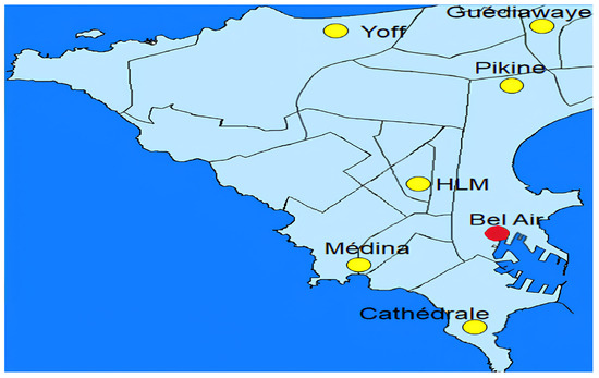
Figure 1.
Map of the city of Dakar highlighting the air quality monitoring network in Senegal managed by the Center for Air Quality Management (CGQA). The Bel Air station, the focal point of our investigation, is marked on the map by a red dot.
2.1.2. Data Processing and Organization
This study focuses primarily on daily PM2.5 data collected at the Bel Air station over a four-year period, spanning from January 2010 to December 2013. The station was selected for its high-quality and uninterrupted PM2.5 measurements over an extended duration. Overall, this study adopted a univariate approach based on the PM2.5 time series, which is mainly influenced by local sources, due to the lack of reliable ancillary data in Dakar. This strategy aims to assess the model’s performance without dependence on exogenous variables. Subsequently, the choice of the study period is based on the availability of data provided by the Senegal Air Quality Management Center, thus ensuring a reliable, continuous, and validated observation base. These data are utilized to train and validate a machine learning prediction model (LSTM) to forecast future PM2.5 concentrations. Additionally, complementary data from an automated monitoring station specifically installed for this study will be employed. The parameters measured from that automated monitoring station include PM10 and PM2.5 concentrations, as well as environmental parameters such as ambient temperature and relative humidity. These additional datasets will serve as input for a pre-identified data assimilation model, hosted on a dedicated server, to enhance the predictions of daily PM2.5 concentrations in Dakar.
The first step of this work involves preprocessing the time series data collected at the Bel Air station. The daily PM2.5 data, spanning over a three-year period, forms the foundational dataset for training and validating the prediction model. Indeed, most of the data used in this study were recorded at a daily time-scale frequency, ensuring temporal consistency across the entire analysis period. Additionally, other data from the low-cost sensor, with a finer sampling frequency of approximately 15 min, were integrated as inputs to the identified model and used for validating the generated predictions. These high-frequency data allow for a better understanding of the fine variations in PM2.5 concentrations. Furthermore, we will assess the model’s performance using standard metrics, such as the root mean square error (RMSE) and coefficient of determination (R2), directly on the daily data, without any prior aggregation. This approach ensures an accurate and rigorous evaluation of the model’s predictive capabilities, thus guaranteeing the reliability of the obtained results. Figure 2 illustrates the time series of daily PM2.5 concentrations measured at the Bel Air station between January 2010 and December 2013. As depicted in the figure, the dataset was split into two segments: the first, comprising 80% of the data (blue) (1 January 2010 through 1 December 2012), was used to train the model and tune its parameters, while the remaining 20% (green) (2 December 2012 through 31 December 2013) was reserved for testing and validating the model’s predictions.

Figure 2.
Daily PM2.5 concentration measurements from the Bel Air station used between 2010 and 2013: training data (comparison/validation) datasets are in blue (green).
2.2. Model Architecture, Training, and Conception
2.2.1. Methods
The methodology employed to develop a model tailored to the time series data from the Bel Air station consists of several essential steps, each designed to ensure the robustness and accuracy of the predictions. The process begins with data preprocessing and organization, a critical phase to guarantee the quality and consistency of the dataset. Raw data are cleaned to eliminate anomalies, outliers, or missing values, providing a reliable foundation for subsequent analysis. Once organized, the data undergoes scaling to normalize the variables. This step, typically performed using techniques such as standardization or min–max scaling, is crucial for enhancing the convergence and performance of neural networks during training. Following the scaling process, the data are transformed into a time series format. This conversion is vital for capturing sequential relationships and temporal dependencies. It enables the dataset to be structured in a way that aligns with the requirements of the long short-term memory (LSTM) models, which are particularly well-suited for analyzing time-dependent data. The next phase involves model construction, which begins with defining the basic architecture. This architecture is specifically designed to forecast future values in the time series by leveraging the trends and intricate relationships within the data. It incorporates one or more LSTM layers, selected for their ability to analyze time sequences over extended periods while retaining crucial information. These layers utilize long-term memory mechanisms to extract complex temporal features and model nonlinear variations effectively. Finally, a fully connected output layer is added to the model. This layer converts the features extracted by the LSTM layers into final predictions. In this study, these predictions correspond to the future concentrations of PM2.5. Figure 3 illustrates the flowchart and architecture of the LSTM model.
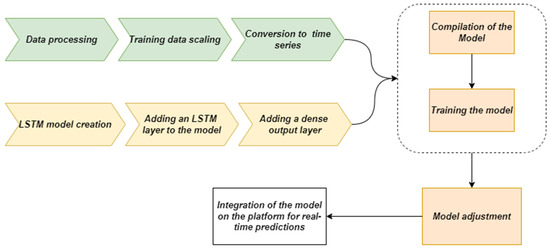
Figure 3.
Flow-chart diagram illustrating the data assimilation method steps.
The compilation and training of the model follows the construction phase. Compilation involves selecting the loss function, optimizer, and evaluation metrics that guide the learning process. These components are essential for ensuring that the model minimizes prediction errors while effectively capturing the underlying patterns of the data. It is worth pointing out that the training phase is conducted using 80% of the available data from the Bel Air station. This dataset enables the model to learn the temporal relationships and optimize its internal parameters through iterative updates. To enhance the model’s overall accuracy and performance, a fine-tuning step is carried out. During this step, adjustments to hyperparameters, such as the learning rate, batch size, or the number of LSTM units, are made. Refinements to the model’s architecture may also be introduced to better capture the dynamics of the time series. Once the model is fine-tuned, it is deployed on a dedicated platform for real-time predictions. This integration facilitates the dynamic and continuous monitoring of PM2.5 concentrations, providing an operational tool for air quality surveillance and decision-making.
2.2.2. LSTM Model
The long short-term memory (LSTM) model is a specialized recurrent neural network (RNN) architecture designed to solve the problem of learning long-term dependencies in sequential data [34]. The LSTMs show remarkable efficiency in processing time series, text, and other sequential data by storing information over long time intervals [21,35,36]. They play a key role in machine learning, especially deep learning. In time series analysis, LSTM models are used to predict future values based on past observations, making them very useful in applications ranging from finance to meteorology. LSTMs have proven to be very effective in air quality prediction by analyzing past data of pollutant concentrations, weather conditions, and other environmental factors to predict future pollution levels [37]. These predictive capabilities can help authorities and citizens make informed decisions to protect public health, such as issuing warnings when pollution levels exceed critical thresholds. LSTMs can also be integrated into real-time monitoring systems to facilitate adaptive air quality management strategies and contribute to a healthier environment [30,38]. The LSTM architecture is designed to overcome the vanishing gradient problem, a major limitation of traditional recurrent networks [21]. To achieve this, a multiplicative gating mechanism is introduced into the network structure to store and retrieve relevant information over long periods of time. LSTM cells stand out due to their complex design, which is much more advanced than that of standard RNN cells or traditional neurons. It consists of several important components, including memory cells, forgetting gates, input gates, and output gates. These components dynamically manage memory based on temporal data presented to the network [39,40]. The forgetting gate plays a fundamental role in determining whether information considered relevant at time step t – 1 should be deleted or updated at time t. Conversely, the input gate integrates new information into the memory cell at time t, even if the information was previously missing or considered less relevant at time t – 1. Finally, the output gate decides which information to transmit at the subsequent time step (t + 1) based on the internal memory state and its activation function. These three gates regulate the information flow within the LSTM cell, as shown in Figure 5 [40], optimizing temporal data processing and enabling the more accurate modeling of complex phenomena.
2.2.3. Configuration of the LSTM Model
The configuration of the LSTM model depends on various parameters and hyperparameters that have a significant impact on the performance of modeling time series and other sequential data. Given the specific characteristics of the dataset and the prediction objective, it is essential to optimally tune these factors to maximize the model performance. As shown in Table 1, the key parameters determine the architecture and capabilities of the LSTM model to capture the temporal dependencies of air quality time series. As highlighted by [21,41,42], these structural parameters enable the model to detect complex patterns that are important for accurate predictions in dynamic environments. This ability to identify complex temporal relationships is particularly important in areas such as air quality monitoring, where system dynamics are often driven by multiple interdependent factors.

Table 1.
Parameters characterizing the LSTM model.
As for the hyperparameters, detailed in Table 2, they directly impact on the training process and the optimization of the model. A careful selection of the batch size and the number of epochs is critical to achieving an optimal balance between computational efficiency and predictive accuracy. An appropriately chosen batch size enables efficient resource management while ensuring stable model convergence, whereas an adequate number of epochs maximizes the learning of data representations while avoiding overfitting [43,44]. These adjustments are fundamental for enhancing the model’s predictive capacity while minimizing errors, including bias and variance, thereby ensuring a robust generalization to unseen data.
Table 2.
Hyperparameters of the LSTM Model.
2.3. Selection of the Optimal LSTM Model
This section provides a detailed description of the tuning process of the basic parameters and hyperparameters of the LSTM model using a systematic approach to optimize its performance on predicting fine matter concentrations in Dakar. The main goal is to systematically calibrate these parameters to achieve an optimal balance between prediction accuracy and computational efficiency.
2.3.1. Sequence Length
The first parameter analyzed is the sequence length, which is defined as the number of time steps the model considers for each input sample. This parameter is very important because it allows the model to capture the temporal dependencies and patterns of variation present in the air quality data. For instance, Figure 4 shows the evolution of the root mean square error (RMSE) as a function of the sequence length used for the LSTM model applied to the PM2.5 concentration dataset recorded at the Bel Air station. This curve highlights the importance of determining an optimal sequence length that effectively incorporates relevant temporal information without incurring an overload from excessive historical data. The analysis shows that sequence lengths of 10, 20, 30, and 40 effectively capture the main temporal dependencies while avoiding the significant increase in RMSE observed with longer sequences [47,48,49].
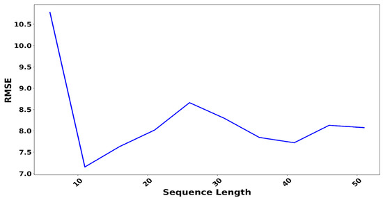
Figure 4.
Variation in sequence length as a function of the root means square error (RMSE).
2.3.2. Batch Size
When designing an LSTM model, deciding on the batch size is a crucial step. In the context of LSTM networks, this parameter represents the number of data samples processed simultaneously to update the network weights during the training phase [33]. Figure 5 shows the relationship between the previously determined sequence length and the batch size based on the RMSE indicator for the LSTM model trained on the Bel Air data. Each cell in the Heatmap represents the RMSE value obtained for a specific combination of the sequence length (seq10, seq20, seq30, seq40) and batch size (1, 5, 10, 16, 32, 64, 128). The results show that, regardless of the sequence length, a larger batch size (16, 32, 64, or 128) is generally better at minimizing the RMSE. However, further minor improvements can be achieved by fine-tuning these two hyperparameters to take into account the trade-off between computational cost and accuracy [50].
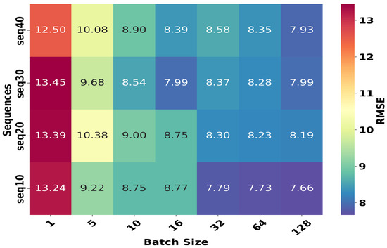
Figure 5.
Heatmap of RMSE to illustrate the optimization of batch sizes based on sequence length.
2.3.3. Determination of the Number of Layers and Neurons
In this section, we determine the optimal number of neurons for the first layer of the neural network applied to the PM2.5 concentration data of the Bel Air station in Dakar. Figure 6 shows the relationship between the optimal sequence length determined in the previous step and the number of neurons in the first layer estimated using the RMSE metric. The results show that increasing the number of neurons significantly improves the prediction accuracy by decreasing the RMSE. In particular, the 500-neuron configuration shows the optimal performance, with RMSE values ranging from 7.36 to 8.78 μg/m3, depending on the sequence length. In contrast, the simple configuration with 50 to 100 neurons shows a much higher error, exceeding 14 μg/m3. These results highlight the need for architectures that are sufficiently complex to capture nonlinear data dynamics [51]. However, performance appears to plateau after 500 neurons, and increasing the number of neurons does not significantly improve the RMSE. Overall, in line with the previous study by Salman [52], our result suggests a trade-off between model complexity and prediction performance, where further increases in the number of neurons yield modest improvements in accuracy.
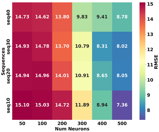
Figure 6.
Heatmap of RMSE illustrating the variation in the number of neurons in the first layer based on different sequence lengths.
2.3.4. Iteration
In long short-term memory (LSTM) models, the number of epochs play a crucial role in the learning process by iteratively updating the network weights to minimize prediction errors and capture complex temporal dependencies [53]. Striking the right balance in the number of epochs is essential: too few epochs result in underfitting, where the model fails to learn key patterns, while too many epochs lead to overfitting, diminishing the model’s ability to generalize to new data [54,55,56].
This delicate trade-off is clearly illustrated in Figure 7, which shows how performance metrics—R2 in Figure 7a and RMSE in Figure 7b—evolve with increasing epochs and varying input sequence lengths. Notably, both metrics improve as epochs increase, with the most significant gains observed around 400 epochs. At this point, sequences of length 10 and 20 achieve RMSE values below 7 and R2 values close to 0.96, indicating strong predictive accuracy. In contrast, shorter sequences like seq1 consistently underperform, highlighting the importance of an adequate sequence length in modeling temporal dynamics. Overall, these observations confirm findings by Freeman [57] and emphasize that training beyond 400 epochs offers limited improvement and risks overfitting, reinforcing the need for the careful tuning of the training duration in LSTM models.
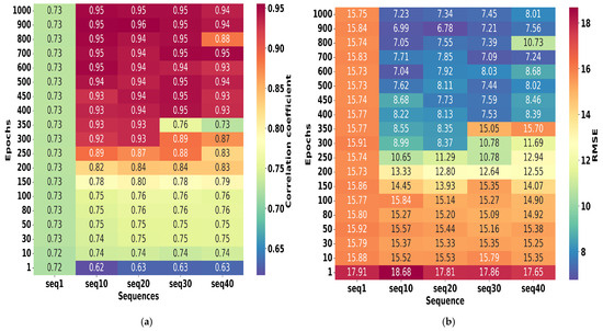
Figure 7.
Heatmap of correlation coefficient [on the left, (a)] and RMSE [on the right, (b)] illustrating the variation in the number of epochs with respect to different sequence lengths.
2.3.5. Hyperparameters
When designing the LSTM model, we determined that the Adaptive Moment Estimation (ADAM) optimizer and a dropout rate of 0.2 were the optimal hyperparameter choices to maximize model performance. These choices are based on strong theoretical foundations and previous studies that have demonstrated their effectiveness.
- The ADAM optimizer, introduced by Kingma [58], is well known for its performance on deep learning models, especially recurrent architectures such as LSTM. The ADAM optimizer combines the benefits of the root mean square propagation (RMSProp) and Stochastic Gradient Descent (SGD) optimizers with first and second moment corrections to dynamically adjust the learning rate. This adaptability ensures fast and stable convergence even in environments with complex or noisy gradients.
- A dropout rate of 0.2 has been shown to be important in preventing overfitting. This method, introduced by Hinton and further investigated by Srivastava [59], involves randomly disabling 20% of the neurons at each training step. This reduces dependencies between neurons and promotes better generalization while maintaining a balance between model complexity and robustness. The value of 0.2 is chosen as an optimal compromise, ensuring high performance while minimizing the risk of overtraining.
2.3.6. Model Architecture
The results summarized in Table 3 show the neural network architecture with a sequence length of 30, batch size of 16 with 500 training epochs, an ADAM optimizer, a dropout rate 0.2, and 500 neurons among the tested configurations. The first layer provided the best performance. This configuration achieved an RMSE of 7.44 and coefficient of determination (R2) of 0.95, indicating the model’s strong ability to predict the complex temporal evolution of the data with high accuracy.
Table 3.
Performances of the LSTM model.
2.3.7. Model Adjustment
After generating the basic configuration of the model, a new optimization was performed by including a second neural layer to improve performance. The goal of this step is to adjust the number of neurons in each layer to achieve a balance between learning and generalization while avoiding underfitting or overfitting. Adding this second layer allows the model to capture more complex features, which is important for the efficient modeling of nonlinear time series. Our test results show that the optimal configuration is achieved when the number of neurons in the second layer is kept relatively low (around 50 or less). Figure 8 shows a clear trend where the RMSE remains low and when the number of neurons in the second layer is between 0 and 50. Increasing the number of neurons beyond this threshold results in a marked increase in the RMSE, indicating an increased risk of overfitting. This finding highlight that despite the obvious appeal of more complex neural architectures, the controlled simplification of neural layers often helps improve generalization and maintain optimal performance [52].
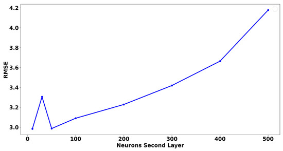
Figure 8.
Variation in RMSE based on the number of neurons in the second layer.
2.3.8. Impact of Sequence Length on the Model’s Predictive Performance
Based on the model parameters, we performed particulate matter concentration predictions using the following four specific sequence lengths: 10, 20, 30, and 40. Figure 9 shows the forecast performed by the model for each sequence length. Specifically, Figure 9a–d shows the simulation with sequence lengths 10, 20, 30, and 40, respectively. In each graph, the blue curve represents the training data on the left side and the test data on the right side. This difference allows us to test the model’s predictions by comparing the observed values on the test data with the predictions generated by the model. These simulations provide detailed insight into the model’s performance across a range of sequence length configurations. The results show a good agreement between observed and predicted values, highlighting the model’s ability to capture trends in the data used for training. However, while predictions generally follow observed trends, there are notable discrepancies during rapid changes in the data. This discrepancy highlights the model’s limitations in adapting to rapid and unexpected changes in the time series data that were not observed during training. The effect of the sequence length is also evident. For short sequences, such as 10, the model responds quickly but struggles to effectively model long-term timing dependencies. In contrast, using longer sequences, such as 40, improves the capture of complex temporal relationships, but the increased complexity may degrade performance, especially during rapid fluctuations. These observations highlight the importance of choosing the optimal sequence length while balancing responsiveness and modeling long-term dependencies. Therefore, a deeper analysis of these numbers suggests that intermediate sequence lengths, such as 20 or 30, represent an optimal compromise while effectively balancing prediction accuracy and model robustness.
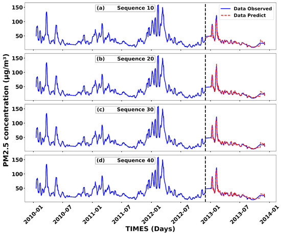
Figure 9.
Prediction of PM2.5 concentrations (in red) for the four selected sequence lengths: (a) 10, (b) 20, (c) 30, and (d) 40. The blue curve represents the observations used as input and validation data.
Table 4 summarizes the performance of each LSTM model configuration based on different sequence lengths. It includes the RMSE, coefficient of determination (R2), running time, and CPU memory usage associated with each configuration. These metrics assess not only the accuracy of the model but also its computational efficiency, providing a comprehensive overview of the model’s performance in different training scenarios.
Table 4.
Performance indicators of the model based on the four sequence lengths.
The results show that intermediate sequence lengths (20 and 30) provide an optimal balance, offering a favorable trade-off between prediction accuracy (low RMSE), high coefficient of determination (R2), and moderate resource usage, especially in terms of computation time and CPU memory. In particular, the configuration with a sequence length of 20 achieves the optimal balance with R2 of 0.989 and RMSE of 3.00, as well as a residual mean of 0.10, and a standard deviation of 2.29, while keeping the computational cost reasonable. In contrast, increasing the sequence length (e.g., to 40) significantly increases the running time without any noticeable performance gain, emphasizing the trade-off between accuracy and complexity when choosing model hyperparameters. Indeed, the evaluation of CPU memory usage during execution was performed using the Python 3.12.0 library “psutil (python system and process utilities)”, which is known for its reliability in monitoring system resources [60].
Finally, the LSTM model used is based on two stacked layers with 500 and 50 neurons, with a dropout rate of 0.2. The training is performed over 500 epochs with a batch size of 16, using the ADAM optimizer and the MSE loss function. Once trained, the model is loaded to make predictions without further learning phases. The datasets are normalized using the same parameters as during training, then organized into time sequences of 20 steps. Each sequence generates a prediction, which is then denormalized to recover the actual scale.
2.3.9. Architecture and Configuration of the LSTM Model
Through a series of in-depth analyses and methodological adjustments, we determined the optimal architecture for the LSTM model, as listed in Table 5. The selected sequence length of 20 provides an ideal balance between prediction accuracy and computational efficiency. In 500 iterations, the model converges steadily while avoiding overfitting, ensuring optimal performance. The batch size of 16 was chosen to maximize the efficiency of the training process without compromising the quality of the results by achieving the balanced management of training resources and performance, as suggested by Hague [61]. The architecture consists of two layers. The first layer contains 500 neurons, which provides a significant learning ability for extracting complex features, while the second layer contains 50 neurons to maintain structural simplicity and promote efficient generalization. This configuration demonstrates high prediction accuracy, achieving an RMSE of 3.00 with an R2 of 0.989 on the test data. From a resource perspective, this setup has proven to be efficient, with a runtime of 44 min and a maximum CPU memory usage of 0.54 GB. The loss curves for both the training and validation sets (Figure 10) reveal a stable convergence of the model after approximately 400 epochs, with a gradual and synchronized reduction in prediction errors across both sets. The absence of divergence between the two curves, along with the plateauing of losses without a significant rebound, indicates that no overfitting is observed. This behavior reflects the model’s robust generalization ability, demonstrating the efficient weight optimization and appropriate regularization of the LSTM architecture. These optimizations reflect an ideal balance between performance, stability, and resource efficiency, making the model well-suited for processing complex time series data.
Table 5.
Optimal configuration of the LSTM model.
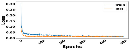
Figure 10.
Loss dynamics during the training of the sequential model.
Figure 11 shows the evolution of PM2.5 concentrations, highlighting the model performance for a sequence length of 20. The blue curve represents the training data used to tune the model parameters, while the green curve corresponds to the test data used to evaluate the generalization ability of the model. The predictions made by the model based on the test data are shown in the red dot–dot curve. This visualization makes it easier to evaluate the agreement between the actual observations and the model predictions, and analyze potential discrepancies, especially when PM2.5 concentrations change abruptly. The results show that the model effectively captures trends and changes in PM2.5 concentrations, including significant fluctuations, reflecting the ability of the model to reproduce the temporal dynamics of the data. The consistency observed between the actual data and the predictions highlights the accuracy of the model in capturing the phenomenon under study. This performance highlights the effectiveness of the chosen architecture in monitoring and predicting fine particle concentrations and further validates the relevance of the chosen configuration.
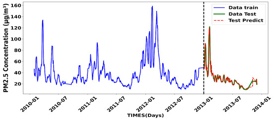
Figure 11.
Prediction with the optimal LSTM model.
3. Results and Discussion
After determining the optimal LSTM model configuration for the PM2.5 dataset measured at the Bel Air station, we performed an in-depth performance evaluation for future forecasting. The purpose of this analysis is to evaluate the robustness of the model and its ability to accurately represent the complex dynamics of environmental time series, especially with respect to PM2.5 concentrations. The results of this study are compared with those obtained from our previous studies, particularly using the ARIMA (3, 0, 1) data assimilation model [13]. The main goal is to investigate the extent to which the LSTM model outperforms or is outperformed by the ARIMA model by focusing on the accuracy of the representation of extreme values, both maximum and minimum.
3.1. Model Performance over a 10-Day Period
To evaluate the performance of the LSTM model, predictions were run for 10 consecutive days. Figure 12 displays the model performance statistics, showing the RMSE (Figure 12a) and the coefficient of determination (R2, Figure 12b), over the entire 10-day prediction period. The results show that the LSTM model achieves high performance from day 1 to day 6, with an RMSE of less than and exceeding 91%. However, from day 7 onwards, we notice a decline in the performance, characterized by an R2 value that drops to about 72%, with an RMSE of by day−10. These results highlight the robustness of the LSTM model for predictions up to a week in advance.
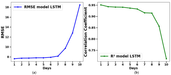
Figure 12.
Daily fluctuation in root means square error (RMSE) (a) and correlation coefficient (R2) (b) between predictions and measurements.
3.2. Comparative Analysis with the ARIMA Data Assimilation Model
To evaluate the relevance of the LSTM model compared to other models, we compared the performance of the ARIMA data assimilation model with that of the LSTM model for the same PM2.5 data series from the Bel Air station. Figure 13 displays a Taylor diagram summarizing various statistical metrics (RMSE, R2, and standard deviation) for the two models over an 8-day forecast period. The Taylor diagram allows us to simultaneously analyze the correlation between the model and the observations, the standard deviation, and the RMSE, providing a comprehensive assessment of their performance. Overall, the results show that the LSTM model significantly outperforms the ARIMA. This superiority is highlighted by the fact that the standard deviation of the LSTM predictions is less than, which is closer to the baseline and RMSE values during the first 7 days. In addition, the correlation coefficient of the LSTM model exceeds 0.92, confirming its reliability. In addition, the dynamics of the two models are noticeably different. The LSTM model maintains high performance for the first 7 days before converging to the mean. In contrast, the ARIMA model showed high performance only on the first day, then declined sharply and stabilized at a constant level close to the mean [62].
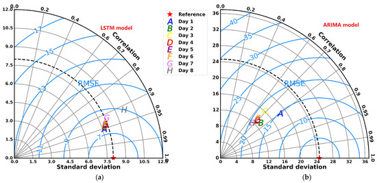
Figure 13.
Taylor diagram providing three statistical scores (standard deviation, correlation coefficient, and root means square error) between measurements and model predictions over an 8-day period. (a) shows the indicators generated using the ARIMA data assimilation model, while (b) displays the results from the LSTM model.
Table 6 shows the statistical performance of the two models for the 7-day forecast, comparing the PM2.5 concentration prediction performance in Dakar. The results show that the LSTM model has a high R2, ranging from 0.92 to 0.95, indicating excellent agreement between the predictions and actual observations. In contrast, the ARIMA model shows a low R2 value, ranging from 0.65 to 0.80, reflecting a less accurate modeling of the underlying relationship. In addition, when analyzing the RMSE, the LSTM model also outperforms the ARIMA model in terms of prediction accuracy. For instance, under the LSTM model, the RMSE values range from 7.63 to, while the ARIMA model values are in the range of 14.99 to. Overall, these results highlight the superiority of the LSTM model over the ARIMA model. Thus, the LSTM model provides more reliable predictions that closely match actual observations.
Table 6.
Comparison of performance indicators between the LSTM model and ARIMA over 7 days predictions.
3.3. Forecasting Using Data from Automatic Stations as Input
In this section, we address the daily prediction step using the developed and validated LSTM model. Data from the automated PM2.5 measuring station in Dakar [13] were used as input and test data for the model. To consider fluctuations in PM2.5 concentrations throughout the day, a daily average was calculated based on measurements taken every two hours [63]. The forecasting period is from March to July 2024. Figure 14 shows the predictions made by the LSTM (red) and the ARIMA (green) models during this period compared to the control data measured at the automated station (blue curve). Note that the reference data were used as both the input and test basis for both models. In this first setup, daily input data from automatic stations were provided to predict PM2.5 concentrations for the next few days. The results show that both models accurately capture the overall daily trend. However, the LSTM model stands out for its higher accuracy in reproducing extreme values, such as maximum and minimum values observed during the analysis period. These results are in line with previous studies [64,65].
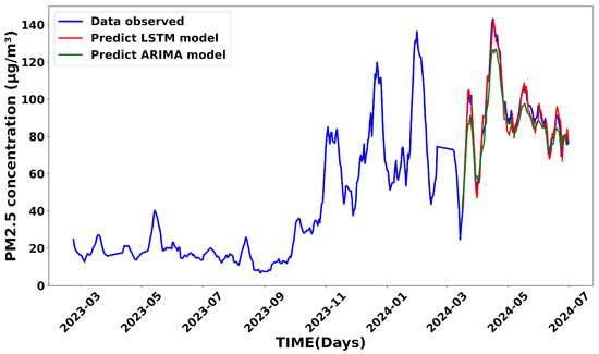
Figure 14.
Daily forecasts generated by the LSTM and ARIMA models, covering the period spanning from March to July 2024.
Table 7 shows that the differences become more obvious when comparing various statistical metrics of the two models, particularly on extreme values recorded at the Bel Air station. This highlights the importance of selecting the most appropriate model based on the specific characteristics of the data and monitoring objectives. Overall, the LSTM model stands out with a difference of between the observed and predicted values for the maximum concentration, and a mean difference of reflecting greater accuracy and stability in predictions. In contrast, the ARIMA model exhibits significantly larger discrepancies, with a maximum difference of 16 µg/m3 and a mean difference of 3. In terms of correlation, the R2 for the LSTM model reaches 0.97, indicating excellent agreement between observed and predicted values. Conversely, the ARIMA model shows a lowered correlation, with an R2 of 0.79. Regarding the overall errors, the LSTM model achieves an RMSE of whereas the ARIMA model’s RMSE is. In summary, Figure 14 combined with Table 7 further demonstrates the ability of the LSTM model to more accurately capture the complex dynamics of PM2.5 concentrations, thus emphasizing its relevance for environmental monitoring applications. Overall, the LSTM model proves to be an essential tool for precise monitoring and informed decision-making in air quality management.
Table 7.
Statistical comparison of measured extreme values and predictions of LSTM and ARIMA models.
Figure 15 shows the PM2.5 concentration predictions for 7 days with the initial input taken from the automatic station in order to start the predictions. Likewise, Figure 14 shows the predictions generated by the two approaches starting from the starting point of the input data (marked by the black star) and compares them to the actual observations shown by the blue curve. In fact, here, from day 3, the model continues the calculations until day 7 but relies only on the previous day’s predictions [66]. The results show that both models predict PM2.5 concentrations relatively well for the 7-day periods. However, LSTM model predictions are more efficient and compare better to the observation than the ARIMA model predictions, especially when it comes to capturing extreme values.
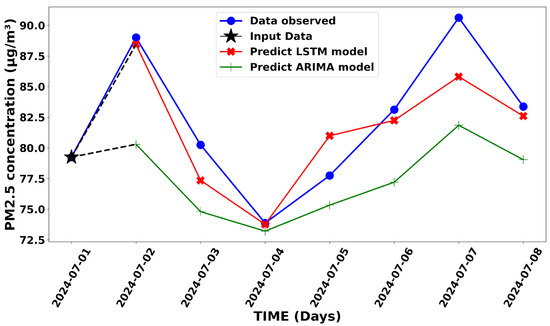
Figure 15.
Simulation of 7-day prediction using LSTM and ARIMA models.
To evaluate the fit of the LSTM and ARIMA models against the real/observed data, we performed a linear regression using the previous predictions. Figure 16 shows this fit by visually comparing the regression lines associated with each model. The predicted days are numbered from one to seven. The regression line for the daily observations of the automatic station considered as the reference is shown in yellow, while the actual measurements are shown in blue. The daily predictions and regression lines for the LSTM (ARIMA) model are shown in red (green). The LSTM model is highlighted by its regression equation , which indicates a relatively close relationship to the baseline (yellow). However, the slope is slightly less than 1 and the positive intercept indicates that it underestimates higher values, especially in extreme cases. In comparison, the ARIMA model has a regression equation of, with a slope that deviates significantly from the baseline. These results highlight the tendency of ARIMA models to overestimate low values and underestimate high values, reflecting their limitations in capturing the complex variation present in the observations.
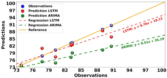
Figure 16.
Comparison of LSTM and ARIMA Models’ performance via linear regressions on real data for prediction days.
3.4. Characterization of LSTM Model Performance Zones Based on Computational Resource
Hardware resources play an essential role in the training and running of deep learning models such as LSTM, balancing accuracy, speed, and efficiency [67]. The choice of platform should match the nature of the data and the specific requirements of the project. Whether the goal is fast real-time execution or the precise optimization of mission-critical applications, resource selection has a significant impact on performance. Table 8 provides a detailed comparison of the performance of LSTM models on different platforms, considering parameters such as RAM size, processor type (GPU, TPU, or CPU), and execution time. This analysis highlights the impact of hardware on key statistics such as the RMSE and coefficient of determination (R2). The results show that GPU platforms such as Colab T4 GPU provide the best balance between speed and accuracy. With a runtime of 5 min and 40 s and an RMSE of 3.48, this configuration is particularly suitable for environments that require fast response times. TPU processors require more time (25 min) but are highly accurate, achieving a lower RMSE (2.88) and higher R2 (0.99), making them ideal for high-reliability analyses. CPU platforms, including Kaggle Server, Colab, and local environments, exhibit longer runtimes (ranging from 37 to 79 min depending on the configuration) but maintain an acceptable level of accuracy. For example, Kaggle Server achieves an RMSE of 2.92 and an R2 of 0.99, showing that CPUs can be a viable alternative for resource-constrained projects. This comparison highlights the tradeoff between speed and accuracy inherent in each resource type. Both GPUs and TPUs are better-suited for computer-intensive tasks or high-precision requirements, while CPUs are still a low-cost option for less demanding situations. The analysis highlights the importance of selecting appropriate hardware resources based on specific design goals and constraints.
Table 8.
Analysis of LSTM model execution performance based on computational resources.
4. Conclusions and Outlook
The goal of this study was to develop an LSTM model capable of capturing nonlinear variations in fine particulate matter concentrations in the Dakar area of Senegal. It builds upon previous work by [13], employing ARIMA-type data assimilation models, which are effective for 4-day forecasts but exhibit significant bias, especially for extreme measurements. To address these limitations, an LSTM model was developed using data from the Bel Air broadcasting station, with the dataset split into training (80% of the datasets) and evaluation (20% of the datasets) phases. The optimal LSTM configuration included a sequence length of 20, a batch size of 16, training for more than 500 epochs, the ADAM optimizer, a dropout rate of 0.2, and a neural architecture with 500 neurons in the first layer and 50 neurons in the second layer. The performance evaluation showed that the LSTM model significantly outperformed the ARIMA model. In particular, the LSTM provides reliable forecasts for up to a week, while the ARIMA model forecasts tend to converge to the mean as early as day 3. Statistical performance further confirms this superiority, with the LSTM model achieving much lower RMSE values and higher coefficient of determination values (R2 exceeding 97%). In addition, our results show that the LSTM models have a remarkable ability to accurately reproduce extreme values, such as dust storm outbreaks or peak hours related to urban traffic. This analysis also highlights the important role of computational resources in optimizing model performance. Using GPUs and TPUs significantly reduces the execution times while maintaining high levels of accuracy. These results highlight the importance of investing in advanced computing technologies to improve the performance of predictive models used in air quality management. Although the model used in this study is univariate, future approaches could incorporate interpretability techniques such as attention mechanisms, LIMEs (Local Interpretable Model-agnostic Explanations), or SHAPs (SHapley Additive exPlanations), to identify the most influential temporal sequences in PM2.5 concentration predictions.
Author Contributions
Conceptualization, A.G., I.D. and M.S.D.; methodology, A.G., S.A.A.N., I.D. and M.S.D.; software, A.G. and S.A.A.N.; validation, A.G., S.A.A.N., I.D., M.S.D., M.D. and A.A.Y.; formal analysis, A.G., S.A.A.N. and M.S.D.; investigation, A.G., I.D. and M.S.D.; resources, I.D., M.S.D. and M.D.; data curation, A.G., S.A.A.N., I.D. and M.S.D.; writing—original draft preparation, A.G., I.D. and M.S.D.; writing—review and editing, A.G., I.D. and M.S.D.; visualization, A.G., S.A.A.N. and A.A.Y.; supervision, M.S.D., M.D. and I.D.; project administration, M.S.D. and I.D. All authors have read and agreed to the published version of the manuscript.
Funding
This research received no external funding.
Institutional Review Board Statement
Not applicable.
Informed Consent Statement
Not applicable.
Data Availability Statement
The data presented in this study are available upon request to the corresponding authors (ismaila.diallo@sjsu.edu [I.D.] or ahmed.gueye@ucad.edu.sn [A.G.]).
Acknowledgments
I.D. work was supported by the San Jose State University (SJSU), San Jose, CA, United States of America. The authors would like to thank the three anonymous reviewers and the editor for their constructive comments and suggestions, which helped to improve the overall quality of the manuscript.
Conflicts of Interest
The authors declare that they have no known competing financial interests or personal relationships that could be perceived to influence the findings reported in this paper.
Abbreviations
The following abbreviations are used in this manuscript:
| ARIMA | Autoregressive Integrated Moving Average |
| LSTM | Long Short-Term Memory |
| GPU | Graphical Processing Unit |
| TPU | Tensor Processing Unit |
| RMSE | Root Mean Square Error |
| PM | Particulate Matter |
| CGQA | Center Air Quality Management |
| RNN | Recurrent Neuronal Network |
| RMSProp | Root Mean Square Propagation |
| ADAM | Adaptive Moment Estimation |
References
- World Health Organization. 2021. Available online: https://www.who.int/fr/news-room/spotlight/how-air-pollution-is-destroying-our-health (accessed on 1 April 2025).
- Cohen, A.J.; Brauer, M.; Burnett, R.; Anderson, H.R.; Frostad, J.; Estep, K.; Balakrishnan, K.; Brunekreef, B.; Dandona, L.; Dandona, R.; et al. Estimates and 25-year trends of the global burden of disease attributable to ambient air pollution: An analysis of data from the Global Burden of Diseases Study 2015. Lancet 2017, 389, 1907–1918. [Google Scholar] [CrossRef] [PubMed]
- Hayes, R.B.; Lim, C.; Zhang, Y.; Cromar, K.; Shao, Y.; Reynolds, H.R.; Silverman, D.T.; Jones, R.R.; Park, Y.; Jerrett, M.; et al. PM2.5 air pollution and cause-specific cardiovascular disease mortality. Int. J. Epidemiol. 2020, 49, 25–35. [Google Scholar] [CrossRef] [PubMed]
- Brook, R.D.; Rajagopalan, S.; Pope, C.A., 3rd; Brook, J.R.; Bhatnagar, A.; Diez-Roux, A.V.; Holguin, F.; Hong, Y.; Luepker, R.V.; Mittleman, M.A.; et al. Particulate matter air pollution and cardiovascular disease: An update to the scientific statement from the American Heart Association. Circulation 2010, 121, 2331–2378. [Google Scholar] [CrossRef] [PubMed]
- Pope, C.A., III; Dockery, D.W. Health effects of fine particulate air pollution: Lines that connect. J. Air Waste Manag. Assoc. 2006, 56, 709–742. [Google Scholar] [CrossRef]
- Pope, C.A., III; Dockery, D.W. Air pollution and life expectancy in China and beyond. Proc. Natl. Acad. Sci. USA 2013, 110, 12861–12862. [Google Scholar] [CrossRef]
- Liousse, C.; Galy-Lacaux, C. Urban pollution in West Africa. Meteorology 2010, 2010, 45–49. [Google Scholar] [CrossRef]
- Gueye, A.; Drame, M.S.; Diallo, M.; Ngom, B.; Ndao, D.N.; Faye, A.; Pusede, S. PM2.5 Hotspot Identification in Dakar area: An Innovative IoT and Mapping-Based Approach for Effective Air Quality Management. In Proceedings of the IEEE 9th International Conference on Smart Instrumentation, Measurement and Applications (ICSIMA), Kuala Lumpur, Malaysia, 17–18 October 2023; pp. 302–307. [Google Scholar] [CrossRef]
- Venter, Z.S.; Aunan, K.; Chowdhury, S.; Lelieveld, J. COVID-19 lockdowns cause global air pollution declines. Proc. Natl. Acad. Sci. USA 2020, 117, 18984–18990. [Google Scholar] [CrossRef]
- Baklanov, A.; Grimmond, C.S.B.; Carlson, D.; Terblanche, D.; Tang, X.; Bouchet, V.; Lee, B.; Langendijk, G.; Kolli, R.K.; Hovsepyan, A. From urban meteorology, climate and environment research to integrated city services. Urban Clim. 2018, 23, 330–341. [Google Scholar] [CrossRef]
- Keita, S.; Liousse, C.; Yoboué, V.; Dominutti, P.; Guinot, B.; Assamoi, E.M.; Borbon, A.; Haslett, S.L.; Bouvier, L.; Colomb, A.; et al. Particle and VOC emission factor measurements for anthropogenic sources in West Africa. Atmos. Chem. Phys. 2018, 18, 7691–7708. [Google Scholar] [CrossRef]
- Doumbia, T.; Liousse, C.; Ouafo-Leumbe, M.R.; Ndiaye, S.A.; Gardrat, E.; Galy-Lacaux, C.; Zouiten, C.; Yoboué, V.; Granier, C. Source apportionment of ambient particulate matter (PM) in two Western African urban sites (Dakar in Senegal and Bamako in Mali). Atmosphere 2023, 14, 684. [Google Scholar] [CrossRef]
- Gueye, A.; Drame, M.S.; Niang, S.A.A.; Diallo, M.; Toure, M.D.; Niang, D.N.; Talla, K. Enhancing PM2.5 Predictions in Dakar Through Automated Data Integration into a Data Assimilation Model. Aerosol. Sci. Eng. 2024, 8, 402–413. [Google Scholar] [CrossRef]
- Hyndman, R.J.; Athanasopoulos, G. Forecasting: Principles and Practice. OTexts. 2018. Available online: https://otexts.com/fpp2/ (accessed on 10 January 2025).
- Goyal, P.; Chan, A.T.; Jaiswal, N. Statistical models for the prediction of respirable suspended particulate matter in urban cities. Atmos. Environ. 2006, 40, 2068–2077. [Google Scholar] [CrossRef]
- Chaloulakou, A.; Kassomenos, P.; Spyrellis, N.; Demokritou, P.; Koutrakis, P. Measurements of PM10 and PM2. 5 particle concentrations in Athens, Greece. Atmos. Environ. 2003, 37, 649–660. [Google Scholar] [CrossRef]
- Sandu, A.; Daescu, D.N.; Carmichael, G.R.; Chai, T. Adjoint sensitivity analysis of regional air quality models. J. Comput. Phys. 2005, 204, 222–252. [Google Scholar] [CrossRef]
- Taylor, J.W. Short-term electricity demand forecasting using double seasonal exponential smoothing. J. Oper. Res. Soc. 2003, 54, 799–805. [Google Scholar] [CrossRef]
- Dominici, F.; McDermott, A.; Daniels, M.; Zeger, S.L.; Samet, J.M. Mortality among residents of 90 cities. In Revised Analyses of Time-Series Studies of Air Pollution and Health; Health Effects Institute: Boston, MA, USA, 2003. [Google Scholar] [CrossRef]
- Tsai, Y.T.; Zeng, Y.R.; Chang, Y.S. Air pollution forecasting using RNN with LSTM. In Proceedings of the 2018 IEEE 16th Intl Conf on Dependable, Autonomic and Secure Computing, 16th Intl Conf on Pervasive Intelligence and Computing, 4th Intl Conf on Big Data Intelligence and Computing and Cyber Science and Technology Congress (DASC/PiCom/DataCom/CyberSciTech), Athens, Greece, 12–15 August 2018; IEEE: Piscataway, NJ, USA, 2018; pp. 1074–1079. [Google Scholar] [CrossRef]
- Hochreiter, S.; Schmidhuber, J. Long short-term memory. Neural Comput. 1997, 9, 1735–1780. [Google Scholar] [CrossRef]
- Athira, V.; Geetha, P.; Vinayakumar, R.; Soman, K.P. Deepairnet: Applying recurrent networks for air quality prediction. Procedia Comput. Sci. 2018, 132, 1394–1403. [Google Scholar] [CrossRef]
- Youness, J.; Driss, M. LSTM Deep Learning vs ARIMA Algorithms for Univariate Time Series Forecasting: A case study. In Proceedings of the 2022 8th International Conference on Optimization and Applications (ICOA), Genoa, Italy, 6–7 October 2022; IEEE: Piscataway, NJ, USA, 2022; pp. 1–4. [Google Scholar] [CrossRef]
- Zhou, H.; Zhang, Y.; Yang, L.; Liu, Q.; Yan, K.; Du, Y. Short-term photovoltaic power forecasting based on long short term memory neural network and attention mechanism. IEEE Access 2019, 7, 78063–78074. [Google Scholar] [CrossRef]
- Hu, M.; Li, W.; Yan, K.; Ji, Z.; Hu, H. Modern machine learning techniques for univariate tunnel settlement forecasting: A comparative study. Math. Probl. Eng. 2019, 2019, 7057612. [Google Scholar] [CrossRef]
- Cao, Y.; Zhou, X.; Yan, K. Deep learning neural network model for tunnel ground surface settlement prediction based on sensor data. Math. Probl. Eng. 2021, 2021, 9488892. [Google Scholar] [CrossRef]
- Alimissis, A.; Philippopoulos, K.; Tzanis, C.G.; Deligiorgi, D. Spatial estimation of urban air pollution with the use of artificial neural network models. Atmos. Environ. 2018, 191, 205–213. [Google Scholar] [CrossRef]
- Elangasinghe, M.A.; Singhal, N.; Dirks, K.N.; Salmond, J.A. Development of an ANN–based air pollution forecasting system with explicit knowledge through sensitivity analysis. Atmos. Pollut. Res. 2014, 5, 696–708. [Google Scholar] [CrossRef]
- Pardo, E.; Malpica, N. Air quality forecasting in Madrid using long short-term memory networks. In Proceedings of the International Work-Conference on the Interplay Between Natural and Artificial Computation, Corunna, Spain, 19–23 June 2017; Springer International Publishing: Cham, Switzerland, 2017; pp. 232–239. [Google Scholar] [CrossRef]
- Song, X.; Huang, J.; Song, D. Air quality prediction based on LSTM-Kalman model. In Proceedings of the 2019 IEEE 8th Joint International Information Technology and Artificial Intelligence Conference (ITAIC), Chongqing, China, 24–26 May 2019; IEEE: Piscataway, NJ, USA, 2019; pp. 695–699. [Google Scholar] [CrossRef]
- Bai, Y.; Li, Y.; Zeng, B.; Li, C.; Zhang, J. Hourly PM2. 5 concentration forecast using stacked autoencoder model with emphasis on seasonality. J. Clean. Prod. 2019, 224, 739–750. [Google Scholar] [CrossRef]
- Li, S.; Xie, G.; Ren, J.; Guo, L.; Yang, Y.; Xu, X. Urban PM2. 5 concentration prediction via attention-based CNN–LSTM. Appl. Sci. 2020, 10, 1953. [Google Scholar] [CrossRef]
- Zhang, L.; Liu, P.; Zhao, L.; Wang, G.; Zhang, W.; Liu, J. Air quality predictions with a semi-supervised bidirectional LSTM neural network. Atmos. Pollut. Res. 2021, 12, 328–339. [Google Scholar] [CrossRef]
- Rahimzad, M.; Moghaddam Nia, A.; Zolfonoon, H.; Soltani, J.; Danandeh Mehr, A.; Kwon, H.H. Performance comparison of an LSTM-based deep learning model versus conventional machine learning algorithms for streamflow forecasting. Water Resour. Manag. 2021, 35, 4167–4187. [Google Scholar] [CrossRef]
- Song, X.; Liu, Y.; Xue, L.; Wang, J.; Zhang, J.; Wang, J.; Jiang, L.; Cheng, Z. Time-series well performance prediction based on Long Short-Term Memory (LSTM) neural network model. J. Pet. Sci. Eng. 2020, 186, 106682. [Google Scholar] [CrossRef]
- Wang, H.; Yang, Z.; Yu, Q.; Hong, T.; Lin, X. Online reliability time series prediction via convolutional neural network and long short term memory for service-oriented systems. Knowl.-Based Syst. 2018, 159, 132–147. [Google Scholar] [CrossRef]
- Bui, T.C.; Le, V.D.; Cha, S.K. A deep learning approach for forecasting air pollution in South Korea using LSTM. arXiv 2018, arXiv:1804.07891. [Google Scholar] [CrossRef]
- Xayasouk, T.; Lee, H.; Lee, G. Air Pollution Prediction Using Long Short-Term Memory (LSTM) and Deep Autoencoder (DAE) Models. Sustainability 2020, 12, 2570. [Google Scholar] [CrossRef]
- Yang, R.; Singh, S.K.; Tavakkoli, M.; Amiri, N.; Yang, Y.; Karami, M.A.; Rai, R. CNN-LSTM deep learning architecture for computer vision-based modal frequency detection. Mech. Syst. Signal Process. 2020, 144, 106885. [Google Scholar] [CrossRef]
- Hewamalage, H.; Bergmeir, C.; Bandara, K. Recurrent neural networks for time series forecasting: Current status and future directions. Int. J. Forecast. 2021, 37, 388–427. [Google Scholar] [CrossRef]
- Bengio, Y.; Simard, P.; Frasconi, P. Learning long-term dependencies with gradient descent is difficult. IEEE Trans. Neural Netw. 1994, 5, 157–166. [Google Scholar] [CrossRef]
- Zhong, S.; Zhang, K.; Bagheri, M.; Burken, J.G.; Gu, A.; Li, B.; Ma, X.; Marrone, B.L.; Ren, Z.J.; Schrier, J.; et al. Machine learning: New ideas and tools in environmental science and engineering. Environ. Sci. Technol. 2021, 55, 12741–12754. [Google Scholar] [CrossRef]
- LeCun, Y.; Bottou, L.; Bengio, Y.; Haffner, P. Gradient-based learning applied to document recognition. Proc. IEEE 1998, 86, 2278–2324. [Google Scholar] [CrossRef]
- Goodfellow, I.; Bengio, Y.; Courville, A. Deep Learning; MIT Press: Cambridge, MA, USA, 2016; Available online: https://www.deeplearningbook.org (accessed on 10 January 2025).
- Kochkina, E.; Liakata, M.; Augenstein, I. Turing at semeval-2017 task 8: Sequential approach to rumour stance classification with branch-lstm. arXiv 2017, arXiv:1704.07221. [Google Scholar] [CrossRef]
- Kim, T.Y.; Cho, S.B. Web traffic anomaly detection using C-LSTM neural networks. Expert Syst. Appl. 2018, 106, 66–76. [Google Scholar] [CrossRef]
- Zargar, S. Introduction to Sequence Learning Models: RNN, LSTM, GRU; Department of Mechanical and Aerospace Engineering, North Carolina State University: Raleigh, NC, USA, 2021. [Google Scholar] [CrossRef]
- Krause, B.; Lu, L.; Murray, I.; Renals, S. Multiplicative LSTM for sequence modelling. arXiv 2016, arXiv:1609.07959. [Google Scholar] [CrossRef]
- Shankar, R.; Sarojini, B.K.; Mehraj, H.; Kumar, A.S.; Neware, R.; Singh Bist, A. Impact of the learning rate and batch size on NOMA system using LSTM-based deep neural network. J. Def. Model. Simul. 2023, 20, 259–268. [Google Scholar] [CrossRef]
- Choudhury, N.A.; Soni, B. An adaptive batch size-based-CNN-LSTM framework for human activity recognition in uncontrolled environment. IEEE Trans. Ind. Inform. 2023, 19, 10379–10387. [Google Scholar] [CrossRef]
- Lakretz, Y.; Kruszewski, G.; Desbordes, T.; Hupkes, D.; Dehaene, S.; Baroni, M. The emergence of number and syntax units in LSTM language models. arXiv 2019, arXiv:1903.07435. [Google Scholar] [CrossRef]
- Salman, A.G.; Heryadi, Y.; Abdurahman, E.; Suparta, W. Single layer & multi-layer long short-term memory (LSTM) model with intermediate variables for weather forecasting. Procedia Comput. Sci. 2018, 135, 89–98. [Google Scholar] [CrossRef]
- Hastomo, W.; Karno, A.S.B.; Kalbuana, N.; Meiriki, A. Characteristic parameters of epoch deep learning to predict COVID-19 data in Indonesia. J. Phys. Conf. Ser. 2021, 1933, 012050. [Google Scholar] [CrossRef]
- You, Y.; Hseu, J.; Ying, C.; Demmel, J.; Keutzer, K.; Hsieh, C.J. Large-batch training for LSTM and beyond. In Proceedings of the International Conference for High Performance Computing, Networking, Storage and Analysis, Denver, CO, USA, 17–22 November 2019; pp. 1–16. [Google Scholar] [CrossRef]
- Reimers, N.; Gurevych, I. Optimal hyperparameters for deep lstm-networks for sequence labeling tasks. arXiv 2017, arXiv:1707.06799. [Google Scholar] [CrossRef]
- Greff, K.; Srivastava, R.K.; Koutník, J.; Steunebrink, B.R.; Schmidhuber, J. LSTM: A search space odyssey. IEEE Trans. Neural Netw. Learn. Syst. 2016, 28, 2222–2232. [Google Scholar] [CrossRef]
- Freeman, B.S.; Taylor, G.; Gharabaghi, B.; Thé, J. Forecasting air quality time series using deep learning. J. Air Waste Manag. Assoc. 2018, 68, 866–886. [Google Scholar] [CrossRef]
- Kingma, D.P. Adam: A method for stochastic optimization. arXiv 2014, arXiv:1412.6980. [Google Scholar] [CrossRef]
- Srivastava, N.; Hinton, G.; Krizhevsky, A.; Sutskever, I.; Salakhutdinov, R. Dropout: A simple way to prevent neural networks from overfitting. J. Mach. Learn. Res. 2014, 15, 1929–1958. Available online: http://jmlr.org/papers/v15/srivastava14a.html (accessed on 20 March 2025).
- Haque, A.; Rahman, S. Short-term electrical load forecasting through heuristic configuration of regularized deep neural network. Appl. Soft Comput. 2022, 122, 108877. [Google Scholar] [CrossRef]
- Rodola, G. Psutil Documentation. Psutil. 2020. Available online: https://psutil.readthedocs.io/en/latest (accessed on 1 February 2025).
- Hadri, S.; Naitmalek, Y.; Najib, M.; Bakhouya, M.; Fakhri, Y.; Elaroussi, M. A comparative study of predictive approaches for load forecasting in smart buildings. Procedia Comput. Sci. 2019, 160, 173–180. [Google Scholar] [CrossRef]
- Li, R.; Li, Z.; Gao, W.; Ding, W.; Xu, Q.; Song, X. Diurnal, seasonal, and spatial variation of PM2. 5 in Beijing. Sci. Bull. 2015, 60, 387–395. [Google Scholar] [CrossRef]
- Siami-Namini, S.; Tavakoli, N.; Namin, A.S. A Comparison of ARIMA and LSTM in Forecasting Time Series. In Proceedings of the 2018 17th IEEE International Conference on Machine Learning and Applications (ICMLA), Orlando, FL, USA, 17–20 December 2018; pp. 1394–1401. [Google Scholar] [CrossRef]
- Li, W.; Yi, L.; Yin, X. Real time air monitoring, analysis and prediction system based on internet of things and LSTM. In Proceedings of the 2020 International Conference on Wireless Communications and Signal Processing (WCSP), Nanjing, China, 21–23 October 2020; IEEE: Piscataway, NJ, USA, 2020; pp. 188–194. [Google Scholar] [CrossRef]
- Mao, W.; Wang, W.; Jiao, L.; Zhao, S.; Liu, A. Modeling air quality prediction using a deep learning approach: Method optimization and evaluation. Sustain. Cities Soc. 2021, 65, 102567. [Google Scholar] [CrossRef]
- Huang, R.; Wei, C.; Wang, B.; Yang, J.; Xu, X.; Wu, S.; Huang, S. Well performance prediction based on Long Short-Term Memory (LSTM) neural network. J. Pet. Sci. Eng. 2022, 208, 109686. [Google Scholar] [CrossRef]
Disclaimer/Publisher’s Note: The statements, opinions and data contained in all publications are solely those of the individual author(s) and contributor(s) and not of MDPI and/or the editor(s). MDPI and/or the editor(s) disclaim responsibility for any injury to people or property resulting from any ideas, methods, instructions or products referred to in the content. |
© 2025 by the authors. Licensee MDPI, Basel, Switzerland. This article is an open access article distributed under the terms and conditions of the Creative Commons Attribution (CC BY) license (https://creativecommons.org/licenses/by/4.0/).