Study on the Relationship Between 3D Landscape Patterns and Residents’ Comfort in Urban Multi-Unit High-Rise Residential Areas: A Case Study of High-Density Inland City

Abstract

As urbanization accelerates, the increasing density of urban buildings and the prevalence of multi-unit high-rise residential areas have emerged as significant factors affecting residents’ comfort. Effective green space planning within residential areas can mitigate residents’ thermal discomfort. This study utilizes methods including the construction of two-dimensional and three-dimensional landscape indices and meteorological data simulation to examine the relationship between residents’ comfort levels at various heights in residential buildings and the 3D landscape patterns of residential areas, based on semantic three-dimensional grid data from a residential complex in Wuhan. The results indicate that (1) The characteristics of 3D landscape patterns vary across different regions within multi-unit high-rise residential areas. The landscape patches in the central and southern regions are more balanced compared to other areas, while there is minimal height variation in residential buildings in the northeastern region. (2) There are notable differences in comfort levels at varying heights across different areas of the residential district. In summer, residents expressing satisfaction with environmental comfort are primarily located in high-rise buildings in the central-southern region, whereas in winter, satisfaction is concentrated among residents in lower and mid-rise buildings in both the northern center and southern areas. (3) The degree of landscape fragmentation, the dominance of certain patches, and the distribution of buildings and vegetation at different heights significantly influence residents’ comfort. Achieving a balanced distribution of green spaces, reducing building density, and ensuring a uniform arrangement of trees of varied heights can effectively enhance the living environment for residents on lower floors, providing practical strategies for the planning of green spaces and built environments that improve overall resident quality of life. This research provides a theoretical foundation and reference for evaluating thermal comfort in high-rise residential areas and optimizing green space configurations.

1. Introduction

With the acceleration of urbanization, residential buildings in urban areas are becoming increasingly dense, and the urban heat island effect is becoming more pronounced. This not only intensifies the urban high temperature environment but also leads to a decline in the quality of the thermal environment for residents. Against this urban backdrop, the attention to and demand for comfortable residential environments are growing [1]. During the urban development process, high-rise multi-unit residential buildings located in city centers have become increasingly common. Due to the significant impact of the chimney effect, indoor temperatures at different floors vary across seasons. Residents in top-floor areas often experience discomfort due to the accumulation of warm air rising, while those on lower floors are more susceptible to cold air infiltration, resulting in lower indoor temperatures that adversely affect living experiences [2]. Under such hot or cold climatic conditions, residential areas often require substantial energy consumption to meet residents’ cooling or heating needs, which not only adversely impacts the physical well-being of residents but also hinders efforts to reduce human energy consumption [3,4,5].

Urban green spaces, as integral components of cities, play a crucial role in providing extensive ecosystem services. On one hand, they offer recreational and leisure areas for residents; on the other hand, scientifically planned green spaces in urban residential areas can help lower air temperatures, thereby alleviating thermal discomfort among residents [6,7,8]. Therefore, in order to mitigate the impact of urban density on residents’ thermal comfort, it has become increasingly important to develop effective policies that guide urban spatial planning to improve residents’ thermal comfort. Landscape pattern analysis allows for the representation of complex geographical phenomena and information through simple numerical indices that succinctly capture the characteristics of landscape distribution [9]. Research has shown that the landscape patterns of green spaces significantly influence urban thermal environments. By considering geographical use and features, landscape patterns can relate the composition and shape of landscapes, along with the distribution and fragmentation of green spaces, to changes in urban temperature [10].

The study of thermal comfort and surface temperature has garnered significant attention from scholars worldwide. Research has predominantly focused on urban scales, encompassing city-wide and local urban areas and smaller scales such as urban blocks and residential zones. At the city-wide scale, substantial progress has been made. For instance, Estoque [11] utilized Landsat-8 OLI/TIRS remote sensing data to assess the relationship between impervious surface temperature and green space abundance in major cities such as Bangkok, Jakarta, and Manila; Yao et al. [12] investigated the urban landscape patterns of Guangzhou, China, using Landsat imagery data and demonstrated the significance of urban landscape configuration on surface temperature, as well as its implications for urban ecology and sustainability through various spatial metrics. Studies focusing on thermal comfort within individual urban parks primarily concentrate on specific types of landscapes [13,14]. In contrast, studies focusing on smaller scales, such as individual urban parks, often concentrate on specific types of landscapes. Zhang et al. [15] conducted research on the thermal comfort of different landscape types in Chengdu’s urban parks across various seasons, employing on-site meteorological monitoring and surveys. Other small-scale studies include Middal et al. [16], who explored the effects of urban residential morphology and landscape types on afternoon microclimates in Phoenix, Arizona, and Matthias et al. [17], who simulated and predicted cooling strategies for thermal comfort in a compact low-rise residential community in Singapore’s tropical region. The choice of data and methods varies according to the research scale. Urban-scale studies typically rely on remote sensing imagery data [18,19], which allows for a broad overview of surface temperature and urban heat island effects. In contrast, localized studies often depend on on-site meteorological data and simulated meteorological data [20], providing more detailed insights into specific areas. In terms of thermal comfort indicators, urban-scale research frequently employs land surface temperature (LST) and urban heat island indices as evaluation metrics. For example, Warkaye et al. [21] used surface temperature as their evaluation indicator in urban-scale research. In localized and residential-scale studies, researchers often rely on meteorological data and thermal comfort indicators. Ma et al. [22] utilized the physiological equivalent temperature (PET), calculated from parameters such as wind speed, relative humidity, air temperature, and mean radiant temperature, to evaluate outdoor thermal comfort within pedestrian street blocks. Biles et al. [23] used average maximum and minimum temperatures as thermal comfort evaluation indicators in their research on the relationship between urban structure and environmental changes at the residential scale in Latin American cities. Unlike prior studies that predominantly focused on horizontal thermal comfort, this research delves into the vertical dimension, examining thermal comfort at different floor heights and pedestrian activity levels. This approach provides a more comprehensive understanding of how thermal comfort varies with height within urban environments. In terms of data and methods, we have adopted a high resolution approach by utilizing three-dimensional grid data to meet the specific requirements of our study. Moreover, we have chosen indicators that are directly related to human thermal comfort, such as the predicted mean vote (PMV) and the temperature-humidity index. These indicators offer a more targeted and precise evaluation of thermal comfort compared to broader metrics used in previous studies.

The relationship between urban thermal comfort and the landscape patterns of buildings and vegetation is a critical area of investigation. To effectively explore this relationship, it is essential to select appropriate landscape indices that can construct a landscape index system capable of objectively describing landscape patterns. Previous research on landscape pattern assessment has primarily involved traditional two-dimensional landscape indices and three-dimensional landscape indices, with most construction methods focusing on analyses at urban or localized scales [24,25,26]. For example, Feng et al. [27] employed traditional landscape indices, such as patch area proportion (PLAND), aggregation index (AI), and Shannon diversity index (SHDI), to study the seasonal and interannual responses of urban thermal comfort influenced by landscape patterns. Han et al. [28] compared the impacts of two-dimensional and three-dimensional landscape indices on daily average surface temperatures at the patch scale during daytime and nighttime, providing an objective description of urban two-dimensional and three-dimensional landscape forms. Bai et al. [29] assessed the three-dimensional characteristics of green space patterns by constructing a three-dimensional density index for green spaces in the Siming Mountains. In this study, it adopts a novel approach by constructing landscape indices using three-dimensional landscape classification information and directly incorporating three-dimensional height information. This method aims to provide a more comprehensive evaluation of the three-dimensional landscape in residential areas, offering new insights into how landscape patterns influence thermal comfort in urban settings.

In summary, although research on the relationship between landscape patterns and thermal comfort is abundant, certain gaps remain. Firstly, there is a predominance of studies focused on overall urban thermal comfort, while there is a lack of attention to the thermal comfort of residents within urban residential areas. Such evaluations often rely solely on city-wide assessments, which are not conducive to targeting improvements in residential thermal comfort. Secondly, the evaluation of landscape patterns is not comprehensive, often relying solely on two-dimensional landscape indices while neglecting three-dimensional aspects, leading to insufficient reflections on the landscape phenomena characterized by higher building floors and dense distributions. Thirdly, there is a lack of longitudinal research on thermal comfort; current studies tend to focus on thermal comfort at a single height, with limited exploration of thermal comfort evaluations in high-rise and mid-rise buildings.

Wuhan, located in the eastern part of the Jianghan Plain and the middle reaches of the Yangtze River, is a central city in central China. By the end of 2024, the permanent population of Wuhan reached 13.81 million, with an urban population of 11.74 million, resulting in an urbanization rate of 85% [30]. This makes it a typical city characterized by concentrated and dense urban construction. Wuhan has a humid subtropical monsoon climate, with high humidity and elevated temperatures in summer, making it feel quite muggy, while the winter is marked by humid air and a sense of chill. Due to the large population, most residential areas in Wuhan exhibit dense building layouts and high-rise structures, creating a unique spatial morphology that provides a valuable theoretical basis for exploring the relationship between landscape patterns and residential comfort.

Based on this background, this research focuses on a specific residential area in Wuhan, utilizing semantic three-dimensional grid data to conduct an in-depth analysis of the relationship between landscape patterns and residential comfort. Firstly, the study will obtain the landscape classification map of the residential area and collect height information for buildings and vegetation to construct two-dimensional and three-dimensional landscape indices, thereby quantitatively characterizing the features of the residential area’s landscape patterns from multiple dimensions. Secondly, by using height data to model scaling of the residential area landscape and integrating meteorological data from Wuhan, the study will employ a three-dimensional non-static microclimate model to simulate comfort evaluation indicators for both summer and winter in the residential area, thus allowing for a more precise prediction of thermal environmental conditions across seasons. Finally, utilizing the Pearson correlation coefficient analysis, this research will establish a localized comfort evaluation system for the residential area, deeply exploring the intrinsic connections between three-dimensional landscape patterns and residents’ thermal comfort. The aim is to provide theoretical references for the scientific and rational planning of green spaces in urban residential areas, enhance the quality of life and comfort of urban residents, and optimize urban spatial development models.

2. Materials and Methods

2.1. Research Area

Wuhan is located in the eastern part of Hubei Province, at the geographical coordinates of 113°41′ E to 115°05′ E and 29°58′ N to 31°22′ N (Figure 1). It serves as an important industrial base, scientific and educational hub, and comprehensive transportation center in China [31]. With its vast network of rivers and abundant water resources, Wuhan’s unique urban landscape contributes to hot and humid summers. As the urbanization process in Wuhan advances, an increasing number of multi-unit high-rise residential buildings are being constructed. Such residential areas, influenced by building density, green space layout, and Wuhan’s climate, tend to experience higher energy consumption for cooling during the summer months [32,33].

This study focuses on a specific residential area in Wuhan characterized predominantly by high-rise buildings, with a network of internal roads and a relatively balanced distribution of green spaces. The heights of residential buildings within this area range from 32 m to 87 m, and the buildings are arranged in a block-like pattern. Using this residential area as the study subject, this research establishes a landscape index evaluation system to provide a reference for effectively improving thermal comfort in residential areas across Wuhan (Figure 2).

2.2. Data Sources

This study primarily utilizes two types of data: semantic three-dimensional grid data of residential areas and meteorological data from Wuhan. The Wuhan 3D mesh dataset used in this study covers a residential area of approximately 0.53 square kilometers in Wuhan, China. It was generated from oblique aerial imagery using a drone, with a ground sampling distance of 5 cm and consists of about 20 million facets [34]. The dataset includes well-textured 3D mesh tile data, and its semantic segmentation information is provided by the 3D coordinates of the triangle centroids and their corresponding labels. Manually annotated and divided into seven object categories, the dataset encompasses rooftops, exterior walls, windows, impervious surfaces, trees, vehicles, and low vegetation. Impervious surfaces mainly refer to roads, while exterior walls include building facades and balconies. The dataset is randomly divided into 54 tiles for training, validation, and testing, with 24, 8, and 22 tiles allocated to the training set, validation set, and testing set, respectively. Reflecting the complexity of the real world, it features buildings of varying heights and densely distributed vegetation. This dataset serves as a rich resource for developing and evaluating new algorithms and techniques to enhance the accuracy of semantic segmentation in urban 3D mesh data. Historical meteorological data for the city of Wuhan was obtained from the Met Office weather website (http://rp5.ru accessed on 15 April 2025) [35], including elements such as temperature, humidity, and wind speed. The meteorological data for 26 January 2024, was chosen as a sample for a winter day, while data from 21 July of the same year was selected as a sample for a summer day, to simulate and analyze the impact of meteorological conditions in Wuhan’s residential areas on residents’ comfort levels.

Additionally, this study makes use of urban base map data, with administrative boundary data for Wuhan sourced from the National Geomatics Center of China (https://www.ngcc.cn/ accessed on 19 April 2025) [36] and cropped according to the study area. This dataset primarily includes administrative boundary data and names of provinces and cities. The coordinate system used in this paper is based on GCS_WGS_1984, which is established by the Global Positioning System.

2.3. Research Methods

This study investigates the relationship between landscape patterns and residents’ comfort levels in a specific residential area of Wuhan, based on semantic three-dimensional grid data. The research is divided into four main modules: semantic three-dimensional grid data processing, landscape index construction, residents’ comfort index construction, and model analysis and validation (Figure 3).

Firstly, the semantic three-dimensional grid data processing includes several steps: Extracting the z-coordinate data of the centroids of triangular patches labeled as roofs and trees from the semantic labels provided by the three-dimensional grid dataset, which serves as the height data for buildings and vegetation. Landscape classification information is extracted from the three-dimensional grid to create a bird’s-eye view. The Support Vector Machine (SVM) classification method is used for supervised landscape classification, followed by manual correction of the resulting vector map. The height classification information is also incorporated, and finally, the vector map is converted into a raster map with classification information for landscape index construction. Secondly, the construction of landscape indices is divided into two-dimensional and three-dimensional landscape indices, which both include metrics such as edge and area indices, aggregation indices, and diversity indices. The three-dimensional landscape indices expand upon the two-dimensional ones by incorporating height indices to characterize vertical landscape features, thus providing a more comprehensive reflection of the spatial structure and ecological functional attributes of the landscape. Additionally, the comfort index for residents is constructed by importing the initial meteorological data into a comprehensive three-dimensional non-fluid static model for meteorological data simulation. The simulated meteorological data undergoes computational processing to obtain comfort indices for various heights within the residential area. Validation analysis of the model employs Pearson correlation analysis, with the comfort indices of different regions of the residential area as the dependent variable and the landscape indices as the independent variable, revealing the influencing relationship between landscape patterns and residents’ comfort levels.

2.3.1. Landscape Indices

Landscape indices refer to quantitative indicators that evaluate and analyze landscape patterns, condensing landscape pattern information and reflecting their structural and spatial configuration characteristics [37]. These indices include various diversity metrics such as patch area, largest patch index, effective mesh size, and patch density.

Based on the research objectives examining the relationship between green space landscape patterns, urban heat island effects, and residents’ thermal comfort, this study references relevant literature from scholars [38,39,40] and selects six landscape indices to construct the research framework. Specifically, the area and edge indices include the largest patch index (LPI), edge density index (ED), and Mean Patch Area Index (PAM). The aggregation indices comprise the Contagion Index (CONTAG) and the aggregation index (AI). Lastly, the diversity index uses the Shannon diversity index (SHDI). This study selected these indices to reflect the landscape pattern of the residential area. The LPI can reflect the large patch area of the landscape. Large patches of vegetation can provide shade and reduce local temperatures. However, if the large patches are heat islands, such as buildings, they may exacerbate high temperatures. The ED value is related to heat dissipation and ventilation. The size of the PAM value can reflect the size of landscape patches, which is conducive to reflecting whether there is ventilation between vegetation and buildings, and also reflects the shaded area to some extent. CONTAG is related to the connectivity of the landscape. The connectivity of local green spaces can mitigate local high temperatures. The AI value reflects the degree of aggregation of the landscape. The aggregation of buildings may accumulate heat, which is not conducive to thermal comfort. The SHDI value reflects the diversity of the landscape and can effectively assist in balancing the types of landscape patches.

Among these, the largest patch index (LPI) is utilized to determine the dominant patch type within the landscape, quantifying the percentage of the total landscape area composed of the largest patch. The specific formula is as follows:

$$LPI={\displaystyle \frac{a_{max}}{A}}\times 100(0<LPI\le 100)$$

(1)

where a_max is the area of the largest patch and A is the total landscape area.

ED indicates the degree to which a landscape is fragmented by boundaries. A higher ED value signifies greater fragmentation of the landscape. The specific formula is as follows:

$$ED={\displaystyle \frac{\sum _{\mathbf{k}=1}^m{e}_{ik}}{A}}\times \mathrm{10,000}$$

(2)

where e_ik represents the total length of edges associated with patch type (class) i in the landscape, measured in meters. This includes both the landscape boundaries and the background segments related to patch type i. A denotes the total landscape area.

PAM helps describe the composition of the landscape and provides information about patch structure. The specific formula is as follows:

$$PAM=mean\left(AREA\right[patc{h}_{ij}\left]\right)$$

(3)

where AREA[patch_ij] refers to the area of each individual patch.

CONTAG represents the degree of aggregation or dispersion of patches within the landscape. A higher CONTAG value indicates better connectivity of the dominant patch types. The specific formula is as follows:

$$\mathrm{C}\mathrm{O}\mathrm{N}\mathrm{T}\mathrm{A}\mathrm{G}=[1+{\displaystyle \frac{\sum _{i=1}^m\sum _{k=1}^m\left[\left(P_i\right)\left(\frac{g_{ik}}{\sum _{k=1}^m{g}_{ik}}\right)\right]\left[\ln \left(P_i\right)\left(\frac{g_{ik}}{\sum _{k=1}^m{g}_{ik}}\right)\right]}{2\ln \left(m\right)}}](100)$$

(4)

where P_i represents the percentage of area occupied by a specific patch type; g_ik indicates the number of adjacencies between patch type i and patch type k; and m represents the total number of patch types in the landscape.

AI reflects the connectivity between patches, with the index value becoming smaller as the landscape’s degree of dispersion increases. The specific formula is as follows:

$$\mathrm{A}\mathrm{I}=\left[\sum _{i=1}^m{\displaystyle \frac{g_{\mathrm{i}\mathrm{i}}}{\mathrm{m}\mathrm{a}\mathrm{x}\to g_{\mathrm{i}\mathrm{i}}}}{P}^i\right]\times 100\%$$

(5)

where g_ii represents the number of like adjacencies between patches of the same type, max→g_ii is the maximum possible number of like adjacencies for that patch type. The range of AI is from 0 to 100%.

SHDI is widely applied in ecology to reflect the diversity of patches in landscape space. A higher index value indicates more diverse land use and a more fragmented landscape. The specific formula is:

$$\mathrm{S}\mathrm{H}\mathrm{D}\mathrm{I}=-\sum _{i=1}^m\left(P^i\mathrm{l}\mathrm{n}{P}^i\right)$$

(6)

where Pⁱ represents the proportion of landscape composed of patch type i and m is the total number of patch types.

The research employed four landscape height indices [41,42,43] to characterize three-dimensional landscape features, focusing on revealing the spatial complexity and vertical structural characteristics of urban environments. These indices systematically describe urban landscape morphology by quantifying building and vegetation height distributions. Specifically, the high building ratio (HBR) measures the proportion of buildings exceeding 24 m in height, calculated by determining the number of roof-tagged objects whose elevation surpasses the ground level average by more than 24 m, relative to the total number of tagged objects. The building height standard deviation (BHSD) captures the variability in building heights by computing the standard deviation of roof-tagged objects’ z-coordinates relative to the ground level, thus providing insights into the dispersion and heterogeneity of urban architectural configurations. Similarly, the average tree height (ATH) represents the mean tree crown height, obtained by calculating the average z-coordinates of tree-tagged triangular mesh centroids after subtracting the ground level average, which offers a comprehensive understanding of vegetation height characteristics. Complementing this, the Tree Height Standard Deviation (THSD) evaluates the uniformity of tree height distribution by computing the standard deviation of tree-tagged triangular mesh centroids’ z-coordinates relative to the ground level. Together, these indices transform traditional two-dimensional landscape analysis into a nuanced three-dimensional assessment, enabling a more comprehensive understanding of urban spatial complexity, vertical structure, and ecological characteristics.

2.3.2. Residential Comfort Index

The residential comfort index (RCI) is a multi-dimensional comprehensive evaluation metric designed to quantify the quality of living environments in residential areas [44]. Its primary objective is to integrate factors such as environmental livability, accessibility to public services, social safety, and convenience of daily life, thereby providing a scientific basis for urban planning and management [45,46,47].

For this study, indicators such as air temperature, relative humidity, temperature-humidity index (THI), and predicted mean vote (PMV) were selected to investigate human comfort and, by extension, residential comfort [48]. Air temperature: this represents the physical measure of air’s thermal state, with units in degrees Celsius (°C) in this study [49]. Relative humidity: This is the ratio of the actual water vapor pressure in the air to the saturated water vapor pressure at the same temperature, reflecting the degree of air saturation [49].

THI: This index measures the threshold at which humans feel discomfort due to the combined effects of temperature and humidity, providing a comprehensive reflection of their impact on comfort. The formula for THI is as follows:

$$THI=T-0.55\times (1-\mathrm{R}\mathrm{H})\times (T-14.4)$$

(7)

where T is the average temperature during the evaluation period and RH is the average relative humidity during the same period.

PMV: This is an empirical index developed based on a physiological steady-state model. PMV predicts the average response of a population using the ASHRAE thermal sensation scale, correlating various environmental variables with human thermal perception. It successfully quantifies the average thermal sensation of a group, serving as a critical tool for the study, design, and evaluation of thermal environments [50]. The formulas for PMV are as follows:

$$\mathrm{P}\mathrm{M}\mathrm{V}=\left[0.303exp\right(-0.036M)+0.028]\times L$$

(8)

$$\begin{gathered} L=(M-W)-3.96\times {10}^{-}{f}_{\mathrm{c}\mathrm{l}}\times [{\left(t_{\mathrm{c}\mathrm{l}}+273\right)}^4-{\left(t_r+273\right)}^4]-f_{\mathrm{c}\mathrm{l}}{h}_c\times (t_{\mathrm{c}\mathrm{l}}-t) \\ -3.05\times [5.73-0.007\times (M-W)-p_a]-0.42\times \left[\right(M-W) \\ -58.15]-0.0173M\times (5.87-p_a)-0.0014M\times (34-t_a) \end{gathered}$$

(9)

where L is the body’s thermal load (W/m²); $M$ is the human metabolic rate (W/m²); $W$ is the mechanical work performed (W/m²); $t_a$ is the air temperature (°C); tr is the mean radiant temperature (°C); $f_{\mathrm{c}\mathrm{l}}$ is the clothing area factor (dimensionless); $t_{\mathrm{c}\mathrm{l}}$ is the mean temperature of the outer surface of the clothed body (°C); $h_c$ is the convective heat transfer coefficient (W/(m²·°C)); and $p_a$ is the water vapor pressure in ambient air (kPa).

2.3.3. Meteorological Data Simulation Model

The meteorological data simulation model is a three-dimensional nonhydrostatic model designed to simulate interactions between the ground surface, vegetation, and air [51]. With high resolution, this model is suitable for analyzing small-scale interactions between individual buildings and vegetation. The meteorological data simulation model primarily consists of four modules: the atmospheric model module, the soil model module, the vegetation model module, and the built environment and building systems module.

• The atmospheric model module simulates wind fields, air temperature, humidity, and radiative fluxes.
• The soil model module simulates soil temperature, moisture content, and vegetation water supply.
• The vegetation model module accounts for leaf surfaces, leaf temperature, and plant-environment exchange processes.
• The built environment and building systems module support unrestricted architectural modeling, applying individual thermodynamic models to each building component.

This simulation model outputs air temperature, relative humidity, and PMV indices at various height levels, providing foundational data for the RCI in this study [52].

2.3.4. Pearson Correlation Analysis

Pearson correlation analysis is a statistical method used to evaluate the linear relationship between two continuous variables [53]. Its core principle involves calculating the Pearson correlation coefficient to measure the strength and direction of the linear association between the variables. In this study, Pearson correlation analysis is employed to assess the linear relationship between landscape indices and the RCI. A Pearson correlation coefficient matrix is generated to visualize the degree of correlation among variables, facilitating analytical interpretation [54]. The calculation formula is as follows:

$$r={\displaystyle \frac{\sum (x-\overline{x})(y-\overline{y})}{\sqrt{\sum (x-{\overline{x})}^2\sum (y-\overline{y}{)}^2}}}$$

(10)

where the Pearson correlation coefficient, denoted as r, ranges between −1 and 1, where x and y represent the observed values of two variables, and $\overline{\mathrm{x}}$ and $\overline{\mathrm{y}}$ denote their respective means. A positive or negative value of r indicates a positive or negative correlation, respectively. The strength of the correlation is interpreted as follows: an absolute value between 1 and 0.8 signifies an extremely strong correlation, 0.6 to 0.8 indicates a strong correlation, 0.4 to 0.6 represents a moderate correlation, 0.2 to 0.4 suggests a weak correlation, and values below 0.2 are considered negligible or very weak.

3. Results

3.1. Two-Dimensional Landscape Classification of Residential Area

The study employed the SVM supervised classification method to preliminarily classify the semantic 2D grid data of a residential area in Wuhan, resulting in a 2D classification map (Figure 4). The 2D classification results reveal that the buildings within the residential area exhibit a relatively clustered distribution pattern, with the highest density observed in the central region. Vegetation covers the largest area, particularly in the northern and eastern parts. Roads span the entire area, connecting various building zones, with the southern region featuring a dense road network, indicating strong transportation connectivity. A water body is located in the eastern part, providing recreational space for residents. To prevent interference from external buildings in the calculation of landscape indices, external structures were classified separately as irrelevant buildings.

In this study, the SVM (Support Vector Machine) supervised classification method was employed for pixel-based image classification, which mainly includes the following processes: sample collection, kernel function selection and parameter setting, and post-classification processing. We collected samples from five categories: buildings, roads, vegetation, water bodies, and irrelevant structures, ensuring that the samples were evenly distributed and representative. These samples passed the separability test with indices all above 1.8. A polynomial kernel was selected, with the polynomial degree set to 2. The penalty coefficient was kept at the default value of 100. After classification, Majority Analysis was conducted to perform patch processing, which helped eliminate some small patches for subsequent manual correction.

3.2. Three-Dimensional Landscape Classification of the Residential Area

Three-dimensional landscape classification, built upon two-dimensional foundations, incorporates height information to more accurately reflect the landscape’s genuine characteristics. In this study, supervised semantic three-dimensional mesh data classification was performed on a residential area in Wuhan, resulting in a three-dimensional classification map (Figure 5). Based on the semantic segmentation results of the three-dimensional mesh, the centroid coordinates of roof triangular meshes in the residential area were obtained, and building heights were classified according to the z-coordinate values of these centroids. After removing roof centroid coordinates of non-residential structures below 10 m, the average roof height for each tile was determined. By analyzing building aggregation patterns, the residential area was divided into nine regions, with the average roof height for each region presented in

Table 1. Table of average building heights in residential area zoning.

Region Name	Tile Num.	Average Height (m)
Region 1	49, 51	87.4
Region 2	37, 38, 47, 41	33.29
Region 3	30, 31, 32	32.5
Region 4	12, 11, 10, 29, 28, 9	31.02
Region 5	44, 45	84.78
Region 6	21, 22, 40, 41	33.71
Region 7	6, 7	32.68
Region 8	21, 22, 23, 24, 25	49.48
Region 9	5, 6	32.65

Here, Tile num. represents the numbers of the three-dimensional grid tiles corresponding to the regions.

.

According to Table 1, the residential area contains two distinct building height categories: one type ranging between 31.02 m and 33.71 m and another type ranging between 84 m and 87 m. Since region 8 contains a large number of tiles and includes numerous non-residential buildings, the obtained height data appears lower. However, by referencing the building types in region 1 and the residential building types in region 5, which are similar to those in region 8, it is hypothesized that the building heights in region 8 are also approximately 80 m. Consequently, the buildings were classified into two categories: high-rise buildings and multi-story buildings. After modifying the building attributes, a three-dimensional landscape classification map of the residential area with height information was generated (Figure 6).

The three-dimensional landscape classification reveals distinct spatial relationships among building distribution, vegetation coverage, and road network characteristics. High-rise buildings are predominantly clustered in the western and southern sectors of the study area, whereas mid-rise buildings are concentrated in the central and northeastern residential zones, exhibiting higher density compared to high-rise structures. Vegetation coverage is notably more extensive in areas adjacent to mid-rise buildings, suggesting a spatial affinity between these two features. Regarding road networks, significant disparities exist between the central mid-rise zones and the southern high-rise areas. The road networks surrounding mid-rise buildings in the central region demonstrate lower density and complexity relative to those near high-rise structures in the south.

3.3. 2D and 3D Landscape Metrics of Residential Area

Two-dimensional landscape indices can quantify landscape fragmentation and type richness from a planar perspective, while three-dimensional landscape indices can accurately characterize the vertical distribution features of vegetation and buildings. This study deepens the analysis of landscape pattern evolution trends across multiple dimensions by constructing both two-dimensional and three-dimensional landscape indices. Based on the obtained classified raster maps of 2D and 3D results, landscape indices were calculated at the “landscape” level, selecting the edge and area indices, aggregation indices, and diversity index. The results of the two-dimensional landscape indices are presented in

Table 2. 2D landscape indices.

Region Name	LPI	ED	PAM	CONTAG	SHDI	AI
Region 1	69.6284	149.6545	2.4183	48.1475	0.5680	92.2076
Region 2	46.9838	271.6142	0.8493	36.0279	0.8888	85.1072
Region 3	36.0611	331.3919	0.5798	25.9970	1.0120	81.5860
Region 4	40.2764	288.0562	0.7320	32.3886	0.9473	84.3048
Region 5	54.2348	190.7289	1.3505	40.9195	0.7370	88.4146
Region 6	48.0521	256.8890	0.9851	37.6389	0.8856	86.1124
Region 7	58.2375	241.9482	0.8862	38.7077	0.8106	86.8525
Region 8	52.8039	188.9305	1.2915	37.6280	0.7975	89.0774
Region 9	51.4260	257.5647	0.7892	34.5570	0.8714	85.9428

, and the three-dimensional landscape index results are shown in

Table 3. 3D landscape indices.

Region Name	LPI	ED	PAM	CONTAG	SHDI	AI
Region 1	69.6284	149.4873	2.4284	50.4465	0.5735	92.2818
Region 2	46.5152	258.2357	0.9447	43.1980	0.9281	86.0172
Region 3	36.0611	321.4691	0.5983	31.9147	1.0315	81.8559
Region 4	40.2764	286.6388	0.7539	34.2028	0.9525	84.4490
Region 5	54.2348	190.7289	1.3505	40.9195	0.7370	88.4146
Region 6	48.0521	256.8890	0.9851	38.9026	0.8904	86.1445
Region 7	59.8250	228.2294	0.9207	44.6687	0.8657	88.0857
Region 8	52.8039	188.9305	1.2915	39.1653	0.8090	89.1502
Region 9	53.0135	246.0161	0.8095	39.3141	0.8806	86.8225

.

According to the results in Table 2, the landscape pattern indices of the study regions exhibit significant spatial heterogeneity. Specifically, in terms of patch dominance, region 1 has the highest LPI among all study regions, followed by region 7, indicating a higher proportion of large-scale patches in these two areas. In contrast, region 3 has the lowest LPI value, suggesting fewer large patches and a more balanced distribution of patch types and sizes. Regarding landscape edge characteristics, the ED index reflects the total length of edges within the landscape. Region 3 has the highest ED value, with region 4 ranking second, implying more complex and elongated boundaries in these regions. This phenomenon may be attributed to the intermingled distribution of multiple landscape types and higher fragmentation levels. The PAM results align with the LPI distribution pattern, where region 1 has the highest PAM value and region 3 the lowest, further confirming that region 1 is dominated by large, contiguous patches, while region 3 exhibits finer-grained patch distributions.

In terms of landscape connectivity, the CONTAG reveals the degree of connectivity among dominant patches. Regions 1 and 5 exhibit significantly higher CONTAG values than others, indicating well-connected dominant patches that facilitate continuous ecological processes. Conversely, region 3 has the lowest CONTAG value, reflecting weak connectivity that may hinder the effective flow of materials, energy, and species. For landscape diversity, regions 2, 6, and 9 share similar Shannon diversity index values, all close to 0.9, suggesting comparable levels of landscape type richness and information content, with ecosystem diversity falling within the same range. Finally, the AI measures the clustering degree of similar patches. The AI values for regions 5 and 8, as well as regions 6 and 7, show minimal differences, indicating similar aggregation levels of homogeneous landscape patches and analogous spatial distribution patterns.

Compared to two-dimensional landscape indices, the results of three-dimensional landscape indices incorporating height information exhibit differentiated impacts (Table 3). In terms of patch dominance, the landscape’s largest patch index is relatively less affected by three-dimensional information. The LPI values for regions 1, 3, 5, and 6 remain unchanged between the two-dimensional and three-dimensional calculations, indicating that the dominance of these regions’ patches remains stable across both planar and volumetric scales, with no significant alteration due to the inclusion of height data. However, notable changes are observed in landscape edge characteristics. The edge density index reveals the most significant declines in regions 2 and 3, suggesting a reduction in the total edge length of their landscapes after incorporating three-dimensional information. For the PAM, the values for regions 2 and 7 increase with the introduction of three-dimensional data, while regions 1 and 3 retain their positions as the highest and lowest, respectively. This demonstrates that three-dimensional information modifies patch area calculations for certain regions without disrupting the overall distribution pattern of patch sizes.

The most pronounced changes occur in landscape connectivity, as reflected by the CONTAG. Except for region 5, all other regions show an increase in CONTAG values, indicating enhanced spatial connectivity of dominant patches in the three-dimensional perspective. The SHDI follows a similar trend to CONTAG but with smaller fluctuations, suggesting that three-dimensional information has a limited influence on landscape type diversity. Additionally, the AI for region 7 rises from 86.8525 to 88.0857, reflecting an increased clustering of similar landscape patches in three-dimensional space. Overall, the integration of three-dimensional information exerts differentiated effects on various landscape indices: some, like LPI, remain stable; others, such as ED and CONTAG, undergo significant changes; while SHDI and AI exhibit more moderate variations.

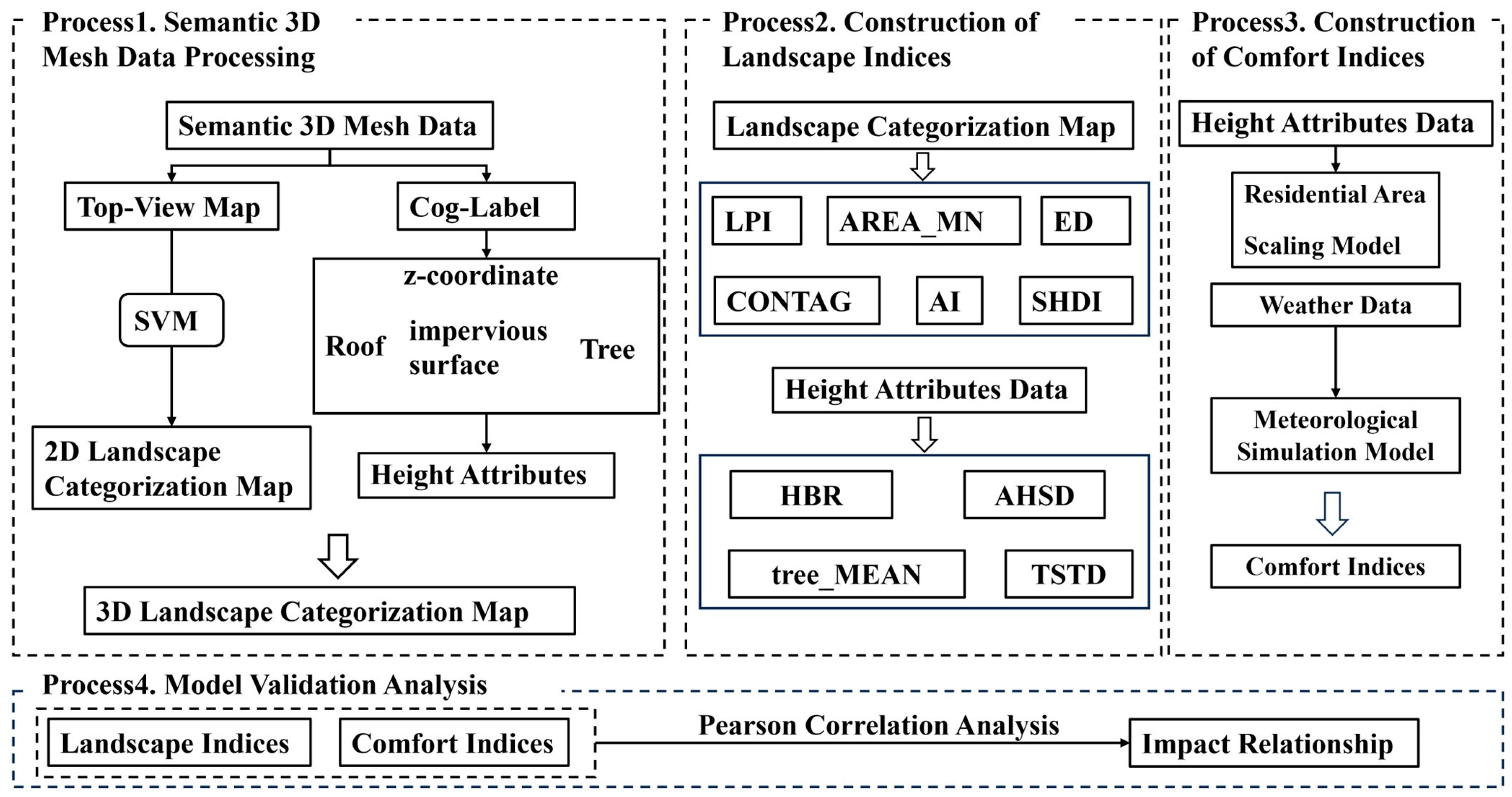
Furthermore, this study achieves precise quantification of ground, building, and tree heights within the study area by leveraging the centroid labels obtained from three-dimensional mesh semantic segmentation and their corresponding z-coordinates. A height index system is subsequently constructed. The specific steps are as follows: For ground height calculation, the z-coordinates of centroid points from segmented patches are extracted, and statistical analysis is applied to estimate the ground height for each tile unit, providing a reference plane for subsequent height calculations. Building heights are accurately derived by computing the vertical distance between the ground height and the z-coordinates of roof patch centroids. Similarly, tree heights are determined by comparing the ground height with the z-coordinates of tree patch centroids. These height data form the basis for constructing building and tree height indices (

Table 4. The building and tree height indices.

Region Name	HBR	BHSD	ATH	THSD
Region 1	0.3711	41.4979	4.0819	2.5008
Region 2	0.8923	9.2943	3.6290	2.4263
Region 3	0.7961	10.6767	4.6457	3.3673
Region 4	0.6489	10.5181	5.0550	3.2695
Region 5	0.4864	42.0021	4.9329	3.1821
Region 6	0.8502	13.6099	4.2134	2.8096
Region 7	0.9663	6.3671	3.3265	2.8644
Region 8	0.6349	29.5854	4.2781	2.9860
Region 9	0.9695	6.6690	3.2566	3.6281

).

The data presented in Table 4 reveal significant spatial heterogeneity in the distribution of building heights and tree heights across the study areas.

In terms of building height characteristics, the high-rise building ratio reflects the proportion of tall buildings within each region. Regions 7 and 9 exhibit the highest ratios among all study areas, indicating a denser concentration of high-rise buildings in these zones. Meanwhile, the standard deviation of building heights measures the variability in building heights within each region. Regions 1 and 5 display the largest standard deviations, suggesting pronounced disparities in building heights, which may stem from diverse urban planning strategies or phased construction timelines. This variability underscores the complexity of spatial morphology in these areas.

Regarding tree height characteristics, region 4 stands out with an average tree height of 5.055 m and a standard deviation of 3.2695, indicating not only a relatively high vegetation cover but also notable variability in tree heights. This variability likely reflects a mix of tree species and age classes. In contrast, regions 9 and 7 exhibit similar average tree heights (3.3265 m and 3.2566 m, respectively), with a modest difference in their standard deviations (0.7637). This suggests that while the average tree heights in these regions are comparable, region 7 exhibits a slightly more dispersed vertical structure, resulting in a more layered canopy profile.

3.4. Result of Comfort Index of Residential Area

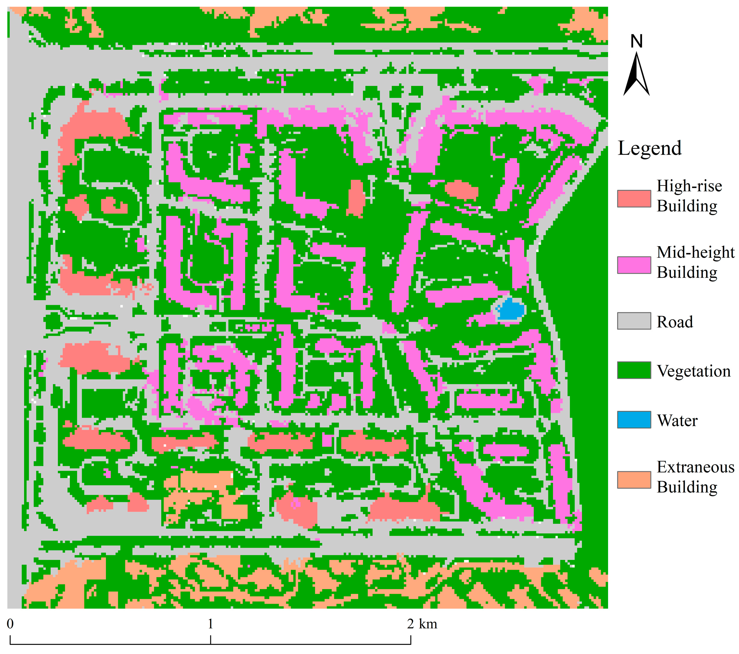
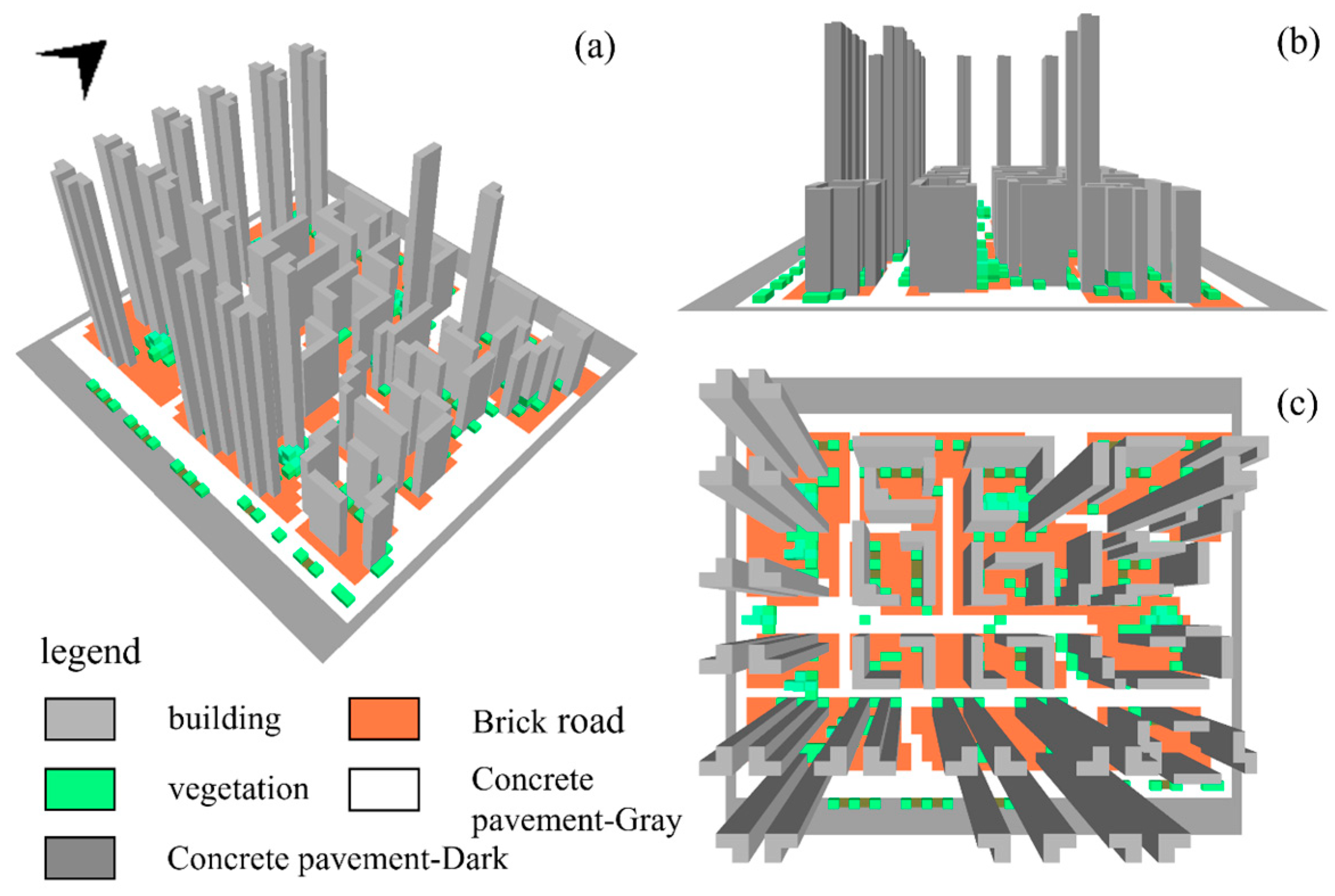
Before conducting simulations using the 3D nonhydrostatic fluid model, this study constructed a residential area model suitable for meteorological simulation models based on the top view of 3D grid data (Figure 7). The material settings for buildings and vegetation in the model are as follows: The material of the buildings is set as medium-insulating walls with layer thicknesses of 0.01 m, 0.12 m, and 0.18 m, and a roughness length of 0.02 m. There are two types of vegetation involved: one is shrubs with heights between 1 m and 2 m; the other is cylindrical in structure, with small trunks, dense growth, and a height of approximately 5 m, used to simulate the trees in the residential area. Secondly, upon completing the construction of the three-dimensional spatial model of the residential area, this study coupled it with a meteorological model to achieve precise simulation of residential comfort under varying seasonal weather conditions. The specific steps are as follows: The constructed three-dimensional spatial model of the residential area was imported into professional meteorological simulation software. The meteorological simulation parameters mainly include the start and end times of the simulation, initial meteorological data, soil parameters, and building temperature parameters. The start times set in this study are 5:00 a.m. on 21 July 2024 and 5:00 a.m. on 26 January 2024, with a simulation duration of 18 h for each. The initial weather conditions include the average temperature, wind speed and direction, and relative humidity over the past 12 h. The average temperature and relative humidity are based on data measured by the meteorological station. The wind speed is set to be constant at 2.00 m per second at the inflow boundary at a height of 10 m. The wind direction is also set to be constant at 90.00 degrees at the inflow boundary at a height of 10 m, indicating that the wind is blowing from the due east. The soil parameters are set as follows: The upper soil layer (0–20 cm) has a soil temperature of 20.00 °C. The middle soil layer (20–50 cm) also has a soil temperature of 20.00 °C. The deep soil layer (50–200 cm) has a soil temperature of 19.00 °C. The bedrock layer soil (below 200 cm) has a soil temperature of 18.00 °C. The building temperature parameters are set as follows: The indoor building temperature is 20.00 °C, which is the initial temperature inside the building. The initial building surface temperature is also set at 20.00 °C, which refers to the temperature of the building surface at the start of the simulation. Moreover, it is chosen that the temperature inside the building will be influenced by the external microclimate and will not remain constant.

Based on meteorological data from Wuhan on 26 January 2024 and 21 July were selected as typical winter and summer meteorological days for simulation, respectively. These dates represent the characteristic climatic features of the local winter and summer seasons, and simulating these two dates effectively captures the impact of seasonal variations on the thermal environment of the residential area.

During the meteorological simulation process, to comprehensively evaluate residential comfort at different spatial heights, this study scientifically divided the height levels. Referencing the standard height for pedestrian perception of air temperature, a model height of 1 m was equated to an actual height of 1.6 m, serving as the baseline height for pedestrian activity layers. The spatial height was further divided into three levels: low, medium, and high. The low-level range spanned from a model height of 1.4 m to 5 m (corresponding to actual heights of 2.24 m to 8 m), primarily encompassing pedestrian activity areas and spaces with low-lying vegetation. The medium level ranged from a model height of 7 m to 17 m (actual heights of 11.2 m to 27.2 m), covering most mid-rise buildings and intermediate vegetation zones. The high level extended from a model height of 19 m to 49 m (actual heights of 30.4 m to 78.4 m), mainly involving the tops of high-rise buildings and canopy layers of trees.

To investigate the variation patterns of residential comfort under different climatic conditions, this study selected meteorological data from distinct seasons for comparative analysis. For summer, meteorological data from 14:00 on 21 July 2024, were used as an example, while for winter, data from 14:00 on 26 January 2024, were employed. The study obtained key meteorological parameters across different height levels, including mean air temperature, relative humidity, temperature-humidity index, and PMV index, as detailed in

Table 5. Average value of meteorological simulation data for residential areas on 21 July 2024.

Height Classes	Pedestrian Height	Low	Medium	High
Average Temperature (°C)	37.7074	37.5684	36.6258	35.7493
Average RH (%)	44.0136	44.3850	45.3332	45.4105
Average THI	31.4588	30.4817	29.9430	29.3395
Average PMV	4.9977	4.9520	4.8259	4.6329

and

Table 6. Average value of meteorological simulation data for residential areas on 26 January 2024.

Height Classes	Pedestrian Height	Low	Medium	High
Average Temperature (°C)	8.0535	7.7147	6.6960	5.9149
Average RH (%)	51.2979	53.2377	62.8252	73.3664
Average THI	9.7535	9.4308	8.2683	7.1492
Average PMV	−3.0587	−3.1481	−3.2310	−3.2023

.

According to Table 5, the thermal environment parameters of the study area exhibit significant vertical stratification characteristics during summer. Specifically, in terms of air temperature distribution, the average temperature at the pedestrian activity level (1.6 m height) reaches the daily peak, while temperatures decrease with increasing vertical height. The relative humidity remains relatively stable across all height levels, with a mean value of approximately 44%. This result indicates that, during high temperature periods in summer, the vertical distribution of water vapor in the study area is minimally influenced by factors such as building layout and vegetation coverage, exhibiting a homogenized pattern overall.

The analysis of the THI reveals that the highest THI value occurs at the pedestrian activity level (31.4588), while the lowest is observed in the high-rise zone (29.3395). Based on the human comfort classification standard (where THI > 27.5 indicates a muggy and uncomfortable range), the average THI values across all height layers in the study area significantly exceed the threshold, indicating that the overall thermal environment exceeds the tolerable comfort range for humans. Notably, the low-rise zone (2.24–8 m), characterized by high building density and limited ventilation, exacerbates the muggy sensation due to ground radiation and metabolic heat production, posing a significant challenge to the thermal comfort of residents and pedestrians.

From the perspective of the PMV assessment, the PMV values for all height levels exceed 4, significantly deviating from the ASHRAE thermal comfort standard (−0.5 to 0.5). This result suggests that residents across different floors generally exhibit low subjective satisfaction with the summer thermal environment. Moreover, the PMV values increase as height decreases, further corroborating the conclusion of deteriorating thermal comfort in low-rise areas.

According to Table 6, the variation pattern of residential comfort in winter is similar to that in summer. In terms of air temperature, the temperature decreases with increasing floor height in both seasons, but the lowest temperature in the high-rise zone (>30.4 m) during winter is 5.9149 °C, while the temperature at the pedestrian activity level (1.6 m) reaches 8 °C, indicating a more pronounced temperature gradient compared to summer.

Regarding relative humidity, the overall level in winter is significantly higher than in summer, and it exhibits an increasing trend with height. The difference in relative humidity between the mid-rise (11.2–27.2 m) and high-rise (30.4–78.4 m) zones reaches 10%. Based on the human settlement comfort classification standard (where a temperature-humidity index, THI < 14, indicates extreme cold conditions), the THI values across all height layers in the study area are significantly below the threshold, indicating that the overall thermal environment in winter is in a state of cold discomfort.

Unlike the summer pattern, where the pedestrian level exhibited the highest THI values, the pedestrian activity level in winter, despite having a relatively higher THI (9.8765), remains within the cold range. Meanwhile, the high-rise zone has a THI of only 7.1492, reflecting a more intense perception of cold among residents in this area.

In terms of the PMV, the comfort levels vary significantly across different height layers. The pedestrian activity level has the highest PMV value, while the mid-rise zone has the lowest. The difference in PMV values between the high-rise and mid-rise zones is relatively small. Combined with the THI analysis, the high-rise zone, due to the combined effects of low temperature and high humidity, experiences a significant decline in thermal comfort, making it the area with the poorest thermal comfort conditions during winter.

3.5. Extraction of the Residential Area Comfort Zonal Index

The Residential Area Comfort Zonal Index (RACZI) exhibits unique advantages over the Residential Area Comfort Overall Index (RACOI) in assessing the quality of human settlements. While the overall index reflects the average comfort level of the entire residential area from a macro perspective, it struggles to capture the spatial heterogeneity within the area. In contrast, the RACZI focuses on localized spatial units, enabling a more refined and differentiated analysis of environmental characteristics. Building upon the meteorological simulation data for summer and winter, this study further extracts the Residential Area Comfort Index (RACI) for each subzone (

Table 7. Partitioned air temperature data of residential area in summer.

Region Name	APLAT	ALRAT	AMRAT	AHRAT	Average
Region 1	37.6114	37.5532	37.0218	36.0628	37.0623
Region 2	37.7127	37.6720	37.2025	36.0663	37.1634
Region 3	37.9489	37.8883	37.3256	36.0239	37.2967
Region 4	37.6051	37.4743	36.6613	35.6780	36.8547
Region 5	37.5978	37.5209	36.9028	35.9990	37.0051
Region 6	37.3815	37.3532	36.9913	35.9093	36.9088
Region 7	37.6281	37.5233	36.7455	35.6501	36.8867
Region 8	37.3338	37.2724	36.6815	35.8302	36.7795
Region 9	37.2970	37.1519	36.3129	35.5426	36.5761

Here, APLAT represents the average air temperature at pedestrian height, ALRAT denotes the average air temperature in low-rise building zones, AMRAT stands for the average air temperature in mid-rise building zones, and AHRAT indicates the average air temperature in high-rise building zones.

and

Table 8. Partitioned air temperature data of residential area in winter.

Region Name	APLAT	ALRAT	AMRAT	AHRAT	Average
Region 1	7.3783	7.3110	6.9036	6.1369	6.9325
Region 2	8.5304	7.4838	7.1408	6.1267	7.3204
Region 3	7.5264	7.7185	7.2957	6.1188	7.1649
Region 4	7.8634	7.4429	6.6841	5.8035	6.9485
Region 5	8.5190	8.3356	7.3652	6.3357	7.6389
Region 6	7.7878	7.7462	7.1017	5.9860	7.1554
Region 7	7.6873	7.4972	6.7335	5.7569	6.9187
Region 8	7.7240	8.2430	7.0912	6.1370	7.2988
Region 9	7.8582	7.4864	6.4670	5.6742	6.8715

Here, APLAT represents the average air temperature at pedestrian height, ALRAT denotes the average air temperature in low-rise building zones, AMRAT stands for the average air temperature in mid-rise building zones, and AHRAT indicates the average air temperature in high-rise building zones.

) to analyze the impact of residential building density on comfort levels.

According to Table 7, there are significant horizontal variations in air temperature across different regions. In summer, region 3 exhibits the highest average temperature across all height levels, followed by region 2. Region 3 is located in the upper-middle right part of the residential area, characterized by high building density and compact layouts, which hinder air circulation and create a typical heat island effect. In contrast, region 9 records the lowest average temperature at the mid-rise building height level, while region 8 has the lowest average temperature in the high-rise building zone. These two regions benefit from lower building density, higher green coverage, and surrounding open spaces that facilitate air convection, effectively mitigating summer heat. This indicates that the lower-right area of the residential zone exhibits superior thermal environmental conditions during summer, offering higher livability.

According to the data in Table 8, the average air temperature in Zone 5 at the pedestrian activity level is significantly higher than in other zones. This zone is located in the upper-middle part of the residential area, with a high building density. The dense building clusters form a relatively enclosed space, effectively reducing heat dissipation. In contrast, the pedestrian-level temperatures in other zones are all below 8 °C. At the low-rise level, Zone 1 exhibits the lowest average temperature, while Zone 5 has the highest. In the mid-rise level, Zone 9, located in the lower-right corner of the residential area, has the lowest average temperature, primarily due to the larger building spacing and lack of effective shading, leading to rapid heat dissipation. Further analysis of the average temperatures across all height levels reveals that Zone 1 in the upper-left corner and Zone 9 in the lower-right corner of the residential area have the lowest temperatures, making these zones the coldest during winter. Conversely, Zones 2 and 5 exhibit significantly higher average temperatures than other zones, indicating better thermal insulation performance in winter.

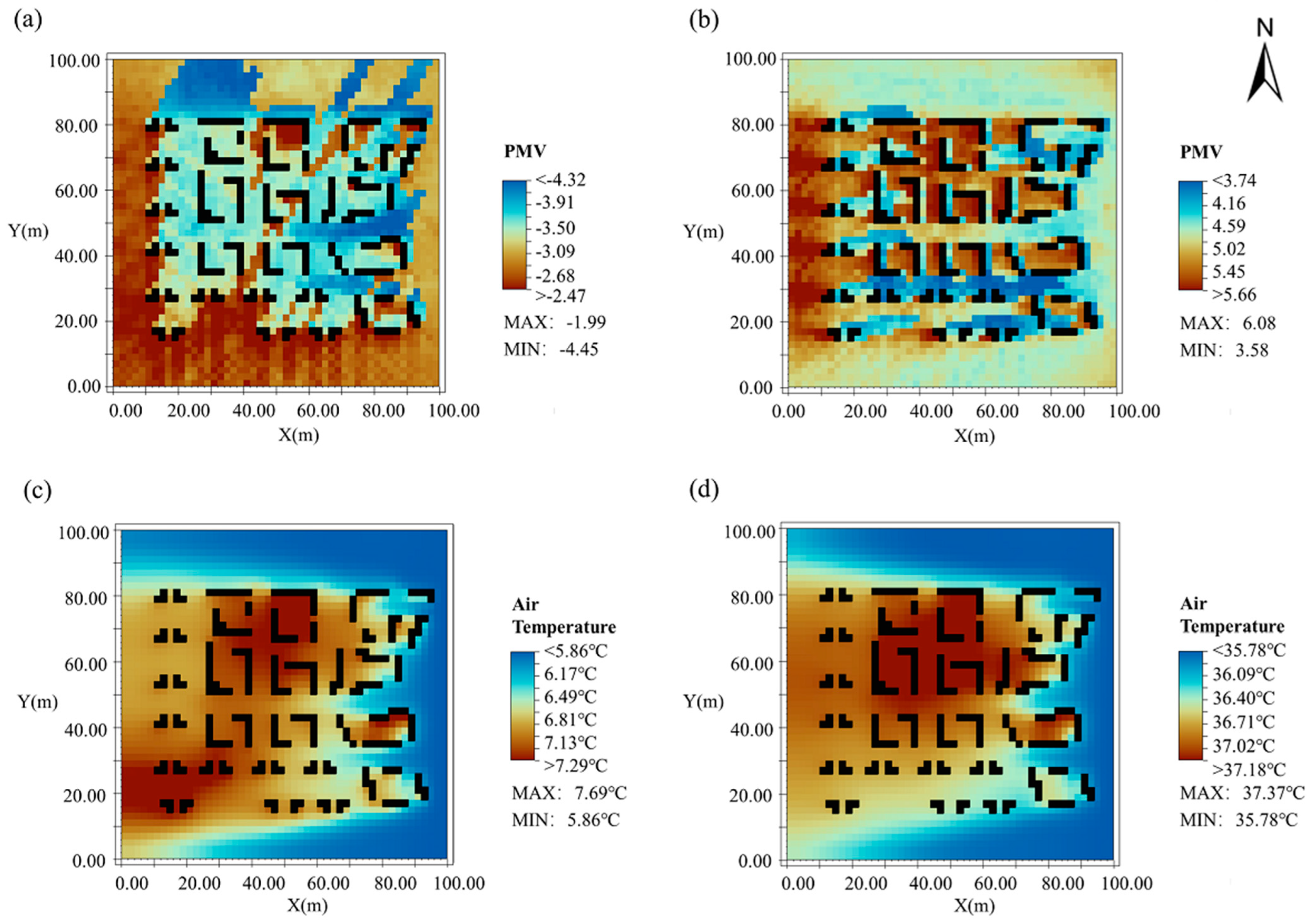
PMV is a crucial indicator for assessing human thermal comfort, directly reflecting residents’ thermal perceptions in different zones. This study is based on data from two days in winter and summer 2024 at 14:00 and a model height of 15 m. The PMV index is visualized alongside temperature indicators for winter and summer (Figure 8) to further reveal the spatiotemporal variations of PMV and its coupling relationship with the thermal environment. Figure 8 shows significant spatial differences in PMV values between winter and summer. In winter, Zones 3, 8, and 9 exhibit relatively high PMV indices, approaching 0, indicating that residents in these zones experience relatively comfortable thermal conditions. In summer, Zones 2, 3, 6, and 7 display extensive brown areas (high PMV values), with PMV indices significantly deviating from the comfort range, suggesting widespread discomfort due to heat and humidity. This aligns closely with the high temperature distribution in these zones: summer high temperature areas are concentrated in Zones 2, 3, and the southwestern part of Zone 4, primarily influenced by the heat island effect of high-density building clusters. The high temperature trend in the central part of Zone 7 is closely related to compact building layouts and poor ventilation. Comparing the temperature distribution characteristics between winter and summer, the high temperature zones in winter are mainly distributed in the southern part of Zone 5, the western part of Zone 6, and the northeastern parts of Zones 2 and 3. This phenomenon may be attributed to the interception of solar radiation by building orientation and layout morphology.

3.6. Correlation Analysis Between Landscape Index and Residential Area Comfort Index

Landscape indices, as essential tools for quantifying landscape pattern characteristics, exhibit complex and significant relationships with residential comfort indicators. This study selected five categories of landscape indices—area and edge metrics, aggregation metrics, diversity metrics, building metrics, and tree metrics—to construct a dual-dimensional landscape index system, investigating the influence of landscape patterns on residential comfort during winter and summer. Among these, area and edge metrics, aggregation metrics, and shape metrics integrate three-dimensional classification information, focusing on the spatial morphological features of the landscape. In contrast, building metrics and tree metrics are derived from height data, reflecting the vertical structural attributes of the landscape.

The Pearson correlation analysis method was employed to examine the relationships between the selected landscape indices and comfort indicators. To ensure spatial scale consistency, the study area, initially divided into 50 × 50 grids, was resampled to 10 × 10 grids to match the spatial resolution of the landscape index tiles. Subsequently, the landscape index values for each region were integrated with the corresponding comfort indicators (air temperature, relative humidity, temperature-humidity index, and PMV index) to construct a standardized dataset. The Pearson correlation coefficient matrix was calculated to visualize the correlation characteristics between landscape indices and comfort indicators, with heatmaps (Figure 9, Figure 10, Figure 11 and Figure 12) providing an intuitive representation.

The labels for comfort indicators in the heatmaps are defined as follows:

• APLAT: Average Pedestrian Level Air Temperature
• ALRAT: Average Low-Rise Air Temperature
• AMRAT: Average Mid-Rise Air Temperature
• AHRAT: Average High-Rise Air Temperature
• APLRH: Average Pedestrian Level Relative Humidity
• ALRRH: Average Low-Rise Relative Humidity
• AMRRH: Average Mid-Rise Relative Humidity
• AHRRH: Average High-Rise Relative Humidity
• APLTHI: Average Pedestrian Level Temperature-Humidity Index
• ALRTHI: Average Low-Rise Temperature-Humidity Index
• AMRTHI: Average Mid-Rise Temperature-Humidity Index
• AHRTHI: Average High-Rise Temperature-Humidity Index
• APLPMV: Average Pedestrian Level Predicted Mean Vote
• ALRPMV: Average Low-Rise Predicted Mean Vote
• AMRPMV: Average Mid-Rise Predicted Mean Vote
• AHRPMV: Average High-Rise Predicted Mean Vote

This analysis elucidates the spatial and temporal heterogeneity of landscape effects on residential comfort, providing a foundation for optimizing urban design and improving thermal environments in residential areas.

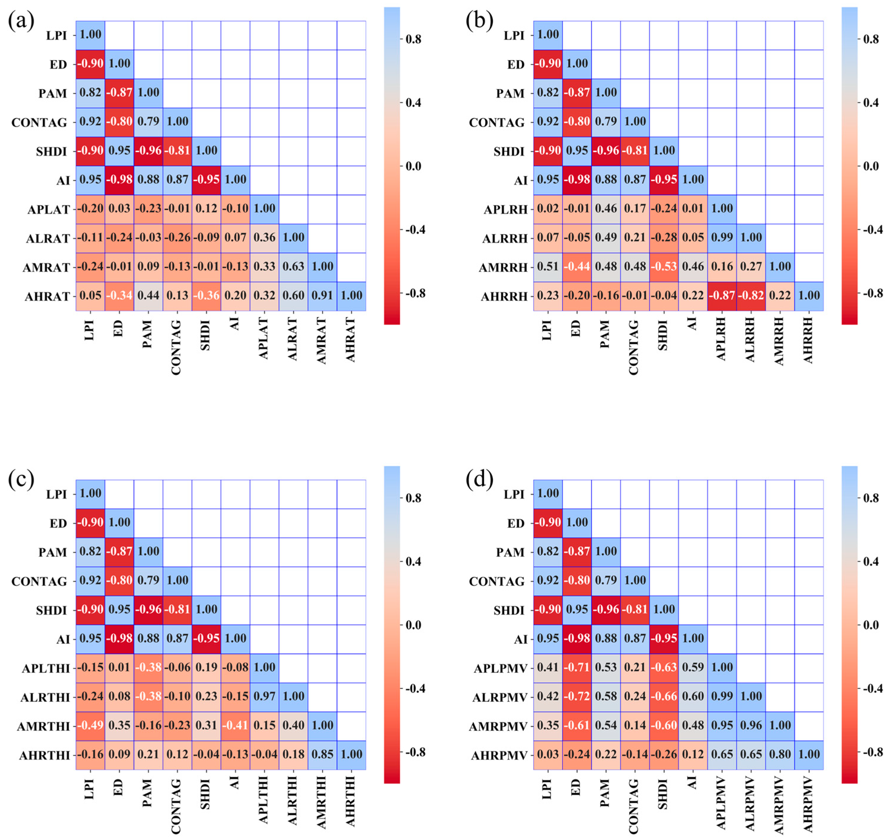
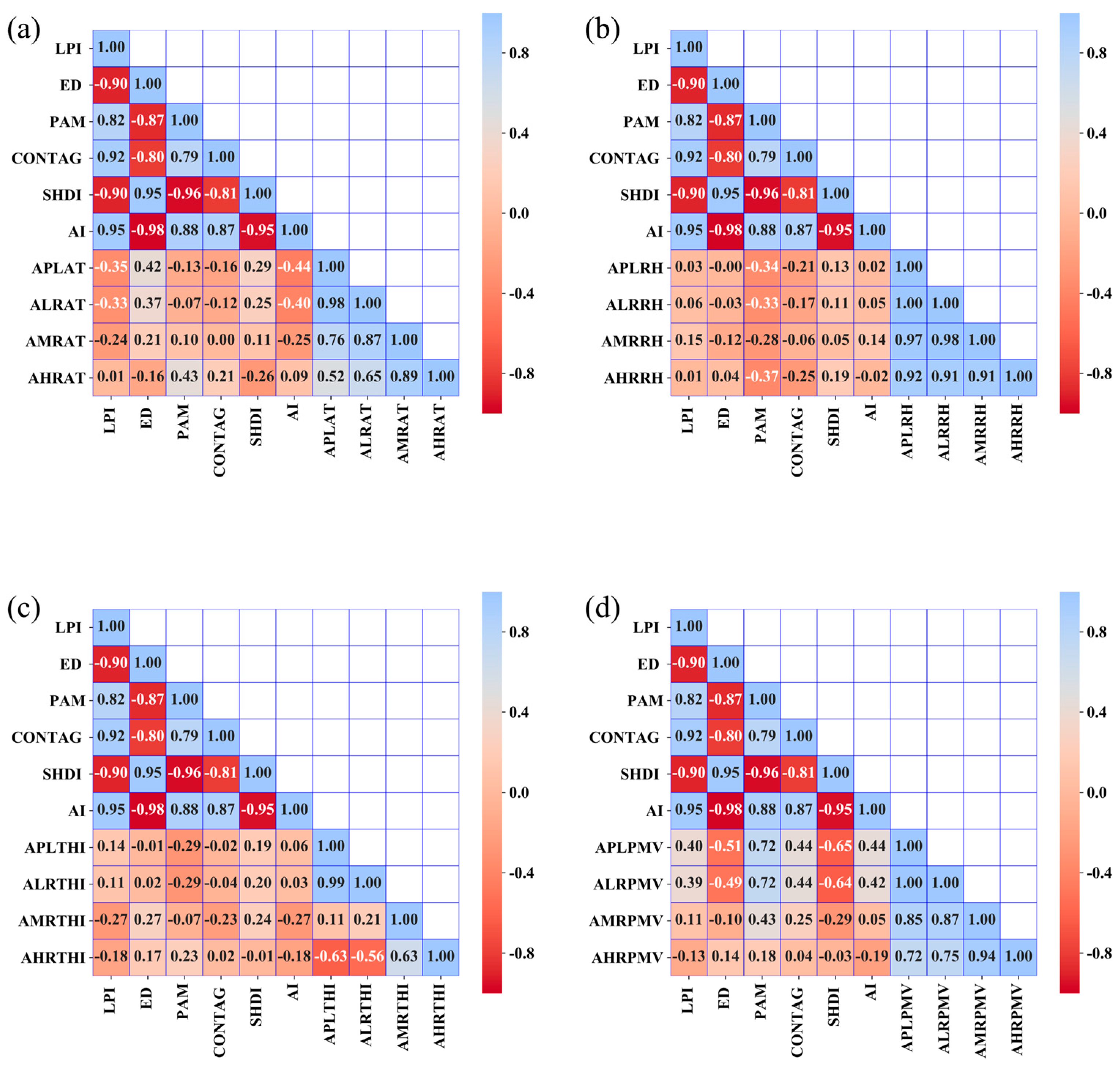
According to Figure 9, the correlation between the winter LPI and comfort indicators exhibits significant vertical stratification differences. Regarding relative humidity, the correlation coefficient between LPI and AMRRH is 0.51, indicating a moderate positive relationship. This suggests that an increase in the scale of dominant patches contributes to higher air humidity in mid-rise areas. In contrast, the correlation between LPI and APLRH is the weakest, approaching 0.02, reflecting a negligible influence of this index on near-ground humidity. The dominant patches in the residential area are vegetation, which indicates that an increase in vegetation area in the residential area leads to a rise in air humidity in the mid-level regions, while the air humidity at the pedestrian activity level is not significantly related to whether the vegetation area is dominant. To address the issue of relatively high humidity at medium heights causing a cold and damp feeling, it can be achieved by reducing the excessive density of vegetation around buildings. ED demonstrates a pronounced negative relationship with thermal comfort indicators. ED shows strong negative correlations with the ALRPMV, AMRPMV, and APLPMV, indicating that increased landscape edge complexity significantly reduces residents’ thermal comfort. Conversely, ED exhibits an extremely weak correlation with APLRH, suggesting its limited role in humidity regulation. This indicates that fragmented landscapes are not conducive to keeping warm in the lower floors, mid-level floors, and pedestrian activity layers of residential areas during winter. The more fragmented the overall landscape is, that is, the more sparsely green spaces are divided by buildings, the more likely it is to cause a cold sensation in winter. However, the degree of landscape fragmentation has little impact on relative humidity.

The PAM displays spatial heterogeneity in its correlation with temperature indicators. Vertically, PAM is negatively correlated with the average air temperature of low-rise and pedestrian layers but positively correlated with mid- and high-rise temperatures, revealing divergent mechanisms of influence on thermal environments across different height layers The PAM reflects the evenness of landscape patches, which indicates that an even distribution of green spaces and vegetation in residential areas is beneficial for reducing the sensation of coldness on mid-level floors during winter. CONTAG generally exhibits weak correlations with PMV indicators. The correlation coefficients between PMV and CONTAG across all height layers are below 0.4, with a notably weak negative correlation for high-rise PMV, suggesting that improved connectivity of dominant patches has limited effects on enhancing thermal comfort in high-rise areas, which means that the connectivity of vegetation does not have an impact on the thermal comfort of high-rise buildings. The SHDI shows no significant relationship with temperature indicators. Vertically, the correlation coefficients between SHDI and the average temperatures of pedestrian, low-rise, mid-rise, and high-rise layers are 0.12, −0.09, −0.01, and −0.36, respectively, without a clear pattern. This implies that landscape diversity, including the diversity of building types and vegetation within the residential area, exerts a complex influence on winter thermal environments. The AI demonstrates strong environmental regulation effects in mid-rise areas. AI exhibits moderate correlations with the average PMV, average temperature-humidity index, and average relative humidity in mid-rise regions, indicating that increased clustering of similar landscape patches, such as the aggregated distribution of buildings and aggregated distribution of green spaces, can effectively improve the thermal and humidity conditions of mid-rise spaces.

As shown in Figure 10, the correlation between the summer LPI and air temperature across different heights is similar to that observed in winter. However, its humidity regulation effects exhibit seasonal variations. Unlike the moderate positive correlation with mid-level relative humidity in winter, LPI shows only weak positive correlations with relative humidity at all height levels in summer, indicating a significantly reduced influence of dominant landscape patches on humidity enhancement during summer. In terms of temperature response, LPI exhibits consistent positive correlations with air temperature across all height levels in both seasons, confirming its seasonally stable warming effect on the thermal environment.

The ED displays negative correlations with summer comfort indicators. Except for high-rise PMV, the absolute correlation coefficients between ED and PMV at pedestrian and low-rise levels approach 0.5, indicating moderate negative correlations—weaker than the strong negative correlations observed in winter. This suggests that increased landscape edge complexity exacerbates thermal discomfort near the ground in summer but has a limited impact on high-rise thermal conditions. An increase in edge density will expand the heat exchange area between high temperature surfaces and the air, forming a source of thermal radiation, which can easily exacerbate thermal discomfort. PAM shows significantly enhanced associations with summer comfort indicators. It exhibits strong positive correlations with PMV at low-rise and pedestrian levels and moderate positive correlations with mid-rise PMV, highlighting the beneficial role of large vegetation landscape patches in improving thermal comfort during summer. CONTAG undergoes notable seasonal shifts in its correlations with summer thermal indicators. Its positive correlations with PMV across all height levels strengthen compared to winter, while its correlations with relative humidity shift from uniformly positive in winter to uniformly negative in summer. This reversal suggests that dominant landscape connectivity may reduce air humidity by accelerating moisture diffusion while simultaneously improving thermal comfort in summer. SHDI exhibits a seasonal reversal in its correlations with relative humidity. In summer, SHDI transitions from negative to positive correlations with relative humidity at all height levels, indicating its regulatory role in humidity during this season. Conversely, AI shows significantly reduced correlations with summer thermal-humidity indices. The correlation coefficient for mid-rise thermal-humidity indices drops from 0.41 in winter to 0.27, while the low-rise coefficient declines from 0.15 to 0.03, reflecting diminished effectiveness of homogeneous landscape aggregation in improving summer thermal-humidity conditions. The aggregated distribution of vegetation and buildings is not conducive to the improvement of humidity and heat in buildings during summer.

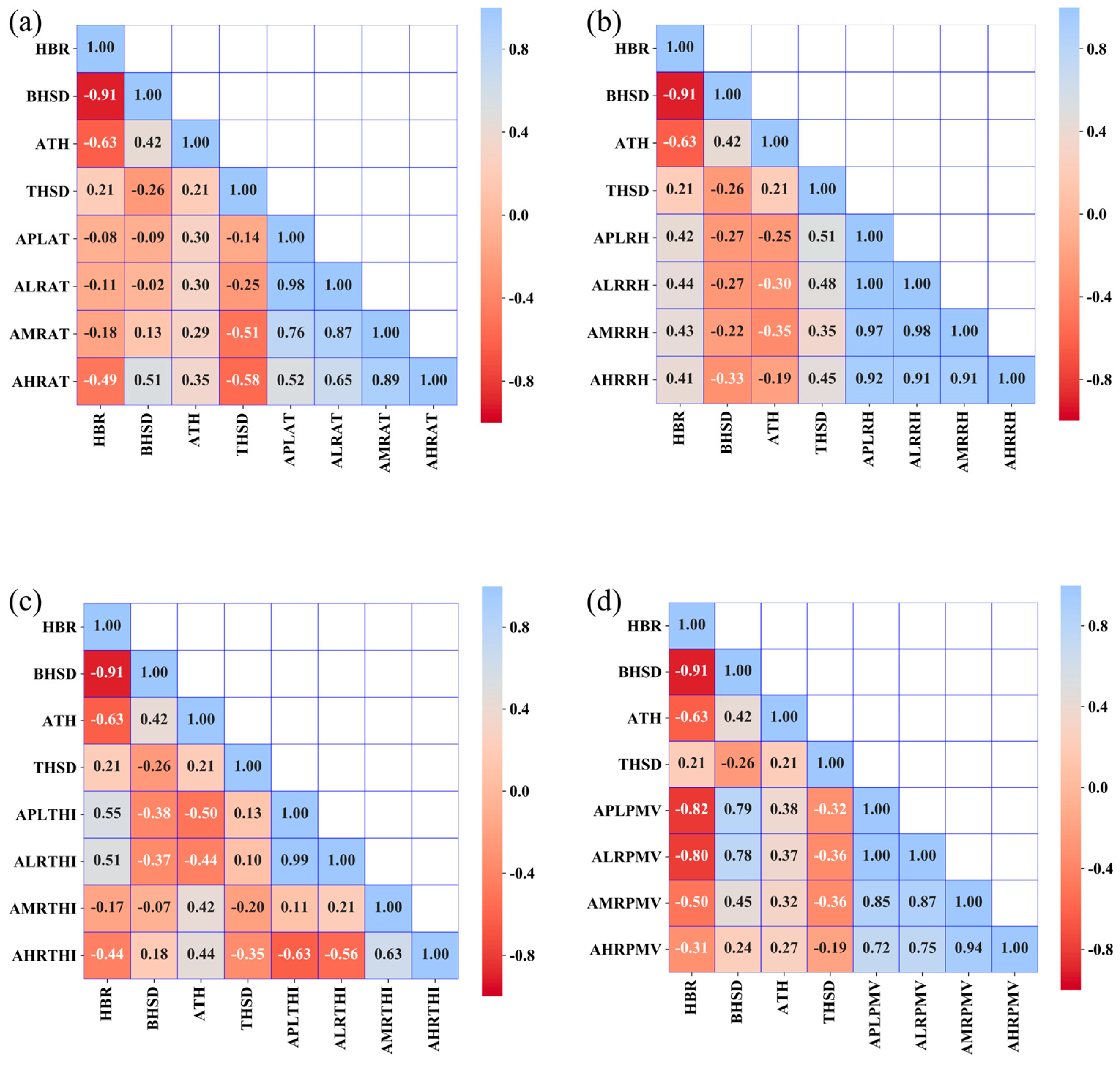
As shown in Figure 11, in terms of air temperature response, the standard deviation of building height and the average tree height exhibit moderate positive correlations with air temperature at low and middle floors (r > 0.4), indicating that increased variability in building height and elevated tree height significantly intensify thermal effects at these levels. However, the correlation between air temperature at pedestrian level and these indices is weak (r < 0.1), suggesting that near-ground thermal conditions are primarily influenced by other localized factors. The high building ratio index shows negative correlations with air temperature across all heights except pedestrian level, with a particularly strong negative correlation at high floors (r ≈ −0.7), implying that densely clustered high-rise buildings in winter tend to form cold island effects, exacerbating heat dissipation at upper levels.

The relationship between relative humidity and building/tree indices displays notable spatial heterogeneity, with the same index exhibiting divergent effects on humidity across different height layers. Regarding THI, the average tree height demonstrates the strongest correlation with THI at middle floors (r = 0.52), highlighting the significant regulatory role of vertical tree distribution on the combined thermal and humidity conditions in these zones. The high building ratio exhibits weak correlations with THI across all heights (absolute r values ranging from 0.2 to 0.4). Additionally, the moderate correlation between the standard deviation of tree height and humidity at high floors further corroborates the influence of vegetation vertical structure on the thermal-humidity environment in elevated areas.

For the PMV index, the standard deviation of building height shows extremely strong correlations (r > 0.8) with PMV at pedestrian, low, and middle floors, underscoring the substantial impact of building height variability on thermal comfort near the ground and at intermediate levels. The high building ratio is negatively correlated with PMV across all floors, with particularly strong negative correlations at low and middle floors (r ≈ −0.6), revealing that high-density high-rise areas in winter are prone to exacerbating residents’ cold sensations.

Figure 12 reveals significant seasonal variations in the correlation between building/tree indices and air temperature during summer compared to winter. Specifically, except for the standard deviation of tree height, the correlation coefficients between height-related indices and high-rise air temperature exhibit a notable decline in summer. The absolute values of correlation coefficients for building height standard deviation, HBR, and average tree height decrease from 0.64, 0.73, and 0.50 in winter to 0.49, 0.51, and 0.35 in summer, respectively. This suggests that the influence of high-rise building density and tree height on summer thermal conditions weakens compared to winter.

The correlation between relative humidity and height-related indices also undergoes significant seasonal shifts. The HBR shows the most pronounced change, transitioning from negative to positive correlations across most height levels, except for high-rise humidity. Similarly, the building height standard deviation shifts from positive to negative correlations, indicating a more complex relationship between summer humidity distribution and building height patterns, likely influenced by localized microclimates.

Notably, the correlation between HBR and the THI strengthens in summer, particularly at low-rise and pedestrian levels, where it rises from weak to moderate. The building height standard deviation also shows enhanced correlations with THI at pedestrian and low-rise heights, with coefficients increasing from 0.12 and 0.09 to 0.38 and 0.37, respectively. This highlights the heightened impact of building height distribution on summer thermal-humidity conditions, especially in lower elevations.

Furthermore, the standard deviation of tree height transitions from very weak to weak negative correlations with summer PMV, indicating a slightly stronger influence of trees on thermal comfort. Meanwhile, the HBR exhibits a dramatic increase in correlation with PMV at pedestrian and low-rise levels, reaching absolute values of approximately 0.8, underscoring its dominant role in shaping microclimates in high-density building areas. These findings collectively emphasize the critical role of building morphology in regulating summer thermal environments, particularly in densely built zones.

4. Discussion

Residential comfort is not only a core indicator of quality of life, directly influencing individual well-being, but also a critical factor in achieving global energy-saving and emission-reduction goals [55]. By analyzing the spatial distribution of green spaces and buildings in residential areas, this study elucidates the relationship between landscape patterns and resident comfort, providing a theoretical foundation for optimizing temperature regulation mechanisms, reducing energy consumption, and enhancing livability. Focusing on the spatial characteristics of green and built-up landscapes, this research quantitatively examines their two-dimensional (2D) and three-dimensional (3D) structures, systematically revealing their impact on thermal comfort. The findings demonstrate that, under identical meteorological conditions, residents’ thermal experiences are closely linked to floor height, building density, and the size and vertical distribution of nearby green spaces.

The study introduces an integrated 2D–3D landscape assessment framework to analyze regional variations in landscape features and their spatial influences. The inclusion of 3D metrics significantly alters the quantification of landscape indices, particularly aggregation and diversity indices, which more accurately reflect vertical elements such as building height and vegetation structure. Area- and edge-related metrics exhibit pronounced disparities across zones, with the LPI highlighting uneven distributions of dominant patches (e.g., vegetation or buildings). For instance, Zone 1 has the highest LPI, indicating low fragmentation, while Zone 3, with the smallest dominant patches, shows high fragmentation. The ED further corroborates this, with Zones 3 and 4 displaying fragmented landscapes and poor connectivity, whereas Zones 5 and 8 feature continuous green spaces and cohesive ecological structures. The AI reveals strong spatial continuity in most zones, except Zone 3, where fragmentation reduces connectivity. Zones 2, 6, and 9 exhibit similar AI values, suggesting analogous spatial configurations of green and built-up areas.

3D height metrics uncover additional vertical disparities. The HBR indicates dense high-rises in Zones 8 and 9, contrasting with varied heights in Zones 1 and 5, which influence microclimate and heat dissipation. Tree height analysis shows Zone 7 dominated by uniformly low vegetation, while Zones 4 and 5 feature taller, vertically diverse but spatially limited trees. These structural differences affect both ecological functionality and thermal comfort. Seasonal analyses of comfort metrics reveal that air temperature decreases with height year-round, while relative humidity varies significantly between seasons. The THI shows summer comfort improves at higher floors, whereas the PMV indicates the worst summer discomfort at pedestrian levels and winter cold stress in high-rises. Spatially, summer hotspots concentrate in Zones 1–3, with cooler areas in Zones 8–9, while winter temperatures are more heterogeneous, peaking in Zones 2, 5, and 8 and dropping sharply in Zones 7 and 9.

The type and layout of vegetation play a crucial role in influencing thermal comfort in residential areas. Studies have shown that different vegetation configurations can significantly impact the microclimate and human thermal comfort. For example, a combination of trees, shrubs, and grass provides the best thermal comfort compared to other configurations. The density and arrangement of vegetation also matter. Uniformly distributed trees and grass offer the most effective cooling and humidifying effects, especially in summer. In contrast, dense planting arrangements can enhance wind circulation and reduce local temperatures more effectively. In addition, the choice of vegetation type is important. Evergreen conifers and broad-leaved trees with large, hairy, or sticky leaves are particularly effective in absorbing fine particulate matter and improving air quality, which indirectly contributes to thermal comfort. For instance, mature trees can significantly filter pollutants, enhancing the overall environmental quality of residential areas [56].

Pearson correlation analyses quantify relationships between landscape indices and comfort metrics, highlighting multi-layered influences. The PAM correlates negatively with air temperature and THI but positively with PMV, suggesting smaller, evenly distributed patches enhance pedestrian comfort. HBR exhibits seasonal duality: winter negative correlations with humidity and PMV and summer positive links with THI, implicating high-rise clusters in thermal discomfort. AI strongly correlates with low-floor PMV, improving winter insulation but exacerbating summer heat. Building height uniformity benefits year-round comfort, while LPI’s winter negative correlation with mid-floor THI underscores dominant patches’ role in cold dampness. Tree height uniformity critically affects summer mid-floor cooling and year-round high-rise comfort, with Shannon diversity reducing winter high-rise temperatures. Notably, 3D-integrated indices show weaker high-floor correlations, emphasizing the need for tailored metrics. These insights advocate for stratified landscape planning to optimize thermal comfort across all residential zones.

5. Conclusions

This study adopts a residential area in Wuhan as the horizontal scale and building height as the vertical scale, constructing two-dimensional and three-dimensional landscape indices from both horizontal and vertical analytical dimensions. By simulating meteorological data of the residential area using a climate model, the study systematically explores the intrinsic relationship between the spatial patterns of buildings and green spaces and residential comfort. The following conclusions are drawn:

(1) The three-dimensional landscape characteristics vary across different regions of the multi-unit high-rise residential area. The landscape patches in the central and southern regions are more balanced compared to other areas, while the residential buildings in the northeastern region exhibit minimal height variation.

(2) Residential comfort demonstrates significant spatial heterogeneity and seasonal variation. Under the same building height conditions, the northern region of the residential area experiences higher air temperatures in summer, whereas the southern region has lower air temperatures. Residents with higher comfort levels are predominantly concentrated in the south-central area. In winter, the southwestern and north-central regions exhibit higher air temperatures, while the northwestern and eastern regions have lower air temperatures. Residents with higher comfort levels are mainly distributed in the northern center and southern residential areas.

(3) The degree of landscape fragmentation, the dominance of dominant patches, and the distribution of buildings and vegetation at varying heights significantly influence residential comfort. Specifically, a high degree of landscape fragmentation and balanced green space distribution can effectively improve the near-ground thermal environment in summer. Excessive dominance of certain patches negatively impacts the comfort of mid- and low-rise residents during summer. Reducing the density of high-rise buildings and optimizing the vertical distribution uniformity of trees significantly enhance comfort across all floors in summer.

The findings of this study have important implications for sustainability in urban residential areas. Sustainable urban development requires not only the efficient use of land resources but also the creation of comfortable and healthy living environments for residents. By optimizing the spatial patterns of buildings and green spaces, we can improve the thermal comfort of residents, which is a crucial aspect of sustainable living. A balanced and fragmented landscape, combined with a rational distribution of vegetation, can mitigate the urban heat island effect, reduce energy consumption for cooling, and enhance the overall quality of life for residents. This study provides valuable insights for urban planners and policymakers to design more sustainable and comfortable residential areas, contributing to the broader goals of sustainable urban development.

There are several limitations in this study. First, the meteorological data used in this study are simulated rather than measured, which may introduce certain errors and affect the accuracy of the results. Second, due to the lack of other 3D grid research data, this study has not analyzed or compared other residential areas in Wuhan or residential areas with different urban forms, which limits the generalizability of the study’s conclusions. In future research, it is suggested to obtain 3D grid data of residential areas in different regions of the same city, as well as architectural grid data of urban residential areas with different building forms. By comparing and analyzing the different building and vegetation layout patterns of these residential areas, common landscape pattern factors related to residents’ comfort can be identified. Additionally, adopting a more comprehensive evaluation method for residents’ comfort will further deepen the understanding of the relationship between landscape patterns and thermal comfort in residential areas.

References

1. Yousef, A.H.; Mohammed, A.; Amit, K.; Ahmed, M.; Martha, K.; Esam, E. Occupant productivity and office indoor environment quality: A review of the literature. Build. Environ. 2016, 105, 369–389. [Google Scholar]
2. Barakat, A.; Ayad, H.; El-Sayed, Z. Urban Design in Favor of Human Thermal Comfort for Hot Arid Climate Using Advanced Simulation Methods. Alex. Eng. J. 2017, 56, 533–543. [Google Scholar] [CrossRef]
3. Li, X.; Zhou, Y.; Yu, S.; Jia, G.; Li, H.; Li, W. Urban heat island impacts on building energy consumption: A review of approaches and findings. Energy 2019, 174, 407–419. [Google Scholar] [CrossRef]
4. Palme, M.; Inostroza, L.; Villacreses, G.; Lobato-Cordero, A.; Carrasco, C. From urban climate to energy consumption. Enhancing building performance simulation by including the urban heat island effect. Energy Build. 2017, 145, 107–120. [Google Scholar] [CrossRef]
5. Shahmohamadi, P.; Che-Ani, A.I.; Ramly, A.; Maulud, K.N.A.; Mohd-Nor, M.F.I. Reducing urban heat island effects: A systematic review to achieve energy consumption balance. Int. J. Phys. Sci. 2010, 5, 626–636. [Google Scholar]
6. Wang, H.; Feng, Y.; Ai, L. Progress of Carbon Sequestration in Urban Green Space Based on Bibliometric Analysis. Front. Environ. Sci. 2023, 11, 1196803. [Google Scholar] [CrossRef]
7. Madureira, H.; Nunes, F.; Oliveira, J.V.; Cormier, L.; Madureira, T. Urban Residents’ Beliefs Concerning Green Space Benefits in Four Cities in France and Portugal. Urban For. Urban Green. 2015, 14, 56–64. [Google Scholar] [CrossRef]
8. Contesse, M.; van Vliet, B.J.M.; Lenhart, J. Is Urban Agriculture Urban Green Space? A Comparison of Policy Arrangements for Urban Green Space and Urban Agriculture in Santiago de Chile. Land Use Policy 2018, 71, 566–577. [Google Scholar] [CrossRef]
9. Chen, Z.; Xu, B.; Devereux, B. Urban landscape pattern analysis based on 3D landscape models. Appl. Geogr. 2014, 55, 82–91. [Google Scholar] [CrossRef]
10. Kim, Y.; Yu, S.; Li, D. Linking Landscape Spatial Heterogeneity to Urban Heat Island and Outdoor Human Thermal Comfort in Tokyo: Application of the Outdoor Thermal Comfort Index. Sustain. Cities Soc. 2022, 87, 104262. [Google Scholar] [CrossRef]
11. Estoque, R.C.; Murayama, Y.; Myint, S.W. Effects of Landscape Composition and Pattern on Land Surface Temperature: An Urban Heat Island Study in the Megacities of Southeast Asia. Sci. Total Environ. 2017, 577, 349–359. [Google Scholar] [CrossRef] [PubMed]
12. Yao, X.; Yu, K.; Zeng, X.; Lin, Y.; Ye, B.; Shen, X.; Liu, J. How can urban parks be planned to mitigate urban heat island effect in ‘Furnace cities’? An accumulation perspective. J. Clean. Prod. 2022, 330, 129852. [Google Scholar] [CrossRef]
13. Li, H.; Wang, G.; Tian, G.; Jombach, S. Mapping and Analyzing the Park Cooling Effect on Urban Heat Island in an Expanding City: A Case Study in Zhengzhou City, China. Prog. Artif. Intell. 2020, 9, 57. [Google Scholar] [CrossRef]
14. Li, J.; Huang, Z.; Zheng, D.; Zhao, Y.; Huang, P.; Huang, S.; Fang, W.; Fu, W.; Zhu, Z. Effect of Landscape Elements on Public Psychology in Urban Park Waterfront Green Space: A Quantitative Study by Semantic Segmentation. Forests 2023, 14, 224. [Google Scholar] [CrossRef]
15. Zhang, L.; Wei, D.; Hou, Y.; Du, J.; Liu, Z.; Zhang, G.; Shi, L. Outdoor Thermal Comfort of Urban Park—A Case Study. Sustainability 2020, 12, 1961. [Google Scholar] [CrossRef]
16. Middel, A.; Häb, K.; Brazel, A.J.; Martin, C.A.; Guhathakurta, S. Impact of Urban Form and Design on Mid-Afternoon Microclimate in Phoenix Local Climate Zones. Landsc. Urban Plan. 2014, 122, 16–28. [Google Scholar] [CrossRef]
17. Roth, M.; Lim, V.H. Evaluation of canopy-layer air and mean radiant temperature simulations by a microclimate model over a tropical residential neighbourhood. Build. Environ. 2017, 112, 177–189. [Google Scholar] [CrossRef]
18. Mathew, A.; Sarwesh, P.; Khandelwal, S.; Padala, R.S.; Joseph, O.A.; Abdo, H.G.; Almohamad, H.; Al Dughairi, A.A. Thermal dynamics of Jaipur: Analyzing urban heat island effects using in-situ and remotely sensed data. Cogent Eng. 2023, 10, 2269654. [Google Scholar] [CrossRef]
19. Cetin, M.; Kavlak, M.O.; Kurkcuoglu, M.A.S.; Ozturk, G.B.; Cabuk, S.N.; Cabuk, A. Determination of land surface temperature and urban heat island effects with remote sensing capabilities: The case of Kayseri, Türkiye. Nat. Hazards 2024, 120, 5509–5536. [Google Scholar] [CrossRef]
20. Shen, T.; Chow, D.H.C.; Darkwa, J. Simulating the influence of microclimatic design on mitigating the Urban Heat Island effect in the Hangzhou Metropolitan Area of China. Int. J. Low Carbon Technol. 2016, 11, 130–139. [Google Scholar] [CrossRef]
21. Warkaye, S.; Suryabhagwan, K.V.; Satishkumar, B. Urban Green Areas to Mitigate Urban Heat Island Effect: The Case of Addis Ababa, Ethiopia. Int. J. Ecol. Environ. Sci. 2018, 44, 353–367. [Google Scholar]
22. Ma, X.; Zhang, L.; Guo, M.; Zhao, J. The Effect of Various Urban Design Parameter in Alleviating Urban Heat Island and Improving Thermal Health—A Case Study in a Built Pedestrianized Block of China. Environ. Sci. Pollut. Res. 2021, 28, 38406–38425. [Google Scholar] [CrossRef] [PubMed]
23. Biles, J.J.; Lemberg, D.S. A Multi-scale Analysis of Urban Warming in Residential Areas of a Latin American City: The Case of Mérida, Mexico. J. Plan. Educ. Res. 2023, 43, 881–896. [Google Scholar] [CrossRef]
24. Lyu, R.; Pang, J.; Tian, X.; Zhao, W.; Zhang, J. How to Optimize the 2D/3D Urban Thermal Environment: Insights Derived from UAV LiDAR/Multispectral Data and Multi-Source Remote Sensing Data. Sustain. Cities Soc. 2023, 88, 104287. [Google Scholar] [CrossRef]
25. Wei, W.; Bao, Y.; Wang, Z.; Chen, X.; Luo, Q.; Mo, Y. Response of Habitat Quality to Urban Spatial Morphological Structure in Multi-Mountainous City. Ecol. Indic. 2023, 146, 109877. [Google Scholar] [CrossRef]
26. Zhu, H.; Yang, X.; Zhou, X.; Zhang, H.; Yang, L.; Tang, G. A 3D Visible Space Index for Evaluating Urban Openness Based on the Digital Urban Model. Int. J. Geogr. Inf. Sci. 2025, 39, 181–206. [Google Scholar] [CrossRef]
27. Feng, L.; Zhao, M.; Zhou, Y.; Zhu, L.; Tian, H. The Seasonal and Annual Impacts of Landscape Patterns on the Urban Thermal Comfort Using Landsat. Ecol. Indic. 2020, 110, 105798. [Google Scholar] [CrossRef]
28. Han, D.; An, H.; Cai, H.; Wang, F.; Xu, X.; Qiao, Z.; Jia, K.; Sun, Z.; An, Y. How Do 2D/3D Urban Landscapes Impact Diurnal Land Surface Temperature: Insights from Block Scale and Machine Learning Algorithms. Sustain. Cities Soc. 2023, 99, 104933. [Google Scholar] [CrossRef]
29. Bai, Y.; Wang, K.; Ren, Y.; Li, M.; Ji, R.; Wu, X.; Yan, H.; Lin, T.; Zhang, G.; Zhou, X.; et al. 3D Compact Form as the Key Role in the Cooling Effect of Greenspace Landscape Pattern. Ecol. Indic. 2024, 160, 111776. [Google Scholar] [CrossRef]
30. The Latest Data: Wuhan Resident Population Increased to 13.809 Million People, the Urbanization Rate of 85 % _City _ National Economy _ Development. Available online: https://www.sohu.com/a/879712813_121125734 (accessed on 14 April 2025).
31. Wuhan Municipal People’s Government. Wuhan Municipal People’s Government Portal. Available online: https://www.wuhan.gov.cn/zjwh/whgk/202003/t20200316_976488.shtml (accessed on 15 April 2025).
32. Robert, S.; Julia, H.; Renaud, J.; Valery, M.; Mario, R.; Julien, P. A Statistical-Dynamical Downscaling for the Urban Heat Island and Building Energy Consumption-Analysis of Its Uncertainties. J. Appl. Meteorol. Clim. 2020, 59, 859–883. [Google Scholar]
33. Lee, T.-W.; Choi, H.S.; Lee, J. Generalized Scaling of Urban Heat Island Effect and Its Applications for Energy Consumption and Renewable Energy. Adv. Meteorol. 2014, 2014, 1–5. [Google Scholar] [CrossRef]
34. Yang, Y.; Tang, R.; Xia, M.; Zhang, C. A Texture Integrated Deep Neural Network for Semantic Segmentation of Urban Meshes. IEEE J. Sel. Top. Appl. Earth Obs. Remote Sens. 2023, 16, 4670–4684. [Google Scholar] [CrossRef]
35. Wuhan Weather—RP5. Available online: https://rp5.ru/ (accessed on 15 April 2025).
36. National Center for Basic Geographic Information. Available online: https://www.ngcc.cn/ (accessed on 19 April 2025).
37. Lee, H.; Lee, K.; Kang, E.; Kim, D.; Oh, M.; Yoon, J. Evaluation of Heated Window System to Enhance Indoor Thermal Comfort and Reduce Heating Demands Based on Simulation Analysis in South Korea. Energies 2023, 16, 1481. [Google Scholar] [CrossRef]
38. Xu, C.; Huang, G.; Zhang, M. Comparative Analysis of the Seasonal Driving Factors of the Urban Heat Environment Using Machine Learning: Evidence from the Wuhan Urban Agglomeration, China, 2020. Atmosphere 2024, 15, 671. [Google Scholar] [CrossRef]
39. Xie, Y.; Wang, B.; Yao, Y.; Yang, L.; Gao, Y.; Zhang, Z.; Lin, L. Quantification of Vertical Community Structure of Subtropical Evergreen Broad-Leaved Forest Community Using UAV-Lidar Data. Acta Ecol. Sin. 2020, 40, 940–951. [Google Scholar]
40. Shi, G.; Chen, C.; Cao, Q.; Zhang, J.; Xu, J.; Chen, Y.; Wang, Y.; Liu, J. Spatiotemporal Dynamics and Prediction of Habitat Quality Based on Land Use and Cover Change in Jiangsu, China. Remote Sens. 2024, 16, 4158. [Google Scholar] [CrossRef]
41. Chen, Y.; Yang, H.; Yang, Z.; Yang, Q.; Liu, W.; Huang, G.; Ren, Y.; Cheng, K.; Xiang, T.; Chen, M.; et al. Enhancing High-Resolution Forest Stand Mean Height Mapping in China through an Individual Tree-Based Approach with Close-Range Lidar Data. Earth Syst. Sci. Data 2024, 16, 5267–5285. [Google Scholar] [CrossRef]
42. Cheung, T.; Schiavon, S.; Parkinson, T.; Li, P.; Brager, G. Analysis of the Accuracy on PMV—PPD Model Using the ASHRAE Global Thermal Comfort Database II. Build. Environ. 2019, 153, 205–217. [Google Scholar] [CrossRef]
43. Potchter, O.; Cohen, P.; Lin, T.-P.; Matzarakis, A. Outdoor Human Thermal Perception in Various Climates: A Comprehensive Review of Approaches, Methods and Quantification. Sci. Total Environ. 2018, 631–632, 390–406. [Google Scholar] [CrossRef]
44. Ali, S.F.; Rakshit, D. Optimization of Thermal Comfort Indices using Passive Design Strategies for an Office Room in Delhi. J. Basic Appl. Eng. Res. 2017, 4, 327–332. [Google Scholar]
45. Stefano, C.; Alessia, L. Thermal Comfort in the Built Environment: A Digital Workflow for the Comparison of Different Green Infrastructure Strategies. Atmosphere 2023, 14, 685. [Google Scholar] [CrossRef]
46. Akpan, A.N. The Effect of Commercial Building Orientations on Indoor Climate in Tropical Environments: A New Insight on Thermal Comfort Studies. Curr. Landsc. Ecol. Rep. 2023, 8, 49–61. [Google Scholar] [CrossRef]
47. Huang, M.; Liao, Y. Development of an indoor environment evaluation model for heating, ventilation and air-conditioning control system of office buildings in subtropical region considering indoor health and thermal comfort. Indoor Built Environ. 2022, 31, 807–819. [Google Scholar] [CrossRef]
48. Krawczyk, N. Thermal comfort in the low energy building—validation and modification of the Fanger model. E3S Web Conf. 2021, 246, 15003. [Google Scholar] [CrossRef]
49. China Meteorological Science Network. Available online: http://www.qxkp.net/ (accessed on 15 April 2025).
50. Ye, G.; Yang, C.; Chen, Y.; Li, Y. A New Approach for Measuring Predicted Mean Vote (PMV) and Standard Effective Temperature (SET∗). Build. Environ. 2003, 38, 33–44. [Google Scholar] [CrossRef]
51. Ouyang, W.; Sinsel, T.; Simon, H.; Morakinyo, T.E.; Liu, H.; Ng, E. Evaluating the Thermal-Radiative Performance of ENVI-Met Model for Green Infrastructure Typologies: Experience from a Subtropical Climate. Build. Environ. 2022, 207, 108427. [Google Scholar] [CrossRef]
52. Acero, J.A.; Arrizabalaga, J. Evaluating the performance of ENVI-met model in diurnal cycles for different meteorological conditions. Theor. Appl. Climatol. 2018, 131, 455–469. [Google Scholar] [CrossRef]
53. Pearson, K. Notes on the history of correlation. Biometrika 1920, 13, 25–45. [Google Scholar] [CrossRef]
54. Chen, J.; Zhan, W.; Jin, S.; Han, W.; Du, P.; Xia, J.; Lai, J.; Li, J.; Liu, Z.; Li, L.; et al. Separate and Combined Impacts of Building and Tree on Urban Thermal Environment from Two- and Three-Dimensional Perspectives. Build. Environ. 2021, 194, 107650. [Google Scholar] [CrossRef]
55. Shi, G.; Wang, Y.; Zhang, J.; Xu, J.; Chen, Y.; Chen, W.; Liu, J. Spatiotemporal Pattern Analysis and Prediction of Carbon Storage Based on Land Use and Cover Change: A Case Study of Jiangsu Coastal Cities in China. Land 2024, 13, 1728. [Google Scholar] [CrossRef]
56. Hu, Y.; Asante, E.; Lu, Y.; Mahmood, A.; Buttar, N.; Yuan, S. A review of air disturbance technology for plant frost protection. Int. J. Agric. Biol. Eng. 2018, 11, 21–28. [Google Scholar] [CrossRef]
Figure 1. Study area of Wuhan, China: (a) China; (b) Hubei province.
Sustainability 17 04347 g001
Figure 2. Overview of the 3D gridding of the study area: bird’s eye view.
Sustainability 17 04347 g002
Figure 3. Research framework.
Sustainability 17 04347 g003
Figure 4. Two-dimensional landscape classification map of residential areas.
Sustainability 17 04347 g004
Figure 5. Residential area zoning map.
Sustainability 17 04347 g005
Figure 6. Three-dimensional landscape classification map of residential areas.
Sustainability 17 04347 g006
Figure 7. Overview map of the residential area model: (a) aerial view of the model; (b) front view of the model; (c) top view of the model.
Sustainability 17 04347 g007
Figure 8. PMV and air temperature distribution map of residential area in winter and summer: (a) PMV map of residential area with a height of 15 m in winter; (b) PMV map of residential area with a height of 15 m in summer; (c) air temperature map of residential area with a height of 15 m in winter; (d) air temperature map of residential area with a height of 15 m in summer.
Sustainability 17 04347 g008
Figure 9. Heat map of the correlation between residential comfort index and landscape index integrated with three-dimensional classification information in winter: (a) heat map of the correlation between air temperature and landscape index integrated with three-dimensional classification information in winter; (b) heat map of the correlation between relative humidity and landscape index integrated with three-dimensional classification information in winter; (c) heat map of the integration of temperature and humidity index at each height level in winter Landscape index correlation heat map of dimensional classification information; (d) PMV at each height level in winter and landscape index correlation heat map integrating three-dimensional classification information.
Sustainability 17 04347 g009
Figure 10. Heatmap of correlations between residential comfort indicators and integrated three-dimensional classification landscape indices across height levels in summer: (a) heatmap of correlation between air temperature at different height levels in summer and landscape indices integrating three-dimensional classification information; (b) heatmap of correlation between relative humidity at different height levels in summer and landscape indices integrating three-dimensional classification information; (c) heatmap of correlation between temperature-humidity index at different height levels in summer and landscape indices integrating three-dimensional classification information; (d) heatmap of correlation between PMV at different height levels in summer and landscape indices integrating three-dimensional classification information.
Sustainability 17 04347 g010
Figure 11. Heatmap of correlations between residential comfort indicators and vertical landscape indices across height levels in winter: (a) heatmap of correlation between air temperature and vertical landscape indices at different height levels in winter; (b) heatmap of correlation between relative humidity and vertical landscape indices at different height levels in winter; (c) heatmap of correlation between temperature-humidity index and vertical landscape indices at different height levels in winter; (d) heatmap of correlation between PMV and vertical landscape indices at different height levels in winter.
Sustainability 17 04347 g011
Figure 12. Heatmaps of correlation between vertical landscape indices and residential comfort indicators across different height levels in summer: (a) heatmap of correlation between air temperature and vertical landscape indices across summer height levels; (b) heatmap of correlation between relative humidity and vertical landscape indices across summer height levels; (c) heatmap of correlation between THI and vertical landscape indices across summer height levels; (d) heatmap of correlation between PMV and vertical landscape indices across summer height levels.
Sustainability 17 04347 g012