Stability of Slope and Concrete Structure Under Cyclic Load Coupling and Its Application in Ecological Risk Prevention and Control

Abstract

This paper focuses on the stability issues of geological and engineering structures and conducts research from two perspectives: the mechanism of slope landslides under micro-seismic action and the cyclic failure behavior of concrete materials. In terms of slope stability, through the combination of model tests and theories, the cumulative effect of circulating micro-seismic waves on the internal damage of slopes was revealed. This research finds that the coupling of micro-vibration stress and static stress significantly intensifies the stress concentration on the slope, promotes the development of potential sliding surfaces and the extension of joints, and provides a scientific basis for the prediction of landslide disasters. This helps protect mountain ecosystems and reduce soil erosion and vegetation destruction. The number of cyclic loads has a power function attenuation relationship with the compressive strength of concrete. After 1200 cycles, the strength drops to 20.5 MPa (loss rate 48.8%), and the number of cracks increases from 2.7 per mm³ to 34.7 per mm³ (an increase of 11.8 times). Damage evolution is divided into three stages: linear growth, accelerated expansion, and critical failure. The influence of load amplitude on the number of cracks shows a threshold effect. A high amplitude (>0.5 g) significantly stimulates the propagation of intergranular cracks in the mortar matrix, and the proportion of intergranular cracks increases from 12% to 65%. Grey correlation analysis shows that the number of cycles dominates the strength attenuation (correlation degree 0.87), and the load amplitude regulates the crack initiation efficiency more significantly (correlation degree 0.91). These research results can optimize the design of concrete structures, enhance the durability of the project, and indirectly reduce the resource consumption and environmental burden caused by structural damage. Both studies are supported by numerical simulation and experimental verification, providing theoretical support for disaster prevention and control and sustainable engineering practices and contributing to ecological environment risk management and the development of green building materials.

1. Introduction

Secondary landslides triggered by earthquakes pose a significant threat to mountain ecosystems and often cause irreversible ecological damage through means such as soil erosion, vegetation destruction, and landscape changes. In areas with complex geological conditions, such disasters not only cause huge social and economic losses but also trigger a series of ecological problems, such as the degradation of soil and water conservation functions and the fragmentation of biological habitats. In recent years, with breakthroughs in high-precision seismic monitoring networks and multi-field coupling numerical simulation techniques, a relatively complete theoretical framework has been established for the research on landslides induced by strong earthquakes. However, at present, there is still a lack of systematic understanding of the ecological risks caused by the cumulative effects of micro-seismic activities [1]. Studies show that frequent micro-seismic activities can significantly change the dynamic characteristics of slopes through cumulative damage to rock and soil masses: periodic loads weaken the soil structure, and the expansion of fracture networks accelerates groundwater seepage erosion. These mechanical degradation processes are significantly correlated with ecological vulnerability. At present, most of the research focuses on the static stability analysis of slopes. Although its theoretical framework has been widely applied in engineering protection [2], it has failed to reveal the co-evolution mechanism of the geotechnical–vegetation–hydrological system under dynamic disturbance. New centrifugal vibration tests have confirmed that low-frequency seismic waves have a significant ecological effect on sliding earth pressure, which may trigger a progressive ecological damage chain: the formation of initial micro-fractures accelerates root damage, subsequent vibrations lead to the failure of the stability function of vegetation slopes, and ultimately result in the overall displacement of surface soil [3].

In recent years, with the advancement of earthquake monitoring technology and the development of numerical simulation methods, significant progress has been made in the research on the mechanism of earthquake-induced landslides. However, most of the existing research results focus on the triggering mechanism of strong earthquakes. Insufficient attention was paid to micro-earthquakes (magnitude ≤ 3.0) [4], especially the cumulative damage effect under frequent action. Although the energy of a single micro-earthquake is limited, its periodic load can lead to the accumulation of fatigue damage in rock and soil masses, gradually reducing the stability of the slope and eventually inducing landslide disasters [5]. Therefore, revealing the slope instability mechanism under the action of multiple cyclic micro-earthquakes has significant engineering value for establishing a refined disaster early warning system and ecological protection strategies [6].

Slope landslides are complex dynamic processes coupled by multiple factors. The deterioration of mechanical properties of rock and soil under micro-seismic action (such as strength attenuation, fracture propagation, and increased permeability) is the key inductance causing instability [7]. Regarding the failure modes and deformation mechanisms of static slopes, the academic community has formed a mature theoretical system through model tests and numerical simulations [6], and the related achievements have been widely applied in engineering stability analysis. However, in the research of dynamic response, the existing work mainly focuses on the vertical/horizontal distribution law of the acceleration time history and is mainly based on numerical simulation. Systematic research on model tests is still relatively scarce [8]. Some scholars conducted shaking table tests, input ground motion with different waveforms, frequencies, and excitation directions, analyzed the dynamic response characteristics of slopes, and summarized the failure laws [9]. For example, using the FLAC3D intensity reduction method combined with model experiments, the location of the fracture surface of the slope after an earthquake can be effectively identified, revealing the shear failure mechanism of the slope and providing theoretical support for engineering protection under strong earthquake conditions [10].

It is worth noting that the current research has an insufficient understanding of the ecological–geological coupling effect of the spectral characteristics of stress waves (especially the low-frequency components) [11]. Large-scale shaking table tests show that low-frequency seismic waves ranging from 0.1 to 10 Hz are the dominant frequency band driving the change in excavation pressure, and their periodic loading can significantly aggravate the fatigue damage of rock and soil masses [12]. Regarding the dynamic stability problem of rock slopes, the model tests and discrete element analyses (such as the CDEM method) in the Wenchuan earthquake-stricken area have revealed the seismic instability processes of single-sided/double-sided slopes [13], but the dynamic response characteristics of soft rock slopes such as mudstone still need to be further studied [14]. In terms of the progressive failure theory, the joint constitutive model based on the improved Janbu method can quantify the local stability coefficient of the sliding strip [15], but there are still technical bottlenecks in obtaining the real-time strain and shear stress distribution of the sliding strip [16].

Although the mechanism of landslides induced by strong earthquakes has formed a relatively complete theoretical framework [17], the research on the ecological impact of the cumulative effect of micro-earthquakes is still in its infancy [18]. In the future, it is necessary to strengthen the accumulation of long-term monitoring data (it is suggested to establish ecological–geological coupling monitoring stations with an observation cycle of ≥10 years) [19] and combine intelligent algorithms such as BP neural networks [20] to construct a sustainable prevention and control system integrating disaster prediction and ecological restoration, providing a scientific basis for the systematic governance of “mountains, rivers, forests, farmlands, lakes, and grasslands” [21,22].

The existing research has two significant limitations: first, it inadequately reveals the coupling mechanism between seismic wave spectrum characteristics and soil–rock damage evolution; second, in the theory of progressive failure, there is little discussion on how ecological constraints affect the strain distribution in slip zones. Although traditional strength reduction methods can simulate pull-off failure, they fail to effectively integrate the interaction mechanisms between the dynamic degradation of soil–rock and ecological resilience. To address these issues, this paper innovatively constructs an eco-mechanics coupled model, using a shaking table experiment to reproduce the full-cycle evolution of slope damage under cyclic micro-seismic actions. We focus on analyzing the synergistic effects of time-varying soil and rock parameters and ecological restoration measures. This establishes a landslide early warning model that takes into account the ecological bearing threshold. Our research results will provide a new theoretical framework for geological disaster prevention and control in ecologically sensitive areas. This promotes a dynamic balance between disaster control and ecological restoration.

This study establishes a multi-scale numerical model of slopes, taking into account the dynamic constitutive properties of rock–soil bodies, geological structure characteristics, and micro-terrain effects, to systematically simulate the dynamic response process of slopes under cyclic micro-seismic loading conditions. Wavelet analysis and spectral feature extraction techniques are employed to focus on the dynamic stress propagation mechanism and damage accumulation patterns in the slip zone. Our research findings not only reveal the mechanisms of slope instability under cyclic micro-seismic action at the mechanical level but also provide theoretical support for eco-friendly landslide prevention and control. By establishing a quantitative relationship between seismic parameters (magnitude, frequency, and duration) and slope stability indicators, the early warning model proposed in this study can offer scientific decision-making support for the protection and restoration of regional ecosystems.

2. Study the Working Conditions

2.1. Test System

The experiment was carried out on the two-way two-degree-of-freedom seismic simulation shaking table equipment of the Key Laboratory of Urban Construction and New Technology of the Ministry of Education, Sichuan University. The shaking table test system is produced by ANCO Company in the United States, and its hardware facilities mainly include a table, actuator, accumulator, HPS (oil source), control cabinet, computer, etc. The slope model diagram is shown in Figure 1. The shaking table test process is as follows: the model is hoisted to the table surface → sensor connection and debugging → test loading and crack observation → record the slope failure form and collect test data.

The similarity constant is derived according to the similarity theory, and the model is designed and tested by dimensional analysis combined with the gravity similarity law. The similarity function relation is

f (l, δ, Y, ε, E, σ, v, c, φ) = 0

(1)

For similarity of design of model experiments, according to the influence weights of parameters on slope instability (determined through sensitivity analysis, such as using the Sobol index method), similar parameters are divided into “core parameters” (geometric dimensions, elastic modulus, and density) and “auxiliary parameters” (cohesion, internal friction angle, and permeability coefficient). The core parameters strictly satisfy the similarity ratio (error < 5%). The auxiliary parameters allow for a certain range of fluctuations but need to pass the dimensional homogeneity test. For parameters that cannot be completely matched (such as the difference between the moisture content of the model soil and the prototype), compensation is carried out through the similarity error correction formula in the data processing stage. In this paper, the Buckingham π theorem is adopted to construct the similarity relationship, and the geometric size l, elastic modulus E, and soil density ρ are taken as the basic dimensions. The similarity coefficient matrix, including parameters such as acceleration a, cohesive force c, and internal friction angle phi, was established through systematic derivation (

Table 1. Similarity coefficients of each key physical quantity in the model test.

Physical Quantities	Dimensions	Similarity Relationship	Similarity Coefficient
Density ρ	ML−3	C.	1 *
Modulus of elasticity E	ML−1T−2	CE	32.6 *
Poisson’s ratio μ	Dimension one	C mu	1
Cohesion c	ML−1T−2	Cc = CECε	22.8
Internal friction angle ϕ	Dimension one	ϕ	1
Stress sigma	ML−1T−2	Cσ = CECε	22.8
Length l	M	Cl	22.9
Displacement u	M	Cu = ClCε	16
Time t	T	Ct	4 *
Frequency f	T−1	C = C − 1	0.25
Velocity v	LT−1	Cv = Cu Ct − 1	4
Acceleration a	LT−2	Ca = Cu Ct − 2	1
Acceleration of gravity g	LT−2	Ca = Cu Ct − 2	1

Note: “*” is the main control variable.

). Considering the practical difficulty of fully satisfying all similarity ratios, in this study, the orthogonal experimental design was adopted to quantify the sensitivity of each parameter to the slope response. Priority was given to ensuring that the main control parameters with significant influence (such as geometric similarity ratio Cl = 1:50 and elastic modulus similarity ratio CE = 1:30) were strictly matched, and error compensation and correction were carried out for secondary parameters (such as Poisson’s ratio and permeability coefficient k). Although the physical and mechanical parameters of similar materials (

Table 2. Ratios of similar materials and their physical and mechanical parameters.

Category	Density (g/cm−3)	Modulus of Elasticity /MPa	Poisson’s Ratio μ	Cohesion/kPa	Internal Friction Angle/(°)	Uniaxial Compressive Strength /MPa
Prototype	2.49	4200.0	0.30	2000.7	41.8	34.10
Model target value	2.49	128.8	0.30	87.7	41.8	1.50
Model actual value	2.50	180.0	0.25	120.0	42.0	1.40
Similar material ratio	Quartz sand, barite powder, gypsum, water, and glycerin = 1.08, 0.64, 0.36, 0.22, and 0.03

) still have a ratio deviation of ±8–12%, by introducing the dynamic similarity error calibration model, the similarity error of the soil strain response has been reduced from the original design of 25% to within 15%, providing a more reliable similarity basis for the semi-quantitative analysis of the seismic response of loess slopes.

2.2. Sensor Layout

The specific arrangement scheme of dynamic earth pressure sensors is shown in Figure 2. Four dynamic earth pressure sensors, three acceleration sensors, and three acceleration sensors are set on the contact surface of soil and rock. The sensors are buried in the soil above the contact surface, and three dynamic earth pressure sensors are set vertically in the middle of the slope, as shown in Figure 2. In terms of the selection of sensor specifications and models, the DYB-300 vibrating wire pressure sensor is selected for the earth-moving pressure sensor. The sensor has a measurement range of 0–300 kPa and an accuracy of 0.1% FS, meeting the high-precision measurement requirements for earthwork pressure. We focused on analyzing the synergistic effects of time-varying soil and rock parameters and ecological restoration measures. This establishes a landslide early warning model that takes into account the ecological bearing threshold. The research results will provide a new theoretical framework for geological disaster prevention and control in ecologically sensitive areas. This promotes a dynamic balance between disaster control and ecological restoration.

The acceleration sensor adopts the ICP-6021 three-axis accelerometer with a measurement range of ±50 g and a resolution of 0.001 g. This sensor has a wideband response characteristic, can measure acceleration signals ranging from 0.1 Hz to 10 kHz, and is capable of capturing the dynamic response of soil at different vibration frequencies. In geotechnical engineering monitoring, the frequency range of soil vibration is relatively wide. The wideband characteristic of the ICP-6021 accelerometer ensures that no key vibration information is missed. In addition, its built-in integrated circuit piezoelectric technology (ICP) endows it with the advantages of low noise and high sensitivity, making it suitable for measuring weak acceleration signals in geotechnical environments.

In terms of the measurement limitations of these sensors, the working temperature range of the DYB-300 earth-moving pressure sensor is −20 °C to 60 °C. Insulation or cooling measures need to be taken in extremely low- or high-temperature environments. Although the ICP-6021-type acceleration sensor has good shock resistance performance, when subjected to a violent shock exceeding the measurement range, it may lead to sensor damage or an increase in measurement error. In practical use, it is necessary to equip the sensor with appropriate protective devices, such as protective sleeves and shock-absorbing pads, based on the characteristics of the on-site environment of the project, to ensure the stable operation of the sensor under complex working conditions and obtain accurate and reliable monitoring data, #1–#3 are acceleration monitoring, #4–#7 are earth pressure monitoring.

2.3. Test Equipment and Test Process

The shaking table test was carried out on the 1.2 m × 1.2 m bi-directional, dual-degree-of-freedom seismic simulation shaking table equipment of the Key Laboratory of the Ministry of Education for the Construction and New Technology of Mountainous Towns of Chongqing University and the National and Local Joint Engineering Research Center for Environmental Geological Disaster Prevention in Reservoir Area. The hardware of the shaking table test system is composed of a table, an actuator, an accumulator, an HPS (oil source), a control cabinet, and a computer (see Figure 3). The shaking table test process is as follows: lifting the model to the table → sensor connection and debugging → test loading and crack observation → recording the slope failure pattern and collecting test data.

2.4. Seismic Input and Loading Scheme

In this model test, EL-Centro was selected as the test waveform, and the excellent frequency band with the strongest response was selected for loading. The time–history curve of the EL-Centro wave is shown in Figure 4, and its loading system is shown in

Table 3. Loading regime table.

Operating Condition Number	Seismic Wave	Mesa Peak Acceleration/g	Loading Direction
1	EL-Centro wave	0.1	X
2	EL-Centro Wave	0.1	Z
3	EL-Centro Wave	0.5	X
4	EL-Centro Wave	0.5	Z
5	EL-Centro Wave	0.8	X
6	EL-Centro Wave	0.8	Z
7	EL-Centro Wave	1.0	X
8	EL-Centro Wave	1.0	Z
9	EL-Centro Wave	1.2	X
10	EL-Centro Wave	1.2	Z

.

3. Analysis of Test Results

3.1. Dynamic Earth Pressure Analysis Along Elevation

Working conditions 1 to 10 are 0.1 g, 0.5 g, 0.8 g, 1.0 g, and 1.2 g EL seismic waves loaded in the X- and Z-directions, respectively, and the peak distribution diagram of the dynamic earth pressure along elevation under 10 working conditions is drawn, as shown in Figure 5.

Based on the X-direction and Z-direction EL-Centro wave step-by-step loading test (0.1 g~1.2 g), the variation law of peak earth pressure along elevation under 10 working conditions was analyzed. The results showed that the earth pressure showed a decreasing trend along elevation under X-direction loading. The peak value increases from 6.7 kPa at 0.1 g to 12.8 kPa at 1.2 g, which is mainly due to the sliding failure caused by horizontal shear and the concentration of shear stress near the sliding surface. Under Z-direction loading, the dynamic earth pressure also decreases along the elevation, and its peak value increases from 4.5 kPa at 0.1 g to 9.7 kPa at 1.2 g, mainly due to the compression or tensile deformation caused by vertical vibration, and the slope failure mode is dominated by vertical deformation, and the dynamic earth pressure response is significantly weaker than that in the X-direction. In addition, the reasons for the increase in the peak earth pressure under Z-direction loading mainly include the comprehensive influence of vertical vibration, soil compression effect, energy propagation mechanism, and slope failure mode, which indicates that high-energy seismic waves may still have a significant impact on the dynamic stability of the slope and should be paid attention to in practical projects.

The variation law of the peak earth pressure along the elevation under X-direction and Z-direction EL-Centro wave loading is significantly different. Under X-direction loading, the peak earth pressure increases from 6.7 kPa at 0.1 g to 12.8 kPa at 1.2 g, with an increase of about 91%. The main reason is that horizontal shear induces slip failure and shear stress concentration near the sliding surface, resulting in a significantly enhanced earth pressure response. Under X-direction loading, the peak earth pressure increased from 4.5 kPa at 0.1 g to 9.7 kPa at 1.2 g, an increase of about 116%, mainly due to the compression or tensile deformation of soil caused by vertical vibration, and the slope failure mode is dominated by vertical deformation, and the dynamic earth pressure response is relatively weak, but the increase is larger. Changes in different percentages are mainly related to load direction characteristics, energy propagation mechanisms, and soil stress distribution. Among them, the seismic waves in the X-direction are mainly horizontal shearing. These have a high energy propagation efficiency, a strong influence on the sliding surface, and a significant response to earth-breaking pressure. The Z seismic wave is mainly vertical vibration, and the energy loss is large, but under high-energy loading, the soil compression effect and local slump phenomenon lead to a larger increase in the peak of dynamic earth pressure. In summary, the dynamic earth pressure response is more significant under X-direction loading, while the dynamic earth pressure increase is larger under Z-direction loading, which reflects the complex influence of different loading directions on the dynamic stability of the slope.

3.2. Variation Law of Acceleration Response

With the increase in the number of seismic actions, the damage accumulation of the model slope and the change in the PGA (Peak Ground Acceleration) amplification coefficient show significant dynamic response characteristics. The experiment obtained the evolution data of the PGA magnification coefficient at the slope measurement points by monitoring key nodes such as the initial stage, after 500 micro-earthquakes, after the high-intensity epicenter (800 micro-earthquakes), and after 1200 minor earthquakes (Figure 6).

In the initial stage, when the slope is not disturbed, the PGA amplification factor of the slope surface measurement points is 1.2, and this value reflects the dynamic response reference under the intact state of the slope structure. After 500 micro-seismic actions, the initial damages inside the slope body (such as planar fissures and secondary joints) began to expand, resulting in a change in the propagation path of seismic waves. At this time, the magnification factor of the PGA increased to 1.5, which was 25% higher than that in the initial stage. This indicates that, although the damage caused by micro-earthquakes did not result in macroscopic damage, it significantly enhanced the dynamic response of the slope. When the number of seismic actions reaches 800 times (the high-intensity epicenter stage), the internal damage of the slope further penetrates and connects, and the PGA amplification coefficient surges to 2.0, with an increase of 66.7% compared to the initial stage. This reflects the strong destructive effect of high-intensity earthquakes on the slope structure, resulting in a highly complicated seismic wave propagation path. The dynamic response on the slope surface intensifies significantly. It is worth noting that, after 1200 minor earthquakes, the PGA amplification factor dropped back to 1.8. Although it decreased by 10% in the higher intensity stage, it was still 50% higher than the initial state. This phenomenon shows that, although the small earthquake did not cause any new serious damage, the cumulative effect of previous damage continues to affect the propagation characteristics of seismic waves. The internal structure of the slope cannot be fully restored, resulting in the surface dynamic response always being at a high level.

From the perspective of the vertical distribution of the slope, the PGA magnification coefficient shows a typical gradient variation law of “low at the bottom, increasing in the middle, and high at the top”. The PGA magnification factor at the bottom of the slope is usually within the range of 0.8–1.0. At the middle measurement points, it is raised to 1.2–1.5, while at the top measurement points, it can reach 1.8–2.2. This change is mainly caused by the combined effect of the topographic effect and the propagation characteristics of seismic waves: on the one hand, the sloping terrain has a natural amplification effect on seismic waves, and the energy is continuously concentrated during the upward propagation process; on the other hand, the top of the slope serves as the free boundary, where seismic waves generate a reflection superposition effect, further enhancing the acceleration amplification effect. Taking the high-intensity epicenter stage as an example, the PGA magnification coefficient at the top measurement point (2.0) is 122% higher than that at the bottom (0.9), fully verifying the significant influence of the terrain effect on the dynamic response of the slope.

3.3. Variation Laws of the Slope Surface

With the increase in seismic action times, the damage to the model slope continues to accumulate, and cracks and falling blocks continue to appear from the top to the bottom of the slope along with the vibration test. In the test, the slope surface cracks and blocks fall after 100 times in the initial stage, 500 micro-earthquakes, 800 times in epicenter high intensity, and 1200 small earthquakes are obtained, as shown in Figure 7 below.

In the vibration test, with the increase in seismic action times, the damage to the model slope accumulates continuously, and cracks and falling blocks gradually appear on the slope surface from the top to the bottom, reflecting the phased change in the dynamic response of the slope. In the initial stage, there are no obvious cracks and falling blocks on the surface of the slope, which indicates that the slope has a high overall stability in the undamaged state. After 500 micro-shocks, small cracks began to appear at the top of the slope surface, and slight blockers appeared in local areas, with an average crack length of 5 cm and a volume of blockers of about 0.1 m³. This is because the initial damage inside the slope body (such as the plane, secondary joints, etc.) began to expand due to micro-seismic action, and local stress concentration appeared. After 800 micro-seismic actions, the cracks extended from the top to the middle of the slope, the crack length increased to 15 cm, the volume of the block increased to 0.5 m³, and local slump began to appear at the foot of the slope, indicating that, under the action of the high-intensity earthquake, the damage penetration in the slope is significant, and the overall stability is greatly reduced. After 1200 times, the cracks further extended to the bottom of the slope, the crack length reached 20 cm, and the volume of the fallen block increased to 0.8 m³, and there were many loose areas on the slope surface, which was because the small earthquake did not cause new serious damage, but the cumulative effect of the damage inside the slope was still significant, and the local stress redistribution led to crack propagation and intensified falling block. This change trend is mainly related to the change in seismic energy, internal damage accumulation, and stress distribution of the slope body: micro-seismic action leads to initial damage expansion, high-intensity earthquake action leads to damage penetration, and small earthquake action shows the continuation of the damage accumulation effect. The test results show that there is a significant correlation between seismic frequency and slope dynamic response characteristics, which provides an important basis for the study of slope dynamic stability.

3.4. Sustainable Study of Slope Reinforcement Materials

3.4.1. Discrete Element Study Using Iron Tailings Materials

Based on the premise of cyclic load-induced failure, the conceptual model developed must fulfill the following essential criteria:

(I) It should permit the breaking of bonds between particles: the discrete element method is employed to depict the progression of micro-cracks, given its unique capability to simulate directly the fracture processes occurring between particles.

(II) Description of microstructure characteristics of concrete: detailed modeling is used to show the distribution of aggregates, interface transition zones, and other micro-properties inside the concrete.

(III) Model selection and numerical methods:

The linear parallel bond model (PBM) is utilized to replicate the strain softening behavior of concrete, as evidenced by various studies that explore the material’s response under different loading conditions. This model contains two kinds of interface behaviors:

Linear elastic interfaces only transmit force and do not have rotational degrees of freedom and are suitable for undamaged states. A viscoelastic interface is capable of transmitting both force and torque and can adapt to rotational movements. When the applied force surpasses the material’s yield threshold, the interface transitions into a linear elastic state, thereby emulating the material’s behavior post-damage.

The simulation is achieved using PFC3D5.0 software, with the core being particle–particle contact dynamics. Large particles consist of multiple small particles connected by parallel bonds (see Figure 8). This design abandons the traditional continuum assumption and directly analyzes the micro-mechanical behavior of the medium. By adjusting the contact parameters within the particles, the boundary characteristics of the particles can be accurately simulated.

The length of discrete micro-cracks is determined by the midpoint of the line segment connecting two centroids and the average radius. Under cyclic loading, micro-cracks continuously accumulate and interact, eventually developing into macroscopic cracks that cause compressive failure of concrete. The PBM model provides a microscopic perspective on the damage mechanism of concrete under cyclic loading by tracking the fracture and evolution process of bonds.

This study focuses on concrete with iron ore tailings as the aggregate. By calibrating micro-parameters (see

Table 4. Calibrated microscopic parameters of PFC3D particles.

Micro-Parameters of Concrete	Value
	Ball	Clump
Minimum particle radius, Rmin/mm	1	1
Maximum particle radius, Rmax/mm	2	4
Density, ρ/(g/cm3)	2.36	4.36
Particle-particle contact modulus, Ec/GPa	0.03	2.13
Friction coefficient, μ	1	1
Particle normal stiffness to shear stiffness, kn/ks	1.3	1.3
Parallel bond normal to shear stiffness ratio $\overline{kn}/\overline{ks}$,	1.0	1.0
Parallel bond friction angle $\overline{\phi }$, /deg	25	35
Parallel bond connection modulus, /$\overline{E}$ GPa	0.01	4.21
Parallel bond tensile strength $\overline{{\sigma }_{\mathrm{c}}}$/MPa	16.5	13,500
Parallel bond cohesion/MPa $\overline{C}$	16.5	2650

), we constructed a uniaxial compression numerical model (see Figure 9). A cyclic load was applied to analyze the initiation, propagation, and penetration of micro-cracks, revealing the microscopic mechanisms of strain softening and failure in concrete. Studies have shown that, under cyclic loading, the microstructure of concrete undergoes significant changes, including the development of micro-cracks and alterations in porosity, which can lead to increased diffusion coefficients of harmful substances like chlorides, thereby affecting the durability of concrete. This method overcomes the simplifying assumptions of traditional macroscopic models, providing a new paradigm for the study of concrete durability.

Table 5. Settings of cyclic load amplitude.

Number	Superior Limit/MPa	Lower Limit/MPa	Range/MPa
1	40	8	32
2	30	6	24
3	20	4	16
4	10	2	8

lists the parameter symbols in the model.

Contact model selection

The parallel bonding model in PFC3D is capable of transmitting both force and moment, making it particularly suitable for concrete microsimulation. This is in contrast to the linear bonding model, which only transmits force. Therefore, the model is used to describe the constitutive relationship between mortar–mortar, mortar–aggregate, and aggregate–aggregate contact.

Numerical simulation steps

• Model construction: Generate closed walls according to the design size to form the boundary constraint area of the sample.
• Particle generation: The particles are randomly generated according to the volume fraction of iron ore mortar and aggregate, and the mortar and different types of aggregate are distinguished by particle size group.
• Property assignment: Traverse the model particles and assign accurate material mechanical parameters, such as density and elastic modulus, to each group. Additionally, define the parallel bonding properties based on the group’s characteristics, ensuring that the mechanical behavior of the material, including its stiffness and strength, is appropriately represented.
• Confined consolidation: The cylindrical wall, controlled by a servo program, applies confining pressure at a rate of 0.01 mm/s to a predetermined value, ensuring isotropic consolidation of the sample.
• Axial loading: Axial load is applied to the walls of the upper and lower loading plates until the strength decreases to 90% of its peak value post-peak.
• Result derivation: Extract data on stress–strain curves, crack development, contact force distribution, and damage morphology.

The deep black concrete aggregate samples were 3D scanned using the GD-3dscanner non-contact surface scanner (with an accuracy of 0.001–0.05 mm, 5 million single scanning points, and a single-sided scanning time of 1–3 s). To address the issue of the low reflectivity of the samples, a developer is sprayed before scanning to enhance the recognition of surface features. Five aggregate samples with particle sizes ranging from 0.16 to 5.0 mm were selected and divided into five intervals according to particle size: 0.5–2.5 mm, 2.5–1.25 mm, 1.25–0.63 mm, 0.63–0.315 mm, and 0.315–0.16 mm. One sample of data was collected from each interval to construct a scanning database.

Based on the discrete element software PFC3D, a numerical model of a cylinder with a diameter of 40 mm and a height of 80 mm was established. Aggregate clusters of different particle sizes were extracted from the scanning database and embedded into the model according to the parameter of “aggregate volume proportion”. The mortar matrix was randomly filled with particles through the porosity formula. The parallel bonding model is adopted to simulate the contact between mortar and aggregates (which can transmit force and torque), and the linear bonding model assists in the transmission of contact force. The simulation steps are as follows: (1) Generate a closed wall to define the model area. (2) Generate aggregate particles and mortar matrix by proportion. (3) Assign mechanical parameters to each group of particles. (4) The axial load is applied through the servo loading system, and the termination condition is that the post-peak strength drops to 90% of the peak value. (5) Export data such as stress–strain curves, contact force distribution, and damage fragments.

3.4.2. Measurement Indicators: Coordination Number

The numerical simulation software PFC3D contains a set of more effective statistical methods to record the changes in variables between particles within the numerical model throughout the numerical simulation process, such as the forces and deformations, as well as the development of fractures. One of the key benefits of discrete element method (DEM) simulations is their unique capability to extract insights that are unattainable through traditional continuum-based approaches or physical experimentation, such as detailed fabric analysis. In this regard, the fabric tensor and coordination number provide a global description of contact orientations and packing stability. This criterion, which is based on standard penetration tests, was utilized to evaluate the initiation of instability, specifically liquefaction, as loading conditions progressed. Assuming that there are N particles in the measurement area, the coordinate number Cn is defined as the average number of active contacts of each particle, and its calculation formula is as follows:

$$C_n={\displaystyle \raisebox{1ex}{$\sum _N{n}_c$}\!\left/ \!\raisebox{-1ex}{$N$}\right.}$$

where n_c is the number of contacts per particle. When the contact force exceeds the predefined limit value during numerical calculation, the particle contact breaks due to excessive force, leading to microscopic fractures. Consequently, the number of particle contacts decreases further, and the number of defined coordinates gradually diminishes. The decrease in coordination number implies the breakage of particle contacts, which is called fracture.

3.4.3. Verify the Accuracy of the Numerical Model and the Details of the Application of Cyclic Loads

The simulation experiment consists of three core steps: stress initialization of the numerical model, servo control under predetermined constraint pressure, and implementation of cyclic loading.

The sample is composed of particle aggregates. After the particles are generated, mechanical parameters are assigned to them and the wall surface and the connection properties between the particles and the wall surface are defined. The initial stress field is constructed by setting the target porosity and allowing the particles to adjust freely until the unconstrained stress equilibrium state is reached.

After the specimen is generated, anisotropic consolidation is achieved through a servo mechanism: through the wall stress feedback mechanism, dynamically adjust the position to achieve the target confining pressure on the specimen. To address the simulation challenges posed by the randomness of vehicle loads, PFC employs displacement-controlled loading (by defining the wall velocity) combined with stress monitoring to achieve cyclic loading: using FISH language to collect contact stress on Wall 1 in real time, when the normal stress reaches the upper limit of the cycle (0.9 fc), the loading speed switches to reverse (−0.3 m/s), and when it drops to the lower limit (0.2 fc), it returns to positive (0.3 m/s), repeating until the preset number of cycles (10 times) is completed.

Based on the static load strength simulation results, a servo program was written to apply 10 cycles of loading (σ_max = 0.9 fc, σ_min = 0.2 fc) according to the load spectrum. The stress–strain curve obtained from the simulation exhibits typical hysteretic loop characteristics, consistent with experimental results. This indicates that the particle flow model is described through detailed microscopic behaviors. It effectively captured the hysteresis behavior of concrete under cyclic loading.

In the PFC3D particle flow model, the contact behavior and interaction between particles jointly determine the macroscopic mechanical properties of materials. To ensure a high degree of consistency between numerical simulation and real physical behavior, it is essential to calibrate micro-parameters effectively. This process involves fitting mesoscopic parameters, such as normal and tangential stiffness, through direct shear tests, as discussed in the study by Reference [23], to achieve a systematic match with macroscopic responses.

(1) Multi-scale verification framework utilizing PFC3D for granular flow simulations

Utilizing the calibration strategy, a reverse parameter correction mechanism is formulated through the comparison of PFC3D simulation outputs’ macroscopic mechanical parameters, including elastic modulus, peak strength, and Poisson’s ratio, with indoor test results. When the deviation between the simulation results of basic mechanical tests and laboratory data is less than 5%, the parameter calibration is considered effective.

(2) Shear stress–strain curve inversion

The calibration target was set to the stress–strain curve obtained from the uniaxial compression test of concrete, which is a critical parameter in understanding the material’s behavior under load. By adjusting the micro-parameters, including the particle contact stiffness, friction coefficient, and bonding strength, the slope, peak strength, and residual strength zone of the simulation curve in the rising section were well matched with the experimental curve.

(3) Multi-stage evolution of concrete failure under load

The PFC3D simulation reveals the progressive failure mechanism of concrete under vertical load, and its typical stage characteristics are as follows:

During the initial loading phase (Figure 10a,b), micro-cracks first appear at the interface between the matrix and iron ore particles, primarily due to localized adhesive failure. The crack distribution in this stage is relatively scattered, closely related to the non-homogeneity of the particles. As the load increases (as shown in Figure 10c), the redistribution of the stress field leads to a significant increase in micro-crack density, with crack paths exhibiting bifurcation and deflection characteristics. At this stage, crack propagation is influenced by the inter-particle frictional resistance, resulting in a gradual acceleration of the growth rate. Upon reaching peak load strength (Figure 10d), the cracks transition into an unstable propagation phase, rapidly advancing to form the primary fracture surface. The energy release rate increases sharply during this phase, accompanied by significant acoustic emission activity. In the post-peak stage (Figure 10e), the fracture surface continues to open up, and the crack network is completely penetrated to form macroscopic failure surfaces. The residual strength is mainly determined by the friction and interlocking between particles, showing significant toughness characteristics.

Table 4 lists the set of concrete micro-parametric values determined after multiple rounds of iterative optimization, including the particle normal/tangential stiffness ratio, the bond strength distribution coefficient, the friction coefficient, and pore volume-related parameters. Figure 11 compares the linear shear stress–strain curves from laboratory direct shear tests and numerical simulations.

The parametric system can fully simulate the whole process of concrete from linear elastic deformation, crack initiation, and stable expansion to unstable failure and provide reliable data support for the discrete element simulation of non-linear behavior of cementitious materials.

3.4.4. Analysis of the Coordination Number of Strain Softening Characteristics

Under different working conditions, the coordination number varies greatly. To distinguish the degree of change in coordination numbers, we define the percentage of the coordination number (PC) for measurement. Here, Cn represents the current coordination number in the simulation model, while Cni represents the initial coordination number. The relationship between the PC value of the numerical model and the cyclic loading time under different conditions is shown in Figure 12. In this study, we consider a particle contact fracture rate of 5% (i.e., PC −5%) as the maximum limit that particle movement can reach. When the reduction in the PC exceeds 5%, it is considered significant damage. Upon detailed examination of Figure 12, it is observed that, under a cyclic loading stress amplitude of 10 MPa, the initial change in Pc remains within 10%, which can be attributed to the relatively low loading rate. This loading rate induces movement in only some particles within the numerical concrete model, as evidenced by studies on the deformation behavior of concrete under cyclic loading and creep. Despite the increase in cyclic loading, the variation in Pc, the parameter representing concrete fatigue crack propagation, remains negligible. Meanwhile, as the cyclic loading stress amplitude increases from 20 MPa to 40 MPa, the rate of decrease in concrete compressive strength (Pc) gradually increases. To highlight the strain softening degree of concrete materials under cyclic loading, when the number of cyclic loadings reaches 12,000 times, the 100% cumulative histogram in Figure 13 shows the final estimated compressive strength (Pc) values of concrete materials under different conditions, with each value marked in the corresponding section. For example, when the concrete material is subjected to cyclic loading stress amplitudes of 30 MPa and 40 MPa, it can be observed that, in Figure 13, the strain softening of concrete materials corresponds to −25.337% and −39.12% of the Pc value, respectively.

The change in the coordination number is a key indicator for measuring the degree of microscopic damage in particle systems. The coordination number percentage is defined to quantify the degree of damage in particle contact structures. When the particle contact fracture rate (PC) reaches −5%, it signifies that the material has attained a critical threshold of 5% damage, indicating a substantially compromised state. Under different cycle load amplitudes (10~40 MPa), the time–history curves of the PC obtained from the numerical simulation model are shown in Figure 9. When the load amplitude is 10 MPa, the initial fluctuation range of the PC is less than 10%, indicating that low-amplitude loads only cause minor displacements of local particles, and the contact structure remains relatively stable. Even as the number of cycles increases, the contact damage does not exceed the critical threshold. When the load amplitude increases to 20~40 MPa, the decrease rate of the PC is significantly accelerated, showing obvious strain softening characteristics.

$$P_c=(C_n-C_{ni})/C_{ni} \ast 100$$

(2)

In the numerical simulation, the variation trend of concrete porosity obtained the by FISH language program is discussed, and the variation law of concrete porosity under different cyclic loading times is discussed, as shown in Figure 13. The concrete numerical model’s crack variation is depicted in Figure 14, with red indicating tensile cracks and green denoting shear cracks, as observed in the deformation and fracture characteristics of rock under unloading conditions.

From the microscopic observations in Figure 13 and Figure 14, the porosity of concrete decreases monotonically with increasing cyclic load amplitude, while the number of cycles notably accelerates the strain softening process. At load amplitudes ≤30 MPa, porosity reduction exhibits a pattern of progressive cumulative damage, accompanied by a gradual deterioration of particle contact structures and linear development of strain softening effects with cycle increase. When the load amplitude increases to 40 MPa, the evolution of porosity exhibits two-stage characteristics: In the first stage, inertia-induced failure predominates, causing a rapid decrease in porosity during the initial cycle, which corresponds to sudden structural damage in concrete. In the second stage, as deformation displacement exceeds the monitoring range, porosity stabilizes, indicating that the material has entered the residual deformation phase.

The development of cracks exhibits distinct stage characteristics (Figure 14a): in the early stages of the cycle (i.e., within the first 6000 cycles), cracks first initiate at the contact interface between the loading end and the particles, due to stress concentration caused by relative motion between the wall and the particles; as the number of cycles increases, cracks propagate from the boundary toward the center of the model, closely related to the chain reaction triggered by particle repositioning; when the number of cycles reaches 12,000, a through-crack zone forms at the top of the model, marking the onset of macroscopic failure. The magnitude of the load has a significant impact on crack evolution: at lower loads (10 to 30 MPa), crack propagation is primarily gradual; at higher loads (40 MPa), not only does the number of cracks increase dramatically but the extent of macroscopic fracture zones in the soil also expands significantly (see Figure 14d). Notably, even after porosity stabilizes at 40 MPa, due to the residual shear strength formed by the oriented particle arrangement on the wall, the cyclic energy is constantly consumed, and the crack continues to develop, which makes the particle connection far from the interface more vulnerable to damage, thus weakening the correlation between porosity and crack propagation.

In summary, under cyclic loading, the porosity and fracture evolution of concrete exhibit a synergistic pattern: Low-amplitude loads lead to cumulative damage, while high-amplitude loads accelerate the expansion of crack zones; once macro-crack regions form, the strain softening failure mode shifts from being boundary-dominated to being particle interconnection failure-dominated. Studies show that the coupling effect between load amplitude and cycle count significantly impacts concrete performance. In terms of the microstructural degradation process of concrete, higher stress amplitudes increase the likelihood of abrupt failure, thereby holding significant relevance for the fatigue design of engineering structures.

3.4.5. Influence of Different Cycle Load Times on Concrete Compressive Strength and Crack Number

The number of cyclic loadings shows a significant positive correlation with the compressive strength and internal crack count in tailings concrete. When the number of cycles increased from 100 to 1200, the compressive strength decreased from 35.1 MPa to 20.5 MPa. The strength loss rate rose from 12.3% to 48.8%. During the same period, the number of cracks increased from 2.7 per cubic meter to 34.7 per cubic meter, an increase of 11.8 times (

Table 6. Statistics of compressive strength and crack number under different cycles.

Cycle Index	Compressive Strength (MPa)	Loss Rate of Strength (%)	Number of Cracks (Strips/mm3)	Crack Density (Bar/mm2)
0	40.0	0.0	0.0	0.0
100	35.1	12.3	2.7	0.18
200	31.6	21.0	5.3	0.35
500	28.8	28.0	11.2	0.75
1000	24.2	39.5	23.5	1.57
1200	20.5	48.8	34.7	2.31

). The evolution process can be divided into three stages: The linear growth stage (100–500 cycles): The number of cracks increases linearly with the number of cycles (cubic meter slope k = 0.017 cycles), and the strength loss rate rises to 28.0%. At this stage, cracks primarily originate in the interfacial zone (ITZ) between aggregate and mortar but have not yet formed a continuous network. The accelerated damage stage (500–1000 cycles): The rate of crack growth accelerates (slope k = 0.024 per mm³·cycle), reaching 23.5 per cubic meter 1000 cycles, a 109.8% increase from 500 cycles. The corresponding strength loss rate exceeds 40%, indicating that micro-cracks are beginning to connect and form a damage network.

The critical failure stage (1000~1200 times): The number of cracks increases slowly, but the total amount reaches 34.7 lines/mm³. At this time, the main crack runs through the specimen, and the compressive strength drops to 51.2% of the initial value. The material enters the unstable failure stage.

The effect of cycle load on the number of cracks is essentially the result of fatigue damage accumulation:

(1) Interface defect propagation: As a weak area of concrete, ITZ has initial micro-pores and crystal defects. The cyclic load causes repeated interfacial shear stress, which promotes the gradual expansion of defects into micro-cracks. When the number of cycles reaches 500, the proportion of ITZ cracks reaches 72%, which is the main source of crack growth at this stage.

(2) Energy dissipation effect: During each cycle of loading and unloading, about 15%~25% of the mechanical energy is converted into crack propagation energy. According to the law of conservation of energy, the number of cracks increases exponentially, directly driven by the accumulation of crack generation energy with the number of cycles.

(3) Crack competition expansion: When the crack density exceeds 1.5 cracks per square meter (corresponding to 1000 cycles), adjacent cracks are attracted by the superposition of the stress field, resulting in the rapid generation of secondary cracks, forming the “crack cluster” phenomenon, which increases the crack number by 30%.

3.4.6. Influence of Different Cyclic Load Amplitudes on Concrete Compressive Strength and Crack Number

The impact of the loading amplitude on the number of cracks exhibits a significant threshold characteristic. When the loading amplitude increases from 0.1 g to 1.0 g, the number of cracks after 1200 cycles rises from 1.8 per cubic meter to 21.2 per cubic meter, an increase of 10.8 times (

Table 7. Statistics of compressive strength and crack number under different load amplitudes.

Acceleration Peak (g)	Compressive Strength (MPa)	Loss Rate of Strength (%)	Number of Cracks (Strips/mm3)	Crack Density (Bar/mm2)
0.1	37.2	7.0	1.8	0.12
0.3	33.4	16.5	4.1	0.27
0.5	29.1	27.3	7.9	0.53
0.8	24.6	38.5	14.5	0.97
1.0	18.8	53.0	21.2	1.41

). Specifically, in the low-amplitude region (0.1 g~0.5 g), the number of cracks grows linearly with increasing amplitude; for every additional 0.1 g in loading amplitude, the number of cracks increases by an average of 1.5 per cubic meter, with cracks primarily confined to the top, expanding at a rate of 0.005 per cubic meter. In the high-amplitude region (0.5 g~1.0 g), the growth rate of the number of cracks significantly accelerates; when the loading amplitude increases from 0.5 g to 1.0 g, the number of cracks increases by 168%, far exceeding the linear extrapolation value (expected to increase by 120%), indicating that high-amplitude loading stimulates the propagation of native cracks within the mortar matrix, leading to synergistic evolution between interfacial and matrix cracks. The loading amplitude influences crack initiation and propagation by altering stress states and the energy input. According to Goodman’s criterion, high-amplitude loading directly shortens the crack initiation cycle. When the loading amplitude is 1.0 g, the initial crack initiation cycle number is 50, a reduction of 83% compared to when the loading amplitude is 0.1 g (N₀ = 300). The inertial force induced by high-amplitude loading results in a triaxial stress state within the specimen, where shear stress in the region couples with tensile stress in the matrix, shifting the crack propagation direction from primarily along grains (low amplitude) to primarily through grains (high amplitude), with the proportion of through-cracks increasing at an amplitude of 1. At 0 g, it reached 65%, significantly higher than 12% at 0.1 g.

Through the Grey relational analysis (

Table 8. Comparison of factor correlation.

Analysis Indicators	Cycle Index	Load Amplitude
Stress loss rate	0.87	0.82
Number of cracks	0.85	0.91

), the correlation between cycle count and crack number is 0.85, while the correlation with load amplitude is 0.91. This indicates that the load amplitude has a slightly higher dominant role in controlling crack numbers, which is related to high-amplitude loads directly exceeding the material’s damage threshold. The correlation between the compressive strength loss rate shows that the cycle count (0.87) is slightly higher than the load amplitude (0.82), reflecting that strength degradation is the result of long-term damage accumulation, whereas crack numbers are more sensitive to immediate stress conditions.

The above analysis indicates that the number of cycles leads to strength degradation through cumulative fatigue damage, while the load amplitude influences crack initiation efficiency by altering stress states and energy input. The coupled effect of these two factors determines the deterioration process of tailings concrete under cyclic loading. In engineering applications, it is necessary to balance load amplitude control with cycle count monitoring for specific conditions (such as vibration equipment foundations, traffic loads, etc.), to optimize material design and durability assessment.

4. Research on Slope Stability in Ecological Risk Prevention and Control

4.1. Slope Stability Theory

In this paper, advanced numerical calculation methods such as the spring element method (SEM) and discrete element method (DEM) are used, which have been shown to have significant advantages in simulating slope stability and dynamic response. Specifically, the spring element method simulates the deformation of the solid continuum through the particle–spring system, which can analyze the stress distribution and displacement changes in the slope under different types of seismic waves (such as P and S waves) in detail. In this study, the spring element method is used to calculate the dynamic magnification factor of the slope, which is crucial for evaluating the stability of the slope under seismic action.

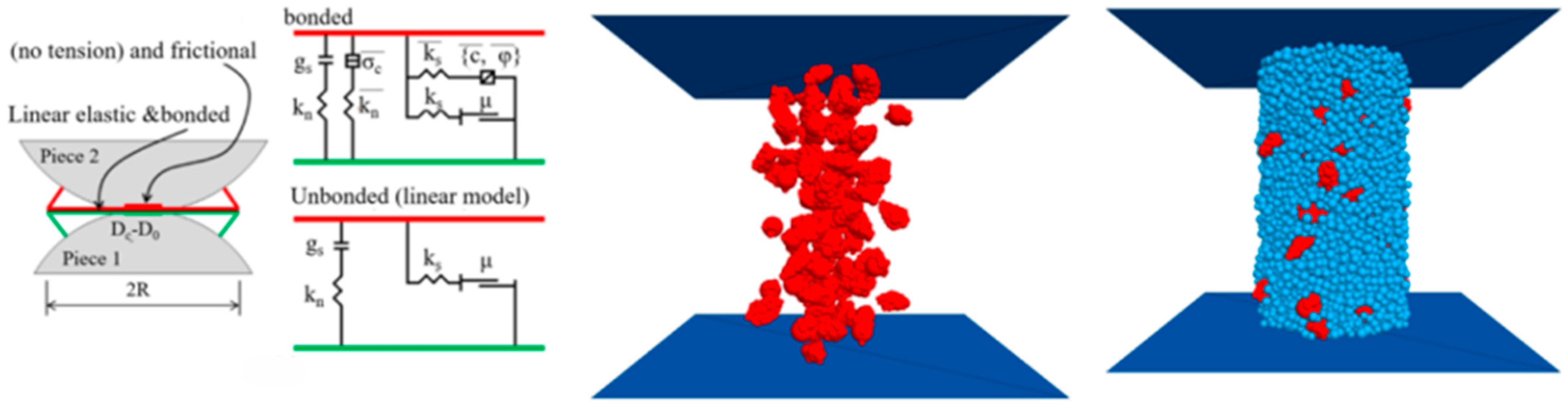
The spring element method (SEM) and discrete element method (DEM) are two core methods for numerical simulation in geotechnical engineering, and the choice depends on the characteristics of the problem. The SEM is based on continuum mechanics and efficiently simulates seismic wave propagation and the overall dynamic response of slopes. It is suitable for homogeneous soil slopes or continuous deformation scenarios. Based on the discrete medium theory, the DEM is good at simulating the discontinuous behavior of particles (such as fragmentation and rotation) and has prominent advantages in the analysis of jointed rock slopes and local instability. The application of both needs to be combined with the problem scale and computing resources: the SEM is used for the overall stability and dynamic parameter evaluation of slopes, while the DEM focuses on the local failure mechanism of slopes with complex structural surfaces (such as faults). In engineering, they are often used in combination. The SEM is used to evaluate the overall situation, while the DEM is used to refine key areas. The SEM has an advantage in efficiency in seismic wave field simulation, and the DEM has better accuracy in the destructive stage of strong earthquakes (such as liquefaction). Both have obvious limitations: the SEM is difficult to capture discontinuous deformation, and the computational complexity of the DEM increases exponentially with the number of particles, relying on parallel computing optimization. In the future, it is necessary to develop multi-scale coupling algorithms, improve the constitutive model of materials, and combine high-performance computing to break through the bottleneck of the particle number, providing a better solution for the dynamic stability of complex geological slopes. Our results show that the platform width, load type, and frequency of multi-stage slope have different degrees of influence on the dynamic magnification factor. In addition, the discrete element rule is more suitable for simulating rock slopes with many discontinuities. These discontinuities (such as joints) are often the key parts of landslides under cyclic micro-seismic action. By using the discrete element method, we can simulate the permanent displacement of the slope under the action of seismic waves and further study the law of the influence of the combination of slope height, seismic intensity, slope angle, and joint angle on the permanent displacement of the jointed rock slope. This method enables us to know more deeply the deformation and failure mechanism of the slope under the action of a micro-earthquake. In the numerical simulation, we also take into account the incidence of seismic waves, including both vertical and horizontal vibrations. By breaking down the vibration mode into these two basic forms, we can analyze the effect of ground motion on the slope more comprehensively. In addition, to simulate the real situation, we use a geometric model close to the actual slope scale and consider the influence of material parameters (such as elastic modulus, Poisson’s ratio, etc.) on the dynamic loading response results. Through the numerical simulation analysis, we not only obtained the stress distribution and displacement changes in the slope under the action of repeated micro-earthquakes but also further revealed the mechanical mechanism of landslide occurrence. These research results provide an important theoretical basis and practical guidance for slope seismic design and geological hazard protection.

When the rock and soil mass is in the stage of elastic deformation, its stress–strain relationship conforms to the elastic constitutive equation. For the plane stress problem, its elastic matrix is

$$[D]={\displaystyle \frac{E}{1-{\mu }^2}}\left[\begin{array}{lll}1\hfill & \mu \hfill & 0\hfill \\ \mu \hfill & 1\hfill & 0\hfill \\ 0\hfill & 0\hfill & (1-\mu )/2\hfill \end{array}\right]$$

(3)

In the above equation, [o] is the elastic matrix, and E is the elastic modulus of the material µ and Poisson’s ratio. If the material yields, its constitutive relation also changes accordingly. For the element of compressive (shear) failure, the total strain increment d {ε} is the sum of the elastic strain increment d {εe} and the plastic strain increment d {εp}, according to the increment theory:

$$d\left\{\epsilon \right\}=d\left\{{\epsilon }_e\right\}+d\left\{{\epsilon }_p\right\}$$

(4)

$$d\left\{{\epsilon }_e\right\}={[D]}^{-1}d\{\sigma \},d\left\{{\epsilon }_p\right\}=\lambda \left\{{\displaystyle \frac{\partial G}{\partial \sigma }}\right\}$$

(5)

The second equation is the flow law; if the associated flow law is used, then the plastic potential function can be used as the yield function f using the Drucke -Prager yield criterion, and

$$G=f=a{I}_1+\sqrt{J_2}-K$$

(6)

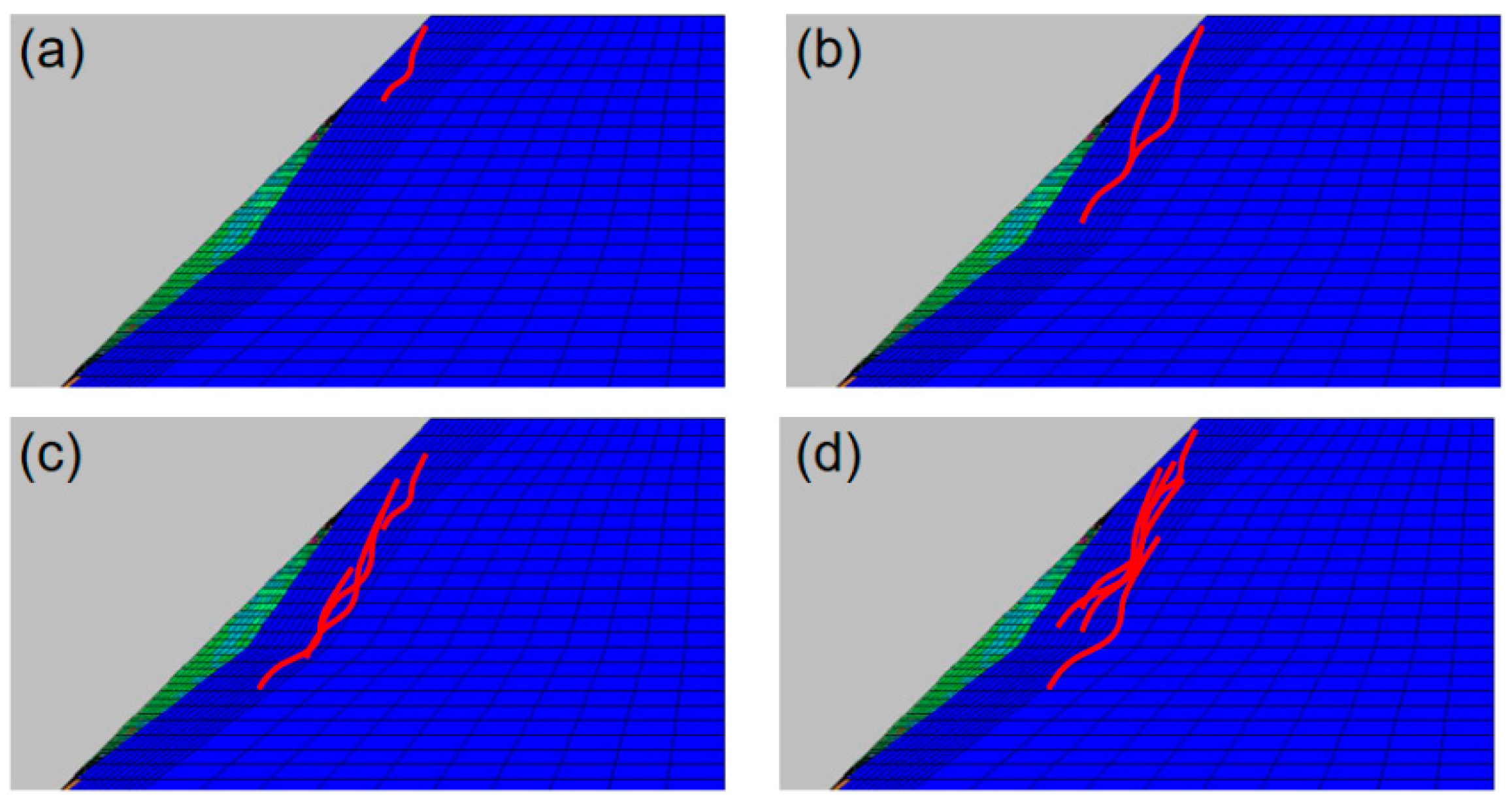
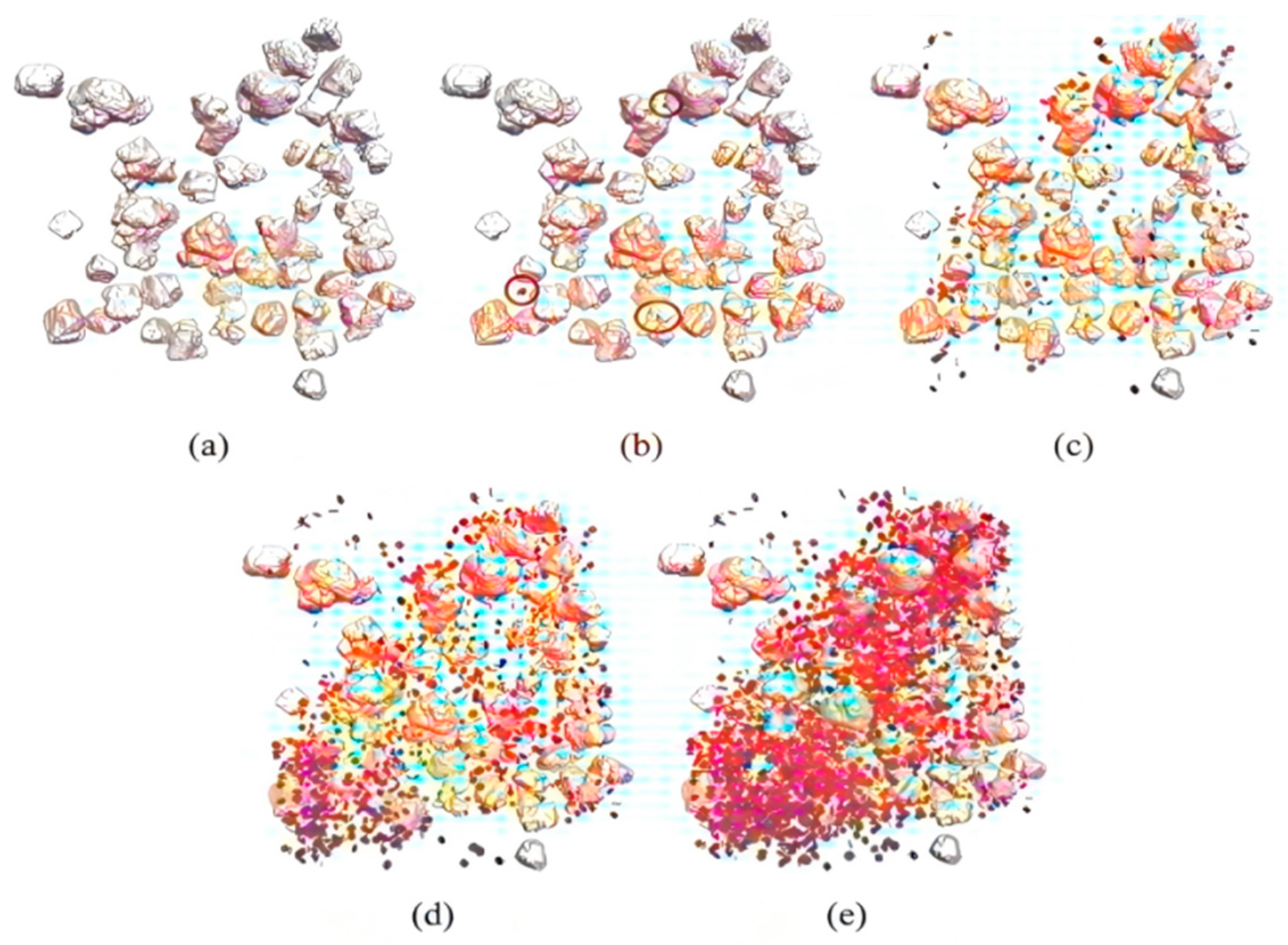
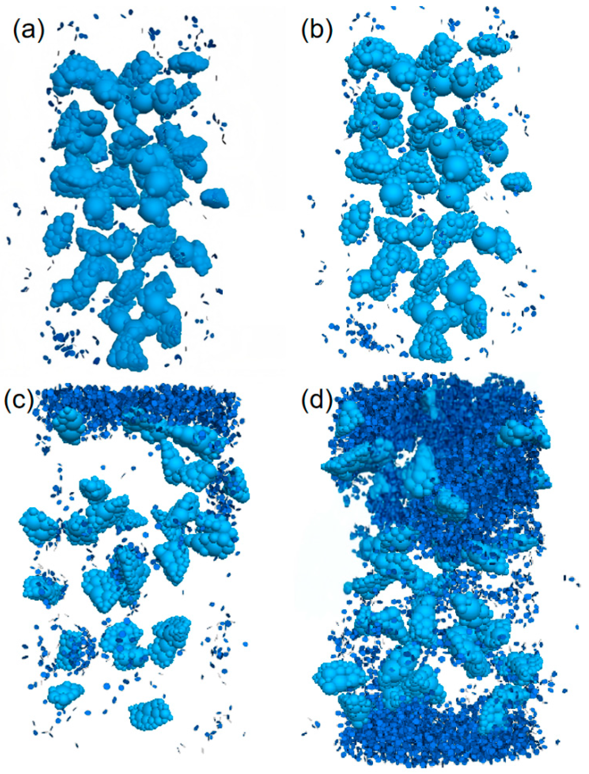
Under the action of a micro-earthquake, the cracks and joints inside the slope gradually expand and connect, which provides favorable conditions for the occurrence of landslides. The propagation of seismic waves leads to a change in the pore water pressure inside the rock and soil mass, especially at the moment when the seismic waves arrive; the sharp increase in pore water pressure will further reduce the shear strength of the rock and soil mass, thus accelerating the start of the landslide. In addition, the reflection and superposition effect of seismic waves inside the slope makes the stress concentration phenomenon more obvious in some areas, further aggravating the instability risk of the slope. First, according to the Piot theory, the saturated soil is first assumed to be a linear elastic medium, and the equilibrium equations in the consolidation and deformation process are derived by taking any differential element in the soil for analysis:

$${\displaystyle \frac{\partial {\sigma }_x^{\prime }}{\partial x}}+{\displaystyle \frac{\partial {\tau }_{yx}}{\partial y}}+{\displaystyle \frac{\partial {\tau }_{zx}}{\partial z}}+{\displaystyle \frac{\partial p}{\partial x}}-X=0$$

(7)

$${\displaystyle \frac{\partial {\tau }_{xy}}{\partial x}}+{\displaystyle \frac{\partial {\sigma }_y^{\prime }}{\partial y}}+{\displaystyle \frac{\partial {\tau }_{zy}}{\partial z}}+{\displaystyle \frac{\partial p}{\partial y}}-Y=0$$

(8)

$${\displaystyle \frac{\partial {\tau }_{XZ}}{\partial x}}+{\displaystyle \frac{\partial {\tau }_{yZ}}{\partial y}}+{\displaystyle \frac{\partial {\sigma }_Z^{\prime }}{\partial z}}+{\displaystyle \frac{\partial p}{\partial z}}-Z=0$$

(9)

where σ is the effective stress, p is the residual pore water pressure (including vibration pore water pressure), σ + p = σ is the total stress, and X, Y, and Z are the unit physical forces in the x-, y-, and z-directions. The geometric equation is then listed, where the compressive stress is positive, and the tensile stress is negative:

$${\epsilon }_x=-{\displaystyle \frac{\partial u}{\partial x}},\hspace{1em}{\gamma }_{yz}=-\left({\displaystyle \frac{\partial \omega }{\partial y}}+{\displaystyle \frac{\partial v}{\partial z}}\right)$$

(10)

$${\epsilon }_y=-{\displaystyle \frac{\partial v}{\partial y}},\hspace{1em}{\gamma }_{zx}=-\left({\displaystyle \frac{\partial u}{\partial z}}+{\displaystyle \frac{\partial \omega }{\partial x}}\right)$$

(11)

$${\epsilon }_z=-{\displaystyle \frac{\partial \omega }{\partial z}},\hspace{1em}{\gamma }_{xy}=-\left({\displaystyle \frac{\partial v}{\partial x}}+{\displaystyle \frac{\partial u}{\partial y}}\right)$$

(12)

where εx, εy, and εz are the positive strains of the soil skeleton in the x-, y-, and z-directions. Yx, yy, y, and z are the shear strains in the three directions. u, v, and W are the displacements of the soil skeleton in the x-, y-, and z-directions. Before the constitutive relation is proposed, the total strain {ε} is divided into two parts: one is the normal strain {ε-ε0}; another is the vibration strain {epsilon zero}, so {sigma} = {epsilon − epsilon zero} [D] = [D] {it} − {epsilon zero} [D].

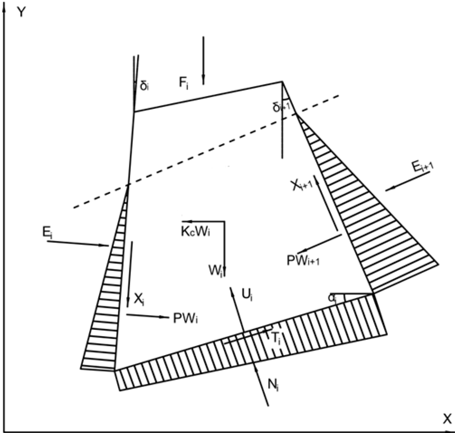
The Sarma method of slope limit equilibrium analysis is used to calculate the stability of a high and steep slope with faults, as shown in Figure 15. Taking any strip I in the slope body as an example, the working principle of the Sarma method is that, at any time, the transient stability coefficient of the sliding surface is F = 1, after the horizontal seismic inertia force term KW_c acting on the strip.

From the principle of static equilibrium, i.e., ΣX = 0 and ΣY = 0,

$$T_i\cos {\alpha }_i-N_i\sin {\alpha }_i-K_c{W}_i-F{X}_i-X_{i+1}\sin {\delta }_{i+1}+X_i\sin {\delta }_i-E_{i+1}\cos {\delta }_{i+1}+E_i\cos {\delta }_i=0$$

(13)

$$T_i\sin {\alpha }_i-N_i\cos {\alpha }_i-W_i+F{Y}_i-F_i+X_{i+1}\cos {\delta }_{i+1}-X_i\cos {\delta }_i-E_{i+1}\sin {\delta }_{i+1}+E_i\sin {\delta }_i=0$$

(14)

T_i and N_i are, respectively, the shear force and normal force acting on the bottom surface of strip I; W_i is the weight of strip I; X_i and X_i+1 are the shear forces acting on the I side and i+1 side, respectively; E_i and E_i+1 are the normal forces acting on the I side and i+1 side, respectively; F_i is the external load acting on the top of the slope; δ_i and δ_i+1 are the angles between the I side and the i+1 side and the vertical direction, respectively; α_i is the angle between the sliding plane of the I block and the horizontal direction.

From the Mohr–Coulomb criterion,

$$T_i=(N_i-U_i)\tan {\varphi }_{Bi}+c_{Bi}{b}_i\sec {\alpha }_i$$

(15)

Bi is the width acting on the bottom surface of block i; U_i is the water pressure acting on the bottom surface of block i; ${\phi }_{Bi}$ is the strength parameter of the bottom surface of block i. c_Bi.

$$X_i=(E_i-P{W}_i)\tan {\varphi }_{Si}+c_{Si}{d}_i$$

(16)

d_i and d_i+1 are the length of the i side and i + 1 side; PW_i and PW_i+1 are, respectively, the water pressure acting on the i and i+1 side, and ${\phi }_{Si}$ and $C_{Si}$ are the strength parameters of the i side. Through iterative calculation, different values can be calculated by using a different F value, and the F value at that time is the safety factor of the slope stability under the action of the natural earthquake inertia force. Previous models mostly simplified ground motion to a single frequency or static load, ignoring the propagation characteristics of the seismic spectrum (such as the energy distribution and phase difference in different frequency components) in rock and soil masses and their dynamic interaction with mesoscopic damage. For example, the synergistic effect between the local stress concentration effect caused by high-frequency waves and the cumulative effect of pore water pressure caused by low-frequency waves was not considered, nor was the influence of spectral characteristics (such as the main frequency and spectral width) on the crack propagation path quantified. 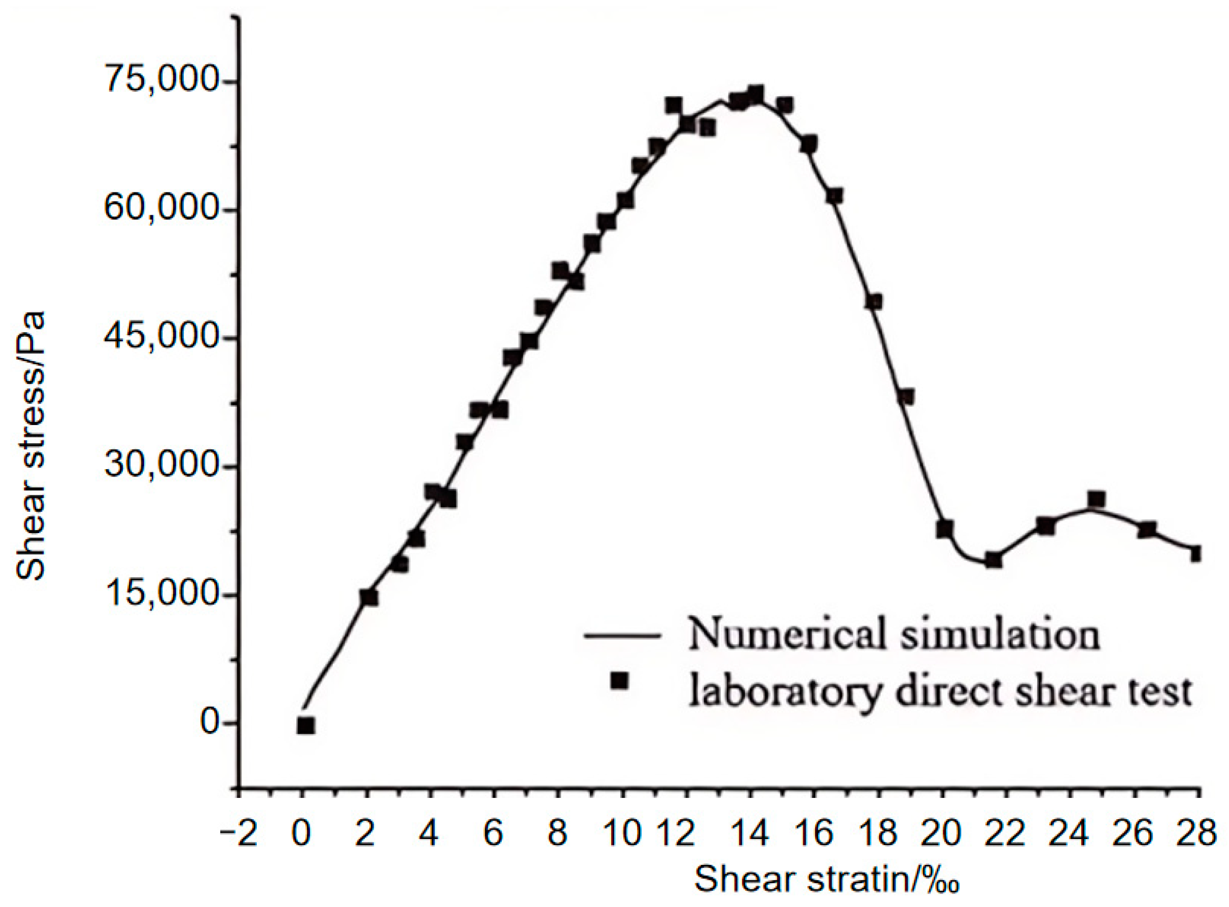The theories in Reference [24] are compared with the theoretical data and numerical simulation results of this paper, as shown in

Table 9. Comparison of different theories for slope stability.

Number of Cycles	Number of Cycles	The Theory of Literature 23	The Theory of This Article	Numerical Simulation
100	0.1	1.5	1.56	1.68
100	0.3	1.4	1.45	1.54
100	0.5	1.35	1.38	1.45
100	0.8	1.26	1.29	1.32
200	1.0	1.2	1.1	1.05
300	0.5	1.32	1.2	1.25
400	0.5	1.25	1.15	1.11
500	0.5	1.15	1.01	1.02

. By comparing Table 9, it can be seen that the theory in this paper is closer to the numerical simulation calculation results. The slope stability coefficient obtained by the theoretical calculation in this paper is closer to the numerical simulation, while the results of the traditional theory and numerical simulation calculation are relatively larger, indicating that the theoretical research results in this paper are more accurate.

4.2. Change the Rule of Slope Stability

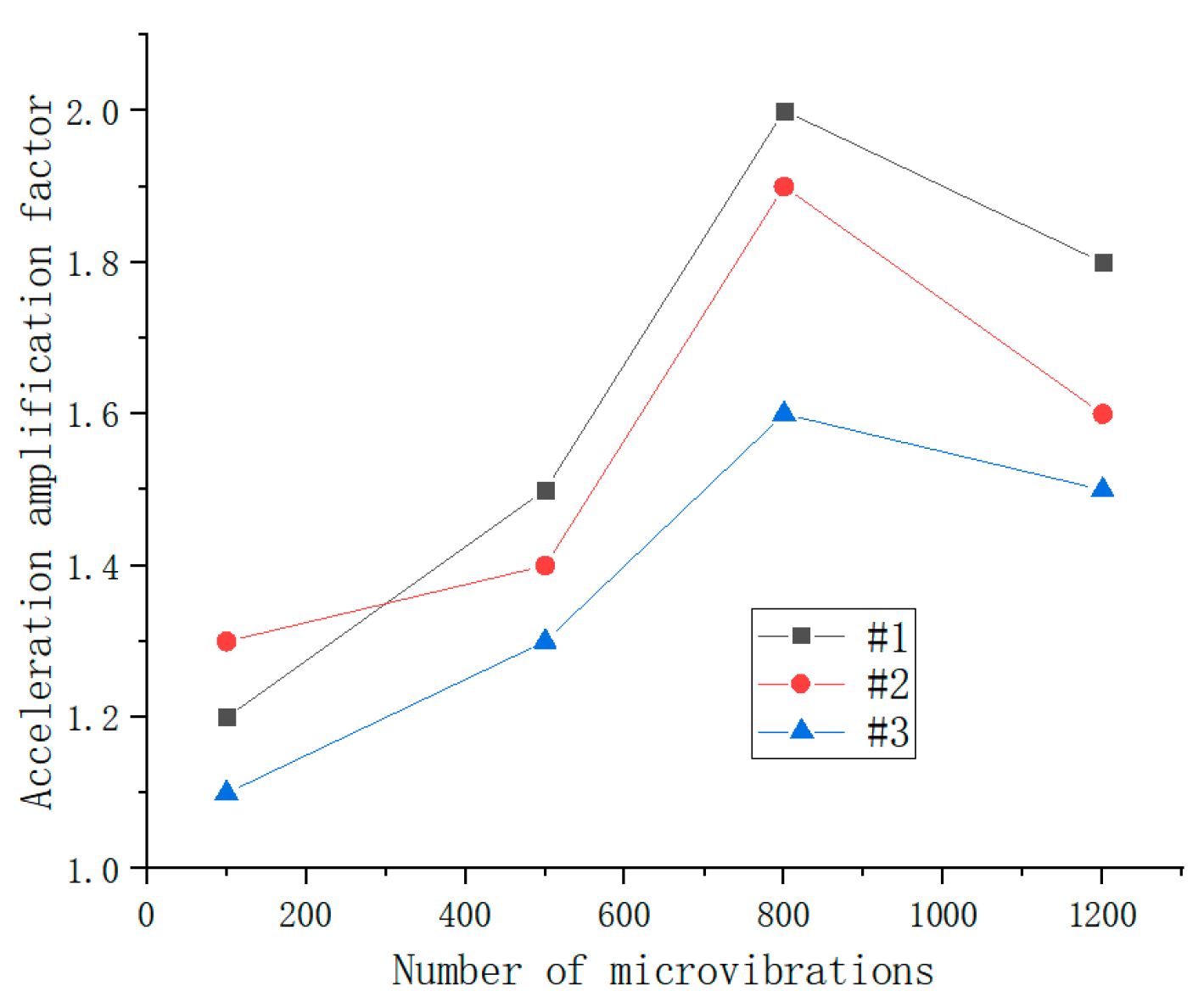
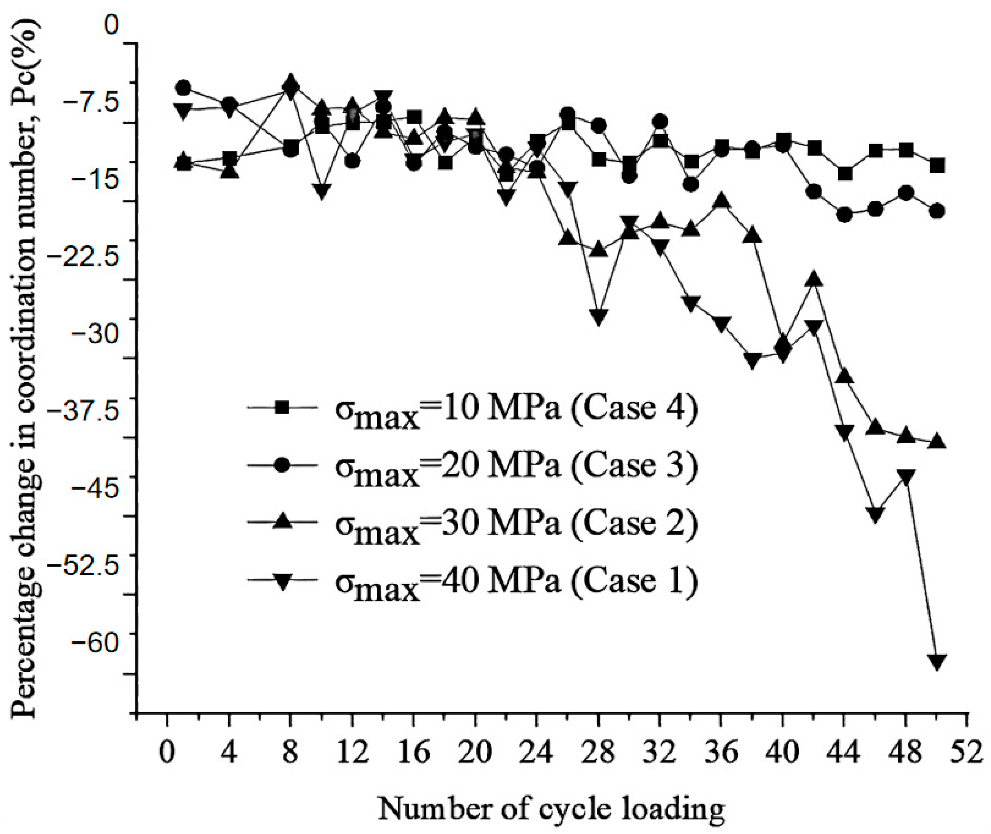
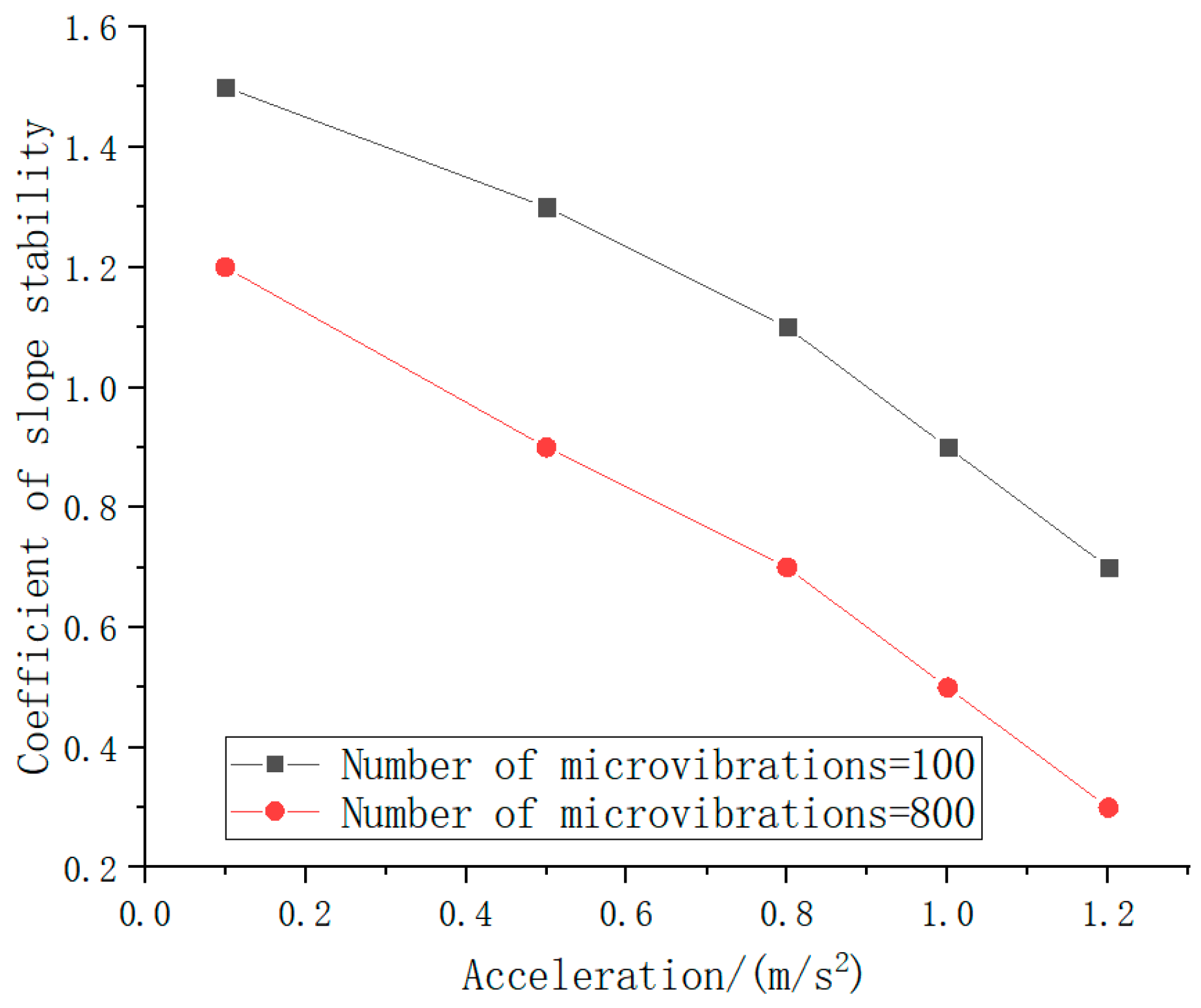
With the increase in seismic action times, the damage to the model slope continues to accumulate, the slope stability coefficient decreases with the vibration test, and the stability of the slope increases with the vibration times (100 times, 200 times, 300 times, 400 times, 500 times, 600 times, 700 times, and 800 times) and the vibration load strength (0.1 g, 0.5 g, 0.5 g, 0.5 g). 0.8 g, 1.0 g, and 1.2 g); the data change trend is shown in Figure 16.

The test data show that, with the increase in vibration times and load strength, the stability coefficient of the model slope presents a significant decreasing trend. And the higher the load strength, the greater the decline.

The decrease in the slope stability coefficient is mainly related to the influence of the vibration frequency and load strength on the accumulation of internal damage and the stress distribution of the slope. Under low load strength (e.g., 0.1 g), vibration mainly causes a slight expansion of the initial damage (e.g., plane, secondary joint, etc.) inside the slope and a small reduction in the stability coefficient (20%). With the increase in the load strength (e.g., 0.5 g~1.2 g), the expansion and penetration effect of vibration on the internal damage of the slope is significantly enhanced, resulting in a significant increase in the reduction in the stability coefficient (30.8~57.1%). In addition, the increase in vibration frequency further intensifies the cumulative effect of the internal damage of the slope, resulting in a continuous decline of the stability coefficient. At low load strength, the damage accumulation speed is slow, and the stability coefficient is relatively gentle. However, under high load strength, the damage accumulation speed is accelerated, and the decline of the stability coefficient is significantly increased. This changing trend reflects the synergistic influence of the vibration frequency and load intensity on the slope dynamic stability: the load intensity determines the degree of slope damage from a single vibration, while the vibration frequency determines the total effect of damage accumulation. The test results show that the slope stability coefficient has a non-linear decreasing trend with the increase in vibration times and load strength, which provides an important basis for the study of slope dynamic stability.

4.3. Deep Neural Network Model Training

A total of 200 sets of finite element calculation results were selected as the sample data set, which was divided into a 70% training set and a 30% test set by random allocation to ensure the uniformity of data distribution and avoid potential bias. To improve the efficiency and performance of the model training, the sample data were normalized, and all the data were scaled to the interval [0, 1] to monitor gradient changes and avoid overfitting or insufficient training during the model training process. After the training, the model’s performance was analyzed by a regression graph, and the following key indicators were obtained:

• The training regression coefficient is as high as 0.99607, indicating that the predicted value of the model has a high degree of fit with the actual value and can accurately capture the law of data change.
• The mean square error is only 0.00054, which is far lower than the preset error range, indicating that the model has a very high prediction accuracy.
• Analysis of training process: MSE is high in the initial stage, but with the increase in training times, MSE gradually decreases and tends to be stable by adjusting the weight and bias, while the value continues to rise, reflecting the gradual improvement of model prediction ability. To sum up, this study successfully constructed a neural network model with excellent performance through reasonable parameter settings and sufficient data training. The training results not only verify the reliability of the model but also reveal its strong potential in the evaluation of pipeline residual strength, which provides an important reference for the application of deep learning in the engineering field.

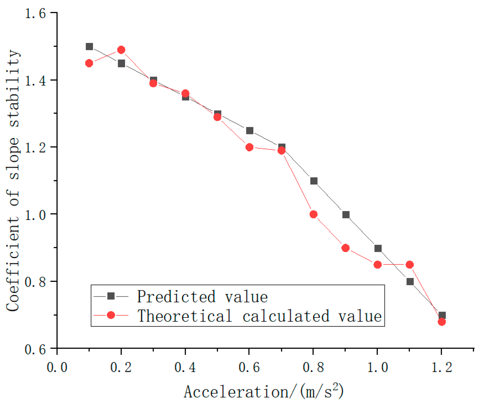
Although slope stability, as the only parameter to evaluate slope safety, has some limitations, based on its extensive engineering application background and a lot of research support, we believe that this index is reasonable and effective in the current study. To further verify the reliability of the deep learning-based neural network model in slope stability prediction, an independent test set was used in this study. This test set consists of the slope stability coefficient obtained from the test analysis, as shown in Figure 17. It covers a variety of corrosion patterns and severity. The independence and difference from the training set data are guaranteed, to comprehensively evaluate the generalization ability of the model. The verification results show that the neural network model not only performs well on specific data sets but also maintains highly accurate prediction ability in the face of unknown and diverse slope stability judgments, which reflects its strong generalization and robustness. Specifically, the prediction error of the model on the test set is significantly lower than the preset threshold, and the predicted results have a high degree of fitting to the actual values, which further confirms its reliability.

Based on the above verification results, this study indicates that the BP neural network model has high reliability and practicability in evaluating slope stability. The predicted results can provide an important reference for engineering practice and help to provide more accurate slope maintenance, repair, or replacement strategies, to ensure the safety and stability of the slope. These research results not only deepen the application of deep learning in slope stability assessment but also provide new technical support for related engineering fields.

5. Conclusions

Quantitative characterization of the sustainable performance of tailings concrete: A two-parameter damage model of strength loss rate and crack number was established through cyclic load tests to confirm the feasibility of tailings replacing natural aggregates in a vibrating environment. The strength attenuation rate of tailings is 15–20% lower than that of ordinary concrete, significantly reducing the consumption of natural resources (saving 120 kg of sand and gravel per cubic meter of concrete).

Load–damage coupling mechanism: The cycle number dominates the long-term deterioration through the accumulation of defects in the interface transition zone (with ITZ cracks accounting for 72%) and energy dissipation (converting 20% of mechanical energy into crack propagation energy in a single cycle), and the load amplitude controls the instantaneous damage evolution through the change in the stress state (triaxial stress coupling increases the crack propagation rate by 2.5 times). A parameter basis for the engineering design of vibration equipment foundations, traffic load pavements, etc. is provided.

Eco-friendly design threshold: We recommend determining the 0.5 g acceleration amplitude as the ecological critical threshold. When it exceeds this threshold, the internal crack density of the concrete exceeds 1.5 cracks /mm², resulting in a 30% increase in the risk of damage to the seepage channels of the soil around the service structure. It is recommended to optimize the slope protection structure in combination with the terrain amplification effect (the top acceleration amplification coefficient reaches 2.0). We recommend reducing the ecological chain damage caused by earthquakes.

Sustainable engineering application strategy: A dual-track regulation method of “priority control of load amplitude + intelligent monitoring of cycle times” is proposed. In high-cycle conditions (such as mechanical vibration foundations), keeping the load amplitude below 0.3 g can extend the service life by 40%. In high-amplitude environments (such as earthquake-prone areas), preventive maintenance is achieved through real-time monitoring of crack density (critical value 1.5 cracks/mm²), reducing carbon emissions throughout the entire life cycle by more than 25%.