Short-Term Power-Generation Prediction of High Humidity Island Photovoltaic Power Station Based on a Deep Hybrid Model

Abstract

Precise prediction of the power generation of photovoltaic (PV) stations on the island contributes to efficiently utilizing and developing abundant solar energy resources along the coast. In this work, a hybrid short-term prediction model (ICMIC-POA-CNN-BIGRU) was proposed to study the output of a fishing–solar complementary PV station with high humidity on the island. ICMIC chaotic mapping was used to optimize the initial position of the pelican optimization algorithm (POA) population, enhancing the global search ability. Then, ICMIC-POA performed hyperparameter debugging and L2-regularization coefficient optimization on CNN-BIGRU (convolutional neural network and bidirectional gated recurrent unit). The L2-regularization technique optimized the loss curve and over-fitting problem in the CNN-BIGRU training process. To compare the prediction effect with the other five models, three typical days (sunny, cloudy, and rainy) were selected to establish the model, and six evaluation indexes were used to evaluate the prediction performance. The results show that the model proposed in this work shows stronger robustness and generalization ability. K-fold cross-validation verified the prediction effects of three models established by different datasets for three consecutive days and five consecutive days. Compared with the CNN-BIGRU model, the RMSE values of the newly proposed model were reduced by 64.08%, 46.14%, 57.59%, 60.61%, and 34.04%, respectively, in sunny, cloudy, rainy, continuous prediction 3 days, and 5 days. The average value of the determination coefficient $R^{2 }$of the 20 experiments was 0.98372 on sunny days, 0.97589 on cloudy days, and 0.98735 on rainy days.

1. Introduction

In recent years, the global focus on developing clean energy sources has led to the increasing prominence of solar energy as a viable alternative for meeting energy demands [1,2]. Photovoltaic (PV) stations are categorized into land-based and water-based stations, depending on their geographical location. Land-based PV stations have a well-established power-generation technology, while water-based PV stations have emerged as a relatively new type of facility in recent years. The PV array is primarily installed on lakes, reservoirs, or oceans, thereby minimizing land usage [3,4]. This approach offers the advantage of maximizing the synergistic benefits between power generation and aquaculture, commonly referred to as the “upper power generation, lower aquaculture” concept. Placing solar panels on the water’s surface provides shading for fish, improves the local water temperature, and enhances the economic returns of aquaculture. Additionally, the higher relative humidity around the solar panels contributes to reduced module temperature and, consequently, enhances the photoelectric conversion efficiency of the solar panels to some extent. The power generation of water-based PV stations surpasses that of land-based PV stations when considering the same area [5]. Accurately and swiftly predicting the power generation of PV stations [6,7,8,9] enables enterprises to develop timely power-scheduling plans, addressing the issue of temporal mismatch between supply and user demand. This facilitates timely adjustment of electricity prices and maximizes the promotion of user demand for power consumption, enhancing demand-side flexibility and mitigating excess power generation. These objectives align well with China’s “dual-carbon” goals. Consequently, the establishment of a high-precision prediction model with robustness and a strong generalization ability holds significant importance.

With the rapid advancement of artificial intelligence algorithms, an increasing number of algorithms are being employed for solar power prediction. Direct prediction utilizing data-driven algorithm models has proven to be more reliable and accurate compared to indirect prediction methods [10]. Traditional machine-learning techniques, such as principal-component analysis (PCA) [11,12], variable modulus decomposition (VMD) [13], and random forest (RF) [14], are utilized for data-feature extraction and prediction. Additionally, support-vector machine (SVM) [15], artificial neural network (ANN) [16], Elman neural network [17], radial basis function neural network (RBF) [18], Bayesian methods [19], among others, are employed for power-generation prediction. For instance, in references [20,21], SVM was utilized to enhance the accuracy of PV power-generation prediction. Reference [22] used VMD to extract feature variables and input them into the ANN model to predict the output power of the PV system. In Reference [23], the K-means algorithm was utilized to cluster different weathers, and Elman served as the prediction model to improve the prediction accuracy and robustness. The literature [24] employed PCA to extract data-feature information and reduce dimensionality, which was then fed into a generalized regression neural network (GRNN) model for prediction.

The aforementioned methods often exhibit limitations in data mining, as they tend to focus on shallow feature extraction without delving into deeper internal feature information. Consequently, their data-driven capabilities are relatively general [25]. When faced with the challenge of predicting power generation in the presence of high volatility, shallow learning models may produce significant errors. To address these issues effectively, deep learning models offer promising solutions.

The deep learning model exhibits a more intricate network structure compared to the shallow learning model, enabling it to effectively express complex functions and possess deep learning capabilities. Notably, the convolutional neural network (CNN) and time convolutional network (TCN) [26] excel in data-feature extraction. These models can adeptly capture temporal dependencies in sequential data, showcasing robust data depth mining and feature information-extraction capabilities. Such performance is not attainable with shallow learning models. Deep learning models, including stacked autoencoder (SAE) [27,28], deep belief network (DBN) [29,30], recurrent neural network (RNN) [31], and enhanced variants of long short-term memory (LSTM) [32,33] and gated recurrent unit (GRU) [34], offer enhanced accuracy and stability in prediction. In References [1,35], CNN was employed for data filtering and denoising, while the pooling layer reduced data dimensionality and memory requirements and improved processing speed. By establishing deep connections between feature information and leveraging its memory unit, LSTM achieved high-precision prediction outputs. References [36,37] proposed a hybrid CNN-GRU model to minimize power-prediction errors. In [38], the accuracy of the LSTM-RNN prediction model was enhanced through a time-dependent correction method. Reference [39] introduced the LSTM-TCN hybrid model, which demonstrated superior prediction performance compared to single models across diverse weather conditions and multiple time-prediction periods.

It is worth noting that the adjustment of hyperparameters is crucial for harnessing the strong learning ability of deep learning models. Manual adjustment or traditional methods for hyperparameter optimization can be time-consuming and costly, making them impractical for enterprises. To efficiently address this optimization problem, heuristic optimization algorithms offer a viable solution. These algorithms employ automatic iteration to rapidly converge to the global optimal value by considering constraints, objective functions, and decision variables. They are capable of effectively solving various hyperparameter-optimization combination problems [31]. Examples of such algorithms include genetic algorithm (GA) [40,41,42], particle-swarm optimization (PSO) [43,44], firefly algorithm (FA) [45], ant-colony algorithm (ACO) [21], bat algorithm (BA) [46,47], and others.

Limited research has been conducted on the prediction of fishing–solar complementary PV stations. In this study, we propose a hybrid prediction model, ICMIC-POA-CNN-BIGRU, which leverages historical PV power-generation data and numerical weather prediction (NWP) meteorological data as the original dataset to drive the algorithm. The CNN component of our model effectively mines the relevant information between PV power generation and power-generation variables, extracting deep features from the data. These features are then inputted into the bidirectional gated recurrent unit (BIGRU) component for prediction. BIGRU, consisting of two GRUs, processes sequence data bidirectionally, enabling the model to capture deep feature information before and after specific moments and enhance its generalization ability. To efficiently optimize the hyperparameter combination of CNN-BIGRU, we utilize the latest heuristic optimization algorithm, the pelican optimization algorithm (POA). Additionally, the ICMIC chaotic mapping technique optimizes the initial population position of POA, preventing the model from getting stuck in local optima and improving global convergence speed. It is worth noting that the shortcoming of the hybrid model relative to the single model is the increase in computational cost. The main contributions of this study are summarized as follows:

• Combining CNN’s powerful data-feature extraction ability with BIGRU’s two-way use of time series prediction, the latest heuristic algorithm (POA) is proposed for the first time to optimize CNN-BIGRU hyperparameters;
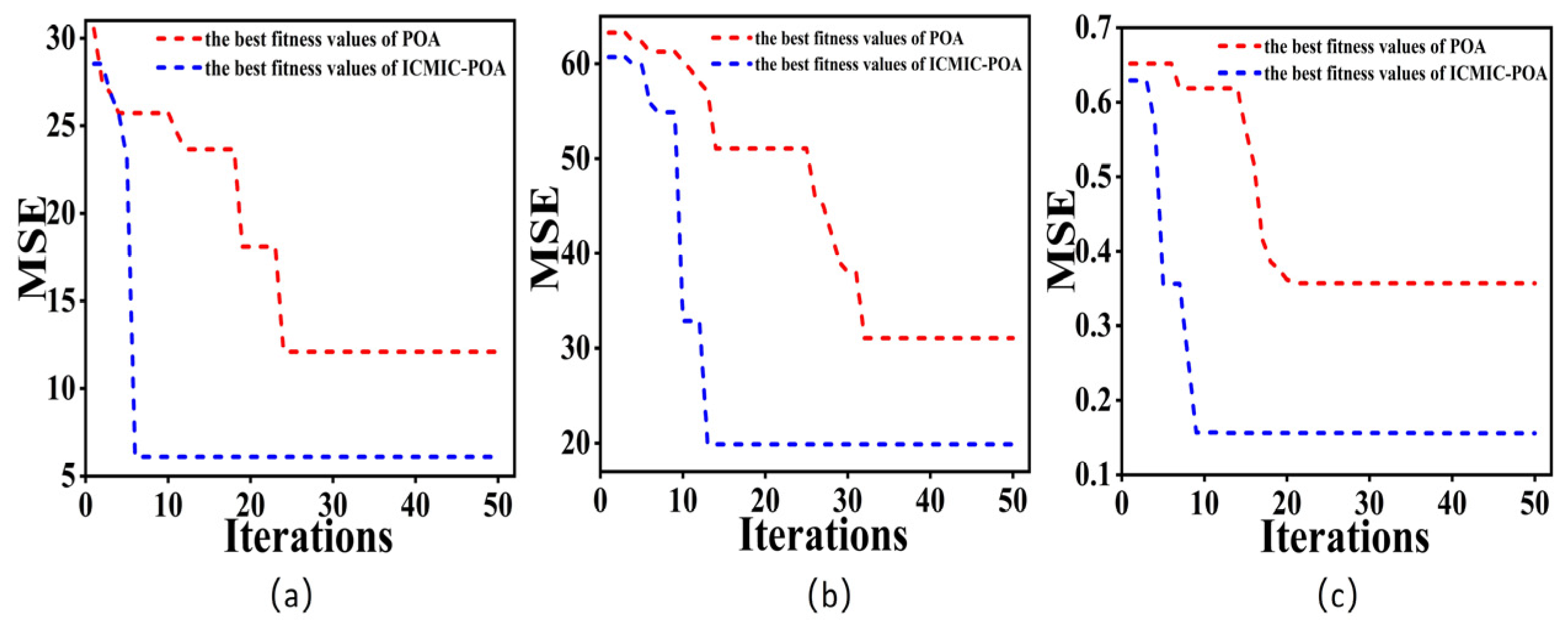
• To enhance the convergence speed and global optimization ability of the algorithm, the ICMIC chaotic mapping technique is employed to optimize the initialization position of the POA population;
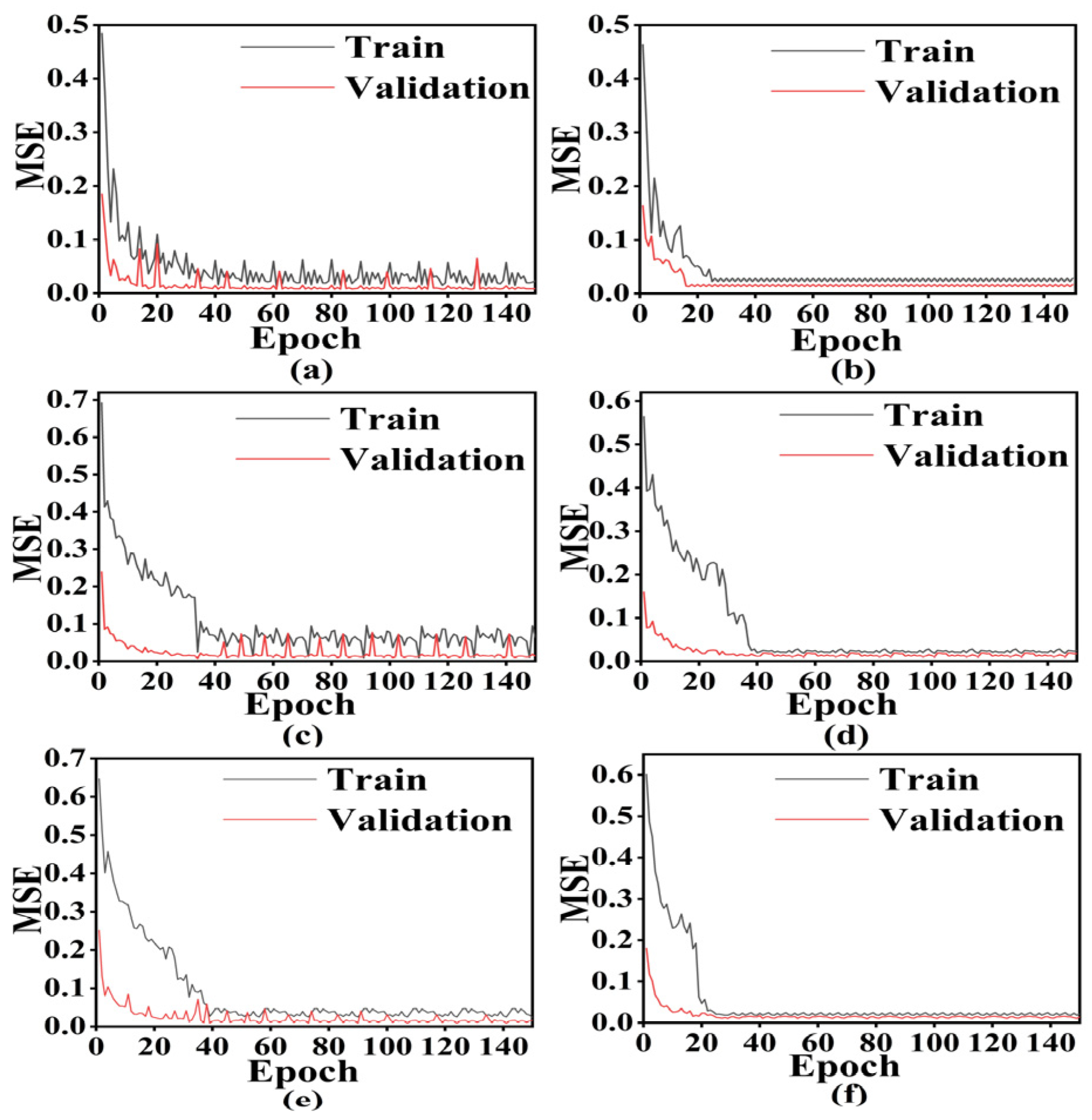
• To address potential overfitting issues during training, the L2-regularization technique is employed, which facilitates rapid convergence of the loss curve for CNN-BIGRU. Furthermore, the optimal L2-regularization coefficient is automatically iteratively optimized using the POA algorithm;
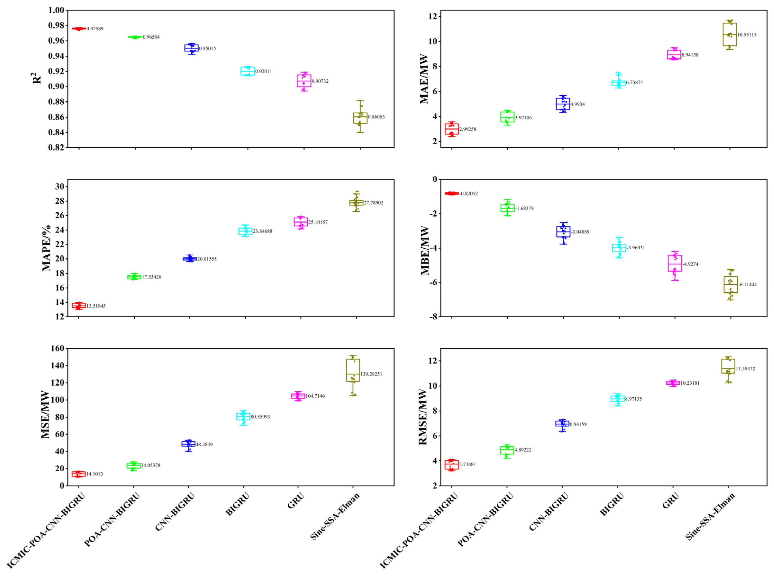
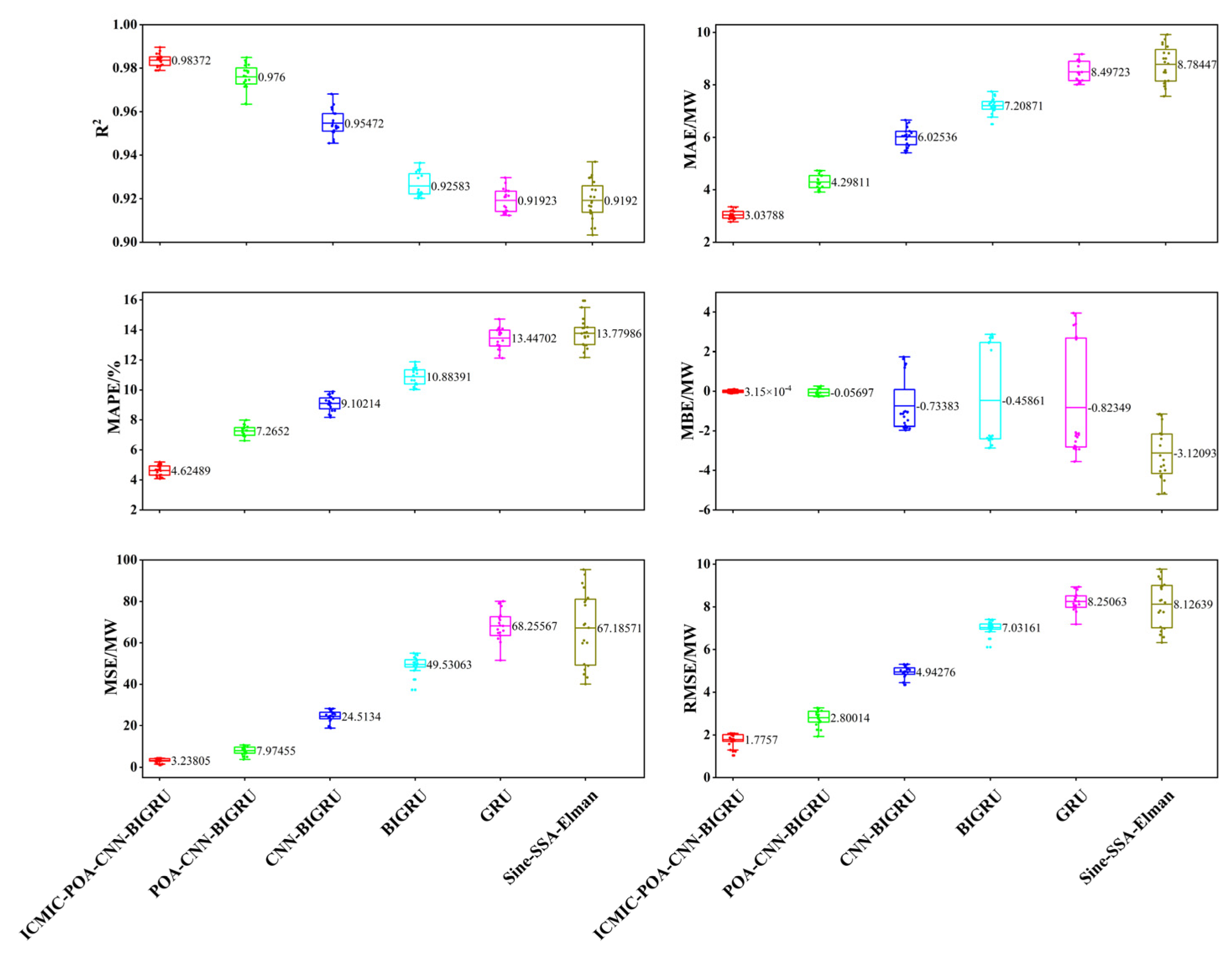
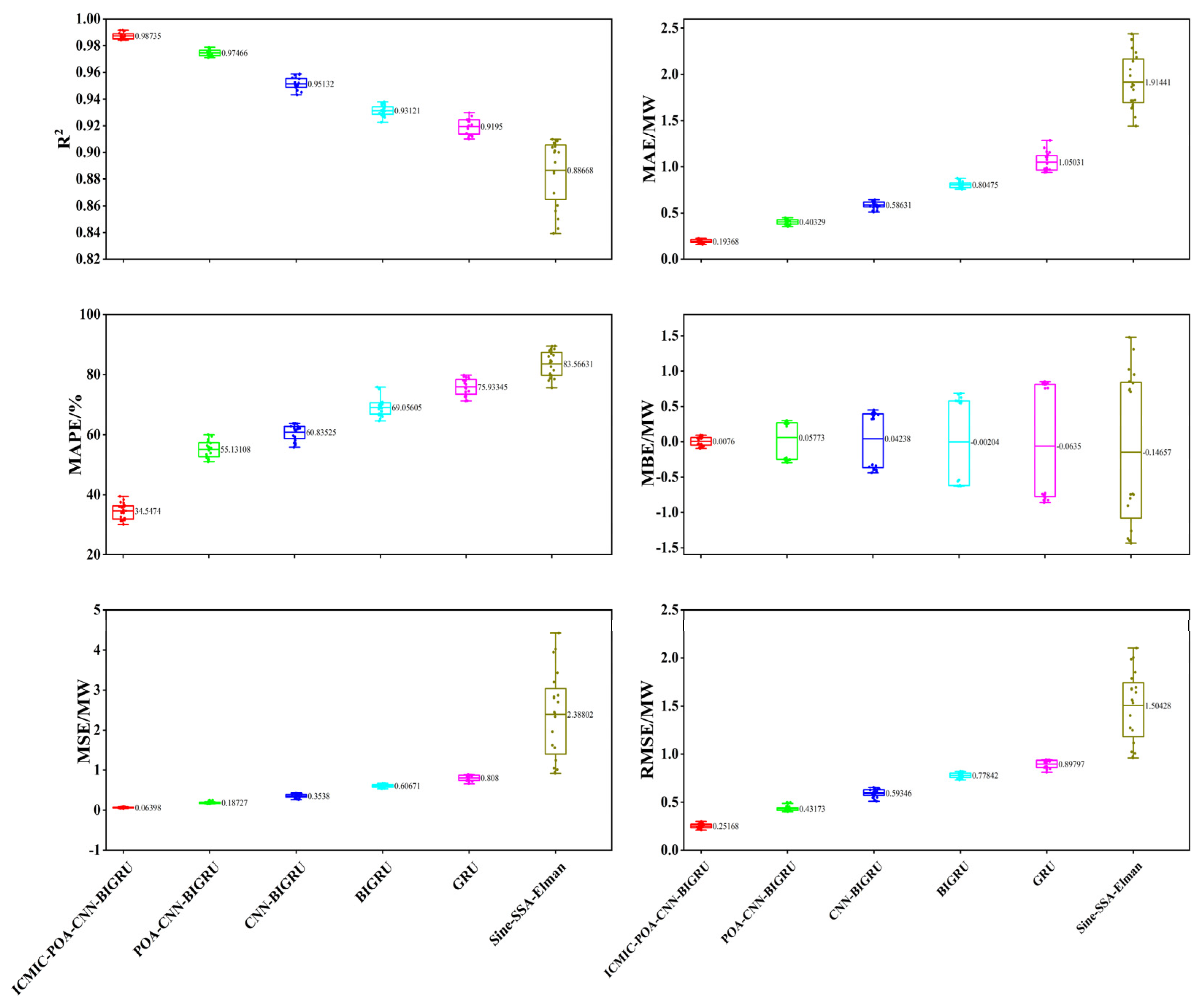
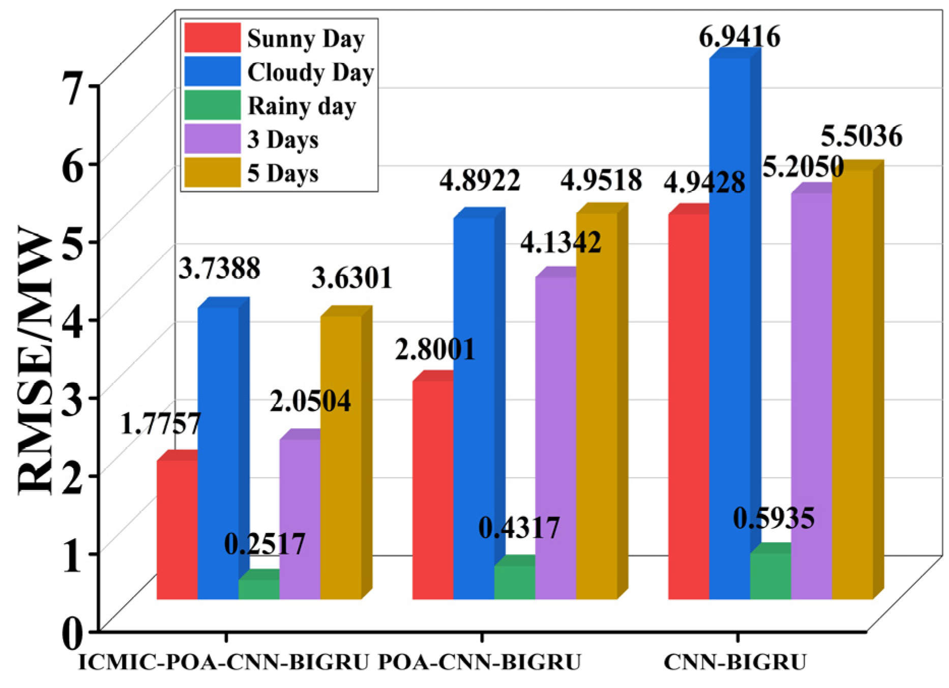
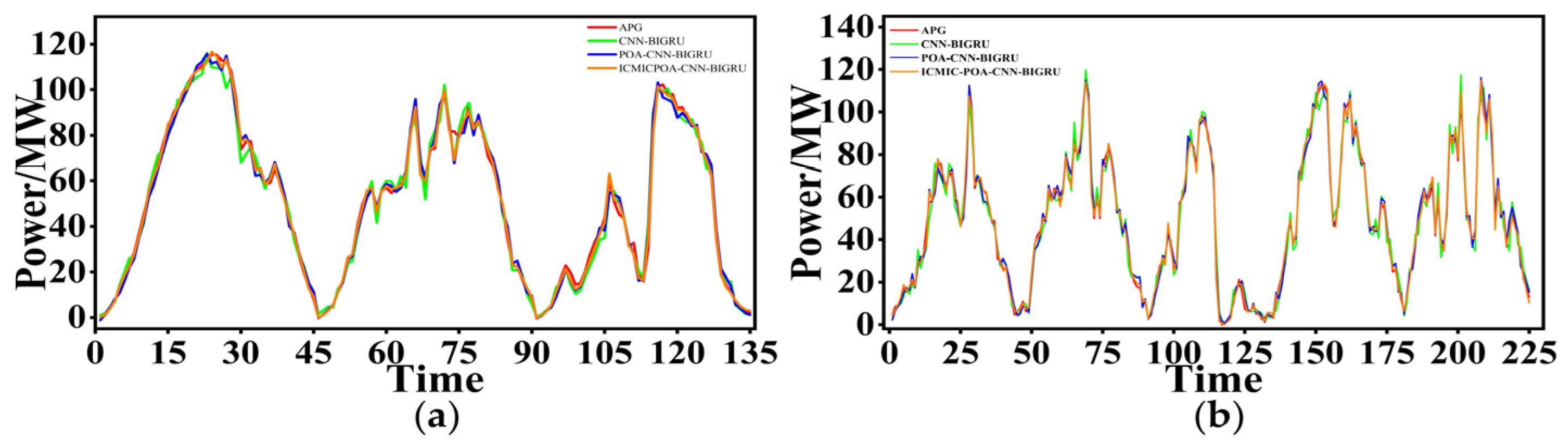
• The prediction performance of the six models under diverse weather conditions is evaluated using six evaluation indicators. K-fold cross-validation is conducted to compare the prediction effects of the three hybrid models on different datasets spanning three consecutive days and five consecutive days. The results demonstrate that the hybrid model proposed in this study exhibits the most superior prediction performance.

Section 2 introduces the source of the data and provides a detailed explanation of the data preprocessing methods and the working principles of the hybrid prediction model; Section 3 discusses the prediction results of the different test sets; Section 4 draws a conclusion.

2. Materials and Methods

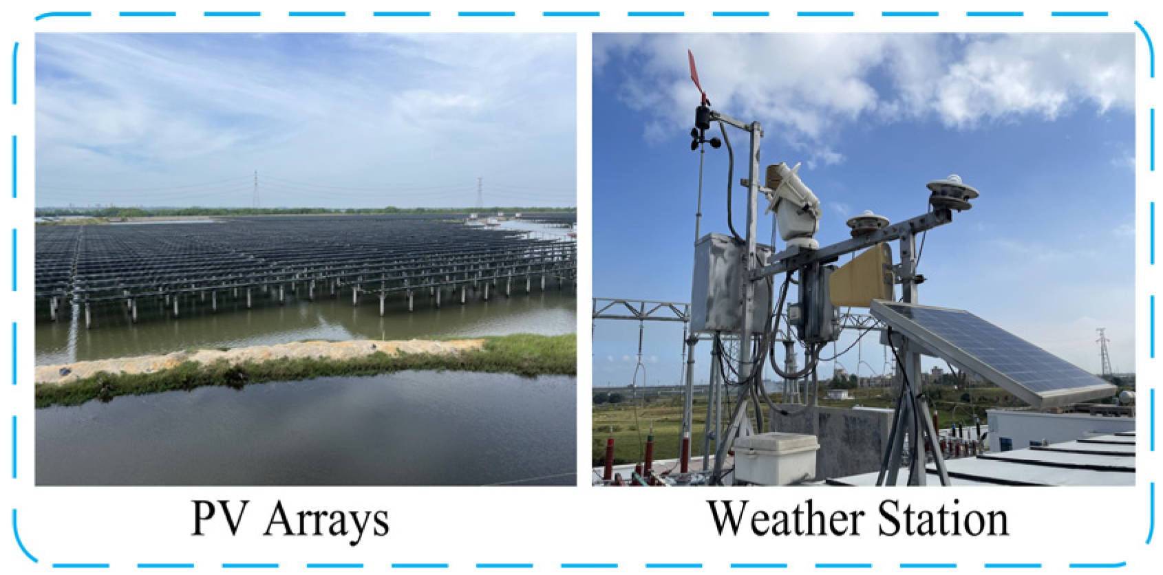
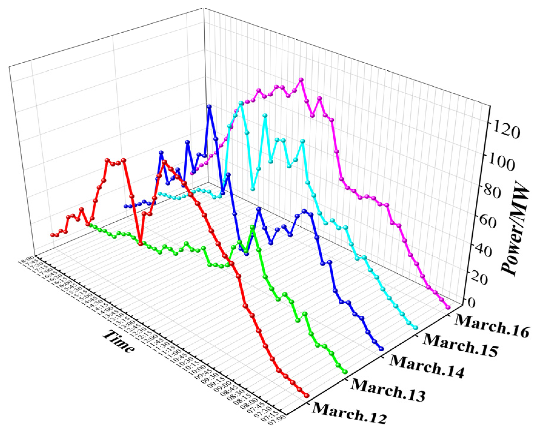
2.1. Data Sources

For this study, we conducted prediction research using a fishing–solar complementary PV power station with an installed capacity of 100 MWp, located in the East China Sea Island (110.38° E, 21.03° N) of Guangdong Province, China. This PV station serves as our experimental platform. Situated in close proximity to the sea, the station benefits from abundant solar irradiation resources, high temperatures, minimal rainfall, and extended daily sunshine hours, making it an ideal location for PV power generation. Notably, the solar panels are tilted and positioned above the water surface, reducing dust deposition compared to terrestrial environments. However, this arrangement leads to increased water evaporation and remarkably high relative humidity. Figure 1 displays the PV arrays and the weather station of the PV station, which enable data monitoring and collection.

While numerous prediction studies have been conducted on various types of PV stations characterized by low relative humidity, we deliberately concentrate on a distinct aspect by focusing on the time intervals exhibiting high relative humidity. Specifically, we observe that during the months of March to May, there is a greater probability and frequency of rainfall, thereby accentuating the elevated relative humidity levels specific to the fishing–solar complementary PV power station. We obtained a two-month dataset (5 March 2023 to 4 May 2023) from the collection-monitoring system and the weather station database. The data was collected at 15 min intervals within the time range of 7:00–18:00. The original dataset includes 19,215 sets of data, including normal direct irradiance (NDI, $\mathrm{W}/{\mathrm{m}}^2$), global horizontal irradiance (GHI, $\mathrm{W}/{\mathrm{m}}^2$), scattered irradiance (SI, $\mathrm{W}/{\mathrm{m}}^2$), ambient temperature (AT, °C), relative humidity (RH, %), module temperature (MT, °C), and actual power generation (APG, MW). Figure 2 illustrates the actual power generation observed from 12 March 2023 to 16 March 2023.

2.2. Data Preprocessing

High-quality data is the basis of data analysis and driving. Conversely, low-quality data can significantly impact the learning ability of prediction models and result in suboptimal prediction outcomes. Within the PV-station system, equipment failures are inevitable and can lead to deviations in the recorded real data, consequently diminishing the quality of the dataset. To address this issue, employing data preprocessing methods can effectively enhance the data quality.

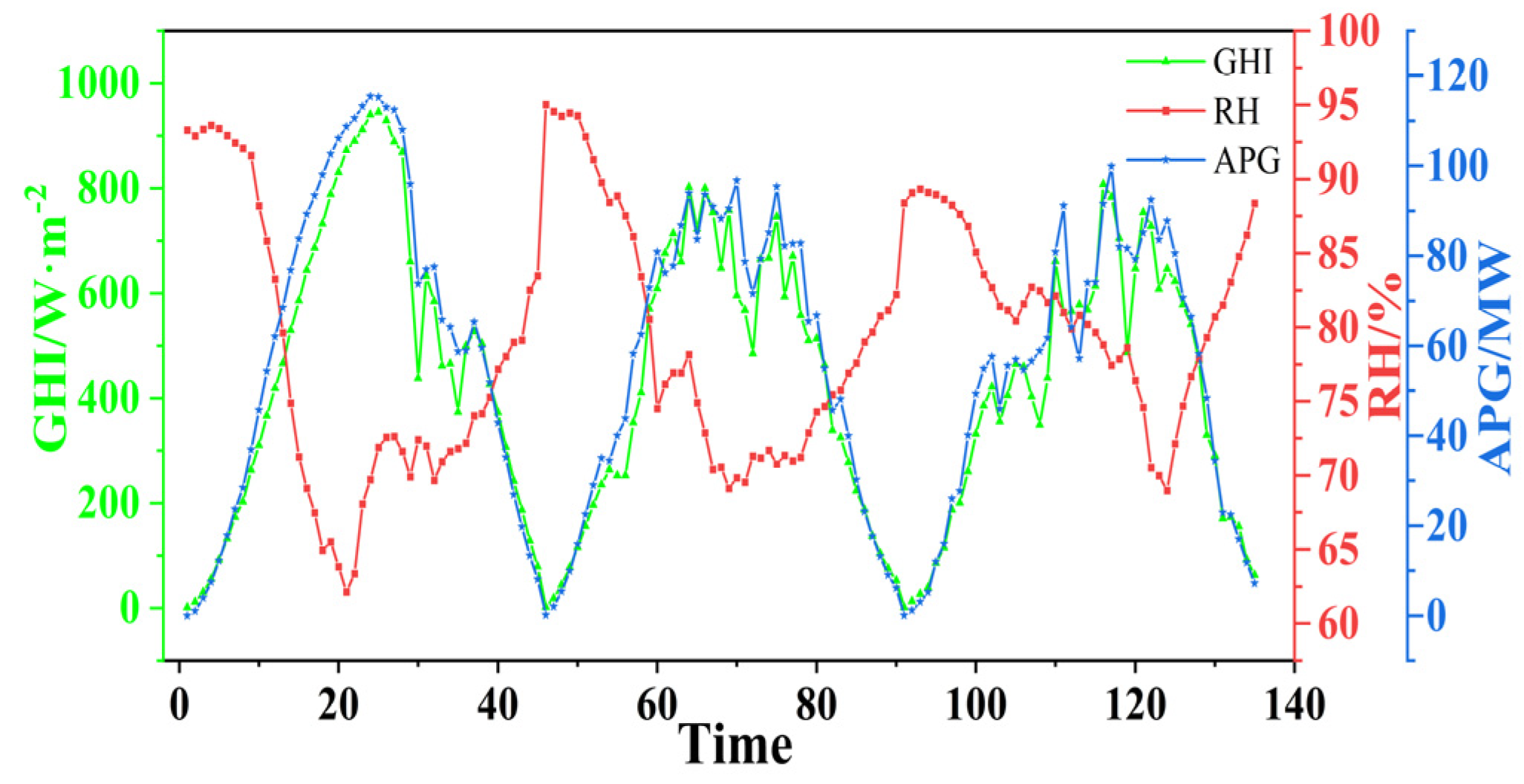
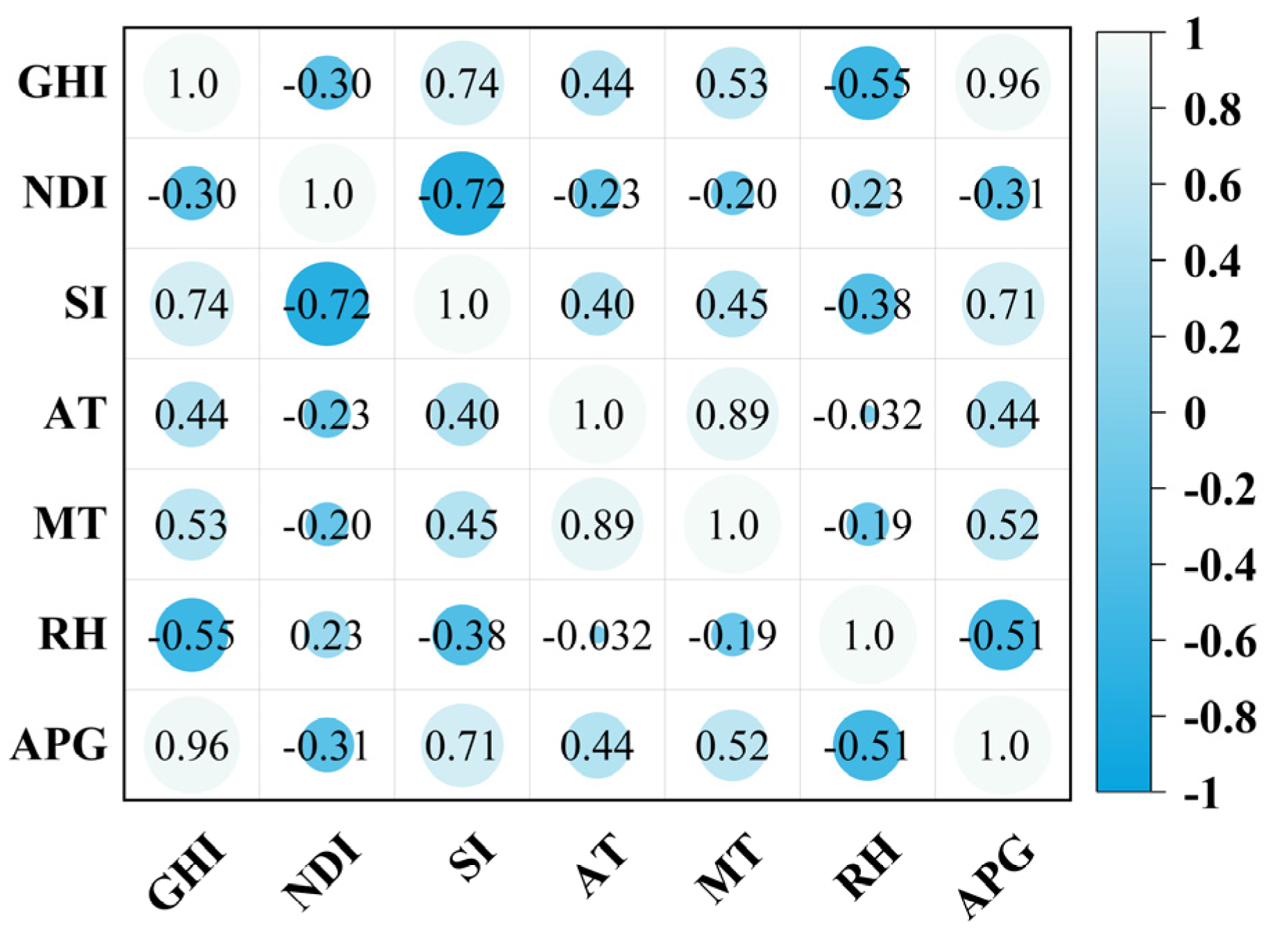
2.2.1. Correlation Analysis

The data contained within the PV power-station database exhibits nonlinear relationships across different types. To assess the degree of nonlinear correlation between variables, the Spearman correlation coefficient (SCC) is employed. Unlike the Pearson correlation coefficient (PCC), SCC is a non-parametric rank correlation measure that offers enhanced robustness and better handling of outliers. Moreover, SCC remains unaffected by dimensionality and can effectively measure the correlation between variables even in the presence of missing data. The calculation of the Spearman correlation coefficient ($\rho$) is as follows:

$$\rho =1-6{\sum }_{i=1}^n{d}_i^2/n(n^2-1)$$

(1)

where $d_i$ is the rank order difference, $n$ is the number of samples, $\rho ϵ\left[-\mathrm{1,1}\right]$, and $\left|\rho \right|$, the closer to 1, indicates the stronger correlation between the two variables.

Figure 3 illustrates the SCC analysis conducted on the variables within the original dataset. The variable exhibiting the strongest correlation with APG is GHI, with a coefficient of 0.96, indicating a highly significant correlation. SI (0.71), MT (0.52), RH (−0.51), and AT (0.44) also display notable correlations with APG. It is worth noting that solar irradiance directly impacts the power-generation efficiency of PV panels. Furthermore, particular attention must be given to the influence of high RH environments on PV-panel power generation. High RH levels can also affect the module and ambient temperatures of PV panels. To support these findings, Figure 4 presents a three-day record of GHI, RH, and APG, further confirming the results of the correlation analysis.

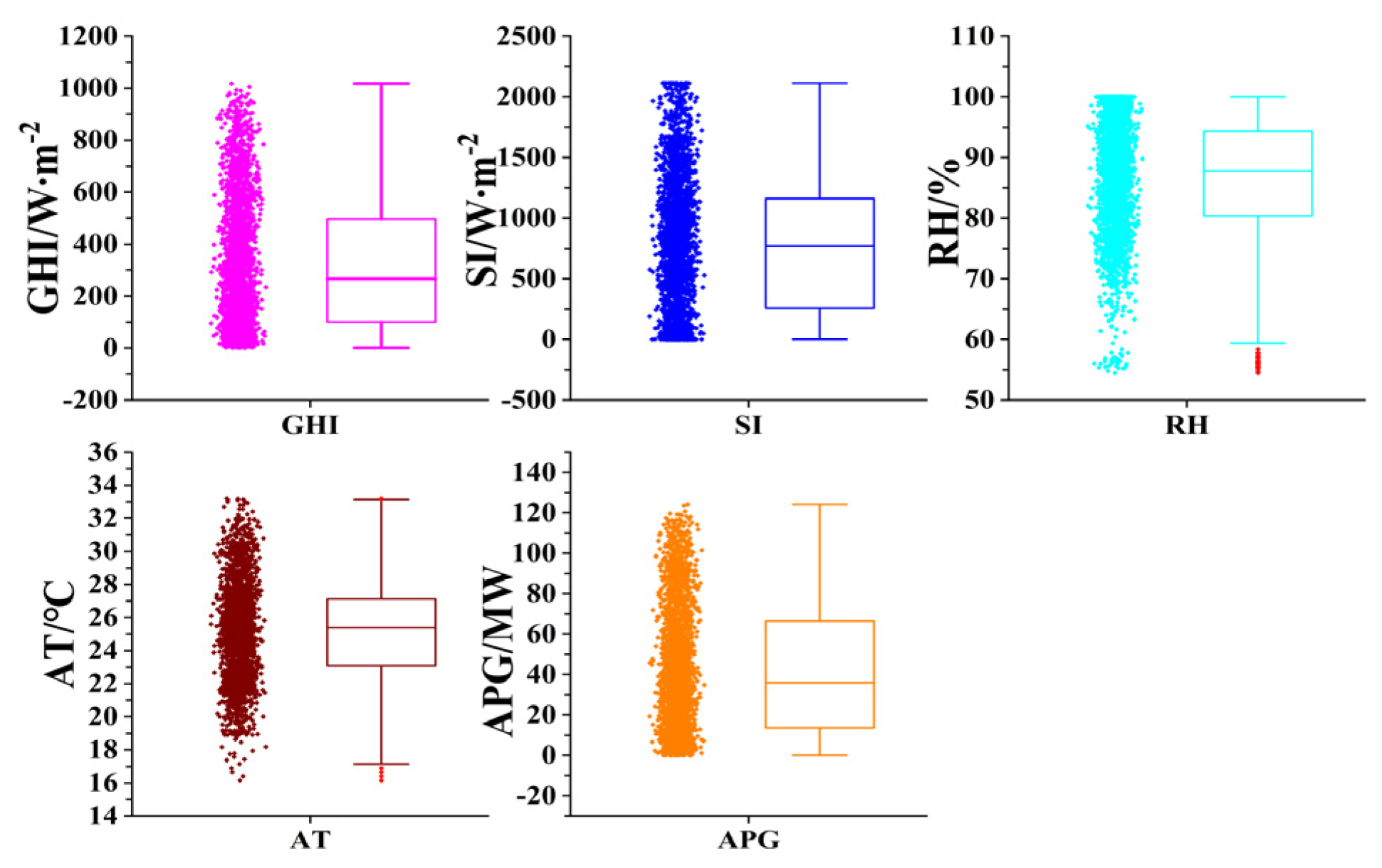
2.2.2. Outlier Processing

The data outliers in this study encompass both missing values and non-conforming values. To address this issue, two variables were removed: NDI (−0.31), which exhibited a weak correlation with APG, and MT (0.52), which did not pertain to meteorological data. Subsequently, four external meteorological variables (GHI, SI, RH, and AT) that were significantly correlated with APG were used as input characterization variables for the prediction model.

Regarding missing data, there were five instances of SI data missing, along with four instances of missing GHI, RH, and APG data. These missing values were exclusively observed on March 26. Utilizing such incomplete data as input for the prediction model can undermine the training effectiveness and diminish prediction accuracy. It is important to note that filling in missing values does not guarantee the authenticity and effectiveness of the imputed data. In this study, the occurrence of missing values was relatively limited. Given that the dataset utilized in this research comprised time-series data, the deletion method was employed for handling these missing values. It is important to note that simply removing the missing data at those specific time points could disrupt the time step and period of the time-series data. This disruption could adversely impact the validity and continuity of the time series, ultimately affecting the predictive performance of subsequent models. To maintain the integrity of the data sequence and ensure the reliability of the dataset after missing-value processing, all data corresponding to the day when the missing value appeared were removed. This approach preserved the 15 min time resolution of the data sequence.

To ensure the authenticity, integrity, and reliability of the data, the following criteria were applied for data retention throughout the day: (1) GHI values greater than 0; (2) RH values within the range of 0% to 100%; and (3) APG values greater than 0. Additionally, if any of the four external meteorological variables or APG exhibited abnormal values, all data corresponding to that specific time were removed. There were 45 instances of APG values equal to or less than 0, warranting the deletion of all-day data. Moreover, the RH values recorded on March 29 and 31 consistently reached 100% at most time points, offering limited informative value. Consequently, the data for these two days were excluded. In this study, the boxplot was employed to identify potential anomalies within the entire dataset. Following the quartile principle, data points above or below the upper or lower boundary of the boxplot were classified as abnormal values. The boxplot visually represents the median within the box and displays horizontal lines. Figure 5 illustrates that the GHI, SI, and APG datasets exhibit normal distributions, while the RH dataset reveals 31 abnormal values (depicted in red beyond the lower boundary of the box). Furthermore, the AT dataset contains four abnormal values. The deletion method was utilized to remove the entire day’s data with anomalies. Upon completing the entire data-processing procedure, a total of 12,600 sets of data (56 days) remained.

2.2.3. Data Normalization

The various types of data exhibit different dimensions and significant variations in numerical values, which can severely hinder the learning capability and prediction effectiveness of neural network prediction models. To address this issue, data normalization is employed as an effective solution. In this study, the (0.1) standardization method is utilized to normalize the aforementioned data. The formula for this normalization method is as follows:

$$x^{\prime }=\frac{x-x_{min}}{x_{max}-x_{min}}$$

(2)

where: $x^{\prime }$ is the normalized value, $x$ is the input data before normalization, and $x_{max}$ and $x_{min}$ are the maximum and minimum values of the input data.

To facilitate a visual assessment of the prediction performance, the predicted data is subjected to a back-normalization process that restores the dimensional and numerical characteristics of the original features. This process utilizes the following formula:

$$x=x^{\prime }\ast \left(x_{max}-x_{min}\right)+x_{min}$$

(3)

2.3. Prediction Model

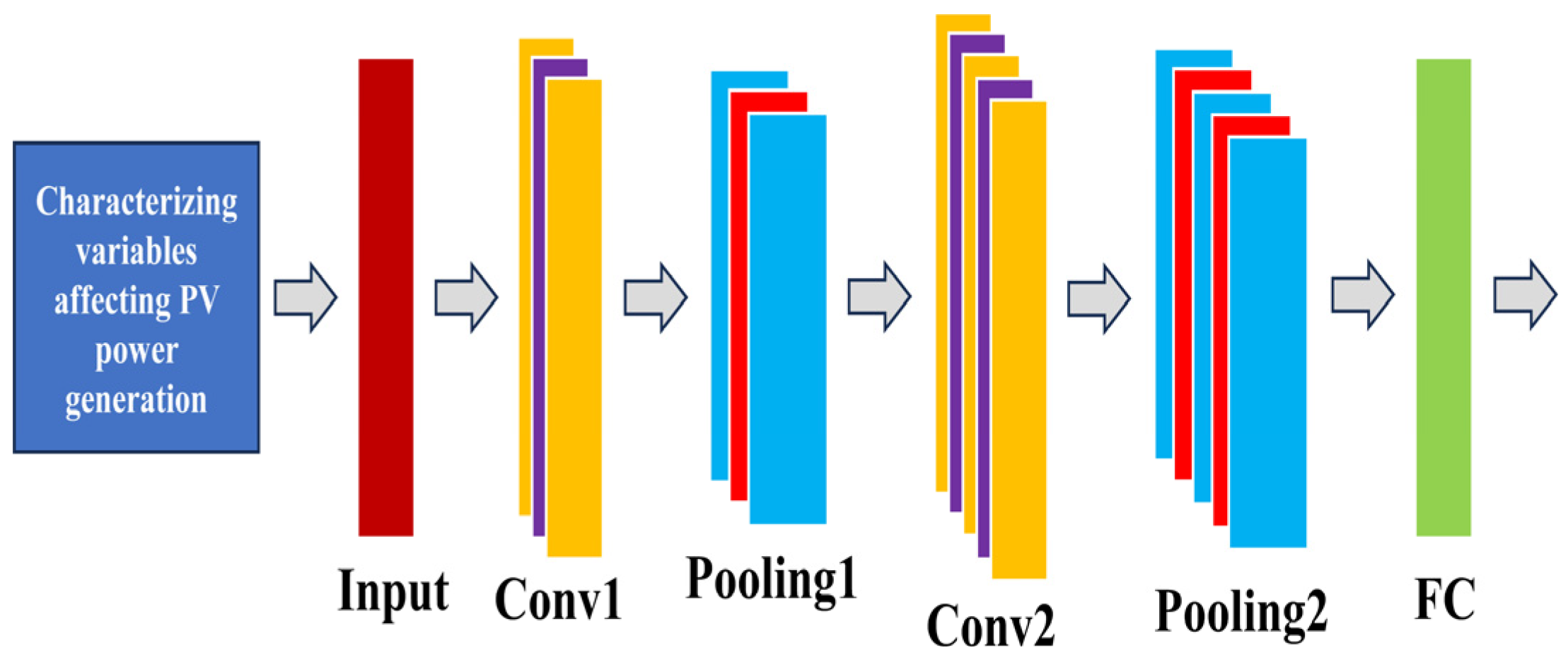
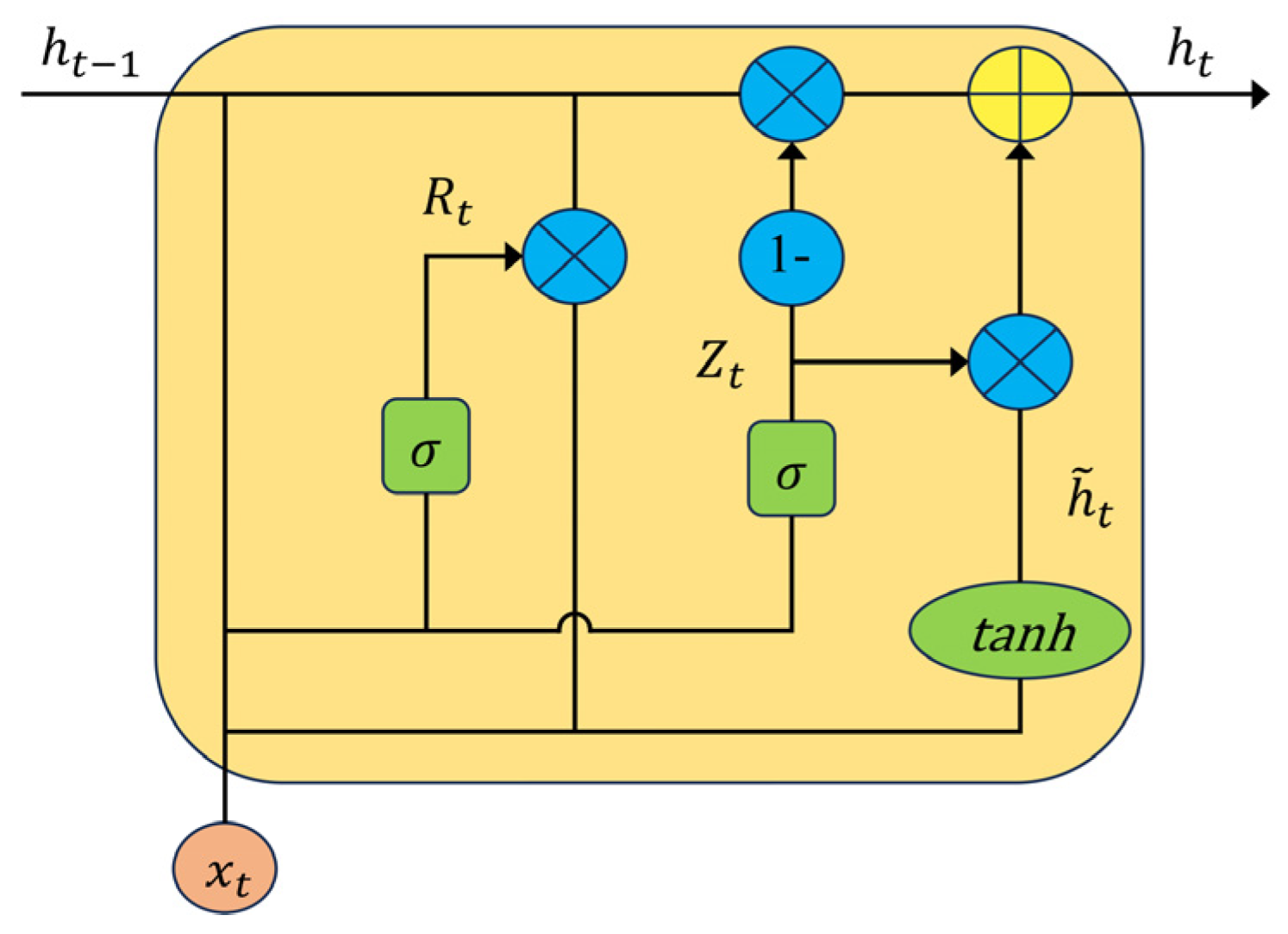
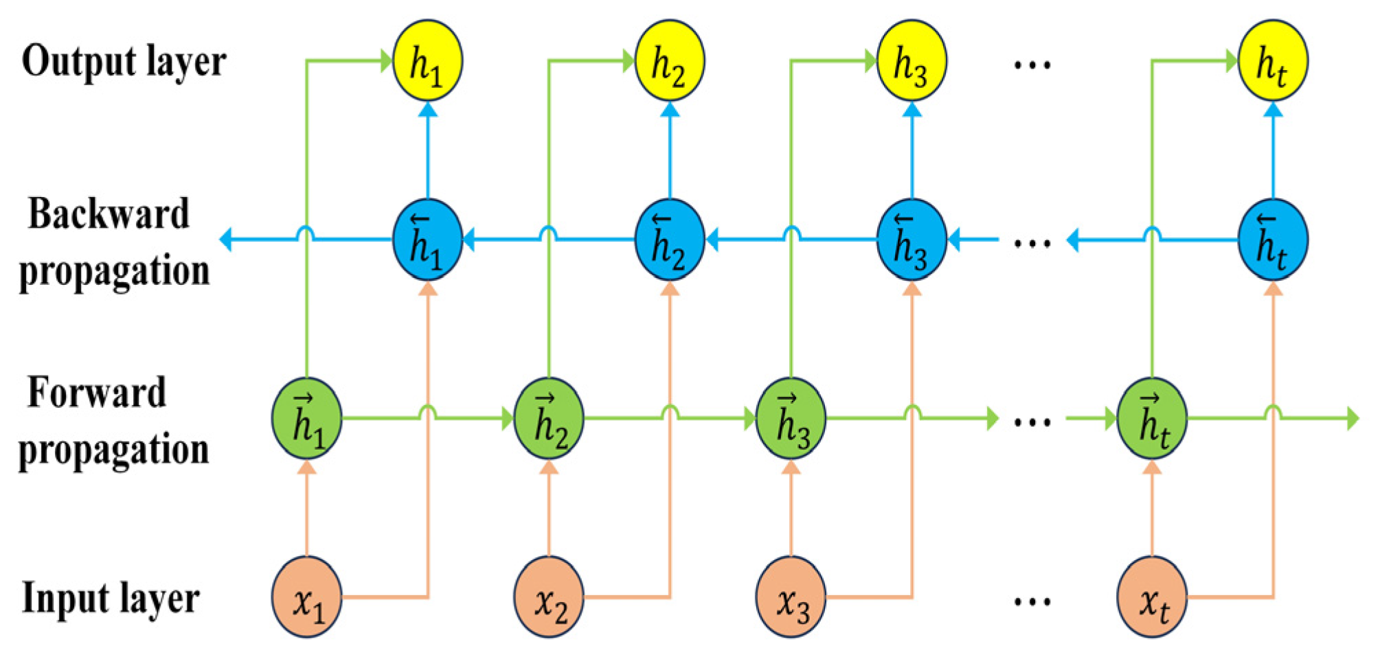
2.3.1. CNN-BIGRU

When it comes to data-feature extraction, the convolutional neural network (CNN) stands out as one of the most powerful methods. Traditionally employed in image processing and computer vision, CNNs have proven effective in capturing meaningful patterns. In this study, we utilize a one-dimensional convolutional neural network (1D-CNN) specifically designed for time-series data. Compared to two-dimensional and three-dimensional counterparts, the 1D-CNN demonstrates superior feature-extraction capabilities for time-series data. Its ability to filter out noise and uncover intricate relationships within the data allows for a deeper understanding of temporal dynamics. The CNN consists primarily of three key components: the convolution layer, the pooling layer, and the fully connected layer. These components are designed to effectively reduce model complexity and computational costs while enhancing model generalization and preventing overfitting. Weight sharing and local connection techniques play a vital role in achieving these objectives. The convolution layer serves to extract meaningful feature vectors from the input data, encompassing PV power generation and factors influencing power generation. This extraction is achieved by sliding a convolution kernel over the input, followed by activation through a modified linear unit (ReLU) and nonlinear mapping. Subsequently, the obtained features are passed to the pooling layer, which plays a crucial role in feature selection. By employing techniques such as average pooling or maximum pooling, the pooling layer retains the essential data features while reducing the dimensionality and simplifying the model. The output from the pooling layer is then forwarded to the fully connected layer, which ultimately produces the desired results in the output layer. In this study, we propose a model comprising two convolution layers and two maximum pooling layers, as illustrated in Figure 6. The mathematical modeling process is outlined as follows:

$$\left\{\begin{array}{c}{C}_1=f(x_t\odot W_1+b_1)\\ P_1=Max\left(C_1\right)+b_{2 }\\ \begin{array}{c}{C}_2=f(P_1\odot W_2+b_3)\\ P_2=Max\left(C_2\right)+b_{4 }\\ H_{FC}=f(P_2\odot W_3+b_5)\end{array}\end{array}\right.$$

(4)

where $x_t$ is the feature variable of the CNN input layer; $\odot$ stands for matrix operation; $C_1$ and $C_2$are the first and second convolutional layers, respectively; $P_1$ and $P_2$ are the first and second maximal pooling layers, respectively; $b$ and $W$ are the biases and weights of the corresponding layers; and $H_{FC}$ is the fully connected layer.

Once the data-feature information has been thoroughly mined, it is directly fed into the bidirectional gated recurrent unit (BIGRU) model for prediction. The data under investigation in this study falls into the category of time-series data. For processing such data, the recurrent neural network (RNN) proves advantageous due to its ability to retain memory. Unlike the feedforward neural network, the RNN incorporates connections between hidden-layer nodes, enabling it to effectively capture temporal dependencies. The hidden layer at the current moment can incorporate information from the hidden layer at the previous moment, allowing for the processing of input sequences in any time sequence. However, when dealing with long sequences, RNNs are susceptible to the issues of “gradient disappearance” and “gradient explosion”, necessitating limitations on the utilization of historical data. To address this challenge, the long short-term memory (LSTM) model was introduced. It consists of a main memory unit comprising a forgetting gate, an input gate, and an output gate. Nonetheless, the LSTM’s increased network complexity, higher parameter count, and slower convergence speed pose certain drawbacks. In contrast, the gated recurrent unit (GRU) represents an upgraded and simplified version of LSTM. Its memory unit features only a reset gate and an update gate, which effectively retains the memory function while significantly reducing training parameters. The GRU achieves faster processing speeds and proves highly efficient with large-scale sequence data, all at minimal computational cost, as depicted in Figure 7. The mathematical modeling process is detailed as follows:

$${ R}_t=\sigma \left(W_R{x}_t+U_R{h}_{t-1}+b_R\right)$$

(5)

$$Z_t=\sigma (W_Z{x}_t+U_Z{h}_{t-1}+b_Z)$$

(6)

$${\tilde{h}}_t=tanh\left(W_h{x}_t+R_t\odot U_h{h}_{t-1}+b_h\right)$$

(7)

$$h_t=\left(1-Z_t\right)\odot h_{t-1}+Z_t\odot {\tilde{h}}_t$$

(8)

where $x_t$ is the input variable at the current moment; $R_t$and $Z_t$ are the reset and update gates; $W$ and $U$ are the weights of the corresponding functions, and $b$ is the bias; $\sigma$ is the Sigmoid activation function; $\odot$ stands for the matrix operation; ${\tilde{h}}_t$ is the intermediate memory state; and $h_t$ and $h_{t-1}$ are the outputs at the current moment and the outputs at the previous moment.

RNN, LSTM, and GRU are limited to unidirectional propagation, flowing solely from past moments to future moments. However, predicting future PV power generation requires consideration of both historical and future meteorological data. In contrast, the BIGRU model comprises two GRUs that process sequence data bidirectionally, allowing information flow not only from historical data to future data but also from future data to historical data, as depicted in Figure 8. This model structure is advantageous for effective mining and utilizing deep feature information from both the preceding and subsequent data points, thereby enhancing the model’s generalization capability.

The output at time $t$ is $h_{t }$, which represents the sum of the output of the front and rear bidirectional hidden layers. The calculation formula is as follows:

$$\left\{\begin{array}{c}{\overleftarrow{h}}_t=GRU\left(x_t,{\overleftarrow{h}}_{t-1}\right)\\ {\overrightarrow{h}}_t=GRU\left(x_t,{\overrightarrow{h}}_{t-1}\right)\\ h_t=W{\overleftarrow{h}}_t+U{\overrightarrow{h}}_t+b_t\end{array}\right.$$

(9)

where: ${\overleftarrow{h}}_t$ and ${\overrightarrow{h}}_t$ are the backward and forward propagation, respectively, and GRU ($·$) represents the model’s arithmetic process.

2.3.2. POA

The pelican optimization algorithm (POA) was introduced by Trojovsky Pavel et al. in 2022 as a cutting-edge swarm-intelligence optimization algorithm known for its remarkable global search-optimization capability [48]. POA is inspired by the pelican-hunting method, and it establishes a mathematical model by simulating the process of pelicans capturing food. In this algorithm, each pelican’s position represents a candidate solution to the problem at hand. The solution and optimization processes are realized through the emulation of the pelican’s food-capture behavior. Similar to other swarm-intelligence optimization algorithms, the initialization of the population positions follows a standard approach, as shown in the following formula:

$$x_{i,j}=l_j+rand·\left(u_j-l_j\right), i=\mathrm{1,2},\dots ,D , j=\mathrm{1,2},\dots ,K.$$

(10)

where $x_{i,j}$ is the position of the $i$th pelican in the $j$th dimension; $D$ is the number of pelican populations; $K$ is the dimension of the solution problem; $rand$ is a random function that generates random numbers of [0,1]. $u_j$ and $l_j$ are the upper and lower bounds of the solution problem in the $j$th dimension, respectively.

Pelican population location distribution can be represented by the following matrix search space:

$$X=\left(\begin{array}{c}{X}_1 \\ ⋮\\ X_i\\ ⋮\\ X_D\end{array}\right)=\left(\begin{array}{c}\begin{array}{c}{x}_{\mathrm{1,1}}\\ ⋮\\ x_{i,1}\end{array}\\ ⋮\\ x_{D,1}\end{array}\begin{array}{c}\begin{array}{c}\dots \\ \ddots \\ \dots \end{array}\\ ⋰\\ \dots \end{array}\begin{array}{c}\begin{array}{c}{x}_{1,j}\\ ⋮\\ x_{i,j}\end{array}\\ ⋮\\ x_{D,j}\end{array}\begin{array}{c}\begin{array}{c}\dots \\ ⋰\\ \dots \end{array}\\ \ddots \\ \dots \end{array}\begin{array}{c}\begin{array}{c}{x}_{1,K}\\ ⋮\\ x_{i,K}\end{array}\\ ⋮\\ x_{D,K}\end{array} \right)$$

(11)

where $X_i$ is the search position of the $i$th pelican.

The objective function value of the pelican is computed by incorporating the objective function of the problem being solved. To determine the specific value of the objective function, the following equation can be employed.

$$F=\left(\begin{array}{c}{F}_1 \\ ⋮\\ F_i\\ ⋮\\ F_D\end{array}\right)=\left(\begin{array}{c}\begin{array}{c}F\left(X_1\right)\\ ⋮\\ F\left(X_i\right)\end{array}\\ ⋮\\ F\left(X_D\right)\end{array} \right)$$

(12)

where $F$ is the objective function vector of the pelican population; $F_i$ is the objective function value of the $i$th pelican.

Phase I is the flying to the prey (exploration phase).

Contrary to the behavior of other birds, pelicans exhibit a unique hunting strategy by swiftly flying towards the location of their spotted prey. By mathematically modeling this predatory approach, POA effectively scans the search space, leveraging its inherent capacity to explore various regions within this space. Notably, the prey’s location is randomly generated within the search space, thereby enhancing the algorithm’s exploratory capability in precisely identifying the problem’s solution. This process is mathematically represented as follows:

$$x_{i,j}^{P1}=\left\{\begin{array}{cc}{ x}_{i,j}+rand·\left(p_j-I·x_{i,j}\right),\hfill & \hfill F_p<F_i\\ x_{i,j}+rand·\left(x_{i,j}-p_j\right),\hfill & \hfill else\end{array}\right.$$

(13)

where $x_{i,j}^{P1}$ is the updated position of the $i$th pelican in the $j$th dimension; $p_j$ is the position of the prey in the $j$th dimension; $I$ is a random integer of 2 or 1, which is randomly generated at each iteration; and $F_p$ is the objective function value.

If the objective function value improves at a given position, indicating better problem-solving performance, the position is updated after accepting it. This efficient position-update method helps prevent the algorithm from searching in non-optimal regions. The formula for this update process is as follows:

$$X_i=\left\{\begin{array}{cc}{ X}_i^{P1},\hfill & \hfill F_i^{P1}<F_i\\ X_i,\hfill & \hfill else\end{array}\right.$$

(14)

where ${ X}_i^{P1}$ is the new position of the $i$th pelican; $F_i^{P1}$ is the value of the objective function after updating the position based on the first stage.

Phase II is surface flight (development phase).

Upon reaching the water where the fish are located, pelicans employ a distinctive hunting technique by flapping their wings to force the fish to swim upwards. Subsequently, they ensnare the fish within a capacious throat pouch. This capture method enables pelicans to efficiently accumulate a larger quantity of fish. By mathematically modeling this predatory behavior, POA enhances its convergence towards optimal positions and obtains improved problem solutions. Consequently, the search capability of the POA algorithm is enhanced. This process can be mathematically represented as follows:

$$x_{i,j}^{P2}={ x}_{i,j}+L·(1-t/T)·(2·rand-1)·{ x}_{i,j}$$

(15)

where $x_{i,j}^{P2}$ is the position of the $i$th pelican after updating in the $j$th dimension; $L=0.2$. The variable $t$ represents the current iteration number, while $T$ represents the maximum iteration number. The coefficient $L·(1-t/T)$ is the radius of the neighborhood of ${ x}_{i,j}$, which is searched in the vicinity of each member to get the local optimal solution and then aggregated to each local optimal solution to get the global optimal solution. During the initial iteration, this coefficient has a large value, resulting in a wide search region around each member. As the algorithm progresses, the coefficient gradually decreases, leading to a reduction in the radius of the search domain for each member. This iterative process enables the POA algorithm to effectively locate the best solution in close proximity to the global optimum. Notably, the effective update position method remains the same as in the first stage.

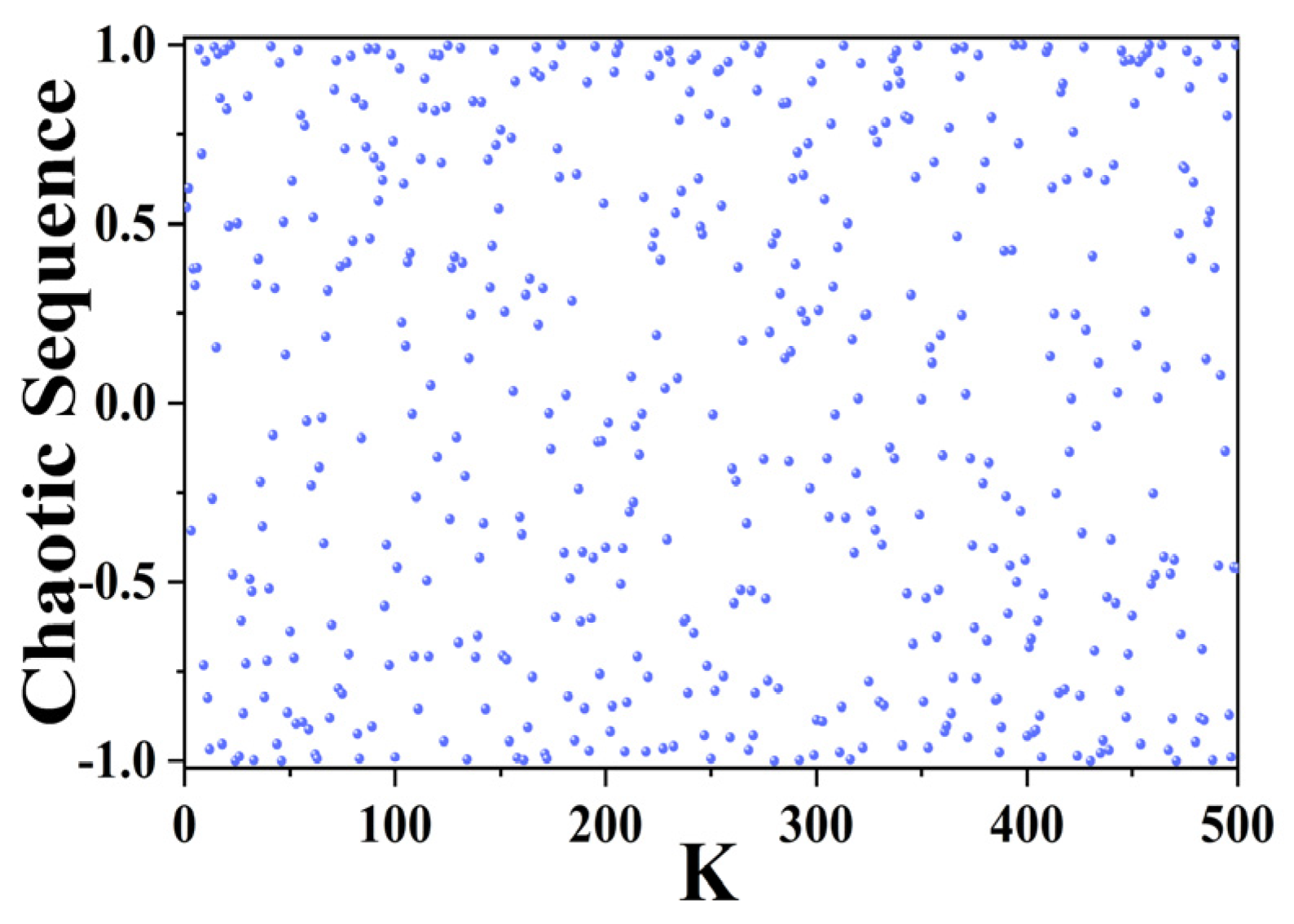
2.3.3. ICMIC Chaotic Mapping

The distribution of initial positions within the heuristic algorithm significantly impacts both the global optimization accuracy and convergence speed. However, the randomly generated initial population in the POA exhibits uneven distribution and low ergodicity, leading to suboptimal population quality. To address this limitation, this paper proposes the utilization of ICMIC mapping, a chaotic mapping technique, to generate the initial position of the pelican population. This approach greatly enhances the randomness of the initial population and facilitates the selection of individuals with superior fitness as the initial population. Consequently, the global search capability of the algorithm is enhanced, and the convergence speed is accelerated. The ICMIC chaotic mapping employed in this study is characterized by infinite folding times [49,50], making it more likely to exhibit chaotic phenomena compared to other maps with limited folding times. The mathematical expression for the ICMIC chaotic mapping is as follows:

$$X_k=\sin \left(\frac{\alpha }{x_{k-1}}\right)$$

(16)

where $x_k$ is the chaotic sequence generated by the mapping, $\alpha \in (0,+\infty )$. As in Figure 9, the chaotic sequence is generated by taking $\alpha$ = 100 and $k$ from 2 to 500; the chaos is more obvious.

2.4. CNN-BIGRU Prediction Model Based on ICMIC-POA

This paper introduces the ICMIC-POA-CNN-BIGRU prediction model, which consists of two components: the main prediction model (CNN-BIGRU) and the heuristic optimization algorithm model (ICMIC-POA). The selection of appropriate hyperparameters for the main prediction model plays a crucial role in ensuring robustness and prediction accuracy. However, traditional methods for hyperparameter optimization often require extensive manual debugging, resulting in high computational and time costs. In contrast, heuristic algorithms offer unique advantages in solving optimization problems and efficiently obtaining global optimal solutions. Figure 10 illustrates the prediction process of the overall prediction model proposed in this study, which can be expressed as follows:

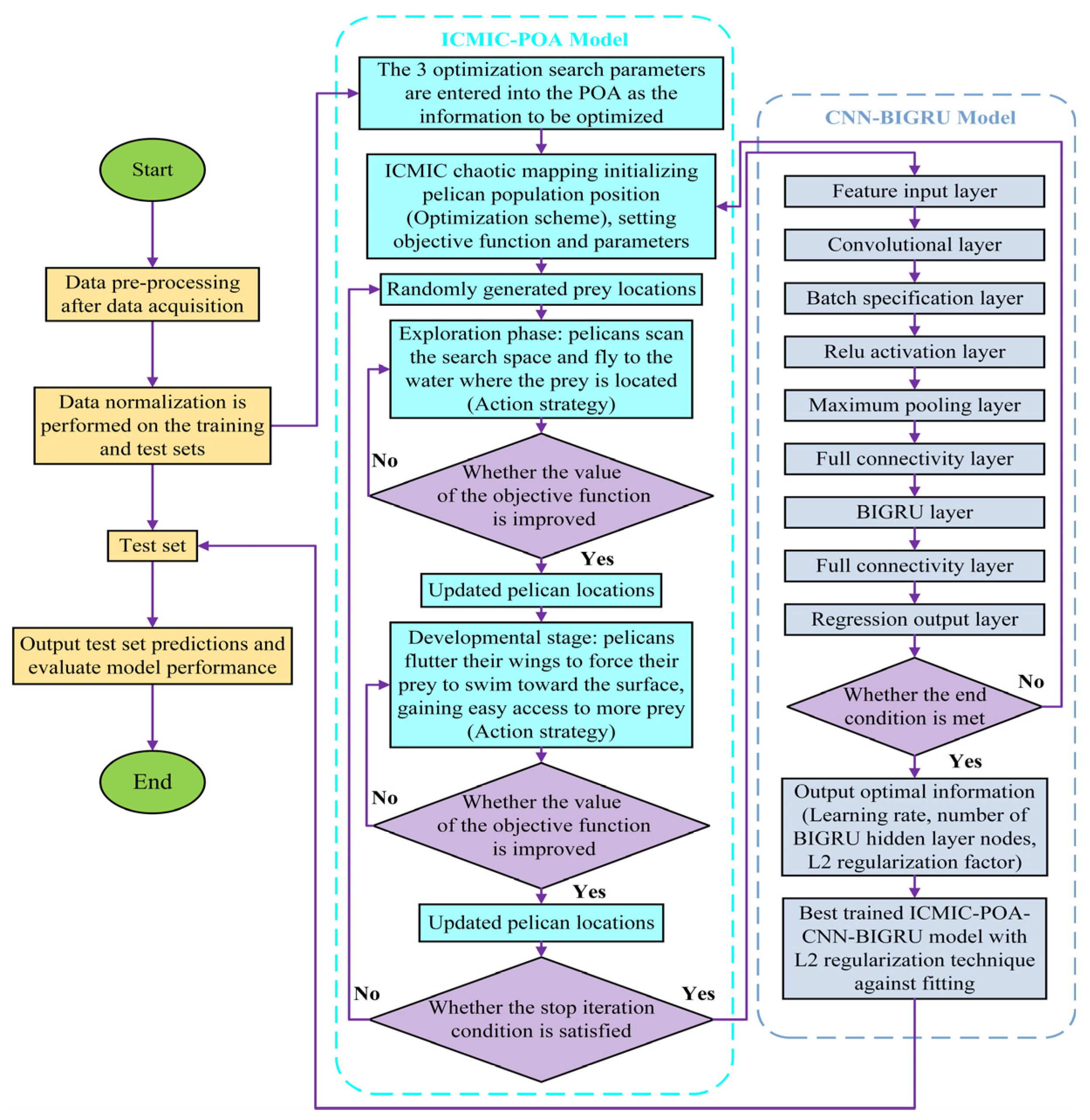
• The original dataset is partitioned into training and test sets, and the data is normalized;
• Three optimization search parameters are input into the POA as the variables to be optimized;
• The initialization of the pelican population’s position is carried out using the ICMIC chaotic mapping technique. In this study, the three parameters subject to optimization are the learning rate, the number of nodes in the hidden layer of the BIGRU, and the L2-regularization coefficient λ. The fitness function of the POA, which is the mean-square error, serves as the objective function, while the remaining parameters are set accordingly;
• Randomly generated prey locations;
• In the exploration phase, pelicans scan the search space and fly to the water where the prey is located (action strategy);
• The objective function of the exploration phase is worth improving and updating the pelican position. Otherwise, return to step (5);
• In the developmental stage, pelicans flutter their wings to force their prey to swim toward the surface, easily gaining more prey (action strategy);
• The objective function of the development phase is worth improving and updating the pelican position. Otherwise, return to step (7);
• Satisfy the stop iteration condition and output to the CNN-BIGRU model. Otherwise, return to step (4);
• CNN deep mines the features of time series variables and inputs them to BIGRU for prediction;
• After the end condition is satisfied, output the optimal 3 parameter values. Otherwise, return to step (3);
• The best-trained ICMIC-POA-CNN-BIGRU model for prediction and performance evaluation of the test set.

Among the neural networks utilized in this study, CNN demonstrates a robust ability to extract valuable feature information, while BIGRU, with its memory units, proves advantageous for time-series data prediction. These two networks exhibit excellent prediction performance even when operating with a limited dataset. It is important to note that employing a large dataset significantly increases the computational burden of the model in this study. Therefore, for the purpose of short-term prediction, a smaller dataset spanning two months is employed. However, it is acknowledged that using a small dataset may lead to issues such as overfitting or poor generalization. To address these challenges, the L2-regularization technique is employed. In comparison to other regularization methods, L2 regularization effectively mitigates overfitting without sacrificing valuable feature information. By incorporating regular terms into the objective function, L2 regularization penalizes model complexity and facilitates the development of a simpler model with fewer parameters. The calculation formula for L2 regularization is as follows:

$$J\left(w,x,y\right)=L\left(w,x,y\right)+\frac{\lambda }{2}{w}^{T}w$$

(17)

where $L\left(w,x,y\right)$ is the objective function before regularization and $J\left(w,x,y\right)$ is the objective function after regularization. $\frac{\lambda }{2}{w}^{T}w$ is the L2 regular term, which mainly changes the size of the weights $w$ through the regularization coefficient $\lambda$ to achieve the anti-fitting effect.

3. Result and Discussion

3.1. Evaluation Index

In this paper, the determination coefficient $R^2$, mean absolute error (MAE), mean absolute percentage error (MAPE), mean bias error (MBE), mean square error (MSE), and root mean square error (RMSE) were used as the evaluation indexes of model performance. The formula is as follows:

$$R^2=1-\frac{{\sum }_{i=1}^N{(W_{forecasting}-W_{true})}^2}{{\sum }_{i=1}^N{(W_{true}-{\overline{W}}_{true})}^2}$$

(18)

$$MAE=\frac{1}{N}{\sum }_{i=1}^N\left|W_{forecasting}-W_{true}\right|$$

(19)

$$MAPE=\frac{1}{N}{\sum }_{i=1}^N\left|\frac{W_{forecasting}-W_{true}}{W_{true}}\right|\times 100\%$$

(20)

$$MBE=\frac{1}{N}{\sum }_{i=1}^N(W_{forecasting}-W_{true})$$

(21)

$$MSE=\frac{1}{N}{\sum }_{i=1}^N{\left(W_{forecasting}-W_{true}\right)}^2$$

(22)

$$RMSE=\sqrt{\frac{1}{N}\left({\sum }_{i=1}^N{\left(W_{forecasting}-W_{true}\right)}^2\right)}$$

(23)

where $N$ is the number of samples; $W_{true}$ is the actual power-generation value; $W_{forecasting}$ is the predicted value; and ${\overline{W}}_{true}$ is the average of all actual values.

3.2. Prediction Results and Analysis

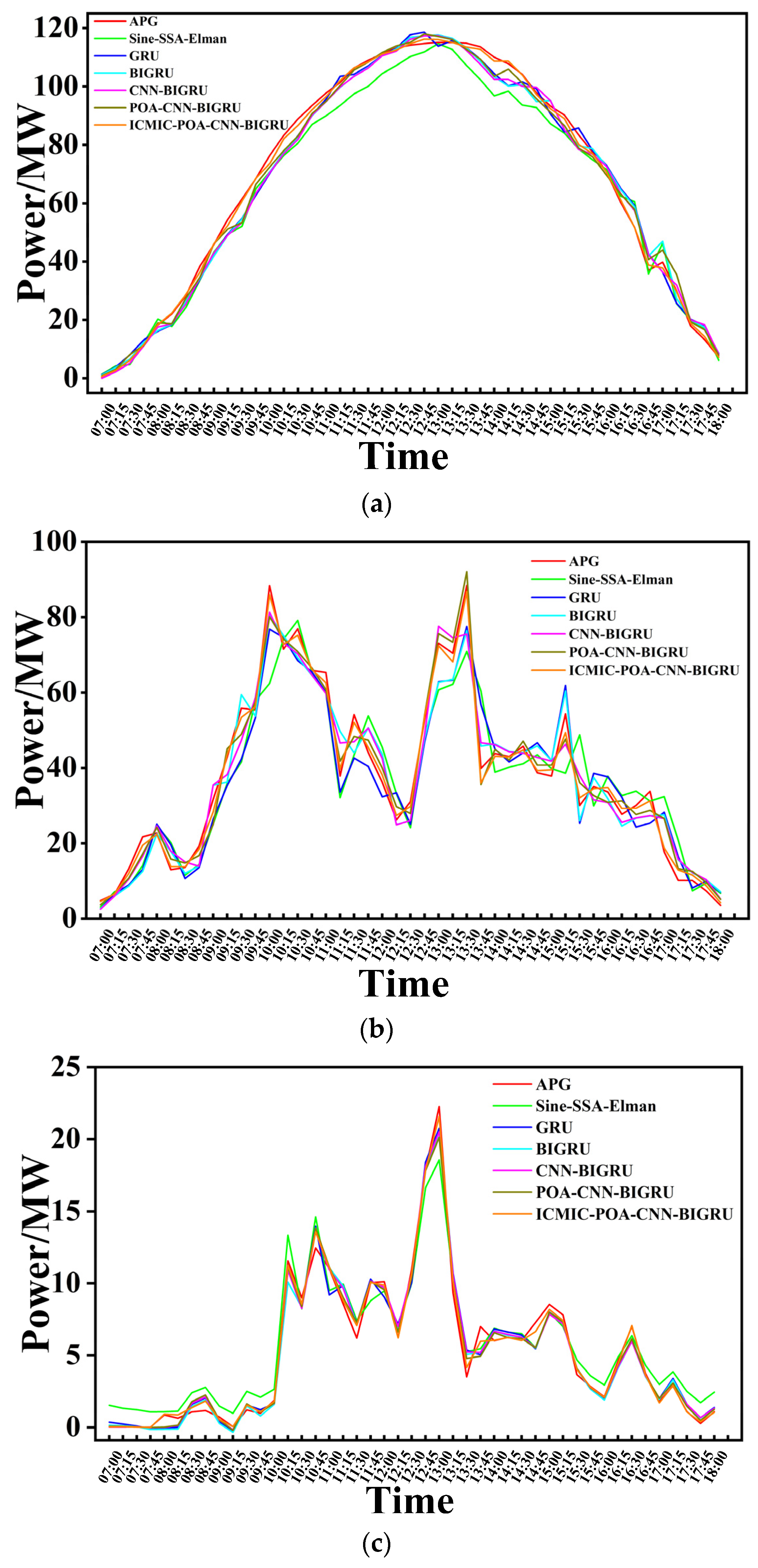
3.2.1. Prediction of Three Typical Days

To effectively evaluate the performance of the proposed prediction model, this study randomly selects three representative days (sunny, cloudy, and rainy) as the test set, with a prediction time window of one day. The remaining data were utilized as the training set.

Table 1. Model structural parameters.

Structural Parameter	Parameter Value	Structural Parameter	Parameter Value
Number of pelican populations	20	Number of convolution kernels in the first layer	16
The maximum number of iterations of POA	50	Convolution layer activation function	ReLU
Single-batch processing samples	128	The second-layer convolution kernel size and step size	4.1
Maximum training iterations	300	Number of convolution kernels in the second layer	32
Optimizer	Adam	Pooling size and step size	2.1
The first-layer convolution kernel size and step size	3.1	BIGRU activation function	Tanh

presents the detailed structural parameters of the prediction model, encompassing the population size for the heuristic optimization algorithm, the maximum number of iterations for POA, the maximum training iterations for the deep learning model, and other relevant parameters. These parameters need to be set prior to initiating the training process, followed by training and validation, and ultimately testing. The workstation configuration on which the experiment was run was Windows 10 Professional Workstation Edition, RAM 256GB, Intel(R) Xeon(R) Gold 6252 [email protected] 2.10GHz (two processors), and NVIDIA Quadro RTX 6000.

Figure 11 illustrates the evolutionary convergence of the optimal fitness for both the ICMIC-POA and POA algorithms in predicting three representative days. The fitness function employed in this analysis was MSE. The results demonstrated that the convergence speed and fitness values varied across different weather types. However, it was noteworthy that the pelican population, initialized using the ICMIC chaotic mapping technique, exhibited faster convergence speed and lower fitness values compared to the population without optimization. This indicated that the ICMIC chaotic mapping effectively enhanced the randomness, distribution uniformity, and ergodicity of the pelican population’s position. As a result, the optimization speed of POA was significantly accelerated, and its global search ability was strengthened.

The loss function plays a pivotal role in training the deep learning model. It aims to minimize the discrepancy between the predicted values and the actual values by reducing the loss on the training set. This iterative process leads to continuous improvement in the performance of the prediction model and enhances its generalization ability on the test set. In this study, the MSE was employed as the loss function. Figure 12 compares the loss values before and after incorporating L2-regularization technology for three representative days, using 150 training iterations as an example. Specifically, Figure 12a,c,e depict the loss curves without L2-regularization technology. As the number of training iterations increases, the loss value exhibits a slow decrease, and the loss value of the validation set surpasses that of the training set, indicating the presence of overfitting. Moreover, the loss curve displays a wide range of fluctuations. Consequently, the generalization ability of the model trained under these circumstances cannot be guaranteed. In contrast, Figure 12b,d,f illustrate the loss curves obtained when employing the L2-regularization technique. Notably, as the training progresses, the loss value rapidly decreases, and the loss value of the verification part is not higher than that of the training part. Additionally, the loss curve converges quickly within a narrow range of volatility, significantly enhancing the model’s stability. These findings strongly supported the notion that incorporating L2-regularization technology effectively counteracted overfitting and improved the model’s generalization ability.

To comprehensively assess the prediction performance of the proposed model, a comparative analysis is conducted with several other models, namely Sine-SSA-Elman (where Sine represents a chaotic mapping, SSA refers to the sparrow-search algorithm, and Elman represents a neural network algorithm), GRU, BIGRU, CNN-BIGRU, and POA-CNN-BIGRU. A total of 20 experiments were performed, utilizing six evaluation metrics for performance assessment. Figure 13, Figure 14 and Figure 15 show the prediction effects of different prediction models on sunny, cloudy, and rainy days, respectively. The size of the box in the box-and-line plot indicates the distribution of the assessment metrics, and a colored dot indicates the assessment value corresponding to one experiment. The horizontal line inside the box indicates the average value of 20 experiments for each model and is displayed on the right side of the box. The larger the value of the regression fit coefficient $R^2$, the better the prediction. The closer the MBE value is to 0, the better the prediction. The smaller the value of the other four assessments, the better the prediction. The findings reveal that among the three typical day forecasts, the model proposed in this paper has the best six evaluation indexes and the smallest error fluctuation range, indicating that the prediction effect is better than the other five models, and it is able to make effective PV power prediction for different weather with the best robustness and generalization ability. Specifically, the proposed model achieved the average value of $R^2$ of 0.98372 for a sunny day, 0.97589 for a cloudy day, and 0.98735 for a rainy day. In contrast, the best $R^2$ mean for the Sine-SSA-Elman model was 0.9192 on a sunny day and 0.86063 in cloudy weather, with a wide range of fluctuations. It was worth noting that the model proposed in this paper could reduce the mean value of MSE to 0.06398 MW and the mean value of MAE to 0.19368 MW during rainy weather prediction. In cloudy weather prediction, which has the most fluctuating power of PV, the mean value of RMSE could be reduced to 3.73881 MW and the mean value of MAE could be reduced to 2.99258 MW. This indicated that the model had strong generalization ability and high accuracy performance. In order to observe the prediction effect of different weather more intuitively, Figure 16 shows the prediction effect of the six prediction models on three typical days.

Table 2. ICMIC-POA search for optimal values of 3 parameters.

Number of Experiments	Optimal number of Hidden Layer Nodes for BIGRU	Optimal Initial Learning Rate	Optimal L2-Regularization Factor
	Range [10,135]	Range [0.001,0.01]	Range [0.0001,0.1]
1	85	0.0028	0.0014
2	90	0.0051	0.0056
3	23	0.0078	0.0067
4	118	0.0071	0.0060
5	21	0.0021	0.0052
6	116	0.0039	0.0024
7	121	0.0038	0.0089
8	116	0.0051	0.0122
9	37	0.0070	0.0019
10	30	0.0045	0.0054
11	19	0.0020	0.0039
12	98	0.0043	0.0212
13	23	0.0089	0.0077
14	91	0.0081	0.0267
15	95	0.0076	0.0256
16	75	0.0036	0.0081
17	45	0.0021	0.0068
18	52	0.0095	0.0165
19	96	0.0061	0.0136
20	95	0.0067	0.0076

provides a comprehensive overview of the ICMIC-POA experiments, showcasing the automatic iteration process to identify the three optimal initial parameter values for CNN-BIGRU during the prediction of power generation in cloudy weather. Notably, this study maintains uniformity by setting the number of nodes in the two hidden layers of BIGRU to be equal.

3.2.2. K-Fold Cross-Validation

The prediction time window for the three representative days was set to one day, with consistent training and test data across the 20 experiments. While this approach reduces the variability in evaluating the model’s prediction performance on the same dataset, it does not assess the model’s ability to predict different datasets. To address this limitation and comprehensively assess the robustness and generalization ability of the prediction model, this study employs K-fold cross-validation, which effectively mitigates this concern. It is important to highlight that this method is particularly useful for small-sample datasets and can also help mitigate overfitting. After data processing, the effective data group from the original dataset consisted of a total of 56 days. This study employed a K value of 17, resulting in the division of the 51-day dataset into 17 sub-datasets for cross-validation. Each sub-dataset served as an individual test set, with a prediction time window of 3 days. Consequently, a total of 17 cross-validations were conducted. Furthermore, when extending the prediction time window to 5 days, a K value of 10 was selected, dividing the 50-day dataset into 10 sub-datasets for 10 cross-validations. The evaluation index chosen in this study was the RMSE, which facilitated a comparison of the prediction performance among three hybrid models: ICMIC-POA-CNN-BIGRU, POA-CNN-BIGRU, and CNN-BIGRU. The results, presented in

Table 3. RMSE values of different models for 3 consecutive days were predicted.

Prediction Intervals	Assessment Indicators	Forecasting Models
		ICMIC-POA-CNN-BIGRU	POA-CNN-BIGRU	CNN-BIGRU
3 Days	RMSE/MW	2.8949	4.8083	5.1422
		1.3377	3.3137	4.3971
		2.8195	4.4362	5.5421
		2.3524	5.0615	4.9599
		1.2879	3.3776	3.6108
		2.0072	5.3213	6.1252
		0.9581	2.9286	3.1163
		1.2262	3.7977	5.4232
		1.6176	3.6883	4.2821
		1.4799	3.9245	5.6274
		0.8723	2.1958	4.9951
		3.8364	5.6568	5.8586
		3.3353	5.8328	6.1136
		1.3593	3.1487	5.5886
		1.6912	3.8669	5.3778
		2.8984	4.4009	5.9135
		2.8831	4.5222	6.4113
	Mean value	2.0504	4.1342	5.2050

and

Table 4. RMSE values of different models for 5 consecutive days were predicted.

Prediction Intervals	Assessment Indicators	Forecasting Models
		ICMIC-POA-CNN-BIGRU	POA-CNN-BIGRU	CNN-BIGRU
5 Days	RMSE/MW	2.9281	3.5113	4.0149
		3.4851	5.0503	5.6674
		2.2264	4.3259	5.3498
		2.7534	3.7559	4.9186
		5.0063	6.2719	7.1561
		3.3317	4.8321	5.0249
		3.6894	4.9451	5.4569
		4.1103	5.4777	6.2314
		5.4194	6.6264	5.4731
		3.3508	4.7218	5.7427
	Mean value	3.6301	4.9518	5.5036

, indicate that the ICMIC-POA-CNN-BIGRU model proposed in this paper outperformed the other two hybrid models, exhibiting the smallest fluctuation range in RMSE.

To provide a detailed comparison of the prediction effects across different prediction time windows (1 day, 3 days, and 5 days), we have compiled the average value of the RMSE evaluation index from our previous experiments, as illustrated in Figure 17. The results demonstrate that the model proposed in this study consistently achieved the lowest RMSE value in predicting various weather conditions and different prediction time windows, indicating its superior prediction performance. Especially on rainy days, the RMSE value could be reduced to 0.2517 MW, which was 57.59% lower than the RMSE value of the CNN-BIGRU model. On sunny and cloudy days, the RMSE values of the proposed model were 64.08% and 46.14% lower than those of the CNN-BIGRU model, respectively. In the prediction time window of 3 days and 5 days, the RMSE values of the model proposed in this paper were reduced by 60.61% and 34.04%, respectively, compared with the CNN-BIGRU model. It was worth noting that, in the ICMIC-POA-CNN-BIGRU and CNN-BIGRU models, the RMSE value of the predicted 5 days was larger than that of the predicted 3 days and the predicted sunny and rainy days but was smaller than the predicted cloudy days. In the POA-CNN-BIGRU model, the RMSE value of the predicted 5 days was the largest. This shows that, when the same model predicts different prediction time windows, the longer the prediction time window, the prediction performance is not necessarily worse. Figure 18a,b visually show the prediction of the above model in the prediction time window of 3 days and 5 days, respectively. The results show that the prediction effect of the model proposed in this paper was better than the other two prediction models at the peak and trough. This is conducive to the stable operation of the PV power-generation system and reduces the impact on the power grid, bringing good economic benefits to the PV station.

4. Conclusions

This paper introduced a high-performing hybrid model designed to address the challenge of short-term power-output prediction in new island PV stations operating under high humidity conditions. The proposed model holds significant potential in facilitating the efficient utilization of abundant coastal PV resources and promoting the rapid development of this emerging category of island PV stations. Additionally, it offers cost-saving benefits by reducing the maintenance expenses associated with PV stations, while also generating substantial economic gains. This is conducive to the sustainability of new energy generation and power systems. The main conclusions drawn from this research are summarized below.

• The latest heuristic algorithm (POA) was used for the first time to search and automatically debug the optimal hyperparameters of CNN-BIGRU and the optimal value of the L2-regularization coefficient, which greatly saved the computational cost and improved the prediction performance of the model;
• ICMIC chaotic mapping optimized the initial population position of the POA, increased the randomness of the population distribution, and greatly improved the ergodicity and global search ability of the POA;
• Adding L2-regularization technology could quickly reduce the loss value of the loss function in the deep learning model (CNN-BIGRU), and the convergence was stable in a very small range. It solved the over-fitting problem that easily occurred in the training process;
• The model in this paper had the best prediction performance compared with the five prediction models. In the prediction time window of 1 day (sunny, cloudy, and rainy days), 3 days, and 5 days, six evaluation indicators were used to comprehensively evaluate the prediction performance.

References

1. Houran, M.A.; Bukhari, S.M.S.; Zafar, M.H.; Mansoor, M.; Chen, W. COA-CNN-LSTM: Coati optimization algorithm-based hybrid deep learning model for PV/wind power forecasting in smart grid applications. Appl. Energy 2023, 349, 121638. [Google Scholar] [CrossRef]
2. Agga, A.; Abbou, A.; Labbadi, M.; Houm, Y.E. Short-term self consumption PV plant power production forecasts based on hybrid CNN-LSTM, ConvLSTM models. Renew. Energy 2021, 177, 101–112. [Google Scholar] [CrossRef]
3. Micheli, L.; Talavera, D.L. Economic feasibility of floating photovoltaic power plants: Profitability and competitiveness. Renew. Energy 2023, 211, 607–616. [Google Scholar] [CrossRef]
4. Micheli, L.; Talavera, D.L.; Tina, G.M.; Almonacid, F.; Fernández, E.F. Techno-economic potential and perspectives of floating photovoltaics in Europe. Sol. Energy 2022, 243, 203–214. [Google Scholar] [CrossRef]
5. Bhattacharya, S.; Goswami, A.; Sadhu, P.K. Design, development and performance analysis of FSPV system for powering sustainable energy based mini micro-grid. Microsyst. Technol. 2023, 29, 1465–1478. [Google Scholar] [CrossRef] [PubMed]
6. Wang, J.; Zhou, Y.; Li, Z. Hour-ahead photovoltaic generation forecasting method based on machine learning and multi objective optimization algorithm. Appl. Energy 2022, 312, 118725. [Google Scholar] [CrossRef]
7. Pierro, M.; Gentili, D.; Liolli, F.R.; Cornaro, C.; Moser, D.; Betti, A.; Moschella, M.; Collino, E.; Ronzio, D.; van der Meer, D. Progress in regional PV power forecasting: A sensitivity analysis on the Italian case study. Renew. Energy 2022, 189, 983–996. [Google Scholar] [CrossRef]
8. Markovics, D.; Mayer, M.J. Comparison of machine learning methods for photovoltaic power forecasting based on numerical weather prediction. Renew. Sustain. Energy Rev. 2022, 161, 112364. [Google Scholar] [CrossRef]
9. Lauria, D.; Mottola, F.; Proto, D. Caputo derivative applied to very short time photovoltaic power forecasting. Appl. Energy 2022, 309, 118452. [Google Scholar] [CrossRef]
10. Alassery, F.; Alzahrani, A.; Khan, A.I.; Irshad, K.; Islam, S. An artificial intelligence-based solar radiation prophesy model for green energy utilization in energy management system. Sustain. Energy Technol. Assess. 2022, 52, 102060. [Google Scholar] [CrossRef]
11. Wang, Y.; Shen, R.; Ma, M. Research on ultra-short term forecasting technology of wind power output based on various me-teorological factors. Energy Rep. 2022, 8, 1145–1158. [Google Scholar] [CrossRef]
12. Fadhel, S.; Diallo, D.; Delpha, C.; Migan, A.; Bahri, I.; Trabelsi, M.; Mimouni, M.F. Maximum power point analysis for partial shading detection and identification in photovoltaic systems. Energy Convers. Manag. 2020, 224, 113374. [Google Scholar] [CrossRef]
13. Jia, P.; Zhang, H.; Liu, X.; Gong, X. Short-Term Photovoltaic Power Forecasting Based on VMD and ISSA-GRU. IEEE Access 2021, 9, 105939–105950. [Google Scholar] [CrossRef]
14. Niu, D.; Wang, K.; Sun, L.; Wu, J.; Xu, X. Short-term photovoltaic power generation forecasting based on random forest feature selection and CEEMD: A case study. Appl. Soft Comput. 2020, 93, 106389. [Google Scholar] [CrossRef]
15. Wang, L.; Liu, Y.; Li, T.; Xie, X.; Chang, C. The Short-Term Forecasting of Asymmetry Photovoltaic Power Based on the Feature Extraction of PV Power and SVM Algorithm. Symmetry 2020, 12, 1777. [Google Scholar] [CrossRef]
16. Hajjaj, C.; Ydrissi, M.E.; Azouzoute, A.; Oufadel, A.; Alani, O.E.; Boujoudar, M.; Abraim, M.; Ghennioui, A. Comparing Pho-tovoltaic Power Prediction: Ground-Based Measurements vs. Satellite Data Using an ANN Model. IEEE J. Photovolt. 2023, 13, 998–1006. [Google Scholar] [CrossRef]
17. Drałus, G.; Mazur, D.; Kusznier, J.; Drałus, J. Application of Artificial Intelligence Algorithms in Multilayer Perceptron and Elman Networks to Predict Photovoltaic Power Plant Generation. Energies 2023, 16, 6697. [Google Scholar] [CrossRef]
18. Ma, W.; Chen, Z.; Zhu, Q. Ultra-Short-Term Forecasting of Photo-Voltaic Power via RBF Neural Network. Electronics 2020, 9, 1717. [Google Scholar] [CrossRef]
19. Bozorg, M.; Bracale, A.; Carpita, M.; de Falco, P.; Mottola, F.; Proto, D. Bayesian bootstrapping in real-time probabilistic pho-tovoltaic power forecasting. Sol. Energy 2021, 225, 577–590. [Google Scholar] [CrossRef]
20. Wang, H.; Liu, Y.; Zhou, B.; Li, C.; Cao, G.; Voropai, N.; Barakhtenko, E. Taxonomy research of artificial intelligence for de-terministic solar power forecasting. Energy Convers. Manag. 2020, 214, 112909. [Google Scholar] [CrossRef]
21. Pan, M.; Li, C.; Gao, R.; Huang, Y.; You, H.; Gu, T.; Qin, F. Photovoltaic power forecasting based on a support vector machine with improved ant colony optimization. J. Clean. Prod. 2020, 277, 123948. [Google Scholar] [CrossRef]
22. Netsanet, S.; Dehua, Z.; Wei, Z.; Teshager, G. Short-term PV power forecasting using variational mode decomposition integrated with Ant colony optimization and neural network. Energy Rep. 2022, 8, 2022–2035. [Google Scholar] [CrossRef]
23. Ma, X.; Zhang, X. A short-term prediction model to forecast power of photovoltaic based on MFA-Elman. Energy Rep. 2022, 8, 495–507. [Google Scholar] [CrossRef]
24. Ge, L.; Xian, Y.; Yan, J.; Wang, B.; Wang, Z. A Hybrid Model for Short-term PV Output Forecasting Based on PCA-GWO-GRNN. J. Mod. Power Syst. Clean Energy 2020, 8, 1268–1275. [Google Scholar] [CrossRef]
25. Wang, H.; Lei, Z.; Zhang, X.; Zhou, B.; Peng, J. A review of deep learning for renewable energy forecasting. Energy Convers. Manag. 2019, 198, 111799. [Google Scholar] [CrossRef]
26. Huang, Y.; Wang, A.; Jiao, J.; Xie, J.; Chen, H. Short-Term PV Power Forecasting Based on CEEMDAN and Ensemble DeepTCN. IEEE Trans. Instrum. Meas. 2023, 27. [Google Scholar] [CrossRef]
27. Dairi, A.; Harrou, F.; Sun, Y.; Khadraoui, S. Short-Term Forecasting of Photovoltaic Solar Power Production Using Variational Auto-Encoder Driven Deep Learning Approach. Appl. Sci. 2020, 10, 8400. [Google Scholar] [CrossRef]
28. Mishra, S.P.; Rayi, V.K.; Dash, P.K.; Bisoi, R. Multi-objective auto-encoder deep learning-based stack switching scheme for improved battery life using error prediction of wind-battery storage microgrid. Int. J. Energy Res. 2021, 45, 20331–20355. [Google Scholar] [CrossRef]
29. Massaoudi, M.; Abu-Rub, H.; Refaat, S.S.; Trabelsi, M.; Chihi, I.; Oueslati, F.S. Enhanced Deep Belief Network Based on Ensemble Learning and Tree-Structured of Parzen Estimators: An Optimal Photovoltaic Power Forecasting Method. IEEE Access 2021, 9, 150330–150344. [Google Scholar] [CrossRef]
30. Chang, G.W.; Lu, H.-J. Integrating Gray Data Preprocessor and Deep Belief Network for Day-Ahead PV Power Output Forecast. IEEE Trans. Sustain. Energy 2020, 11, 185–194. [Google Scholar] [CrossRef]
31. Akhter, M.N.; Mekhilef, S.; Mokhlis, H.; Ali, R.; Usama, M.; Muhammad, M.A.; Khairuddin, A.S.M. A hybrid deep learning method for an hour ahead power output forecasting of three different photovoltaic systems. Appl. Energy 2022, 307, 118185. [Google Scholar] [CrossRef]
32. Garip, Z.; Ekinci, E.; Alan, A. Day-ahead solar photovoltaic energy forecasting based on weather data using LSTM networks: A comparative study for photovoltaic (PV) panels in Turkey. Electr. Eng. 2023, 105, 3329–3345. [Google Scholar] [CrossRef]
33. Zhang, Y.; Wang, Y. A Hybrid Neural Network-Based Intelligent Forecasting Approach for Capacity of Photovoltaic Electricity Generation. J. Circuits Syst. Comput. 2023, 32, 2350172. [Google Scholar] [CrossRef]
34. Li, Q.; Zhang, X.; Ma, T.; Liu, D.; Wang, H.; Hu, W. A Multi-step ahead photovoltaic power forecasting model based on TimeGAN, Soft DTW-based K-medoids clustering, and a CNN-GRU hybrid neural network. Energy Rep. 2022, 8, 10346–10362. [Google Scholar] [CrossRef]
35. Suresh, V.; Janik, P.; Rezmer, J.; Leonowicz, Z. Forecasting Solar PV Output Using Convolutional Neural Networks with a Sliding Window Algorithm. Energies 2020, 13, 723. [Google Scholar] [CrossRef]
36. Sajjad, M.; Khan, Z.A.; Ullah, A.; Hussain, T.; Ullah, W.; Lee, M.Y.; Baik, S.W. A Novel CNN-GRU-Based Hybrid Approach for Short-Term Residential Load Forecasting. IEEE Access 2020, 8, 143759–143768. [Google Scholar] [CrossRef]
37. Sabri, N.M.; Hassouni, M.E. Accurate photovoltaic power prediction models based on deep convolutional neural networks and gated recurrent units. Energy Source Part A 2022, 44, 6303–6320. [Google Scholar] [CrossRef]
38. Wang, F.; Xuan, Z.; Zhen, Z.; Li, K.; Wang, T.; Shi, M. A day-ahead PV power forecasting method based on LSTM-RNN model and time correlation modification under partial daily pattern prediction framework. Energy Convers. Manag. 2020, 212, 112766. [Google Scholar] [CrossRef]
39. Limouni, T.; Yaagoubi, R.; Bouziane, K.; Guissi, K.; Baali, E.H. Accurate one step and multistep forecasting of very short-term PV power using LSTM-TCN model. Renew. Energy 2023, 205, 1010–1024. [Google Scholar] [CrossRef]
40. Fan, T.; Sun, T.; Liu, H.; Xie, X.; Na, Z. Spatial-Temporal Genetic-Based Attention Networks for Short-Term Photovoltaic Power Forecasting. IEEE Access 2021, 9, 138762–138774. [Google Scholar] [CrossRef]
41. Zhou, Y.; Zhou, N.; Gong, L.; Jiang, M. Prediction of photovoltaic power output based on similar day analysis, genetic algorithm and extreme learning machine. Energy 2020, 204, 117894. [Google Scholar] [CrossRef]
42. Zhen, H.; Niu, D.; Wang, K.; Shi, Y.; Ji, Z.; Xu, X. Photovoltaic power forecasting based on GA improved Bi-LSTM in microgrid without meteorological information. Energy 2021, 231, 120908. [Google Scholar] [CrossRef]
43. Eseye, A.T.; Zhang, J.; Zheng, D. Short-term photovoltaic solar power forecasting using a hybrid Wavelet-PSO-SVM model based on SCADA and Meteorological information. Renew. Energy 2018, 118, 357–367. [Google Scholar] [CrossRef]
44. Perera, M.; De Hoog, J.; Bandara, K.; Halgamuge, S. Multi-resolution, multi-horizon distributed solar PV power forecasting with forecast combinations. Expert Syst. Appl. 2022, 205, 117690. [Google Scholar] [CrossRef]
45. Wu, X.; Lai, C.S.; Bai, C.; Lai, L.L.; Zhang, Q.; Liu, B. Optimal Kernel ELM and Variational Mode Decomposition for Probabilistic PV Power Prediction. Energies 2020, 13, 3592. [Google Scholar] [CrossRef]
46. Luo, L.; Abdulkareem, S.S.; Rezvani, A.; Miveh, M.R.; Samad, S.; Aljojo, N.; Pazhoohesh, M. Optimal scheduling of a renewable based microgrid considering photovoltaic system and battery energy storage under uncertainty. J. Energy Storage 2020, 28, 101306. [Google Scholar] [CrossRef]
47. Rajesh, P.; Shajin, F.H.; Rajani, B.; Sharma, D. An optimal hybrid control scheme to achieve power quality enhancement in micro grid connected system. Int. J. Numer. Model. Electron. Netw. Devices Fields 2022, 35, e3019. [Google Scholar] [CrossRef]
48. Trojovský, P.; Dehghani, M. Pelican Optimization Algorithm: A Novel Nature-Inspired Algorithm for Engineering Applications. Sensors 2022, 22, 855. [Google Scholar] [CrossRef]
49. Wu, C.; Sun, K.; Xiao, Y. A hyperchaotic map with multi-elliptic cavities based on modulation and coupling. Eur. Phys. J. Spéc. Top. 2021, 230, 2011–2020. [Google Scholar] [CrossRef]
50. Wen, J.; Xu, X.; Sun, K.; Jiang, Z.; Wang, X. Triple-image bit-level encryption algorithm based on double cross 2D hyperchaotic map. Nonlinear Dyn. 2023, 111, 6813–6838. [Google Scholar] [CrossRef]
Figure 1. PV arrays and weather station.
Sustainability 16 02853 g001
Figure 2. Actual power generation.
Sustainability 16 02853 g002
Figure 3. SCC between the variables of the original dataset.
Sustainability 16 02853 g003
Figure 4. GHI, RH, and APG of a certain three days.
Sustainability 16 02853 g004
Figure 5. Boxplot to detect abnormal values.
Sustainability 16 02853 g005
Figure 6. CNN structure diagram.
Sustainability 16 02853 g006
Figure 7. GRU structure diagram.
Sustainability 16 02853 g007
Figure 8. BIGRU structure diagram.
Sustainability 16 02853 g008
Figure 9. ICMIC chaotic mapping.
Sustainability 16 02853 g009
Figure 10. Overall forecasting process.
Sustainability 16 02853 g010
Figure 11. Convergence curves of POA and ICMIC-POA. (a) Sunny day; (b) cloudy day; (c) rainy day.
Sustainability 16 02853 g011
Figure 12. The loss curve of three typical days. (a,b) Sunny day; (c,d) cloudy day; (e,f) rainy day.
Sustainability 16 02853 g012
Figure 13. Predictive evaluation of 6 prediction models for a sunny day.
Sustainability 16 02853 g013
Figure 14. Predictive evaluation of 6 prediction models for a cloudy day.
Sustainability 16 02853 g014
Figure 15. Predictive evaluation of 6 prediction models for a rainy day.
Sustainability 16 02853 g015
Figure 16. Predictive effectiveness of six forecasting models on three typical days. (a) Sunny day; (b) cloudy day; (c) rainy day.
Sustainability 16 02853 g016
Figure 17. RMSE of different prediction models in different prediction time windows.
Sustainability 16 02853 g017
Figure 18. Prediction effects for prediction time windows of 3 and 5 days. (a) 3 days; (b) 5 days.
Sustainability 16 02853 g018