Assessment of Greenhouse Gas Emissions from Heavy-Duty Trucking in a Non-Containerized Port through Simulation-Based Methods

Abstract

Seaports are perceived as multimodal hubs of the logistics supply chain where various transport modes intersect to exchange goods shipped by vessels. Increasing trade and capacity constraints are making this area a major contributor to GHG emissions. National and regional decision-makers perceive port sustainability as a concern while planning GHG mitigation projects. However, to plan and conduct successful GHG management programs, it is critical to first develop an appropriate assessment approach that fits well with the operating and geographical context of the given port. For heavy-duty trucking activities taking place within such ports, several models and methodologies for assessing GHG emissions are available, but their generalization is challenging for many reasons, notably because of the specific features of traffic within the port. Therefore, this paper presents an assessment model for heavy-duty trucking emissions within a non-containerized port based on an in-depth study of the traffic per port zone and on parameters drawn from several real data sources. The GHG model based on road traffic profiles by zone is implemented in a simulation model for emission evaluation and prediction. The output shows the pattern of GHG emissions by zone and provides an outlook on how decision-makers could achieve a GHG reduction plan.

1. Introduction

As regional, national, and international economic development expands, the demand for transportation and supply chains grows accordingly. This growth is particularly evident in the port and maritime sector, which has experienced significant development over the past two decades [1]. Seaports serve as multimodal logistics hubs where various transport modes, such as ships, trucks, handling equipment, and locomotives, intersect to facilitate the exchange of goods. Increasing trade volume and capacity constraints contribute to the rise in greenhouse gas (GHG) emissions from this sector, impacting both the climate and public health. Moriarty and Honnery [2] found that transportation accounts for approximately 20–25% of global energy consumption and carbon dioxide (CO₂) emissions, playing a significant role in climate change. In Canada, the GHG emissions from freight transportation saw a 54% increase from 1990 to 2020, with road transport being the leading factor. The transportation sector emitted 159 megatons of carbon dioxide equivalent (CO₂eq) in 2020, representing 24% of Canada’s total GHG emissions [3]. Pachakis et al. [4] discovered that heavy-duty vehicles (trucks) are the second-largest source of emissions in ports, followed by ships. Consequently, many ports are investing in GHG mitigation projects to promote and adopt a more sustainable approach to port operations.

Port activities are targeted for GHG mitigation programs, given their role as logistics hubs and the increased volume of trucks frequenting the port. In effect, the 2030 and 2050 horizons successively aim for substantial emission reductions and zero carbon emissions to avoid the worst-case scenarios of climate change. Implementing GHG reduction policies are complicated due to several reasons, including the increasing use of road transportation modes, the energy transition challenges of trucks, and the lack of a standardized and reliable method of assessing emissions, particularly in a port context. The main challenges for the latter reason are related to the unpredictable behavior of trucks inside the port and the choice and availability of attributes that can reliably inform emissions.

This work develops a GHG emissions assessment model for heavy-duty trucking in a non-containerized port context, based on a framework that derives its parameters from empirical data about truck behavior inside a port. The term “behavior” pertains to the actions of trucks in real traffic conditions and their replication within the simulation environment. This reproduction is detailed through parameters like speed, target area, delay duration, distance covered, and time spent in the system. It is crucial to note that while this behavior mirrors genuine traffic dynamics, it does not relate to self-driving trucks or the conduct of drivers. Furthermore, the model considers the different zones of the port separately, depending on the type of cargo handled in each zone, thereby providing more flexibility to account for geographical and operational specificities in terms of route distances, travel speeds, and loading/unloading times. By accurately modeling truck behavior, the model can more accurately assess the GHG emissions generated by road transportation in such non-containerized port contexts, facilitating the development of effective emissions control strategies.

Tracking and detection systems are implemented in different areas by port authorities, allowing the collection of valuable data about truck routes, distances, travel, and waiting times. After analyzing and processing these historical data, the necessary parameters were obtained to simulate truck behavior in various port zones and calculate the emissions generated according to a GHG model inspired in part by the San Pedro Bay ports of Long Beach and Los Angeles [5]. This method provides GHG emission factors based on truck speed, which we were able to compute for our case. While the San Pedro Bay Ports’ approach considers GHG emissions as well as other local pollutants such as nitrogen oxides (NOx) and diesel particulate matter (DPM), this paper focuses solely on the three main gases contributing to global warming, CO₂, methane (CH₄) and nitrous oxide (N₂O), as this is a distinct matter from local pollutant emissions. Due to constraints related to data availability, we were inspired by this approach and adapted it according to the level of detail of truck traffic traceability data generally available at a port. Thus, the incorporation of certain data from San Pedro was not aimed at adopting a pre-existing model but rather integrating a strategic correlation between emissions by gas type and truck speed. This methodological approach allows us to propose a distinct and innovative emissions model, clearly distinguishing itself from other existing models, including that of San Pedro. The results confirm the importance of perceiving the port as independent zones, with different emission patterns for each zone based on their attributes in terms of loading/unloading, travel, and waiting times.

The specific problems and research questions addressed in this work involve exploring the complexities and challenges associated with implementing a GHG emission model within the port context, developing a dependable GHG emissions assessment model for trucks in a non-containerized port, and investigating the impact of port zoning on emission patterns. This research enables port authorities to identify measures and factors for consideration when promoting a sustainable GHG reduction program that focuses on the traffic system and the port’s operational service level.

The organization of this paper is as follows: Section 1 provides a review of pertinent literature, addressing the complexities and challenges associated with implementing a GHG emission model within a port context. In Section 2, the methodology employed for evaluating truck emissions in the port is presented, including the development of a dependable GHG emissions assessment model for trucks in a non-containerized port. Section 3 delves into the simulation results and their interpretations, investigating the impact of port zoning on emission patterns. Finally, Section 4 offers concluding observations and future perspectives on this research, discussing the implication of port authorities in promoting a sustainable GHG reduction program that focuses on the traffic system and the port’s operational service level.

2. Literature Review

According to the majority of studies and research, there are two main categories of GHG assessment models: (1) macroscopic models, which can provide estimates of emission rates in large areas, such as the emissions from trucks in a country, based on a macroscopic activity (travel time, distance, etc.); (2) microscopic models, which use instantaneous analysis and adaptation to compute emissions at the scale of a small network (e.g., the emissions of the truck fleet of a company) [6,7,8,9,10].

Macroscopic models, also known as static models or top-down models, as mentioned by [11], are used to calculate a national or regional inventory of emissions. Liao et al. [7] emphasize that “several related parameters in the macroscopic model include: average speed, travel time, distance, and stop time”. The drawback of this category is that it generally does not account for factors related to road, driver, and traffic, as reported by [12]. Consequently, planners cannot compare the effects of different scenarios [13]. In the United States, the first two models for estimating emissions from mobile sources that have been used are the MOBILE model (Mobile Source Emission Factor Model) of the Environmental Protection Agency (EPA) and the EMFAC (Emission Factors Model) model of the California Air Resources Board (CARB). To estimate total emission levels, these two models produce emission factors depending on the type and age of the vehicle, its average speed, the ambient temperature, and its mode of operation. However, these models generally fail to capture road, driver, and traffic factors [12,14].

Microscopic models, also known as dynamic or bottom-up models, require a very detailed level of data, such as fuel consumption in different speed ranges and driving conditions; this often leads to very high costs for their implementation. This approach cannot be applied to national emission inventories according to Elkafoury et al. [11]. In the opinion of these authors, microscopic models can be classified into two categories. On the one hand, traffic situation models integrate both speed and traffic conditions (congestion in urban areas) in the estimation of emissions. Among these models, we can mention HBEFA (Handbook Emission Factors for Road Transport) and ARTEMIS (Assessment and Reliability of Transport Emission Models and Inventory Systems). On the other hand, instantaneous models combine a traffic simulation model and an emission model to provide a more detailed description of the emission behavior. The PHEM (Passenger car and Heavy-duty Emission Model) is an example of this approach. In their study, Kanagaraj and Treiber [15] distinguished two classes of microscopic models. The first is speed profile emission models, which provide results for local or instantaneous emission factors related to a single vehicle. The second is modal emission models, which are based on the vector e(t) of instantaneous emission factors as a function of speed and instantaneous acceleration modes.

Barth et al. [16] introduced an additional approach to those mentioned above: meso-models, which lie between the macroscopic and microscopic approaches and aim to combine the advantages of both. The consumption calculated using mesoscale models reflects the average consumption of a class of vehicles, which often results in some divergence of results when considering a specific vehicle.

Research works have presented a wide range of specific and accurate fuel consumption models that have been integrated into traffic simulation models while relying on a wide range of assumptions and scenarios to estimate emissions. Indeed, simulation is a tool that enables the construction of an artificial environment with the available data and the exploration of the effect of a restricted number of parameters [17,18]. Simulation is frequently used by researchers to analyze and model various problems concerning transport systems [19]. Arango [20] states that “the use of simulation models for seaport management is very common”. Using multiple modeling paradigms, simulation models show detailed real-world truck operations and can be used to test different operating scenarios as well as to assess, measure, and predict emissions. The simulation model incorporates all appropriate characteristics, such as service time, working rules, and working hours [21].

AlKheder et al. [22] utilized PTV Vissim simulation software to evaluate two scenarios at Kuwait’s Shuwaikh port. The first scenario reflected the port’s initial state without changes, while the second involved a comprehensive transformation of road infrastructure and port operations. A comparison revealed significant improvements in all port operations for the second scenario. For instance, there were an average of 483 stops along a travel period of 3600 to 4500 s in the first scenario, while the future scenario allowed them to reduce the number of stops to between 250 and 404 stops, with an average of around 330 stops. The authors also confirmed the latter scenario’s effectiveness in reducing truck emissions by almost half (48.9%) due to improved port operations. One of the most frequently used performance indicators in marine terminals is the time in the system (TS) [23,24,25]. Azab and Eltawil [26] defined the TS as the time from the truck’s arrival at the terminal gates to the time of departure from the port. Chen et al. [27] obtained a reduction in truck TS from 100 to 40 min at port terminals by using a mathematical optimization model. Rajamanickam and Ramadurai [28] indicated that the TS in a terminal for loading/unloading is around 1 h (h), which is similar to the median TS (51 min) of Los Angeles—Long Beach’s port [29].

According to Neagoe et al. [30], the increase in road freight flows at a bulk cargo maritime terminal in Australia has a significant impact on the TS. It has been observed that trucks can be continuously loaded at the terminal within 10 to 12 min, yet the overall TS for trucks typically exceeds 60 min and, in some instances, extends up to 150 min. It is also noteworthy that approximately 95% of trucks are unloaded within the first hour after arriving at the terminal.

Azab and Eltawil [26] developed a discrete event simulation model to study the effect of various truck arrival patterns on the TS. Consequently, a maximum speed limit of 18 km/h and a triangular distribution for processing time, spanning 5, 10, and 15 min, were considered. Huynh et al. [31] observed that the average processing time in a terminal at the port of Houston for each truck was 3–4 min. Rusca et al. [32] mentioned that the arrival time between trucks is assumed to be constant (1, 2, or 5 min). Vlugt [33] used an exponential distribution of truck service times with rates of 0.33, 0.5, and 0.67, which were derived from the three service times (20, 30, and 40 min). In the same article, the result of the simulation shows a small difference between Poisson and uniform arrivals in the average waiting time. In the case of Poisson arrivals, the average daily waiting time per trucker is assumed to be 11.14 min vs. 10.36 min for uniform arrivals.

Harrison et al. [34] conducted interviews with truck drivers at the Port of Houston, Texas, and found that waiting times inside the terminal could sometimes exceed 2 h. The average waiting time reported was 31 min, with a median of 20 min and a standard deviation of 29 min. Lazic [35] revealed that trucks are responsible for approximately 70% of emissions at container terminals, primarily due to prolonged waiting times and idling engines for air conditioning or heating purposes.

Through an optimisation model, Chen et al. [36] reported a theoretical reduction in trucks’ waiting time from 103 to 13 min on average. Sgouridis et al. [37] produced a simulation model able to simulate several working days of a container terminal’s import area. Thus, they used average parameters related to truck activity, such as truck’s loading/unloading time (0.6 min), speed outside the stacking yards (15 km/h), and speed inside the stacking yards (6.6 km/h). Zhang et al. [38] noted that the nominal speed of trucks in inland ports and terminals is about 12.96 km/h.

The two modes of truck operations commonly cited by researchers are the standby mode, during which the truck’s engine is idling, and the travelling mode. In multimodal terminals, a large number of trucks are put on standby for a long time either to load or unload goods, or for other activities. One can cite the example of a large proportion of the 458,000 American long-haul trucks, which travel more than 500 miles per day and can be on standby between 3.3 and 16.5 h per day according to Stodolsky et al. [39].

Chen et al. [36] aimed to reduce emissions from trucks at maritime container terminals by creating a model that addresses the truck assignment problem. Their model minimizes both waiting time and the total number of arrivals. The study evaluated truck emissions with a focus on waiting time, revealing that a minor adjustment in truck arrival times, such as shifting 4% of total arrivals from peak to off-peak hours, could significantly reduce emissions from idling trucks—especially at access gates—by up to a third.

Okyere et al. [40] highlighted the importance of integrating environmental concerns, such as CO₂ emissions, into the development of sustainable transport systems. In the United States and as part of a San Pedro Bay Port emissions inventory to estimate annual GHG rates, Starcrest Consulting Group [5] used the California Air Resources Board (CARB) model. Although the latter develops “low idle” and “high idle” emission rates, the “low idle” rates have only been used in the emissions inventory. Indeed, these rates are “indicative of a truck in a queue” for loading or unloading, while the “high idle” rates are intended to reflect the activity associated with trucks in the port areas.

From the different references analyzed, it appears that the application of a microscopic model at a port scale is difficult; furthermore, the waiting time represents a challenge for its evaluation. Simulation models are the most used tool to reproduce the real behavior of trucks in the port context, but their implementation can be difficult as it requires accurate and reliable data to correctly estimate truck behavior in the port, based on operational, geographic, and capacity constraints. The implementation of a GHG model to truck behavior also faces many difficulties due to the heterogeneity of trucks regarding energy usage, age, load carried, etc. All these factors are biases for the assessment models presented in the reviewed literature.

The accurate quantification of GHG emissions from trucks within port facilities requires a multifaceted approach. While there are several models in the literature for assessing the carbon footprint in a port context, studies addressing GHG emissions associated with truck states (movement and waiting) within the non-containerized port enclosure are rare. On one hand, most studies tend to calculate and mitigate emissions at the gates rather than within the port itself. This can be explained by the complexity of the environment, the diversity of activities, and the dispersion of emission sources inside the port, making data collection challenging. On the other hand, most of the research focuses solely on truck movements, while emissions from waiting, often underestimated and neglected, are equally crucial. Indeed, emissions generated by truck movements are generally easier to measure and quantify than those related to truck waiting, which vary considerably depending on various factors such as traffic congestion and engine regimes (slowing down, stopping, and starting). Due to this variability, accurately quantifying emissions related to truck waiting can be challenging. Furthermore, the existing literature focuses on investigating the carbon footprint within the framework of containerized ports, while few studies address the carbon footprint in the context of non-containerized ports. This highlights a notable gap, leaving room for exploration and analysis in the realm of non-containerized ports.

This paper introduces a mathematical model designed to evaluate the carbon footprint stemming from both the movement and idle times of trucks traversing through a port, from entry to exit. This model is realized through a simulation that incorporates an in-depth traffic study across different port areas and stochastic parameters based on real-world data analysis. The simulation outputs provide a detailed breakdown of GHG emissions for trucks in various operational states within each port zone, offering actionable insights for port authorities to direct their efforts toward achieving carbon reduction goals.

3. Methodology

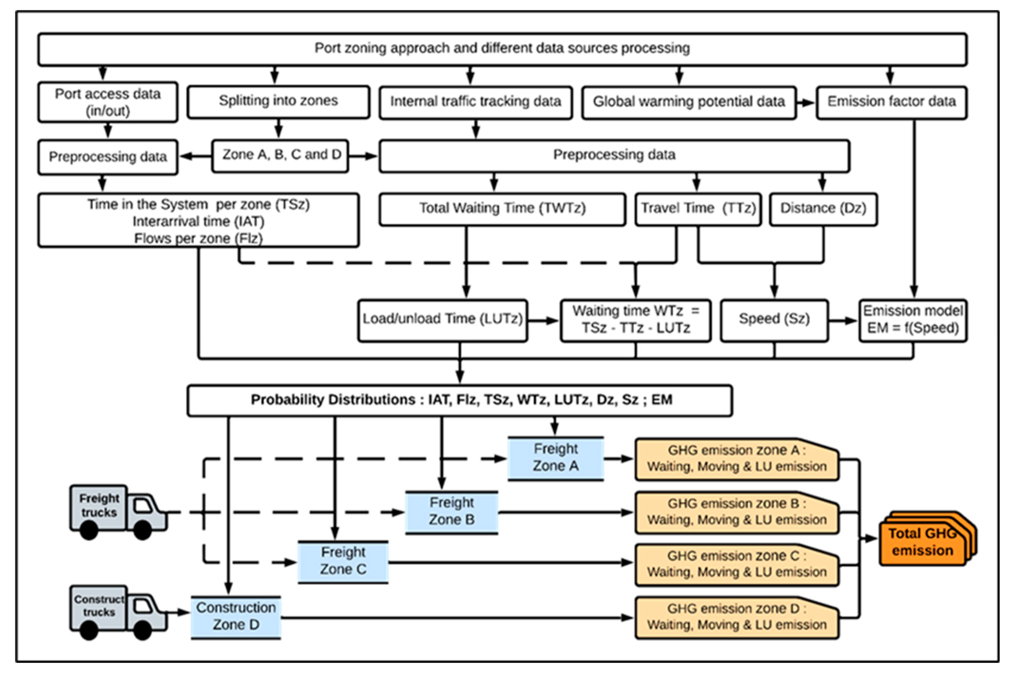
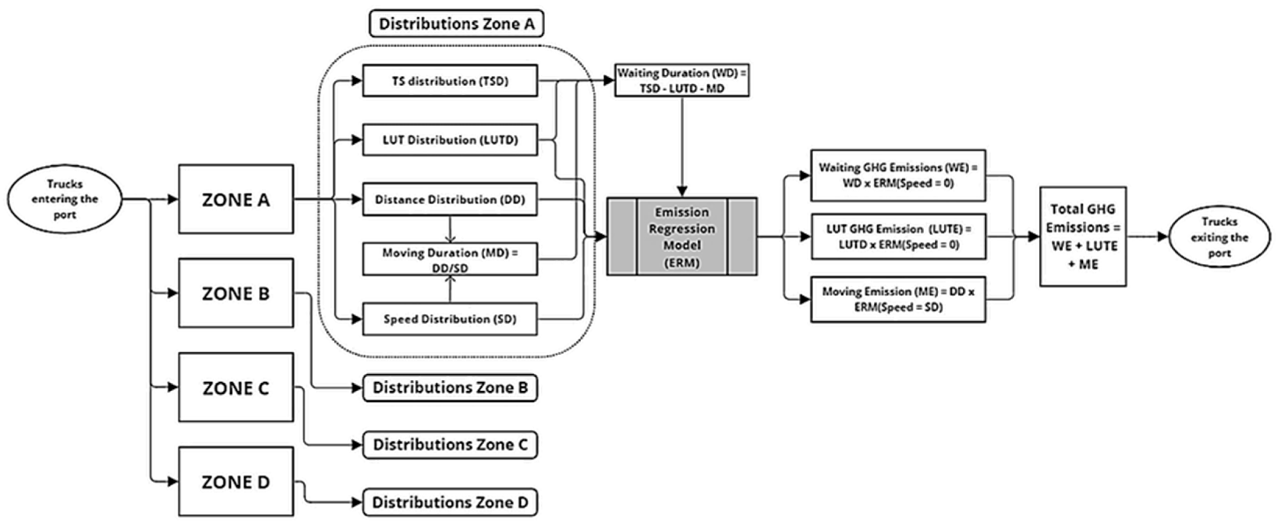
Our comprehensive methodology consists of several key components: the study area, data collection and processing, and the creation and implementation of both a GHG emissions model and a simulation model. The simulation model enables the assessment of emissions by replicating traffic activities within the port using a scenario analysis approach. Figure 1 provides a visual representation of the complete framework, which will be detailed in the following sub-sections.

3.1. Study Area

Situated on the St. Lawrence River, the Port of Trois-Rivières is a central hub within an extensive intermodal network that integrates rail, road, and sea transportation for national and international destinations. Established in 1882, the port plays a crucial role in regional, national, and international economic development across major industrial sectors. Strategically positioned halfway between the two main metropolitan areas of Quebec, Canada (i.e., Montreal and Quebec City), this port is highly sought after as a diversified transshipment center, handling a wide range of goods such as food, industrial, forestry, and consumer goods as well as other supplies. Each year, over 43,000 trucks, 10,000 railcars, and 250 ships access the port to load or unload cargo, with annual traffic consistently growing beyond 3.5 million metric tons [41]. The port comprises various terminals, which are categorized into zones based on the types of goods managed, including a general cargo terminal, grain terminal, and liquid and solid bulk terminal. To enhance the port’s overall capacity, a new terminal project is slated for construction over a two-year period, which is expected to result in a significant increase in traffic [41].

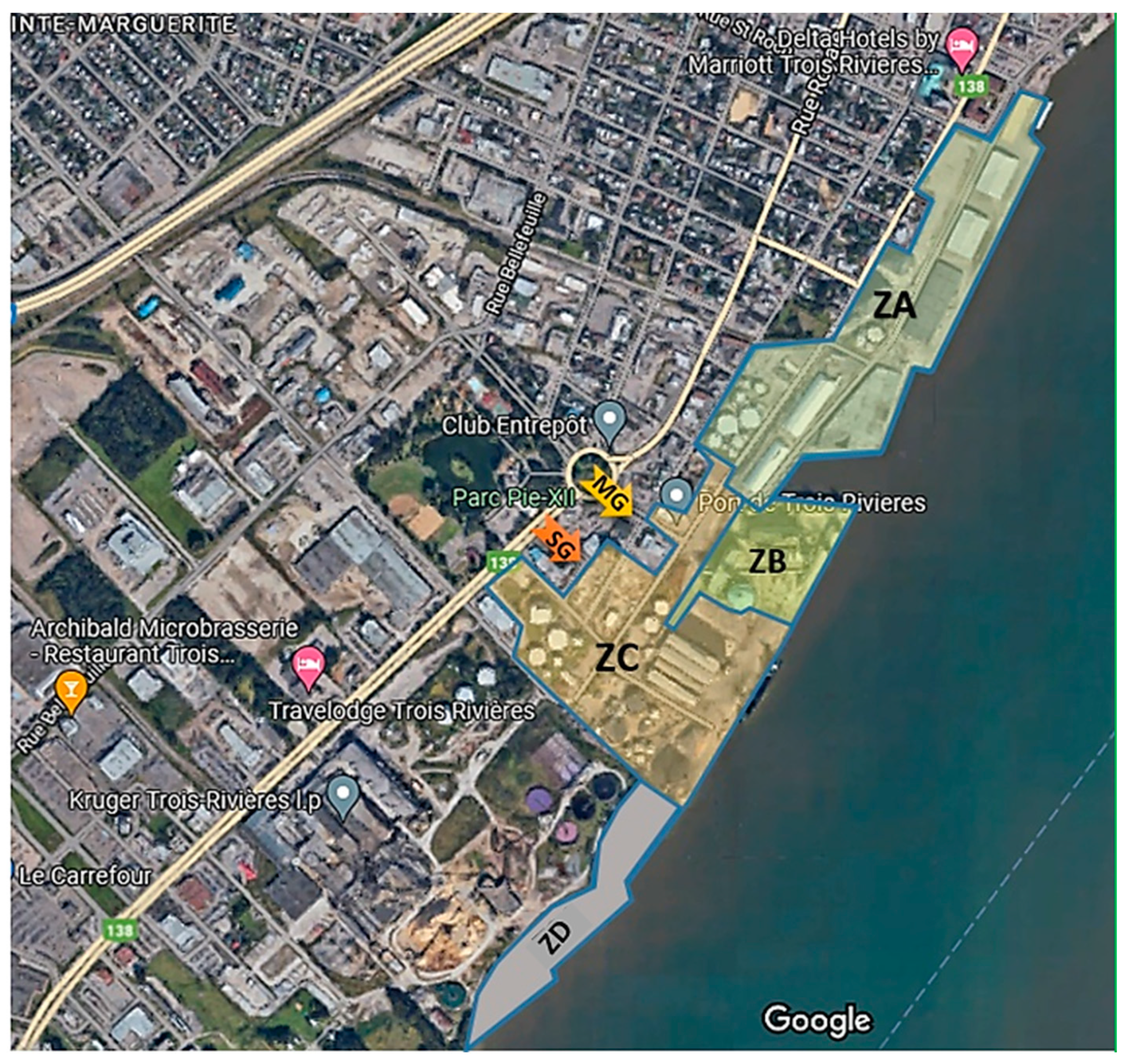
For the purpose of this study, the port was divided into distinct zones based on the types of goods handled in each area. These zones include Zone A, which is a general cargo terminal; Zone B, a grain terminal; Zone C, a liquid and solid bulk terminal; and Zone D, a new terminal project designated as Terminal 21. This classification allows for a more targeted analysis of the port’s operations and their respective emissions.

At present, there are two access gates for the port. The main access gate (MG) features three entries and one exit, while the secondary access gate (SG) has one entry and one exit. Figure 2 depicts the locations of the access gates and the respective zones.

3.2. Data Collection, Processing, and Analysis

The data employed for this research were derived from various sources, primarily the port information system. A differentiation is made between access data associated with the registration of trucks entering and exiting the port and data obtained from a detection system technology installed in different port zones to record internal traffic. Additionally, formal data on emission factors and GHG-related global warming potential were gathered from other sources, ensuring a comprehensive understanding of the port’s environmental impact.

3.2.1. Historical Access Data

An in-depth analysis of historical access data resulted in us selecting the years 2017–2019 as the foundational period for the study, specifically to avoid the distortions caused by the pandemic period. The chosen data were processed to eliminate recording errors or extreme values related to vehicles outside the scope of our research or exceptional operations not connected to the port’s routine activities. The historical data encompass the entry and exit times of each vehicle type (truck, car), access gates (MG, SG), and access mode (automatic, manual). A method was employed to categorize trucks by destination zone (A, B, C, and D), as outlined in Section 3.1, considering the geographical specificities that impact the time spent in the system, the distance traveled, and the speed of traffic within the port. The historical access data were utilized to determine the TS distributions by zone, the inter-arrival time, and the truck flow for each zone.

• Time in the System

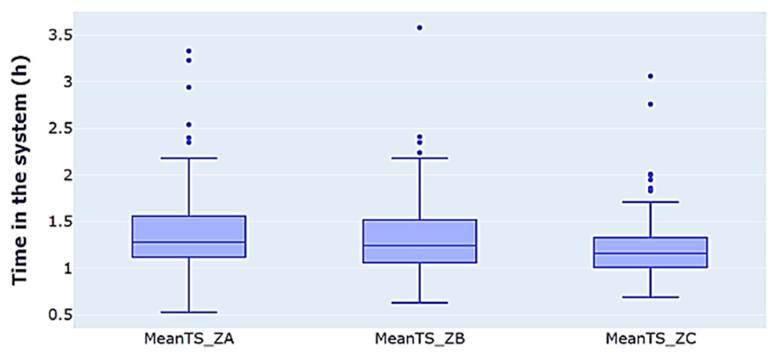
From the 2017–2019 access data, the TS is established. Weekly averages serve as observations to form probability distributions for each port zone. Statistical indicators of this distribution are depicted by box plots for each zone, as illustrated in Figure 3.

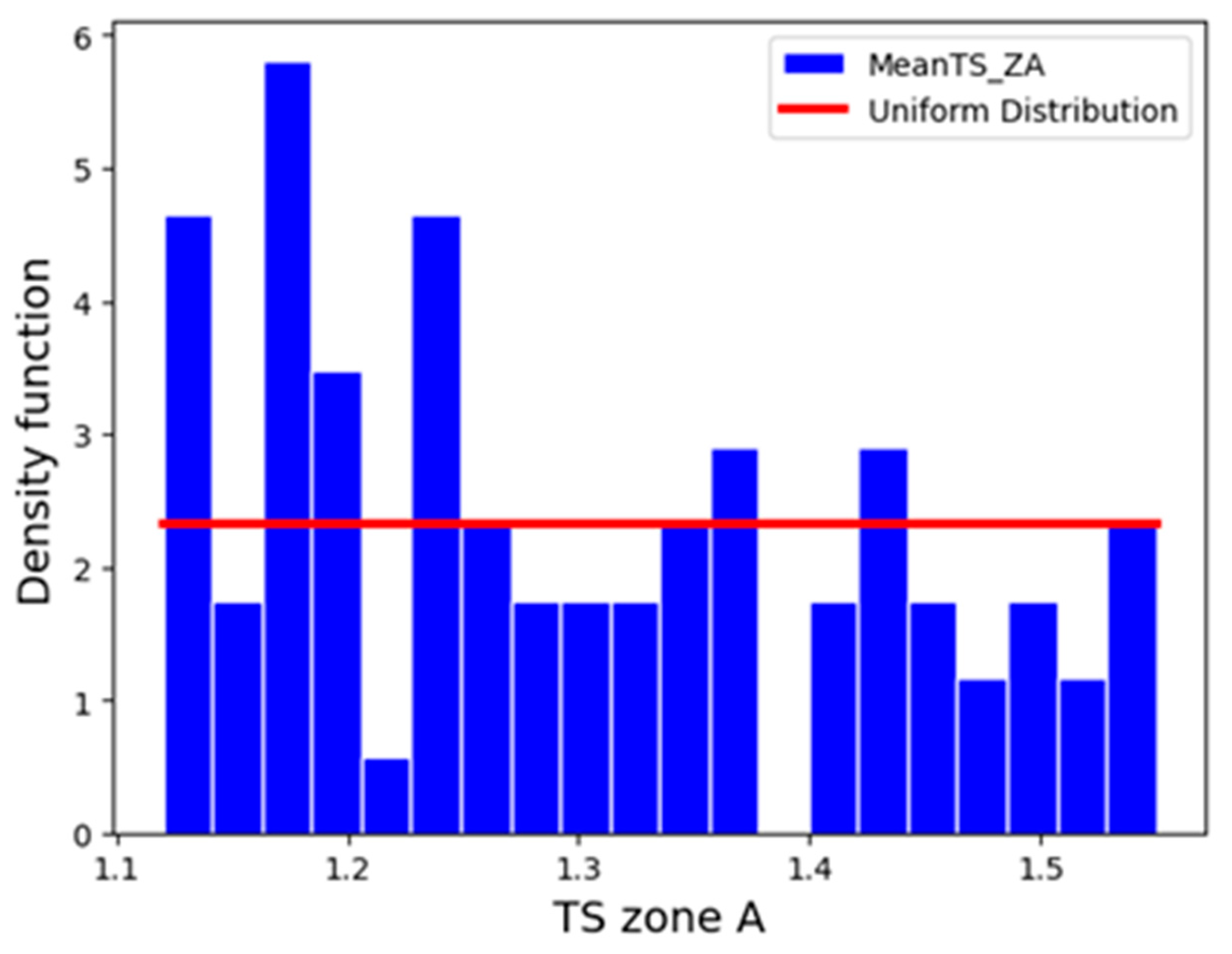
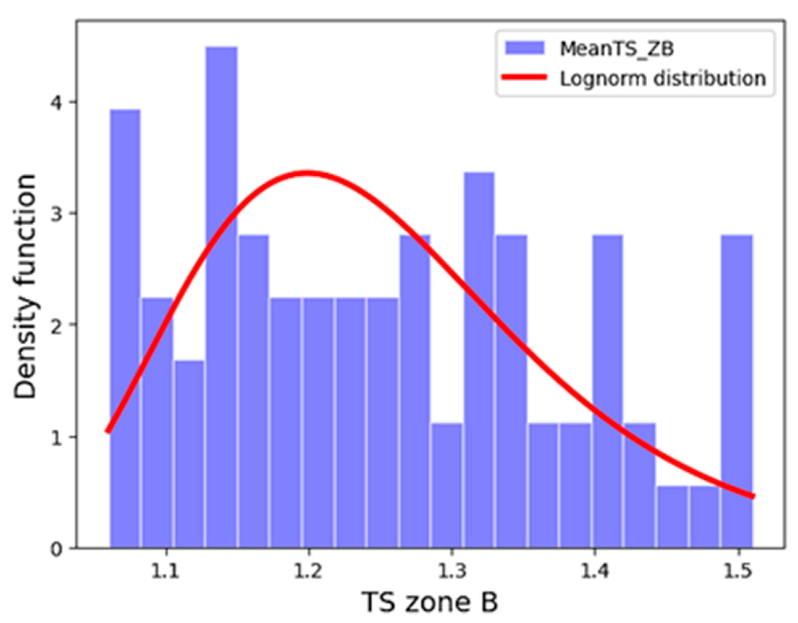
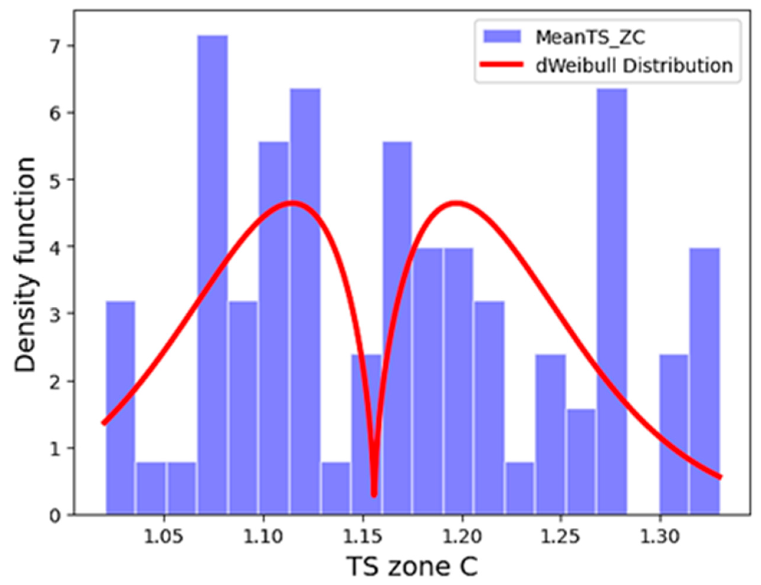
The TS parameter is a composite variable that includes travel time, waiting time, and loading/unloading time. Its variability can potentially affect the model’s convergence due to interference arising from the correlation between the TS and other time components within the system. To mitigate this dependency effect, we will limit the TS variability to fall between the first (Q1) and third (Q3) quartiles. This data adjustment enables the extraction of the most suitable probability distributions for the TS in each zone, as shown in Figure 4 for Zone A, Figure 5 for Zone B, and Figure 6 for Zone C. For Zone D, the TS is estimated to average 1 hour, comprising 20 min of loading/unloading time (LUT), based on data provided by the port authorities.

• Inter-Arrival Time and Truck Flow by Access Gate

The inter-arrival time (TIA) parameter is calculated based on the daily truck flow derived from the average number of trucks visiting the port per year, using the reference period of 2017–2019. After data cleaning, the daily number of freight trucks is found to be 118. However, for construction trucks, the port authority’s forecasts indicate an average of 145 trucks per day. As a result, using historical access data, the TS and TIA are ascertained. This facilitates the computation of the time spent in the system and the distribution of trucks—either freight (Zone A, B, and C) or construction (Zone D)—across access gates: 72% through MG and 28% via SG.

3.2.2. iNode Data Collection

Data are gathered from re-identification sensors (iNode), radar sensors, and connected truck technologies. The raw data supplied by the port information system are crucial due to the internal traffic patterns they encompass. Approximately 29 sensors are installed at various sites within the port areas to record internal truck traffic. The collected observations primarily concern Zones A and C, while estimates were made for parameters related to Zone B and the future Zone D, as detailed in the rest of the sub-section.

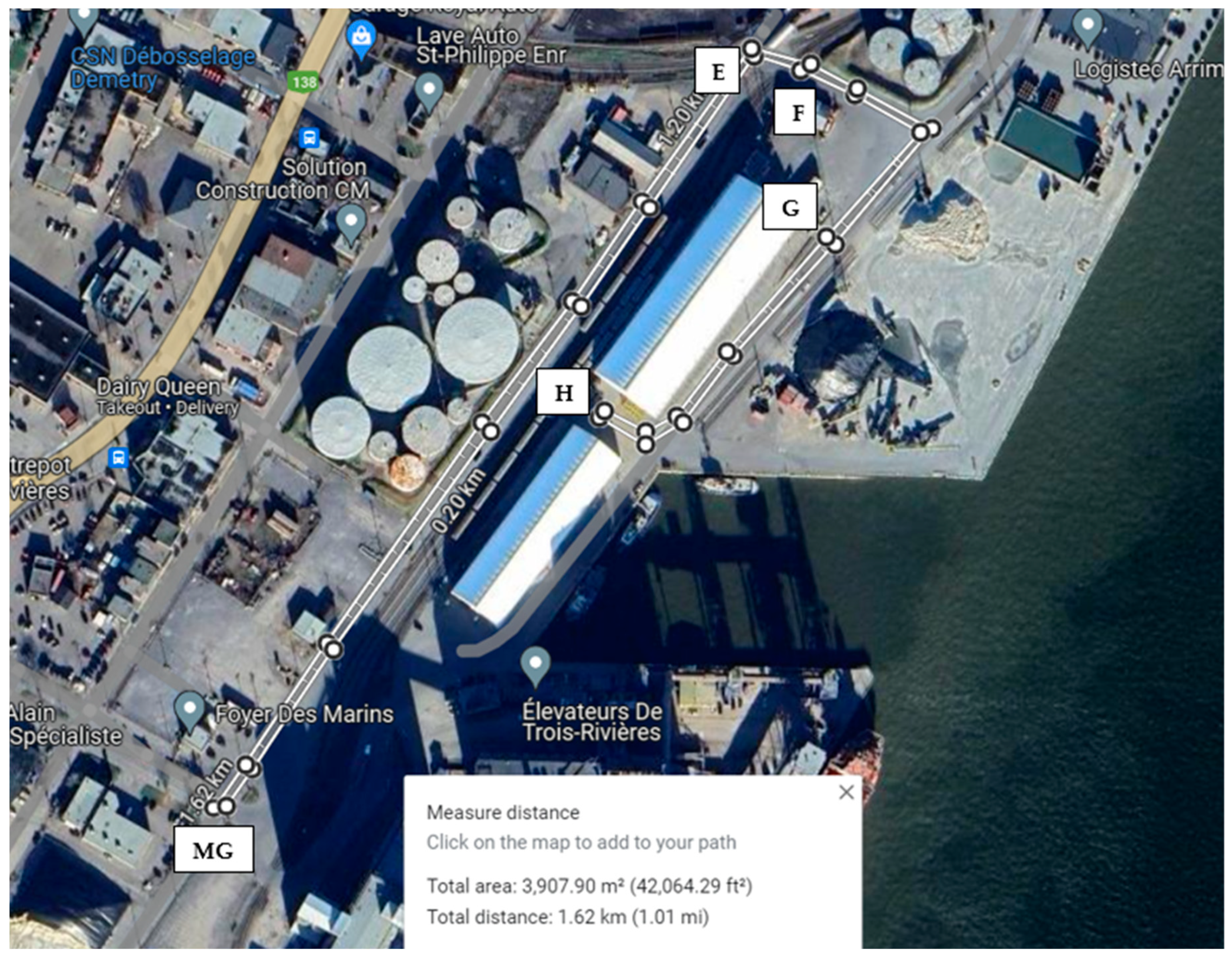
The data obtained consist of information regarding a sample of routes taken by monitored trucks (raw data of 3650 observations in total). Each route is represented as a sequence of nodes that specify the waiting time at each node and the travel time between every pair of nodes. An example of the raw data is provided in

Table 1. Original and processed data related to a single truck route observation.

	Route	Wait Times	Travel Times
Raw data	MG → E → F → G → H → G → F → E → MG	0:01:06 → 0:00:00 → 0:01:49 → 0:00:00 → 0:00:06 → 0:09:35 → 0:01:57 →0:00:08 → 0:00:00	0:02:09 →0:01:48 → 0:01:11 → 0:00:28 → 0:00:43 → 0:01:40 → 0:02:25 → 0:00:57
Computed data	1.62 km	Waiting Times = 0.25 h LUT = 0.16 h	0.189 h

, and a visual representation of one of the routes can be seen in Figure 7.

Advanced processing techniques were employed to extract key parameters that describe the truck traffic profile in various port areas from the raw data. In the first step of data processing, the following metrics were calculated for each route:

• Distance traveled;
• Average speed;
• Waiting time;
• Loading/unloading time (LUT);
• Travel time.

The parameters mentioned earlier are calculated by examining the nodes and arcs in each route, as demonstrated in the following computations:

• Travel time: the total time spent between traversed nodes is computed by summing the times, resulting in 0.189 h.
• Distance: the total distance between traversed nodes is computed by summing the distances, resulting in 1.62 km.
• Speed: the average speed is calculated by dividing the distance by the travel time, resulting in 8.57 km/h.
• Waiting times, including loading/unloading times: the waiting times are determined by adding up the times recorded at each visited node, resulting in 0.25 h.
• Loading/unloading time: the highest waiting time is defined to be the loading/unloading time, resulting in 0.16 h.
• Waiting times other than loading/unloading time: the waiting time excluding loading/unloading time is calculated by subtracting the loading/unloading time from the waiting times, resulting in 0.09 h.
• Time in the system: the total time spent in the system, including loading/unloading time, waiting time, and travel time is calculated by summing these times, resulting in 0.439 h.

The initial processing of the data reveals the presence of outliers for all parameters; these are presented in

Table 2. Descriptive statistics of raw data after the first processing step, including mean, standard deviation, minimum, maximum, and quartile values for various parameters.

Stat.	Distance (km)	Time (minutes)
		Load/Unload	Travelling	Waiting
count	3650	3650	3650	3650
mean	2.0	34.7	12.4	57.5
std	2.2	30.8	31.1	42.7
min	0.0	0.0	0.0	0.0
25%	0.7	13.2	1.1	28.3
50%	1.5	27.9	2.2	46.3
75%	2.5	43.5	10.1	74.7
max	49.7	213.6	678.6	340.2

.

The broad range of parameter values observed calls for a detailed treatment to remove any outliers that may not accurately represent regular freight activity. For instance, speeds close to zero indicate micro-stopovers along the route, while excessively high speeds may result from erroneous truck detection. To address these anomalies, we employed a processing approach that leverages statistical rules and other techniques to identify relevant observations and their associated probability distributions for each parameter. The steps taken to achieve this are described below.

• Loading/Unloading Time

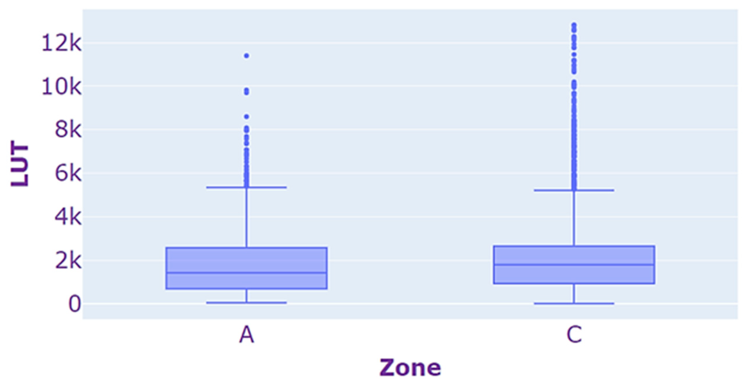
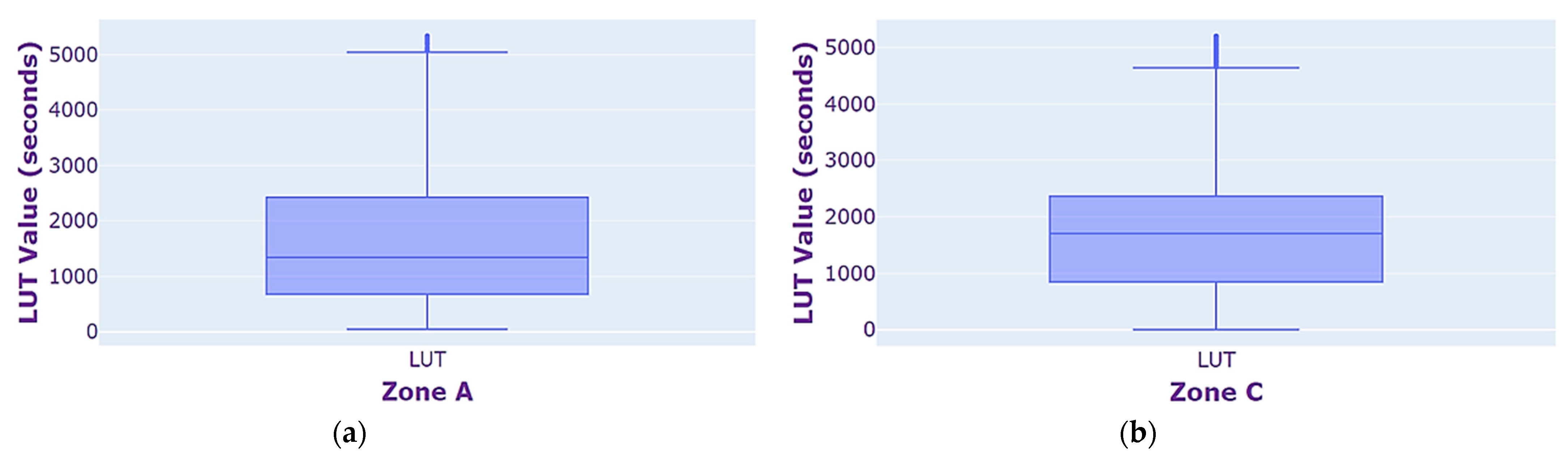
The LUT parameter, as mentioned earlier, is estimated as the longest waiting time registered in a node along a given route. However, this parameter may present outliers, particularly when it overlaps with waiting times not related to loading or unloading. These outliers are illustrated in the box plot shown in Figure 8.

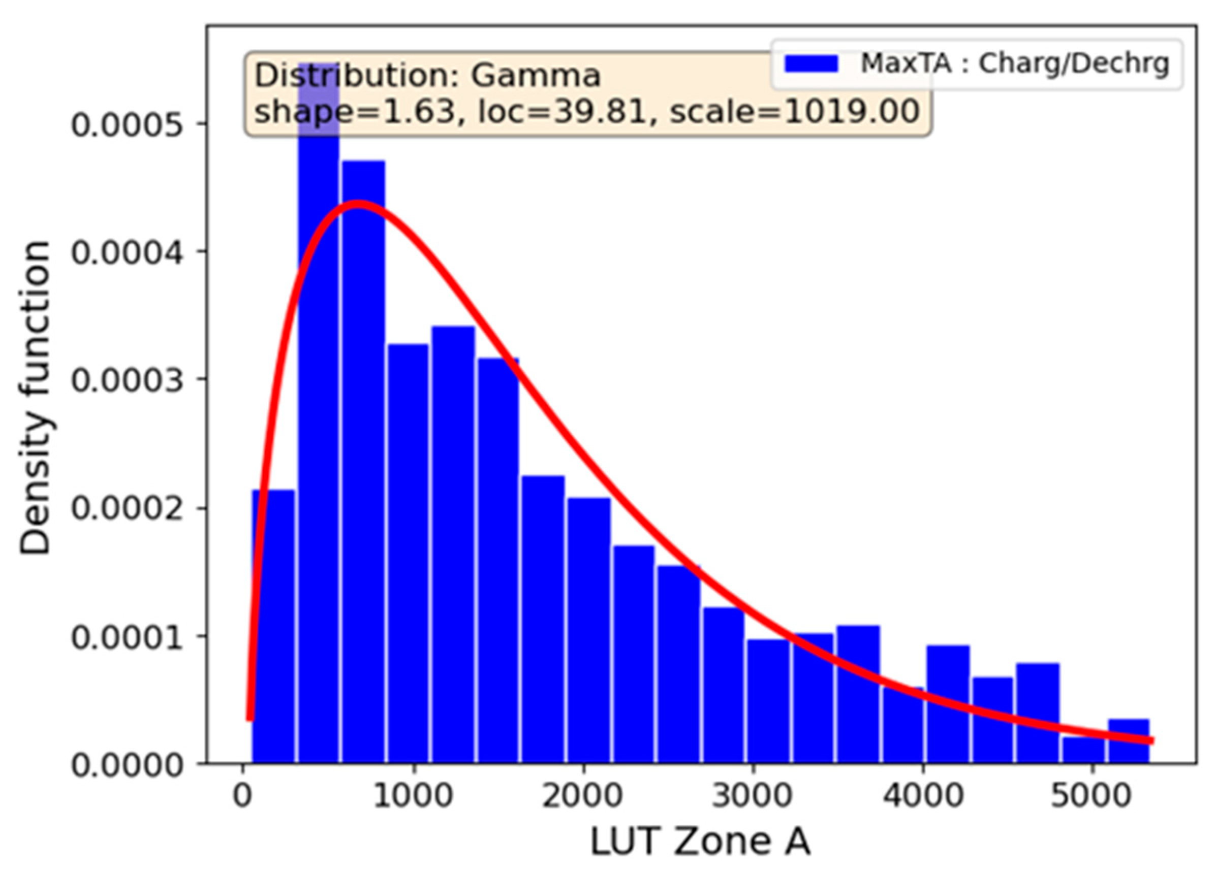
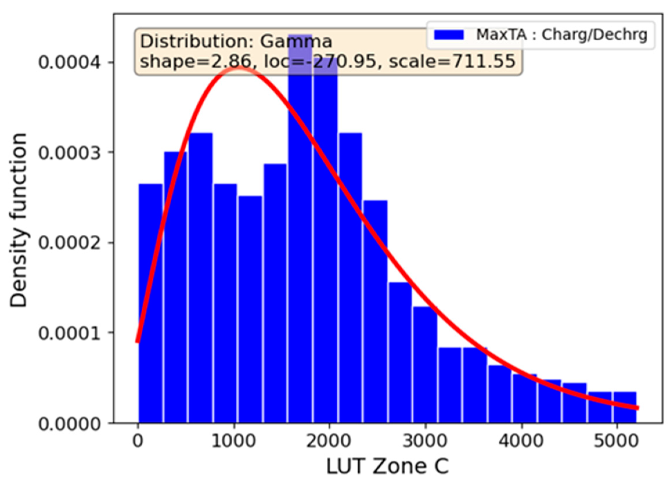
To remove any outliers and address the distortion of the LUT parameter, we made adjustments to limit the LUT value between Q1-1.5IQR and Q3 + 1.5IQR. This approach adheres to statistical rules that remove aberrant values, where Q1 and Q3 are the first and third quartiles, respectively, and IQR is the interquartile range (Q3–Q1). Figure 9 depicts the distribution of the LUT observations after this adjustment.

The adjusted observations were used to generate the required probability distributions of the LUT parameter for Zones A and C, as illustrated in the frequency distributions and distribution curves presented in Figure 10 and Figure 11. The gamma distribution was found to be the most suitable for modeling the LUT parameter in both zones. The average LUT for Zones A and C was validated by comparing it to an empirical study conducted previously in the port [42].

For the LUT parameter in Zone B, the parameters of a triangular distribution (min, mean, and max) were also derived from the results of the aforementionned empirical study [42]. As for Zone D, the LUT parameters were obtained from the port authorities, who provided data based on past experience from a previous terminal construction. The LUT in Zone D was observed to range between 15 and 25 min, with an average of 20 min. These parameters were used to construct a triangular distribution for the LUT parameter in Zone D.

• Speed

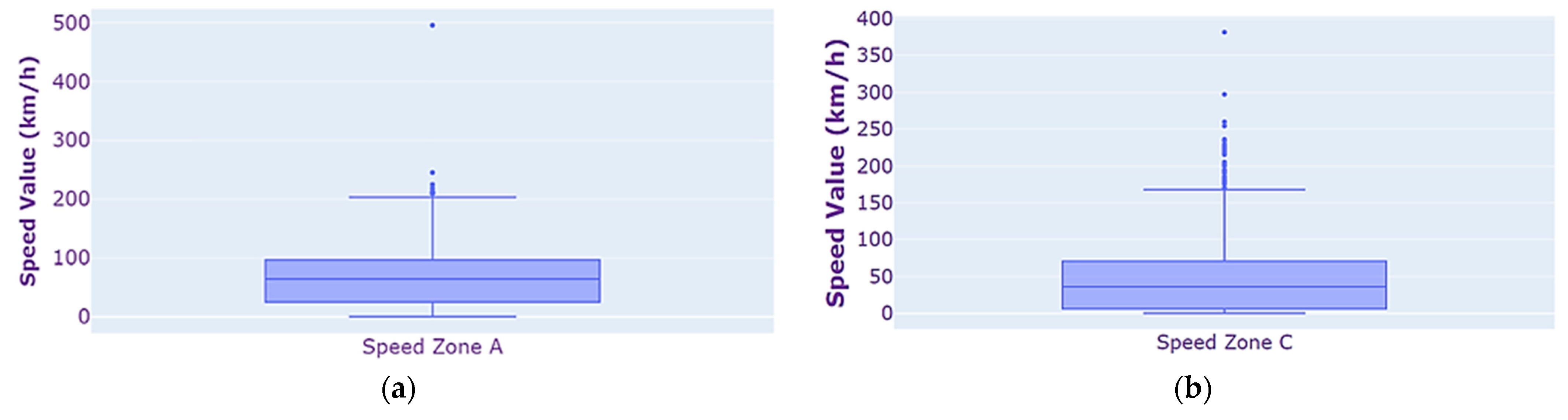
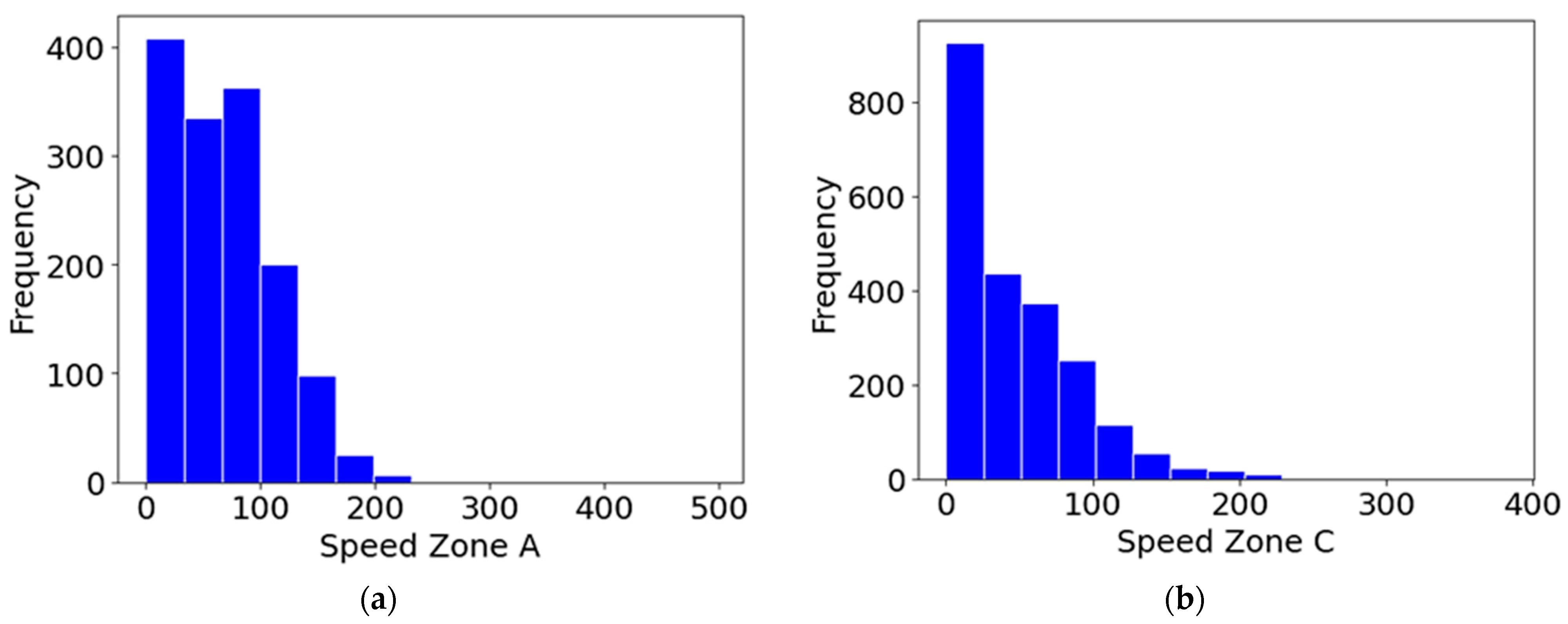
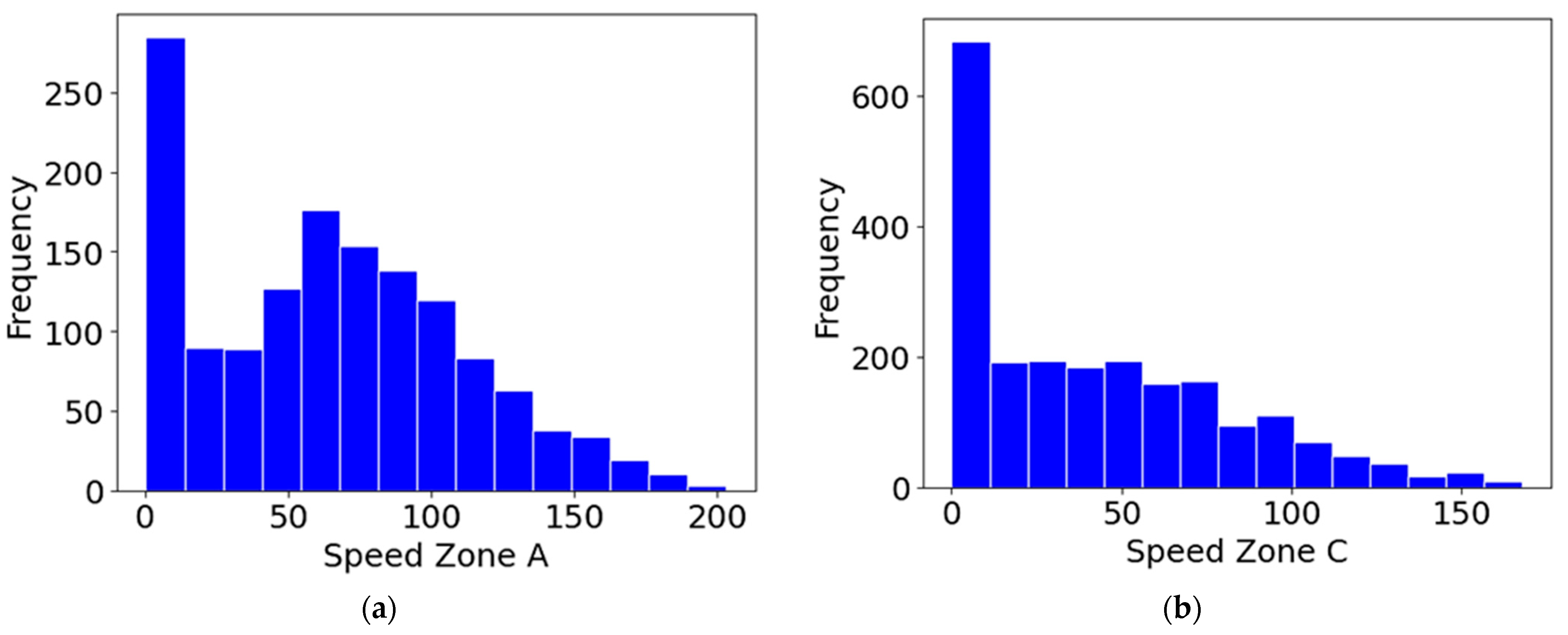
As depicted in Figure 12 and Figure 13, the captured speeds have outliers that may represent micro-stopovers between nodes, leading to small speeds or inflated speeds, likely due to position adjustments of the tracking sensors.

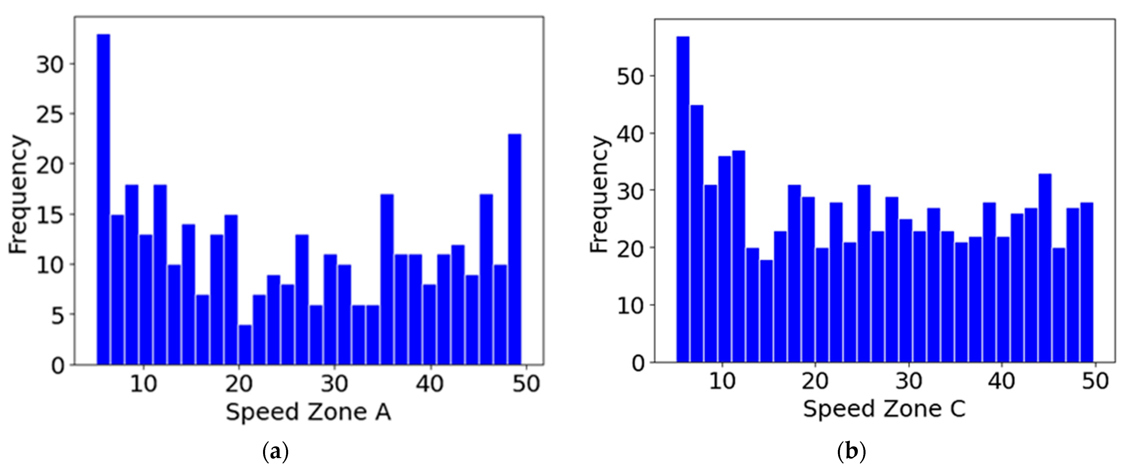
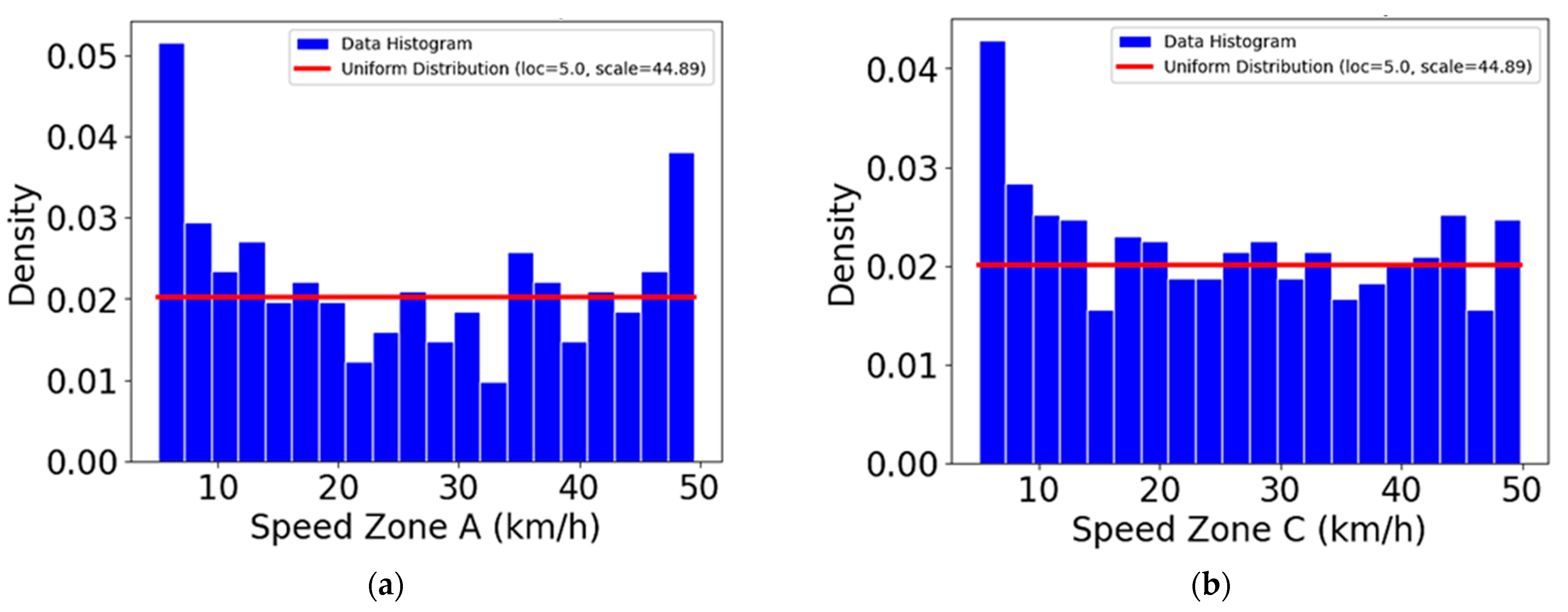
To address the outliers observed in the captured speeds, the first adjustment step was to follow the same statistical rule used for the LUT parameter. The output of this adjustment is shown in the histograms presented in Figure 14. However, to avoid speeds that are too low or exceed the third quartile, it was determined that the speed should be adjusted to fall between 5 km/h (minimum truck speed similar to walking speed) and 50 km/h (typical maximum urban traffic speed even if the internal rules of the port limit the speed to 30 km/h). The frequency and fitting distribution of the adjusted speeds for Zones A and C are shown in Figure 15 and Figure 16, respectively. For Zone B, the adopted speed is the average of the speeds observed in Zones A and C, while for Zone D, the speed is set to be the same as that of Zone A, given their similar average distances.

• Distance

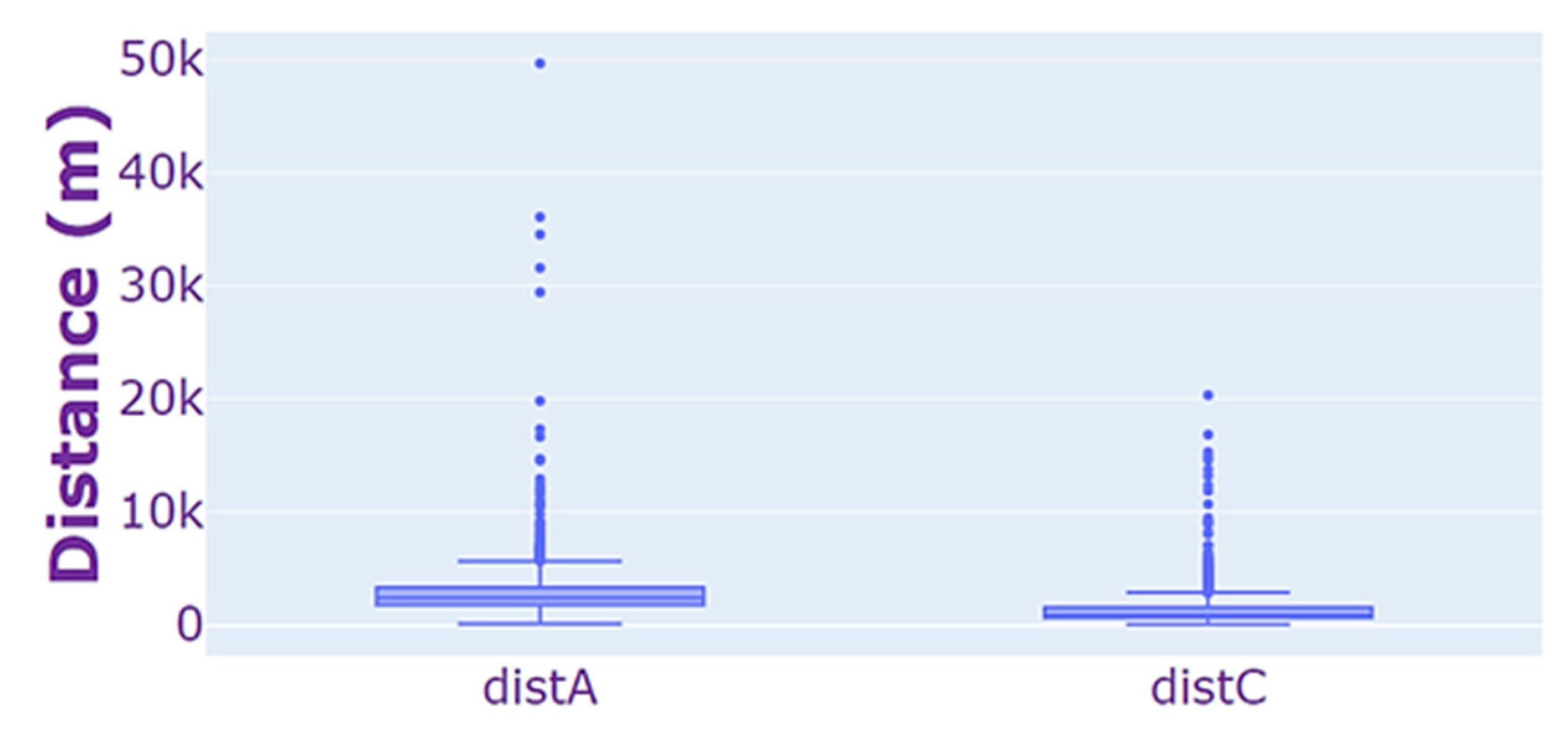
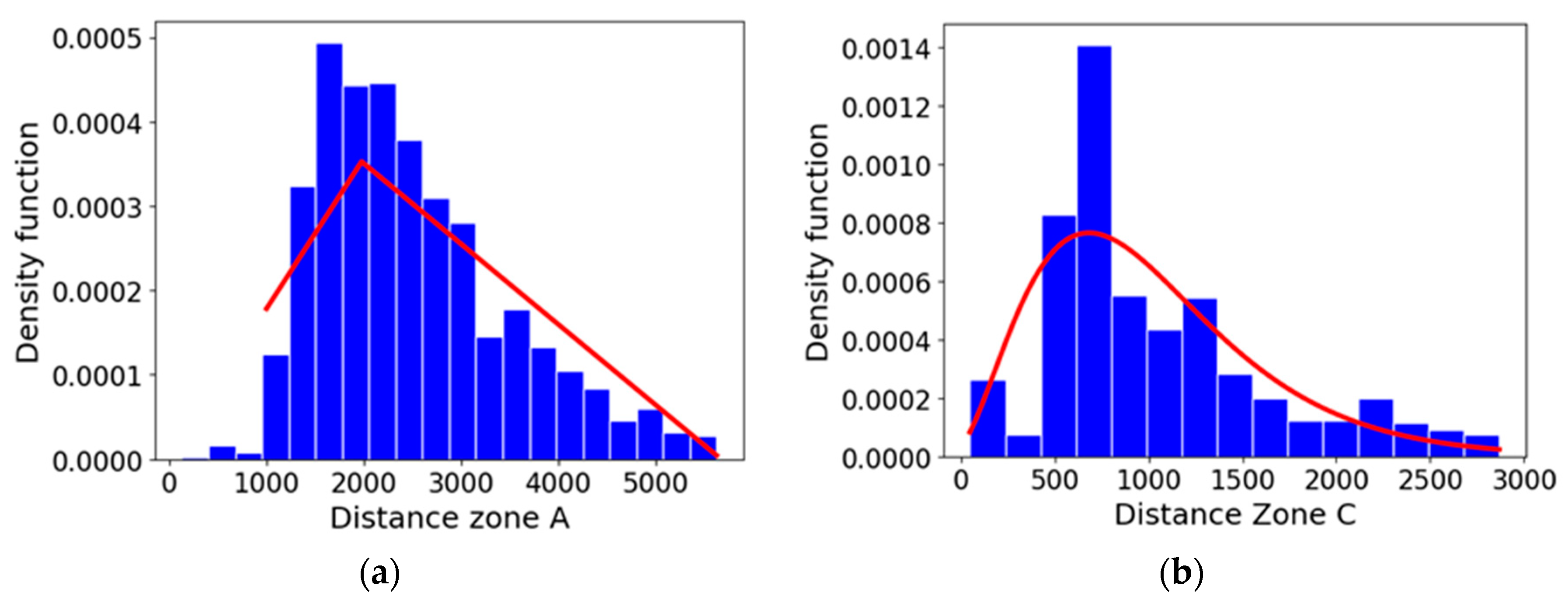
The distance values of the truck routes also show some aberrations, as can be seen in Figure 17, which may be due to the internal operational activities of the port. To address this issue, the statistical rule of interquartile adjustment was applied, which effectively solved the problem. Two fitting distance distribution probabilities were then performed for Zones A and C, as shown in Figure 18.

To generate the triangular distribution probability of the distance parameter, the value of Point c (mode value) was determined for each zone according to the formula:$\frac{\max \left(d\right)-2{(\max \left(d\right)-median\left(d\right))}^2}{(\max \left(d\right)-min\left(d\right))}$, where d is the distance. Nevertheless, for Zones B and D, their respective distance distributions were approximated using measurements from Google Maps for the specific route that must be followed by trucks visiting these zones, with an allowance for a 20% deviation in either direction.

Six probability distributions were employed to characterize the historical data, as summarised in

Table 3. Probability distributions adopted for modeling various parameters.

Probability Distributions
Zone	TS	LUT	Distance	Speed
A	Uniform	Gamma	Triangular	Uniform
B	Lognl	Triangular	Normal	Uniform
C	Weibull	Gamma	Gamma	Uniform
D	Uniform	Triangular	Normal	Uniform

; they estimate the likelihood of observing parameter values for travel time, distance, LUT, and speed in different zones of the port area.

3.3. GHG Model Based on the Speed

The GHG emissions model aims to assess the emissions produced by trucks within the port area. The model considers the two main truck behaviors within the port: waiting and traveling. Waiting includes both loading/unloading and queueing. The model characterizes the state of the truck and calculates the corresponding emissions for each state using speed, distance traveled, and waiting time. To calculate travel and waiting emissions, we established a correlation between speed and GHG emissions for each of the three primary gases that contribute to global warming: CO₂, CH₄, and N₂O. This approach draws inspiration from a method used by the San Pedro Bay Ports of Long Beach and Los Angeles [5]. Other emissions listed in [5] are associated with different air pollutant emissions but are not GHGs and are thus excluded from our study.

Table 4. GHG emissions based on the speed of the truck (adapted from [5]).

Speed (mph)	CO2	CH4	N2O	Units
0 (Idle)	6082	0.6750	0.8982	g/h
5	3691	0.4985	0.5912	g/mi
10	3176	0.3279	0.5082	g/mi
15	2609	0.1929	0.4168	g/mi
20	2275	0.1349	0.3633	g/mi
25	2051	0.1027	0.3273	g/mi
30	1880	0.0821	0.3000	g/mi
35	1748	0.0679	0.2788	g/mi
40	1649	0.0576	0.2630	g/mi
45	1580	0.0498	0.2519	g/mi
50	1539	0.0439	0.2453	g/mi
55	1525	0.0392	0.2429	g/mi
60	1549	0.0390	0.2467	g/mi
65	1607	0.0391	0.2558	g/mi
70	1607	0.0391	0.2558	g/mi

shows the speed intervals and the corresponding emissions for trucks.

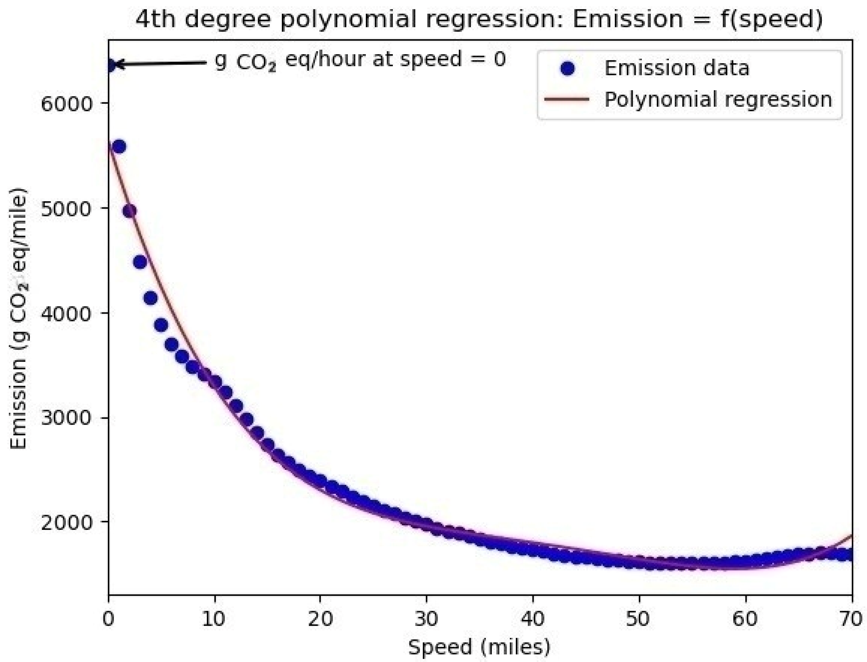
From Table 4, we aggregated GHG emissions into gram CO₂ eq/mile. To convert the emission model described in Table 4 into a model in CO₂ equivalent units, we used the values of global warming potential for each type of GHG, as determined by the IPCC [43]: CO₂, CH₄, and N₂O emissions were multiplied by 1, 25, and 298 respectively. Then, several regression models were used to interpolate the discrete interval points in Table 4 for different values of speed for a truck t from s_t = (0, …70) miles per hour to create a smooth curve that shows a continuous correlation between speed and emissions. A fourth-degree polynomial model was selected and fitted, with a coefficient of determination of 0.985, to establish the correlation between speed and CO₂ equivalent emissions as demonstrated in

$$F\left(s_t\right)={0.0012s_t}^4-{0.2071s_t}^3+{13.251s_t}^2-387.18s_t+6259.1$$

(1)

where

$F\left(s_t\right)$ denotes the GHG emissions per hour (s_t = 0) or per mile (s_t > 0) according to the speed of the truck.

The fitted model is depicted in Figure 19, and it applies from zero speed, when the truck is in a waiting state, to 70 miles per hour when the truck is moving. For the waiting state, the emission model is applied to each waiting hour; meanwhile, in the traveling case, the model applies to each mile driven.

3.4. The Global Emission Model

The global emissions produced by truck traffic in the port are computed by

$${GHG}_{GE}={\sum }_z{\sum }_t{E}_{{tr}_{t,z}}+{\sum }_z{\sum }_t{E}_{w_{t,z}} ;z=Zone A, B, C And D;t=truck \mathrm{1,2}..n$$

(2)

where

${GHG}_{GE}$ denotes the GHG global emissions for the trucks visiting the port.

$E_{{tr}_{t,z}}$ denotes the GHG emissions of the truck t in travelling state visiting the zone z.

$E_{w_{t,z}}$ denotes the GHG emissions of the truck t in waiting state visiting the zone z.

The travelling emission is defined as the product of the distance traveled in miles and the travelling speed emission determined according to Equation (1); it is expressed as

$$E_{{tr}_{t,z}}=F\left(s_t\right)D_{t,z} , s_t>0$$

(3)

where

$D_{t,z}$ denotes the distance travelled in miles by the truck t in the zone z.

$$E_{w_{t,z}}=F\left(s_t\right){WT}_{t,z} , s_t = 0$$

(4)

$${WT}_{t,z }={LUT}_{t,z}+{OWT}_{t,z}$$

(5)

where

${WT}_{t,z}$ denotes the waiting time recorded in hours by the truck t in the zone z.

${LUT}_{t,z}$ denotes the loading/unloading time recorded by the truck t in the zone z.

$${OWT}_{t,z}={TS}_{t,z}-{LUT}_{t,z}-{TT}_{t,z}$$

(6)

where

${OWT}_{t,z}$ denotes the other waiting time recorded by the truck t in the zone z.

${TS}_{t,z}$ denotes the TS recorded by the truck t in the zone z.

$${TT}_{t,z}=D_{t,z}/s_t$$

(7)

where

${TT}_{t,z}$ denotes the travel time recorded in hours by the truck t in the zone z.

To validate the emissions model adopted, its predictive results were compared with those reported in the literature reported for similar contexts. Roso [44] reported that trucks emit 6000 g/h of CO₂ while idling. Quiros et al. [45] reported an emission of 3055 g/km CO₂ eq for conventional diesel trucks from the year 2007 in an urban context with a speed of 7.8 mph. Abou-Senna and Radwan [46] revealed that there is a significant potential for reducing emission levels at specific travel speeds, particularly between 55 and 60 mph. A study conducted by Barth and Boriboonsomsin [47] revealed a rapid, non-linear increase in pollutant emissions and fuel consumption when vehicle speeds drop below 30 mph. Li et al. [48] reported CO₂ levels close to 1000 g/km at a speed of 60 km/h (37.3 mph) for heavy-duty diesel trucks in Beijing. These results show that the adopted GHG emissions model provides a good outcome and is consistent with some research work on the port context.

Regarding the epistemological position of the developed model, it appears to lean more toward the mesoscopic approach. As documented in the literature, meso-models allow for modeling the carbon footprint and its impacts by combining the advantages of macroscopic and microscopic approaches. This could be considered an intermediate scale between a global view and an extremely detailed view. Compared to microscopic models that focus on individual behaviors and specific entities in real time, meso-models are less demanding in terms of computational resources and rely on average data to assess the carbon footprint (as is the case for this work), since the input of the developed model is the average speed for a fleet of port trucks. However, the accuracy of meso-models depends on the quality of the input data.

3.5. Simulation Model

A simulation model was developed using Simio version 15 to evaluate the emissions generated by trucks within the port. This model aimed to replicate the behavior of trucks using stochastic parameters derived from historical data, and it incorporated the global emission model to calculate GHG emissions. The Simio library was utilized to establish the different flows, entrance/exit gates, and zones (A, B, C, and the new terminal D) within the port. Stochastic simulation parameters were implemented within various objects and processes to model truck behavior.

The simulation system comprises two flow sources, each dedicated to a specific vehicle type: freight trucks and construction trucks. Based on the historical data, it allocates each vehicle to a specific destination zone and follows a stochastic time schedule tailored to the assigned area. Then, the simulation assigns stochastic parameters to each truck to determine their loading/unloading times, speed, and distance. Upon completion of the time schedule for the zone, the truck leaves the port through a specific exit gate.

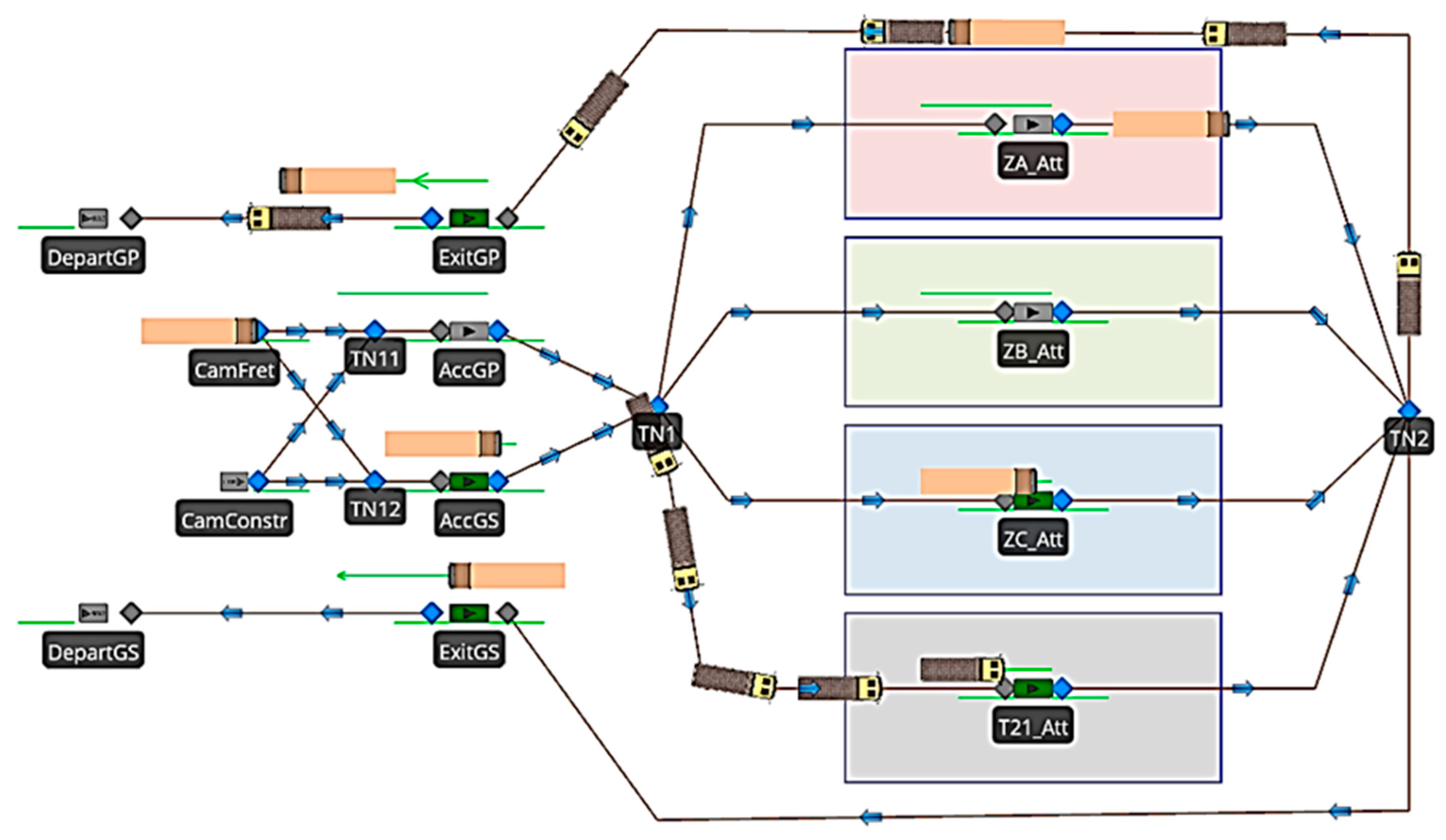
To simulate the truck flow for a day, the simulation model is configured accordingly. The inter-arrival time of trucks is defined as a function of the simulated period divided by the number of trucks expected to attend the port during that time. To achieve a stationary state, the simulation model operates for a duration of 30 days. This extended running time is necessary to plan and conduct simulation experiments effectively. Furthermore, the simulation model underwent validation through an adequate number of replications, ensuring convergence towards the mean of its stochastic parameters. This specific count of replications was chosen to generate results for subsequent analyses. The design of the simulation model is depicted in Figure 20.

Trucks were assigned to specific zones based on probabilities that reflect historical traffic flows. These assignments consider several parameters, including distance, speed, the duration of loading/unloading, and the overall time spent within the system. To calculate travel time, the model divides the distance by the speed. Furthermore, it determines other waiting times by subtracting the sum of travel time and loading/unloading durations from the total time in the system. The emission calculations utilize a regression model that distinguishes between idle (accounting for both loading/unloading durations and other waiting times) and travel states. For the idle state, the regression emission model assigns emissions equivalent to zero speed, whereas for the traveling state, it assigns emissions corresponding to the actual moving speed. These calculations are based on the duration of idle states and the distance covered during the travel state. The aggregate emission value merges emissions from idling (including both loading/unloading and other wait times) and traveling. After completing their activities, trucks leave the port, and their emissions are added to the overall emissions count. Additionally, Figure 21 demonstrates the integration of the emission model within the simulation framework, providing a visual representation of how emissions are computed and attributed throughout the simulation process.

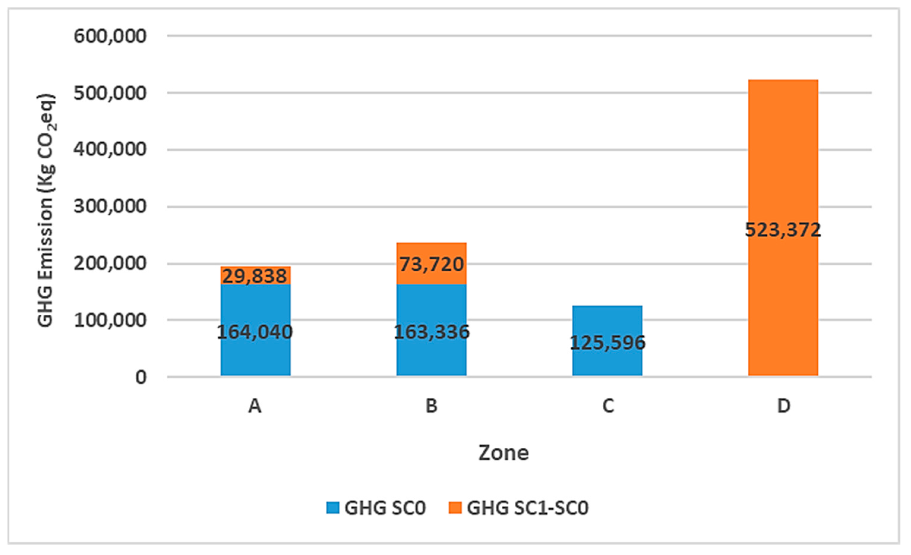
3.6. Scenario Design

The evaluation scenarios for the simulation model include a baseline scenario as a reference point and exploration scenarios for assessing emissions under various prospective contexts. These scenarios are designed to account for the anticipated increase in the number of trucks visiting the port and the impact of trucks during the construction period. The data provided by the port authority indicate that the number of freight trucks is expected to increase by approximately 23% over this period, while construction trucks are forecasted to average 145 trucks per day.

4. Evaluation Findings and Related Discussion

After validating all the implemented stochastic parameters, the simulation model was ready to present the results of the emissions evaluation for heavy-duty trucking within the port. In addition to the baseline scenario, the simulation model was also used to predict GHG emissions during the construction period of the new terminal. After conducting the prediction scenario, the results were analyzed and interpreted to gain insights into the impact of the construction period on GHG emissions in the port.

4.1. Baseline Scenario

The preliminary results of the simulation model, which ran for 365 days, reveal that GHG emissions from trucks vary depending on the zone within the port. Additionally, the emission structure within each zone differs based on the truck’s behavior states of moving, loading/unloading (L/U), and waiting.

Table 5. Overall annual result by zone.

Zone	Trucks Number	Distance (km)	Time (h)				GHG Emission (kg CO2eq)
			TS	LUT	Travelling	Waiting	L/U	Travelling	Waiting	Total	%
A	13,714	31,151	18,314	6286	1728	10,301	39,889	58,778	65,373	164,040	36.2
B	15,679	25,186	19,673	2823	1380	15,470	17,916	47,249	98,172	163,336	36.1
C	13,893	15,114	16,184	6918	810	8456	43,901	28,033	53,662	125,596	27.7
Total	43,286	71,451	54,171	16,027	3918	34,227	101,707	134,059	217,207	452,973	100

summarizes the results obtained for an annual activity of 43,286 freight trucks in the different zones of the port. The total annual GHG emission amounts to 453 tons, distributed as follows: Zone A (36.2%), Zone B (36.1%), and Zone C (27.7%).

On average, a truck in Zone A emits 12 kg of CO2eq, distributed as follows: travelling (36%: 4.3 kg of CO2eq), L/U (24%: 2.9 kg of CO2eq), and waiting (40%: 4.8 kg of CO2eq). Waiting is the most GHG-emitting behavior for all zones, accounting for 40%, 60%, and 42% of emissions for Zones A, B, and C, respectively.

Table 6. Summary of annual results for each zone, including the number of trucks, distances, times in the system, and emissions.

Zone	Trucks Number	Distance (km)	Time (h)				GHG Emission (kg CO2eq)
			TS	LUT	Travelling	Waiting	L/U	Travelling	Waiting	Total	%
A	16,138	37,260	21,545	7402	2080	12,066	46,970	70,339	76,568	193,878	18.0
B	22,722	36,576	28,540	4085	2021	22,433	25,924	68,771	142,361	237,056	22.0
C	13,857	15,077	16,148	6899	819	8429	43,781	28,093	53,493	125,367	11.6
D	53,688	119,246	53,678	17,913	6619	29,148	113,677	224,724	184,971	523,372	48.5
Total	106,405	208,159	119,910	36,299	11,539	72,076	230,352	391,928	457,394	1,079,674	100

and Figure 22 provide further details on the distance and time spent in the system.

Figure 23 depicts the average time and emissions per truck for each zone within the port.

4.2. Emissions Prediction for the Construction Period

The port authorities are anticipating a significant increase in the number of trucks visiting the port during the construction phase, primarily due to the presence of construction trucks at the new terminal (Zone D). Consequently, the simulation model parameters for flows and inter-arrival times will change. During this period, the global GHG emission is projected to double to 3 tons per day and will be distributed among Zones A (18%), B (22%), C (11.6%), and D (48.5%). Table 6, along with Figure 24, illustrate the numbers of trucks, distances traveled, and the details of times in the system and emissions for this period. These visual aids provide valuable insights into the anticipated impact of increased truck traffic on emissions and operational efficiency within the port system.

The total GHG emissions during the construction period are estimated to be 1079 tons annually, which represents a significant increase of approximately 138% compared to annual emissions under the baseline scenario. The increase in emissions is primarily due to the rise in the number of trucks using the port in Zones A (2440 trucks annually) and B (7250 trucks annually) and the trucks involved in the construction of the new terminal (an average of 145 trucks per day). This increase in truck traffic will result in a significant impact on GHG emissions within the port system.

Figure 25 illustrates the difference in the additional GHG emissions generated annually in the predicted scenario (SC1) compared to the baseline scenario (SC0) considering the incremental number of trucks visiting Zones A, B, and D.

Figure 26 shows the average GHG emissions and time per truck for each zone within the port.

4.3. Discussion

The outcomes derived from the simulation model underscore the distribution of GHG emissions across different zones and truck conditions, providing clear guidance for targeting and achieving GHG reduction goals. The findings reveal that a substantial portion of GHG emissions stems from waiting times within the port, making it the primary contributor. Consequently, priority efforts should concentrate on minimizing this factor. Chen et al. [49] assert that reducing emissions in ports hinges on diminishing waiting times, achievable through optimizing truck arrival coordination and upgrading port equipment.

Do et al. [50] suggest that emissions from truck waiting times can be significantly decreased by restricting the entry times for each truck. Among the most effective strategies for optimizing truck arrival scheduling is the adoption of a truck appointment system (TAS) in the USA or a vehicle booking system (VBS) elsewhere [51]. The TAS standardizes truck arrival rates, markedly reducing waiting times and subsequently curbing CO₂ emissions from heavy-duty vehicles at port terminals [23,52]. Morais and Lord [53] conducted a study for the Canadian government, affirming the successful implementation of a TAS at the Port of Vancouver and offering recommendations for its effective adoption elsewhere.

Additional measures to decrease waiting times encompass documenting the fuel consumption profiles (such as age, engine speed, etc.) of the port’s truck fleets to pinpoint inefficiencies, implementing GPS trackers to optimize routes and minimize stops, and instituting compulsory, recurring training programs for truck drivers. This program aims to increase awareness of access and traffic issues, discouraging engine idling, and promoting environmentally responsible choices while on-site.

In Zone C, scrutinizing and diminishing loading/unloading durations could prompt a re-evaluation of service levels and a reduction in GHG emissions. Nielsen et al. [54] discovered that at the port of Singapore, appropriate loading/unloading services can significantly slash truck emissions. They found that emissions decrease by approximately 4% when the time allotted for loading and unloading is capped at 8 or 12 h instead of 24 h.

For Zone A, where emissions predominantly stem from traffic, exploring the feasibility of a new gate for direct access to loading/unloading zones is recommended, potentially alleviating congestion between Zones A and C.

Other strategies effective in curbing fuel consumption and GHG emissions involve substituting low-emission commercial vehicles for the truck-trailers used in intra-port journeys, promoting the adoption of start–stop systems to shut down engines at standstill, advocating for biofuels or low-emission alternatives, electrifying freight transport, and even deploying autonomous trucks. In this context, Massar et al. [55] have analyzed factors conducive to reducing GHG emissions through vehicle automation.

4.4. Perspectives and Limitations of the Study

As with all scientific research, this study is subject to a number of limitations, which are listed below:

• Despite the model incorporating stochastic speeds for all trucks, a more intricate approach to speed within the port can be attained by segmenting routes into a series of arcs. This segmentation reduces uncertainties linked to employing a single speed distribution for an entire area. Consequently, the simulation model can allocate multiple speeds to individual trucks, contingent on their position along the route and the designated destination zone. Such granularity has the potential to enhance the accuracy of emission estimates.
• Micro-waiting: The available data do not allow us to analyze stop-and-go situations. The model could better simulate these critical moments by precisely identifying slow-down zones.
• Truck characteristics: the robustness of the model could be enhanced by including other truck characteristics, such as age, engine type, weight, etc.
• Level of service: One limitation of the study lies in its assumption of a constant level of service irrespective of the number of trucks, which is unrealistic and warrants revision. In reality, the level of service in a port encompasses the overall quality and efficiency of port operations aimed at facilitating the swift transportation of goods. This metric is subject to influence by various factors, including the volume of trucks within the system.
• The outlook of this study encompasses the following points:
• Truck–Service level correlation: Future studies should explore the relationship between truck flow and service level. This would help adjust the model to reflect reality more accurately.
• Studying of the proposed solutions: it would be beneficial to evaluate the real impacts of suggested solutions, such as the planning of truck arrivals, in order to offer concrete recommendations for reducing GHG emissions.
• Urban congestion: the integration of congestion simulation along the urban transit of the truck within the city before/after its entrance/exit in/out the port is crucial to understanding the interactions between port emissions and those of the urban environment.

5. Conclusions

This study introduces an advanced model to quantify GHG emissions from heavy-duty vehicles in the specialized setting of non-containerized port interfaces. By rigorously applying descriptive and analytical statistical methods to real-world data, our model stands as a testament to our commitment to delivering accurate and relevant insights in the realm of environmental analysis.

Simulating the intricate behaviors of heavy-duty vehicles within the defined parameters of the port represents a substantial challenge, primarily due to the complexity of the data processing required. Beyond the fundamental objective of evaluating emissions, this model serves a pivotal role in pinpointing specific zones or procedures that necessitate intensified scrutiny and intervention. It aims to identify effective GHG reduction strategies in areas or operations that warrant heightened attention, contributing to broader, more impactful environmental conservation efforts.

However, to realize the full potential and applicability of this work, further advancements should focus on a more microscopic scale, delving into individual truck-related attributes such as age, energy consumption, load, driving behaviors, and engine power. Each of these elements significantly influences the emissions produced, and their careful consideration is crucial for the development of a more comprehensive and accurate emissions model.