Optimal Ship Fuel Selection under Life Cycle Uncertainty

Abstract

Shipowners need to prepare for low-emission fuel alternatives to meet the IMO 2050 goals. This is a complex problem due to conflicting objectives and a high degree of uncertainty. To help navigate this problem, this paper investigates how methods that take uncertainty into account, like robust optimization and stochastic optimization, could be used to address uncertainty while taking into account multiple objectives. Robust optimization incorporates uncertainty using a scalable measure of conservativeness, while stochastic programming adds an expected value to the objective function that represents uncertain scenarios. The methods are compared by applying them to the same dataset for a Supramax bulk carrier and taking fuel prices and market-based measures as uncertain factors. It is found that both offer important insights into the impact of uncertainty, which is an improvement when compared to deterministic optimization, that does not take uncertainty into account. From a practical standpoint, both methods show that methanol and LNG ships allow a cheap but large reduction in emissions through the use of biofuels. More importantly, even though there are limitations due to the parameter range assumptions, ignoring uncertainty with respect to future fuels is worse as a starting point for discussions.

1. Introduction

Maritime emissions accounted for roughly 3% of global anthropogenic GHG emissions in 2018 [1]. However, given global GHG neutrality ambitions [2], this share may increase substantially in the coming years if no action is taken. Nevertheless, the pressure to decarbonize is increasing with the International Maritime Organization recently aiming to reduce total maritime GHG emissions by 30% in 2030 and 80% in 2040 [3].

According to many studies [1,4,5], alternative fuels are the only technical option to drastically reduce emissions from shipping. Depending on the fuel and feedstock, reductions are deemed to be substantial and reach close to zero emissions on a well-to-wake basis [6]. Nevertheless, each alternative fuel has distinct advantages and disadvantages in aspects such as safety, combustibility, availability, storage density, etc. [7]. Depending on the preference for these aspects, the choice of the ‘best’ fuel may hence differ between stakeholders.

Even when reducing the range of aspects to be considered down to techno-economic criteria, the choice of fuel may not be obvious. Multiple studies [5,8,9] show that the choice is strongly dependent on cost assumptions, in particular on relative differences between the different feedstocks. These feedstocks can be fossil, bio or renewable energy sources and open up a large range of conceivable price trajectories which can be viewed as scenarios.

Most studies [5,9] evaluate alternative fuels within multiple scenarios. Less frequently, the fuels are evaluated across all possible scenarios, i.e., taking the large range of uncertainty with respect to fuel and carbon prices into account explicitly. Examples that evaluate fuels across scenarios are [10,11], but these do not consider fuels with (close to) net zero GHG effect. Fuel prices are impacted by many external factors, like logistics, regulation, supply and demand, and are therefore subject to change and difficult to forecast. For example, the heavy fuel oil (HFO) price has varied between 145 and 1126 USD/tonne in the last decade alone [12]. Excluding this in energy system selection could result in future economic infeasibility. Substantially different fuel prices are even plausible when considering the impact of long-term political development and thereby emission reduction requirements or incentives. Last but not least, flexibility is seldom valued within fixed scenarios, as it is difficult to do so. In the presence of uncertainty, however, flexibility can be a suitable design strategy [13].

In this paper, we aim to research how including uncertainty may provide important insights into the potential of a fuel. To achieve this, we will explore the application of two different methods, namely robust and stochastic optimization [14,15], on a relatively simple case study. This will allow for a clearer comparison of the methods and allow the reader to pick the best option for their application. Robust optimization includes uncertainty by adding it as a constraint and having the decision-maker select an uncertainty level to be robust against. Stochastic optimization approaches uncertainty in a probabilistic manner in the objective function by assigning probabilities to possible scenarios. The methods are tested on their ability to investigate a techno-economic selection of alternative fuels under fuel price and carbon price uncertainty. As these methods are relatively new in this field, the paper addresses multiple questions. First, it aims to investigate how solutions that include uncertainty differ from a deterministic solution. Second, the methods are compared to understand if the difference in their approach also results in a difference in recommendations. Third, further insights from each method for ship designers are examined. Lastly, it is investigated if the methods are sensitive to assumptions and if the amount of work to implement these methods is compensated by the insights they provide.

The paper is structured as follows: Section 2 describes the methodology and mathematical models that are compared in this paper. Section 3 describes our case study-specific inputs for the comparison. Section 4 displays and discusses the results. It does so by first discussing the results for the deterministic benchmark model (Section 4.1) and then for the two models accounting for uncertainty (Section 4.2 and Section 4.3). Section 4.4 discusses the results across all models. Lastly, Section 5 summarizes our findings and concludes this paper.

2. Methodology

As a basis, this paper uses the mixed integer linear program (MILP) setup from [16]. Below, the setup of the deterministic model is reiterated, and the extensions toward the robust and stochastic optimizations are further explained.

2.1. Deterministic Model Setup

The variables and parameters used for the deterministic problem setup are shown in

Table 1. Variables and parameters for the linear programming setup.

Set	Description	Modeling Comment
𝕋	set of discrete time periods, indexed by 𝑡
𝔽	set of fuel options, indexed by 𝑓
$\mathbb{S}$	set of system options, indexed by s
Parameter	Description	Modeling Comment
$C_{sf}^N$	new build cost of ship with system option $\mathrm{s}$ and fuel option $\mathrm{f}$
$C_{sf\prime sft}^R$	retrofit cost from system and fuel options $\mathrm{s}\mathrm{f}\prime$ to options 𝑠f for period $\mathrm{t}$
$C_{sft}^{CF}$	fuel and carbon cost of system and fuel combination sf at time period t in
$C_{sft}^{LO}$	lost opportunity cost of system and fuel option $\mathrm{s}\mathrm{f}$ per time period t	penalty for lower fuel density compared to VLSFO as described by [17]
$B$	energy consumption per time period	assumed fuel conversion efficiencies do not change over time, equidistant time periods
$E_{sf}$	emissions of system and fuel sf per time period
Decision variable	Description
$X_{sft}$	1 if system and fuel s𝑓 is chosen at time 𝑡 in scenario ω, 0 otherwise
$X_{sf0}$	1 if system and fuel sf is chosen in period 1, 0 otherwise
$r_{s{f}^{\prime }sft}$	retrofit from system and fuel sf’ to system and fuel sf after period t

:

The problem consists of two objective functions: cost of ownership

$$\min \sum _{sf}\left(C_{sf}^N{X}_{sf0}+\sum _t\left(\sum _{sf}\left(C_{sf\prime sft}^R r_{s{f}^{\prime }sft}\right)+\left(C_{sft}^{LO}+B\left(C_{sft}^F+C_{sft}^C\right)\right)X_{sft}\right)\right),$$

(1)

and global warming potential (GWP) in tonne CO₂ equivalent

$$\min \sum _{sf}\sum _{t}B{X}_{sft}{E}_{sf},$$

(2)

where the cost consists of a new build, lost opportunity and operational element. While the GWP objective consists of an emission factor $E_{sf}$ which is calculated with emission data estimates for each fuel. The following constraints are added:

$$\begin{gathered} subject to \sum _{sf}{X}_{sft}=1, \hspace{1em}\forall t\in T, \\ {X}_{s{f}^{\prime \left(t-1\right)}}+X_{sft}-1\le r_{s{f}^{\prime }sft} \hspace{0.25em} \forall {sf}^{\prime },sf\in \mathbb{F}\cap \mathbb{S},\forall t\in \mathbb{T}\backslash \left\{0\right\}, \\ {X}_{s{f}^{\prime \left(t-1\right)}}+X_{sft}\ge 2r_{s{f}^{\prime }sft} \hspace{0.25em} \forall {sf}^{\prime },sf\in \mathbb{F}\cap \mathbb{S},\forall t\in \mathbb{T}\backslash \left\{0\right\}, \\ and r_{s{f}^{\prime }sft}=0 \hspace{0.25em} \forall sf\prime ,sf\in \mathbb{F}\cap \mathbb{S},\forall t=0. \end{gathered}$$

(3)

To be able to solve the multi-objective problem and create a proper front, the GWP objective is rewritten to a constraint that is stepwise ($n$) relaxed.

$$\begin{gathered} \min \mathrm{G}\mathrm{W}\mathrm{P} \\ subject to \sum _{sf}\sum _{t}B{X}_{sft}{E}_f\le \mathrm{G}\mathrm{W}{\mathrm{P}}_n \end{gathered}$$

(4)

2.2. Robust Optimization

Robust optimization focuses on finding solutions that are insensitive to changes in parameter values due to uncertainty. It does so by including the bounds of a parameter as a constraint in the optimization problem. However, as the uncertain variables fuel and carbon price $C_{sft}^{CF}$ are located in the objective function, it is rewritten as a constraint which has to satisfy an artificial objective $\theta$.

$$\begin{gathered} \min \theta \\ subject to \sum _{sf}\left(C_{sf}^N{X}_{sf0}+\sum _t\left(\sum _{sf}\left(C_{s{f}^{\prime }sft}^R r_{s{f}^{\prime }sft}\right)+\left(C_{sft}^{LO}+B\left(C_{sft}^{CF}\right)\right)X_{sft}\right)\right) \\ \ge \theta , \hspace{1em}\forall C_{sft}^{CF}\in U \end{gathered}$$

(5)

The uncertainty is a combination of carbon and fuel cost, which can be represented using a mean and deviation $C_{sft}={\overline{C}}_{sft}+{\hat{C}}_{sft}z$. Here, the deviation is scaled with uncertain variable $z$, which is used to guide the solution toward the proper robustness level against the cost deviation. The cost constraint becomes

$$\begin{gathered} subject to\sum _{sf}\left(C_{sf}^N{X}_{sf0}+\sum _t\left(\sum _{sf}\left(C_{sf\prime sft}^R r_{s{f}^{\prime }sft}\right)+\left({\overline{C}}_{sft}+B\left({\hat{C}}_{sft}z\right)\right)X_{sft}\right) \right) \\ \ge \theta , \hspace{1em}\forall C_{sft}\in U. \end{gathered}$$

(6)

The decision to switch between options can be made at each time step t. The next step is to rewrite Equation (6) such that the uncertain variable $z$ is constrained by its uncertainty set. To be able to use several general uncertainty sets, a general expression is created by separating the variable and using a support function ${\delta }^{\ast }$ [18],

$$\begin{gathered} subject to \sum _{sf}\left(C_{sf}^N{X}_{sf0}+\sum _t\left(\sum _{sf}\left(C_{sf\prime sft}^R r_{s{f}^{\prime }sft}\right)+{\overline{C}}_{sft}{X}_{sft}+{\delta }^{\ast }(B{{\hat{C}}_{sft}X}_{sft}\left|Z\right)\right) \right) \\ \le \theta , \hspace{1em}\forall C_{sft}\in U. \end{gathered}$$

(7)

2.2.1. Uncertainty Set Selection

The next step is to select the uncertainty set that the constraint should satisfy for which the support function is rewritten accordingly. Multiple sets have been proposed in the literature that aim to guide the selection toward a proper level of conservativeness and correlation [19]. These include research into flexible sets by [20], the connection to risk measures from risk theory [21], the addition of stochastics in the form of distributional robust optimization [22] and robust constraints based on probability [23]. Such directions show the potential for further developments of robust optimization for ship energy system selection. However, to show the principle and benefits of using robust optimization, this comparison uses less complex uncertainty sets.

Figure 1 shows the uncertainty sets that are used in this paper; their value is given by the upper or lower bound for each variable multiplied by a conservativeness level factor. We use two different uncertainty sets to account for two different types of correlations, namely within a feedstock/fuel group and across feedstock/fuel groups. Within a fuel group, we use a box uncertainty set with fuel prices bounded by ${\rho }_F$, which are shown in red. This reflects the direct correlation within bio, fossil and electro-fuel groups, where each fuel would reach its worst case at the same time. In between feedstock groups, indirect correlation is reproduced by using an ellipsoidal uncertainty set bounded by ${\rho }_{FG}$, which is shown in green. In this way, either feedstock can be worst case, but not both at the same time. On top of these correlations, carbon prices are added with a box uncertainty set bounded by ${\mathsf{\rho }}_C$.

Each scaling factor can be selected separately to also research relative deviations. The size of the set is typically defined using the central limit theorem (CLT). In effect, the uncertainty set represents all possible combinations of samples of each uncertain variable, but it constrains the extremes. The deviation from the mean can be scaled with $\rho$ to cover a larger space. Therefore, by increasing $\rho$, the selection can be forced to be more conservative.

2.2.2. Adaptive Robust Optimization

The most important decision is the selection of a start design while taking future price fluctuations into account. Adaptive robust optimization (ARO) splits the problem into a “here-and-now” decision $Y$ and a “wait-and-see” decision $X$ in the future. By accounting for uncertainty in the future, the initial decision can be made more robustly.

$$\begin{gathered} Subject to \sum _{sf}\left(C_{sf}^N{Y}_{sf}+\sum _t\left(\sum _{sf}\left(C_{s{f}^{\prime }sft}^R r_{s{f}^{\prime }sft}\right)+{\overline{C}}_{sft}{X}_{sft}+{\delta }^{\ast }(B{{\hat{C}}_{sft}X}_{sft}\left|Z\right)\right) \right) \\ \le \theta , \hspace{1em}\forall C_{sft}\in U. \end{gathered}$$

(8)

which results in the following equation when the ellipsoidal uncertainty set is substituted for the support function:

$$\begin{gathered} subject to \rho {‖B{{\hat{C}}_{sft}X}_{sft}‖}_2+\sum _{sf}\left(C_{sf}^N{Y}_{sf}+\sum _t\left(\sum _{sf}\left(C_{s{f}^{\prime }sft}^R r_{s{f}^{\prime }sft}\right)+{\overline{C}}_{sft}{X}_{sft}\right) \right) \\ \le \theta , \hspace{1em}\forall C_{sft}\in U. \end{gathered}$$

(9)

2.3. Stochastic Optimization

The stochastic programming model is a bi-objective two-stage optimization model. The full model including all constraints is described in detail by [17]. From the deterministic model presented above, two additional steps are required to derive the mathematical formulation for the stochastic programming model. In short, these steps are a split of decision variables into fuel $x$ and system $y$, plus the introduction of probabilities utilizing sampled scenarios and respective weighting in the objective function. The split of the decision variable $X_{sft}$ into $x_{ft}$ and $y_{st}$, i.e., into the fuel and systems for each time period, is made to better distinguish the most urgent decision of the choice of a system from the slightly less pressing decision of the fuel, which in practice can be substituted by any fuel compatible with the selected system. With this step, the objective function reads as

$$\begin{gathered} min\sum _{s\in \mathbb{S}}\left[\underset{building cost}{\underbrace{C_s^N·y_{{st}_0}}}+\sum _{t\in \mathbb{T}}\left( \underset{lost opportunity costs}{\underbrace{C_{st}^{LO}·y_{st}}}+\sum _{s\prime \in \mathbb{S}}\underset{retrofit cost}{\underbrace{C_{s^{\prime }st}^R·r_{s\prime st}}}\right)\right] \\ +\sum _{t\in \mathbb{T}}\sum _{f\in \mathbb{F}}\underset{fuel cost}{\underbrace{B·x_{ft}·\left(C_{ft}^F+C_{ft}^C\right)}}. \end{gathered}$$

(10)

As the second step, the uncertainty is accounted for by means of a set of scenarios the model optimizes across. That is, the model applies a risk-neutral expected value formulation. The scenarios are sampled based on the probability distributions discussed in [17]. The sampling of scenarios from probability distributions implies that probabilities are implicit in the scenario set. Each sampled scenario $\omega$, therefore, obtains the probability $P_{\omega }=\frac{1}{\left|\Omega \right|}$. The resulting formulation of the objective function thus becomes

$$\begin{gathered} min {\sum }_{s\in \mathbb{S}}\left[\underset{building cost}{\underbrace{C_s^N·y_{s0}}}+{\sum }_{\omega \in \Omega }{P}_{\omega }\left[{\sum }_{t\in \mathbb{T}}\left( \underset{lost opportunity costs}{\underbrace{C_{st}^{LO}·y_{st\omega }}}+{\sum }_{s\prime \in \mathbb{S}}\underset{retrofit cost}{\underbrace{C_{s^{\prime }st}^R·r_{s\prime st\omega }}}\right)\right]\right]+ \\ {\sum }_{\omega \in \Omega }{\sum }_{t\in \mathbb{T}}{\sum }_{f\in \mathbb{F}}\underset{fuel cost}{\underbrace{P_{\omega }·B·x_{ft\omega }·C_{ft\omega }^F}}. \end{gathered}$$

(11)

Scenario sampling applies probability distributions for both fuel and carbon prices. The sampled prices are then stored for each fuel as $C_{ft\omega }^F$. Hence, there is no explicit distinction between fuel and carbon price contributions in the mathematical formulation. As for the second objective, the global warming potential, the formulation becomes

$$min\sum _{\omega \in \Omega }{P}_{\omega }·\sum _{t\in \mathbb{T}}\sum _{f\in \mathbb{F}}B·{E_f^{WTW}·x}_{ft\omega }.$$

(12)

by changing the decision variables and introducing the scenario sampling concept. For the implementation in the commercial solver, this objective is rewritten as a constraint with the right-hand side subsequently lowered in order to identify solutions on the front, i.e., solutions with a lower expected GWP but higher expected TCO.

3. Case Study

For the setup of the comparison, the considerations with regard to the uncertain parameter selection are discussed first. Second, the input data, which is kept equal for both methods, is discussed. Lastly, the aspects that are compared are specified.

3.1. Uncertain Parameter Selection

The comparison of methods has been limited to two parameters that, when changing, could highly impact the optimal selection. This provides a good basis to test the ability of robust and stochastic optimization. However, besides carbon pricing and fuel price, multiple other parameters are uncertain for alternative fuels. We would like to stress that uncertainties outside of the scope of this research can still impact and skew the results in various ways. To highlight important uncertainties, several categorized parameters are included in

Table 2. Uncertain parameter categorization and impact factor overview.

Category	Parameter	Impacted by	Perceived Impact	References
Market	Lost opportunity	Market, capability reduction, safety measures	Medium	[24]
	Mission requirements	Endurance, speed, cargo requirements	Medium	[25]
Input	Retrofit cost	Timeframe, lost revenue, component costs	Medium	[26]
	Fuel price	Logistics, market supply and demand, availability	High	[27]
	Newbuild cost	Timeframe, man hour and material cost, inflation	Low	[28]
Technology	Energy converter	Novel system development, public perception	High	[29]
	Maintenance	Crew ability, degradation, system complexity	Medium	[30]
	Energy carrier	New storage mediums and feedstock	High	[31]
	Exhaust treatment	Development, costs	High	[32]
	Availability	Location, production upsizing, infrastructure, development, TRL	High	[33]
Process	Production (WTT)	Supply chain emission accounting, feedstock availability, supplier	High	[34]
	Conversion (TTW)	Energy system losses, treatment	Medium	[35]
Regulations	Scope	WTT/TTW, CO2(eq), SOX & NOX	High	[36]
	Magnitude	Penalty cost, enforcement	Medium	[37]
	Lost opportunity	Market, capability reduction, safety measures	Medium	[38]

below.

Table 2 identifies possible reasons that parameters could shift and what their perceived impact would be on the final selection. References that discuss the impacts that are mentioned for each parameter are also included. Nevertheless, not all of the factors mentioned are covered by the references. From the perspective of the model, input factors, like costs, will directly influence the results. On the other side, market factors reflect the ability to generate revenue, which could be impacted in different ways by alternative fuels, e.g., generally higher freight rates or different speeds. Furthermore, the development and availability of technology, like energy conversion, carrier and exhaust treatment systems will only become clear over time and could therefore highly impact the fuel selection and ability to reach emission targets. More importantly, other fuels and systems could develop besides the current options that are included in the comparison. The potential emission reduction in fuels also greatly depends on the process and ability to decrease the environmental impact in the production and transport (WTT) and conversion (TTW) stages. Finally, the focus and magnitude of regulatory measures can stimulate or deter the use of a fuel type. These uncertainties should be addressed when applying any of the methods in practice.

3.2. Input Data

The case study is based on a Supramax bulk carrier as an example vessel. Any value given here should be reconsidered for another vessel type.

Table 3. Model inputs, also showing bounds for uncertain fuel costs.

		Environmental Impact		Economic Impact
Feedstock	Fuel Label	GWP WTT per Fuel Energy Unit (gCO2eq/kWh)	GWP TTW per Fuel Energy Unit (gCO2eq/kWh)	Upper Bound Fuel Cost (USD/MWh)	Mean Fuel Cost (USD/MWh)	Lower Bound Fuel Cost (USD/MWh)	Newbuilding Price (mUSD)	Lost Opportunity Costs per 5 Years (mUSD)
Fossil	VLSFO	47.5 1	284.1 1	95 2	66.5	38 2	30 2	0 5
Bio	bio-Diesel	70.0 4	150.0 4	128 3	110.4	93 3	30 2	0 5
electro	e-Diesel	0.0 1	4.5 1	423 2	277	131 2	30 2	0 5
Fossil	LNG	66.6 1	238.8 1	81 2	56.5	32 2	37.5 2	0.5 5
Bio	bio-LNG	49.7 1	6.0 1	119 3	103.7	89 3	37.5 2	0.5 5
electro	e-LNG	0.0 1	6.0 1	358 2	236.5	115 2	37.5 2	0.5 5
Fossil	LPG	30.0 1	237.5 1	98.3 2	68.8	39 2	33 2	0.1 5
Fossil	Methanol	112.7 1	253.4 1	210 2	150	90 2	33 2	0.3 5
Bio	bio-Methanol	112.68 1	3.24 1	97 3	81.5	66 3	33 2	0.3 5
electro	e-Methanol	0.0 1	3.5 1	385 2	250.5	116 2	33 2	0.3 5
Fossil	Ammonia	87.1 1,6	19.0 1	220 2,7	138	56 2,7	37.5 2	0.5 5
electro	e-Ammonia	0.0 1	19.0 1	220 2	150	80 2	37.5 2	0.5 5
Fossil	LH2	108.7 1,6	0.0 1	245 2,7	150	55 2,7	47.5 2	3 5
electro	e-LH2	0.0 1	0.0 1	245 2,7	162	79 2	47.5 2	3 5

¹ [6], ² [27], ³ [8], ⁴ [39], ⁵ [17]. ⁶ assuming 80% CCS efficiency. ⁷ Upper bound 100% of electricity-based pendant, lower bound 70% of electricity-based pendant.

shows the different fuels that were considered and their respective feedstock groups (fossil, bio or electro). The environmental impact expressed in GWP100 has been split into a production and conversion equivalent. The economic impact has an operational part which includes an uncertain range that has been based on estimates from [8,27] and a fixed capital cost part. The retrofit cost has been elaborated in [17]. The new build, lost opportunity, fuel consumption and retrofit costs should be recalculated for vessels of different size and function.

Further inputs required for the stochastic model are the probability density functions for both fuel costs and carbon prices. As described in [17], a triangular function is assumed for the fuel costs, and a beta-variate distribution (alpha 1.5, beta 5) is selected for the carbon prices up to 1000 USD/tCO_2eq. The beta-variate distribution peaks at about 100 USD/tCO_2eq. In addition, the carbon price is set to develop such that it may not fall below 80% of its value at the preceding time-step. Thus, as a general trend, carbon prices are assumed to increase with a certain stochasticity.

3.3. Comparison Setup

To properly compare both methods, the different manner in which each handles important aspects like time dependency and correlation between fuel costs are examined below in

Table 4. Important aspects to compare between robust and stochastic optimization.

Aspect	Robust	Stochastic
Within-group fuel price correlation	Independent, box uncertainty set	Fully correlated
Out-of-group fuel price correlation	Correlated using an ellipsoidal set. Other correlation using other uncertainty sets	Independent
Carbon pricing	Conservativeness value could be shifted to examine the impact	Beta variate probability distribution developing over time
Time-dependency	Discounting, shifting conservativeness value for different time steps, adaptive robust optimization	Discounting, history-independent fuel prices, history-dependent carbon prices, recourse
Objective function	Edge case performance	Expected performance
Extra criteria	Minimum regret, result deviation	Value of Stochastic Solution (VSS)

.

The value of the comparison can be guaranteed only by being aware of the differences between each approach.

Table 5. Comparison tests.

		Robust		Stochastic
Test	Purpose	Fuel	Carbon	Fuel	Carbon
Deterministic case	Verify code	Mean fuel price	0 carbon price	Mean fuel price	0 carbon price
Uncertain scenarios	Compare direct output of methods	Conservativeness scenarios, grouped	Conservativeness scenarios, shifted over time	Triangular fuel price distribution	Beta-variate probability distribution developing over time
Measurement criteria	Test evaluation options	Impact of different conservativeness values (min regret)		Value of Stochastic Solution (VSS)
Impact of mean change	Sensitivity to assumptions	1/3 of mean	Conservativeness scenarios	1/3 of mean	Beta-variate probability distribution developing over time

shows the tests that are designed to highlight the ability of the methods while remaining able to compare both.

The first test serves as validation and is used for later comparisons. Next, the methods are compared to understand if the difference in their approach also results in different solutions. The third test uses the output and additional measurement criteria to examine what insights could be provided to ship designers. Lastly, the sensitivity of the methods to assumptions is identified. By completing all tests and implementing the methods, the difficulty of implementation versus insights can also be addressed.

4. Results

4.1. Deterministic Case

The front for different start ships and pathways is visualized in Figure 2. It shows the total cost of ownership versus the total GWP100 over the lifetime.

4.2. Robust Optimization

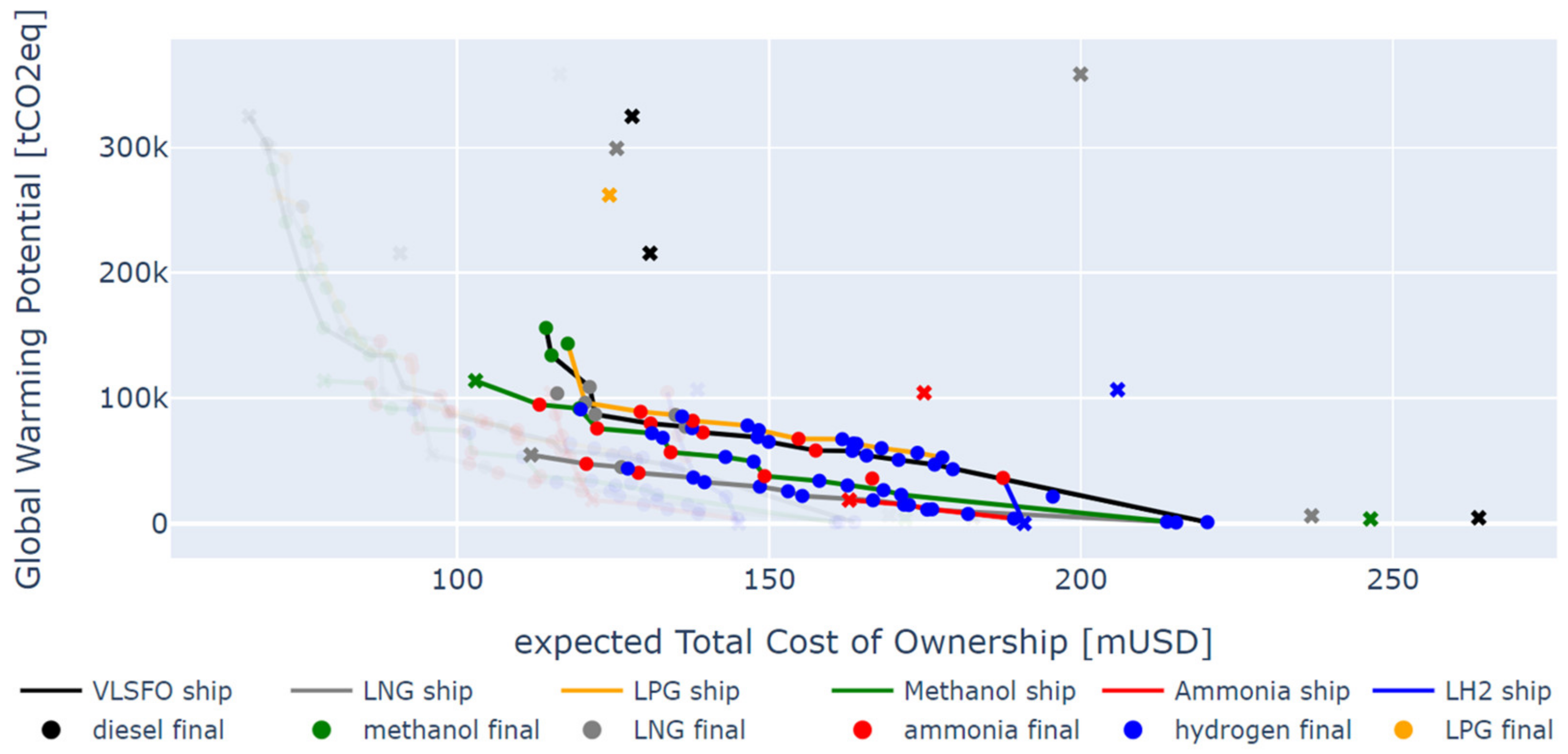
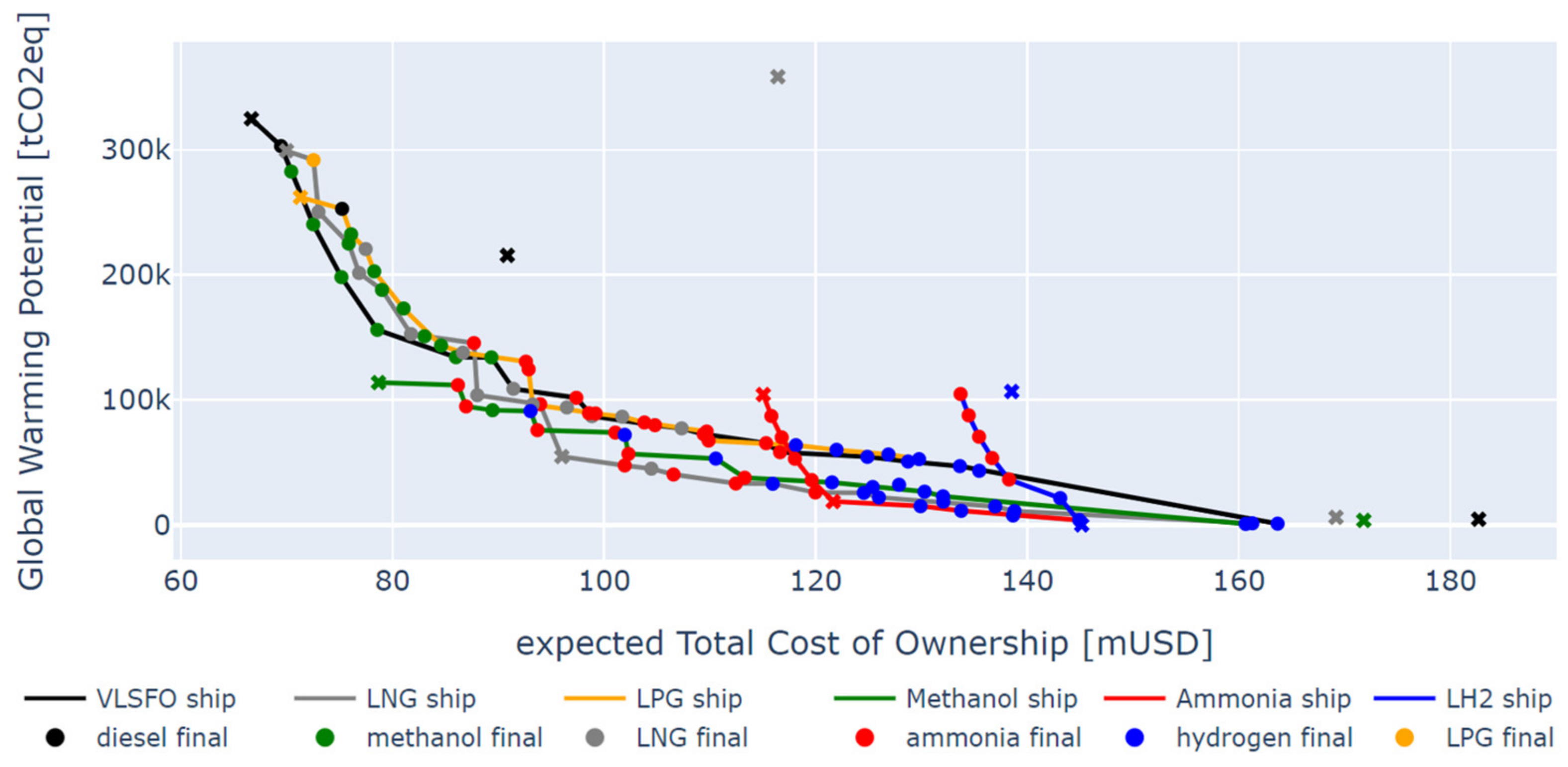
Figure 3 shows the multi-objective Pareto fronts for static (crosses) and flexible solutions when the conservativeness level is as large as the identified uncertainty ranges. The deterministic Pareto fronts are visualized as well.

The large conservativeness against carbon pricing shifts fossil and biofuel options with higher emissions beyond the Pareto front. At lower cost, robust optimization advocates switching focus toward methanol and LNG ships instead, as other vessels are costly and cannot meet reduction targets or need to switch fuels regardless. In addition, ammonia ships still offer a significant GWP reduction at a higher cost. 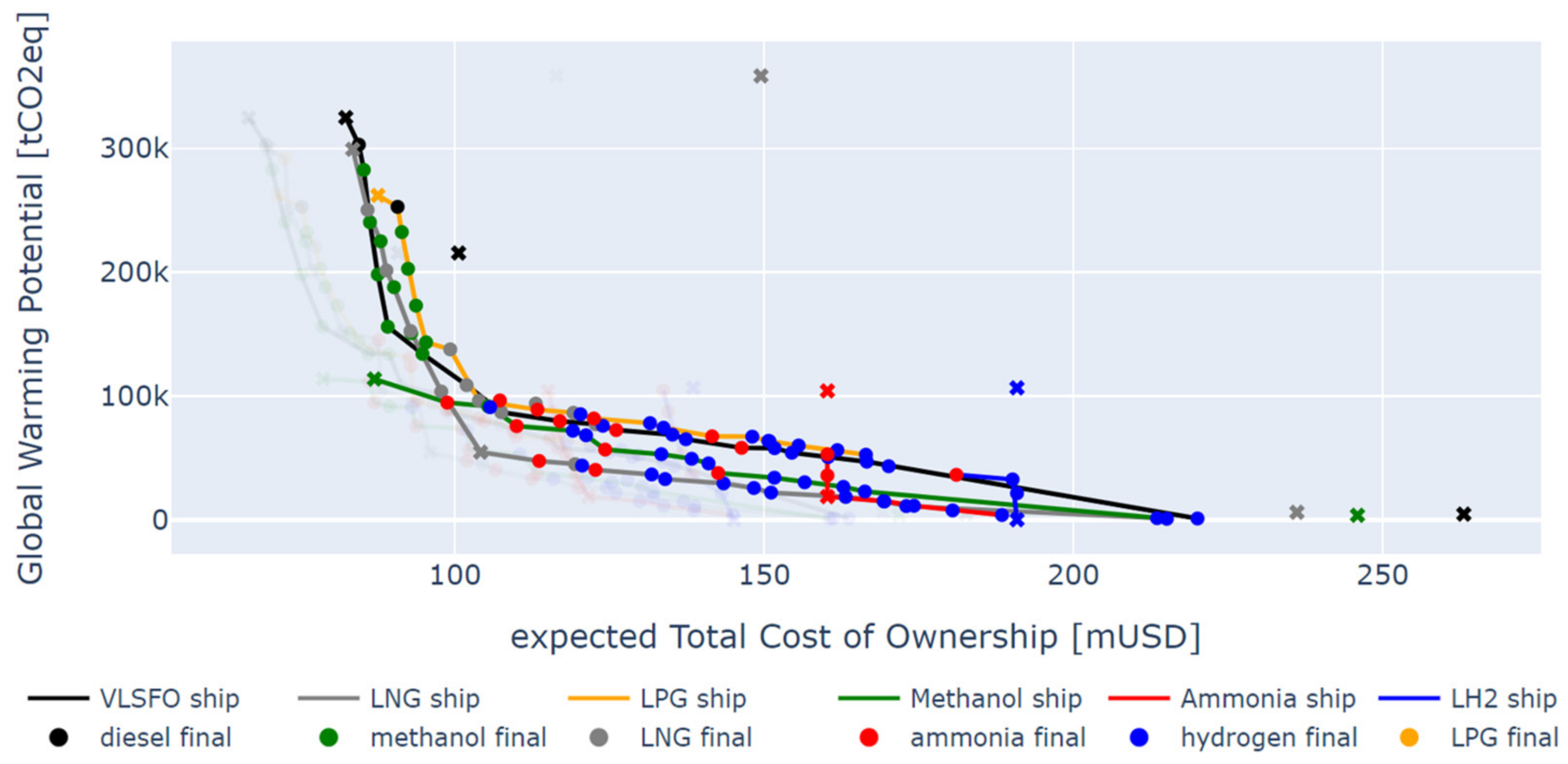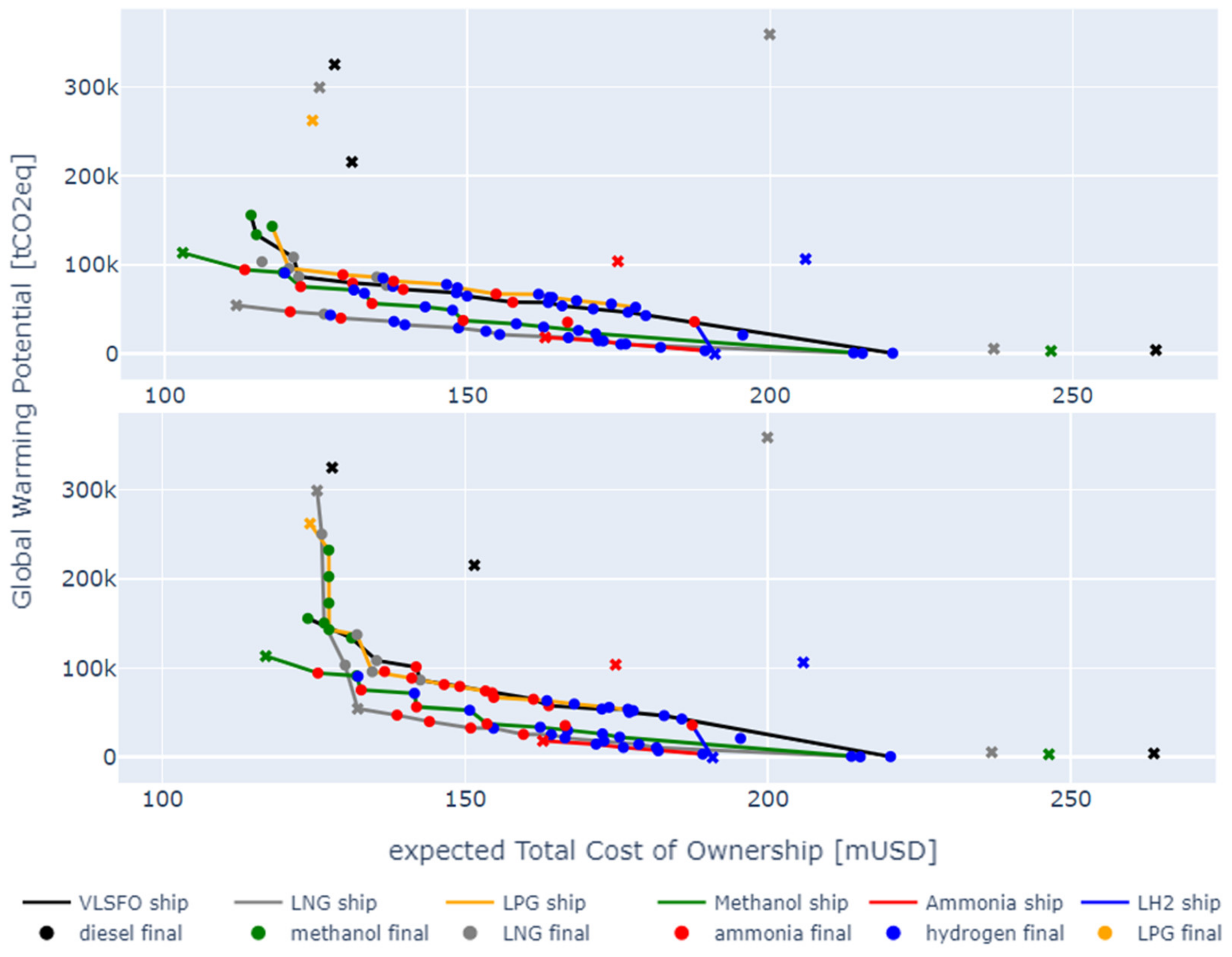To further visualize the impact of fuel price uncertainty, Figure 4 shows results when negating carbon pricing.

When considering only fuel price uncertainty, all options shift to the right. More importantly, the emission reduction slope steepens (reduction becomes cheaper) and the Pareto fronts become more smooth. Furthermore, because there is much uncertainty in the price of ammonia, its TCO shifts to the right, while biofuels like bio-LNG and bio-methanol become more attractive transition options. At medium GWP targets, preference also seems to shift from ammonia toward hydrogen as a final pathway option. This could be explained by the options coming closer together due to high uncertainty, while hydrogen allows initial lenience as it has a higher potential emission reduction. In general, the static options offer cheaper solutions but are not able to adapt toward lower GWP toward the end of the life cycle. When looking at the least cost pathway toward low or zero emissions, primarily ammonia and hydrogen ships are preferred, as other start options imply more expensive retrofits.

4.2.1. Conservativeness Level Selection

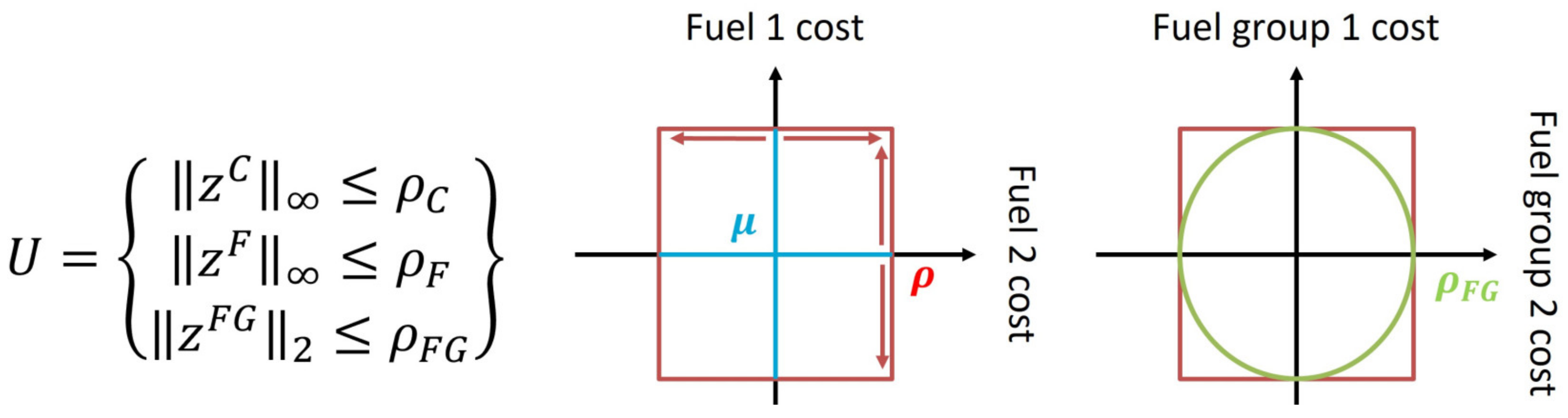
One of the valuable properties of robust optimization is the addition of the conservativeness factor. It allows the decision-maker to select a preferred robustness level. To better understand the impact of conservativeness selection, different values and combinations of ${\rho }_F$ and ${\mathsf{\rho }}_C$ are explored. However, as the additional dimension makes the multi-objective results more difficult to interpret, the GWP objective is rewritten toward two linearized constraints to represent the following reduction targets: 2018 IMO (2050: 50%) and 2020 EU (2030: 40%, 2050: 100%).

First, for the EU target, increasing carbon pricing conservativeness forces owners to switch toward biofuels, while the impact of fuel price uncertainty on the selected start ship and fuel pathway decreases. At low carbon prices, increased conservativeness against fuel prices shows a preference for flexibility to switch between fossil, bio and e-fuels.

Second, for the IMO target, which represents less strict reduction targets, bio-methanol is selected independently of the conservativeness level. Only when being less conservative for carbon and fuel price, the optimization selects cheaper fossil fuels as a start, which have a higher carbon content but a lower price range. More importantly, only for very high carbon price conservativeness (${\mathsf{\rho }}_C=1.5$), the selection is similar to the EU GWP target.

Consequently, carbon pricing primarily affects early pathway decisions, while the GWP target is more impactful regardless of carbon pricing.

Table 6. Single-objective robust optimization solutions for different levels of conservativeness for IMO and EU GWP targets.

		Pathway
Design	Target	Start	2025	2030	2035	2040	2045
0	EU-deterministic	VLSFO ship	VLSFO	Bio-methanol	Bio-methanol	Bio-methanol	E-Ammonia
1	IMO-deterministic	VLSFO ship	VLSFO	Bio-methanol	Bio-methanol	Bio-methanol	Bio-methanol
2	EU-robust	LNG ship	Bio-LNG	Bio-LNG	Bio-LNG	Bio-LNG	Bio-LNG
3	IMO-robust	Methanol ship	Bio-methanol	Bio-methanol	Bio-methanol	Bio-methanol	Bio-methanol

shows the robust selections against the deterministic solutions.

4.2.2. Measurement Criteria: Impact of Conservativeness Selection

Selecting a higher robustness level will result in different starting points. Effectively, the optimization results in three different ships and four different pathways, which are selected dependent on GWP targets and conservatism levels.

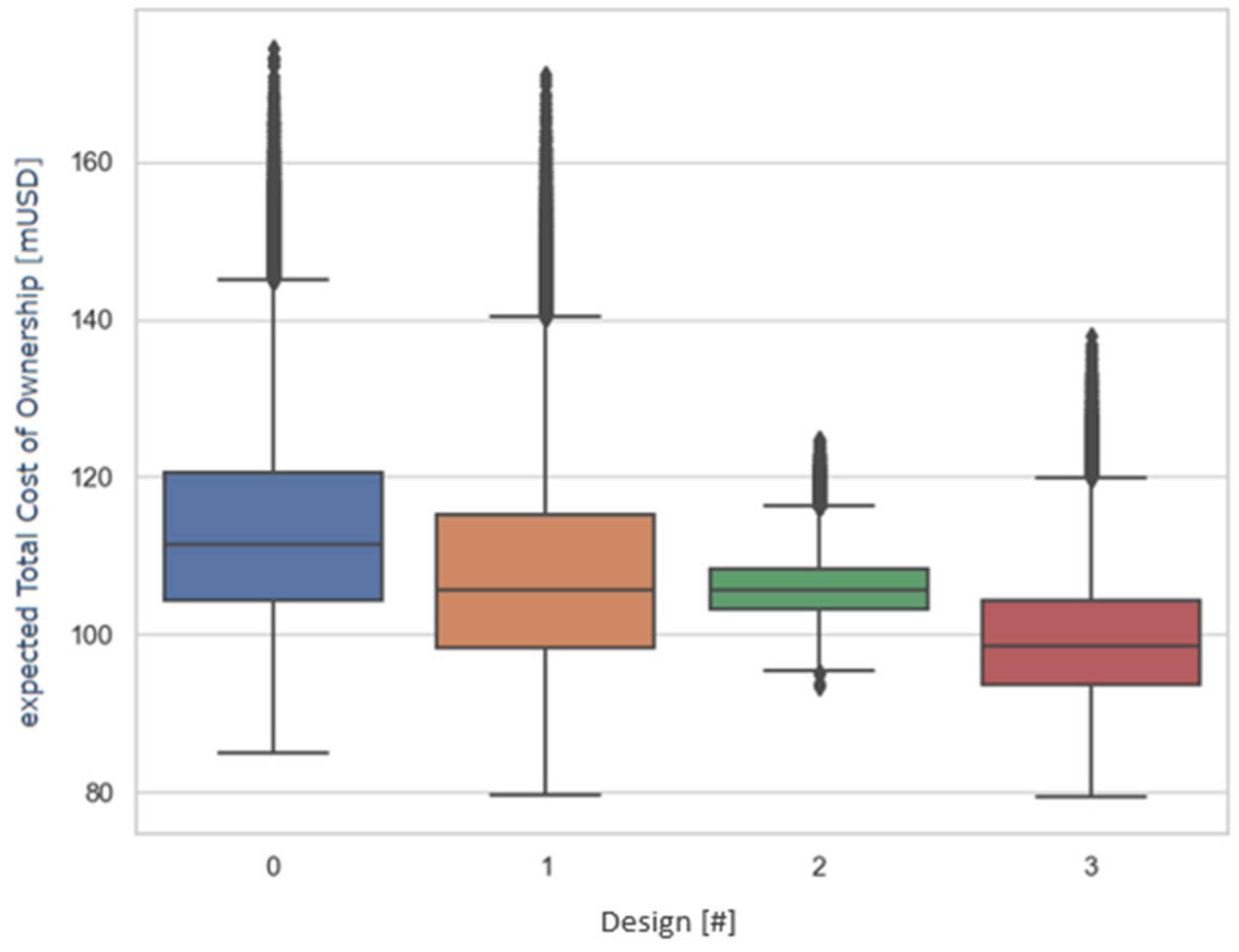
We use the principle of uncertainty quantification [40] to examine the impact of uncertain inputs on the result to see if adaptive robust optimization actually selects robust options. This can be tested by generating a dataset of future scenarios to evaluate the performance of the selections. The sampling is comparable to stochastic optimization, where future prices are sampled from a normal distribution, while carbon price scenarios use a beta-variate distribution. The results of the selected options for 10,000 different sampled futures are shown in Figure 5.

In both cases (designs 2 and 3), the method selects options which have low variance, while the deterministic selection has much larger perturbations. Surprisingly, the robust options seem to prefer a static pathway for each GWP strategy. This can be explained by the variance being so low that retrofit cost becomes a significant investment. Therefore, adaptability seems to be neglected, but its benefit is apparent when looking at the multi-objective figures.

4.2.3. Impact of Changing Variability

Biofuels are found in many pathways on the Pareto fronts. This could be explained by its low variability (15–18%) versus e-fuels (~50%) and fossil fuels (40–60%). However, there are multiple barriers like availability, manufacturing cost and government actions that could increase this variability [41]. Therefore, the variability for biofuels is increased to 50% to examine if the robust optimization selection is impacted. The results for both ranges are presented in Figure 6 for medium carbon price conservativeness (${\mathsf{\rho }}_C=0.5$) and high fuel price conservativeness (${\rho }_F=1$).

There are a few interesting changes due to increased biofuel variability. First, the fronts shift to the right, such that fossil options are in the range of the Pareto fronts, while e-fuel options at lower GWP do not change. More notably, the biofuel shift primarily impacts the mid-range or transition options, where, despite cost increases, biofuels still offer a large reduction potential against a low-cost increase versus fossil fuels. Second, the methanol and LNG ship Pareto shift slightly closer, because the LNG front is found to be more dependent on biofuels. This is also apparent from the heavier focus on ammonia, which is switched to earlier instead of balancing out the GWP from cheaper bio-LNG by switching to hydrogen later on. Nevertheless, even though pathways are impacted, start ship decisions (Pareto fronts) seem to be unaffected by variability changes. More importantly, this shows that there is significant value in being able to retrofit to deal with uncertainty after having selected a starting point.

4.2.4. Discussion

Robust optimization was shown to be able to select a set of robust solutions from a large number of options. Furthermore, in the case of alternative fuel selection, switching fuels during the lifetime can be included by using adaptive robust optimization. It can be used to understand the adaptability gap, which is the difference between the static (fixed case) and adaptive robust solution (flexible case). Robust optimization methods shift the focus of a decision-maker from one assumed value toward properly establishing an uncertainty range by adding conservativeness. However, although this allows the decision-maker to immunize against the selected uncertainty, the solution can become too conservative. This can be dealt with in two ways: the correlation can be changed using a different uncertainty set, or the conservative factor itself can be reduced. The impact of uncertainty sets has been discussed extensively in the literature [19], while this paper primarily discussed the conservativeness factor selection. The impact of these is preferably explored, but this is found to be difficult due to the increased dimensionality. However, a big advantage of robust optimization against other methods is its tractability. This allows the number of uncertain parameters to be increased against low computational cost. Overall, the addition of uncertain parameters for ship design works well with single and multi-objective optimization, but sensitivity exploration is more complex.

4.3. Stochastic Optimization

This subsection will briefly present the results obtained from the stochastic model. Section 4.3.1 presents the results from the base case as described in Section 3. Section 4.3.2 describes the value of a stochastic solution, and Section 4.3.3 discusses the results when adjusting the bounds for biofuels.

4.3.1. Stochastic Optimization Base Case

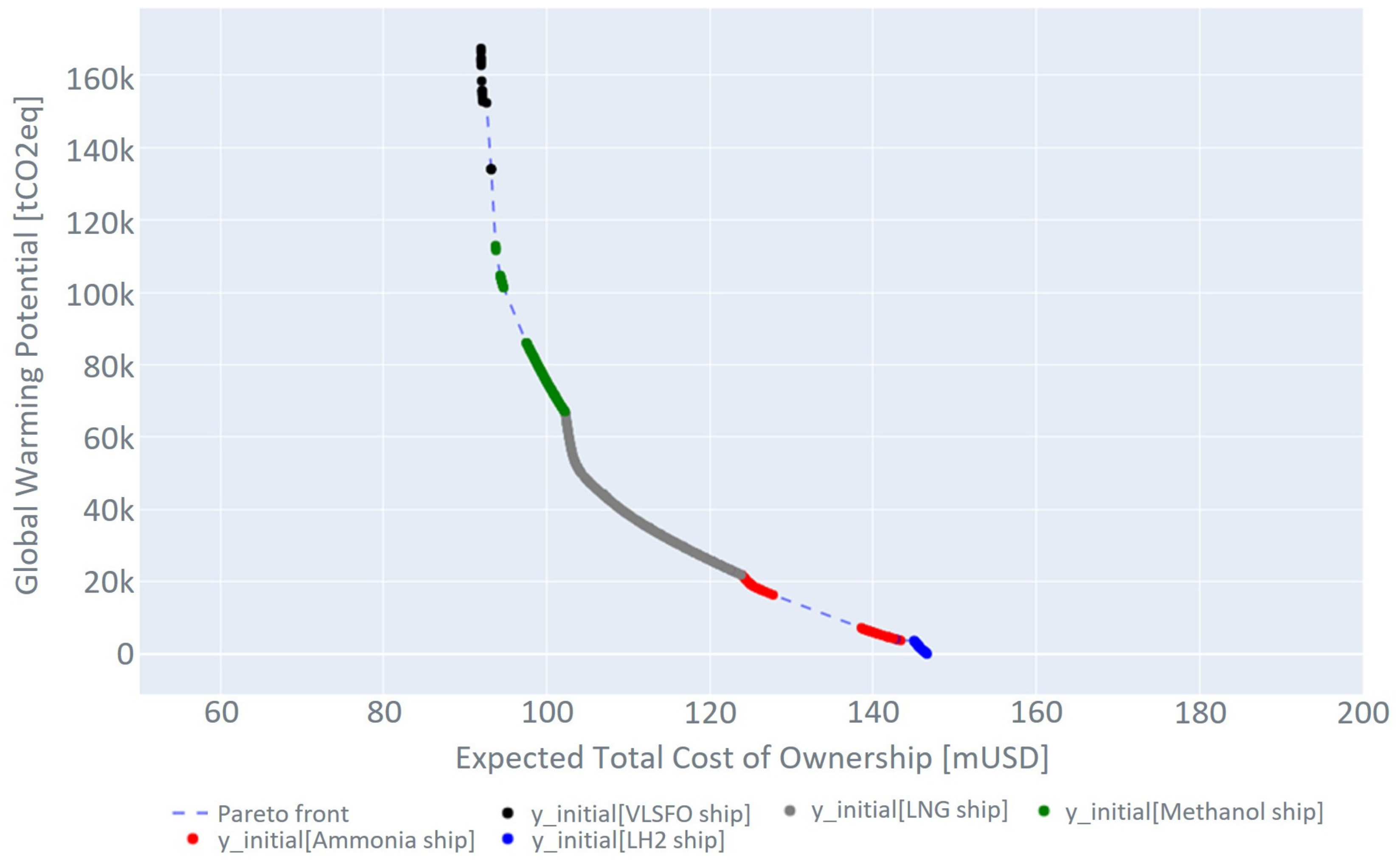
The Pareto front of solutions from the stochastic optimization is shown in Figure 7. The plot shows that the expected emissions can be lowered by roughly 50% for a marginal increase in expected costs. Reducing emissions all the way down to zero would result in an approximately 60% increase in the expected costs.

In terms of optimal power system choice for the new build, methanol is suggested as a favorable abatement option for up to 60% emission reduction, while an LNG power system would optimal between 60% and 90% reduction. Abating the last 10% of emissions would require ammonia or hydrogen configurations from the beginning.

4.3.2. Value of Stochastic Solution

The Value of the Stochastic Solution (VSS) characterizes the cost delta between implementing the first-stage decisions of a deterministic program based on expected values vs. implementing the first-stage decisions of the stochastic program. That is, the optimal first-stage decisions of the deterministic expected value formulation are simulated under the stochastic setting.

As for this case study, Lagemann et al. [17] have found that the VSS expressed in monetary terms is generally low. That means that the first-stage decisions suggested by the deterministic expected value problem do not perform much worse than the first-stage decisions suggested by the stochastic model. However, the suggested first-stage decisions in the deterministic problem alternate frequently with the decreasing target GWP. This feature is not present in the stochastic solution. Thus, the deterministic solution suggests artificial chaos, which is not present in the data but rather stems from the discreteness of the problem. More precisely, it is the limited number of possible combinations that generate this alternation of optimal first-stage decisions. The VSS in this case could be better measured as “insight produced”.

4.3.3. Stochastic Model with Adjusted Bounds for Biofuels

In Section 4.2, we have shown that the results of the base case might be biased due to the low variability in biofuel prices. In order to investigate a change in bounds, we keep the lower bound as is and adjust the upper bound such that the difference between the original mean/mode is now 50%, as for most other fuels. As a result, the triangular distribution becomes asymmetric, with the mode assumed as the original mean, and the new mean is higher due to the adjusted upper bound. Pantuso et al. [42] have shown that stochastic programs are often relatively insensitive to the actual probability distributions while being sensitive to the mean. We will discuss this hypothesis in the light of this case study.

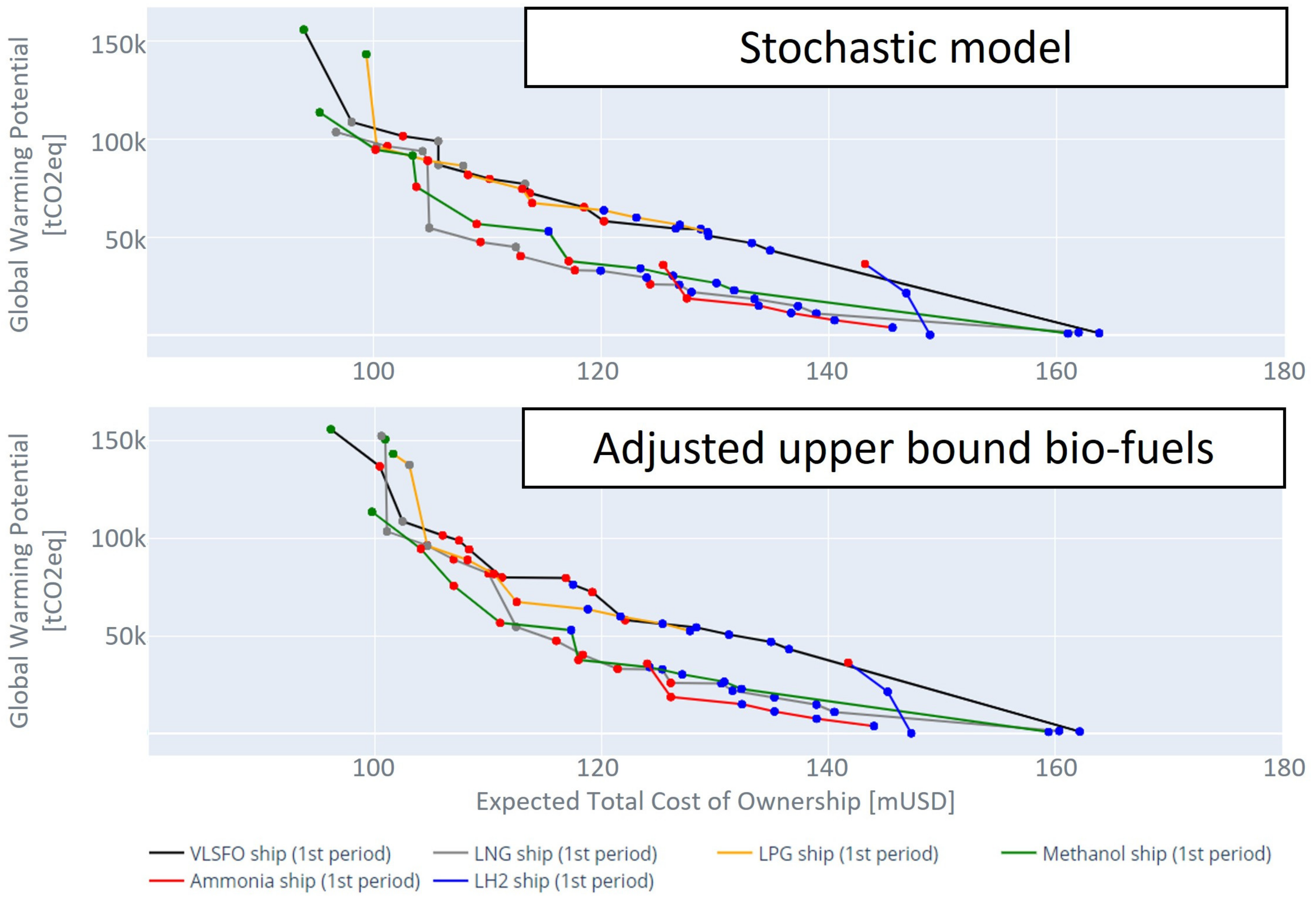
When plotting the suggested first-stage decisions, i.e., what initial system to invest in, there is little difference to observe in the Pareto front. The effect of adjusted upper bounds for biofuels differs, however, when it comes to retrofits. This can be seen in Figure 8, which uses a brute force technique. That is, it traces fixed combinations of fuels and systems over time across the same scenario set as the optimization model. The line’s color indicates the first-stage decision (the initial system), while the dot’s color indicates the final system in the last period. This technique has shown to yield relevant insight [17].

Applying the brute force technique to the adjusted biofuels brings to the surface some secondary effects, namely potential retrofits: retrofits toward ammonia become more frequent along the Pareto front for adjusted biofuel bounds, while retrofits toward hydrogen are less frequent. Our hypothesis for this is that adjusting the upper bound for biofuels naturally renders them more expensive. The model thus is inclined to switch earlier to e-fuels, for which the retrofit to ammonia is cheaper.

4.3.4. Stochastic Optimization Discussion

Stochastic optimization offers the ability to balance optimization by weighting uncertain outliers stochastically. In this way, the method allows selecting from many options while taking uncertainty into account explicitly. Furthermore, by using two-stage stochastic optimization, the method is able to separate the problem into initial (here-and-now) and future (wait-and-see) decisions. This shall reflect the position of a shipowner today because it models the future to be unfolding only after the initial selection. The use of probability shifts the focus of decision-makers toward identifying distributions instead of single values and allows for specifying a nuanced belief in the likelihood of scenarios. Nevertheless, one still needs to specify these probability distributions explicitly, which is challenging especially for high uncertainty levels. In the case of additional uncertainties, the probability distributions can possibly lead to a non-convexity of the problem. Even though several approaches exist to deal with non-convex stochastic optimization problems [43,44], such mathematical limitations must be kept in mind for future extensions and adaptions. Robust optimization was shown to be able to select a set of robust solutions from a large number of options.

4.4. Discussion across Methods

By applying both methods to the same problem, the output, methodological assumptions and impact for this specific use case can be compared. When comparing the methods to the deterministic solution, it is apparent that taking uncertainty into account results in different selections, which focus on improving robustness while also incorporating the value of flexibility. The following paragraphs each comment on one of our initially stated aspects for comparison.

Looking at the representation of uncertainty, either conservativeness factors or stochastic distributions are used. However, despite a different approach, the fronts offer very similar insights. On the one hand, for robust optimization, the impact of robustness is clarified when it is compared to the deterministic solution. While on the other hand, stochastic optimization offers smoother Pareto fronts and is less dependent on the initial solution.

Regarding insight for ship designers, it is shown that the conservativeness values in robust optimization offer much freedom to research different scenarios, even though it increases the dimensionality of the problem. Otherwise, stochastic optimization is more static, but it has several criteria that offer detailed insights on the difference against the deterministic solution.

To research the sensitivity of assumptions, the variability and probability distribution were changed for biofuel. Robust optimization was found to be sensitive to increasing variability, while the selection of the mean is more impactful when using stochastic optimization. Overall, in this case study, these impacts are primarily found at the pathway levels and ending option, respectively, while the start selections remain similar. When comparing recommendations from each method, outcomes are very similar, especially regarding the optimal start ship.

Table 7. Advantages and disadvantages of the two optimization methods.

Method	Pros	Cons
Robust optimization	Takes uncertainty into account in modelling stage	Can become too conservative
	Immunizes against uncertainty	Uncertainty set and conservativeness selection
	Adaptive robust decision making	Dimensionality due to added factors
	Very tractable: low cost extension to multiple uncertainties
Stochastic optimization	Risk is taken care of explicitly	Probability distribution difficult to specify reliably
	Wait-and-see and here-and-now decisions	Probability can make the problem nonconvex and difficult to solve
	Can treat extreme scenarios as unlikely using low probability	Too large to solve with multiple uncertainties

further summarizes the pros and cons of each method while showing the aspects that are deemed to be of specific importance for this case study in bold.

The setup of the MILP and collecting reliable input was found to be more demanding than subsequently constructing either method. Therefore, in our opinion, the difficulty of implementation primarily depends on the choice to use optimization rather than the choice between robust and stochastic methods. Nonetheless, for robust optimization, the uncertainty set and conservativeness level selection effort proved significant, while for stochastic optimization, the computational effort, due to the use of probability and sampling, is more pressing. Above all, besides the insights from the method output, the knowledge gained through structuring such a problem is deemed to be especially valuable in the face of uncertainty.

5. Conclusions

Robust and stochastic optimization methods are found to present similar solutions for the selected uncertainties under the same assumed input conditions. Robust optimization offers more extensive scenario research capabilities by using different conservativeness levels and uncertainty sets. However, its results are more readable compared to a deterministic solution, while they were found to be primarily sensitive to variability changes in the uncertainty set. Stochastic optimization provides smoother fronts with fewer alternations, while it offers several criteria to gain more detailed insights into the difference against a deterministic solution. Its results are primarily impacted by the selection of the mean of the probability distribution. The required computational effort is more significant in particular for larger scenario sets. By using both methods, it is found that confidence in final solutions can be improved and additional insights can be gained.

For the selection of alternative fuel and power systems, the success of these methods primarily depends on the level of uncertainty and ability to set up the input for each method. Nevertheless, both methods shift attention toward defining either probabilistic or conservativeness factors and encourage the decision-maker to consider uncertainty in the problem explicitly. As demonstrated, many different uncertainties can impact the results in a decision problem such as maritime energy carrier selection. While this paper only looked into two uncertainties, much more are preferably included in the decision problem. An extension of uncertain factors should be covered in further research. For this purpose, robust optimization seems to be promising due to its tractability, but this remains to be proven.

From a more practical standpoint, the methods show that methanol and LNG ships allow a cheap but large reduction in emissions through the use of biofuels. However, flexibility is key for these options to be able to follow possible shifts in fuel or carbon prices as modeled in this paper. The ability to switch toward other fuels during the lifetime was found to become even more important for values that occur outside of the assumed ranges. This was shown for a potential variability change for biofuels, which was still selected as an important intermediate solution for emission reduction despite the shift of the mean and the increase in the price range.

Consequently, under the conditions of the case study, including uncertainty in such a selection problem is more important than the choice of a specific method. Furthermore, applying both methods to the same dataset can increase confidence in the practical results. We have shown that the suggested decisions of both methods are very similar. Thus, the choice of method, in our case, affects the decisions to a much lesser extent than the assumptions made for the input parameters. Further research should be conducted on different case studies to corroborate or refute the benefit of flexibility and opportunities of biofuels. This paper indicates that the application of fuel selection methods for any ship to meet the IMO emission goals can benefit from including life cycle uncertainty.

References

1. CE Delft. Fourth IMO GHG Study; CE Delft: Delft, The Netherlands, 2020. [Google Scholar]
2. United Nations. Paris Agreement. 2015. Available online: https://unfccc.int/process-and-meetings/the-paris-agreement (accessed on 30 November 2022).
3. International Maritime Organization. Resolution MEPC.377(80); IMO: London, UK, 2023. [Google Scholar]
4. Bouman, E.A.; Lindstad, E.; Rialland, A.I.; Strømman, A.H. State-of-the-art technologies, measures, and potential for reducing GHG emissions from shipping—A review. Transp. Res. Part D Transp. Environ. 2017, 52, 408–421. [Google Scholar] [CrossRef]
5. DNV. Maritime Forecast to 2050. 2022. Available online: https://www.dnv.com/maritime/publications/maritime-forecast-2023/index.html (accessed on 30 November 2022).
6. Lindstad, E.; Gamlem, G.; Rialland, A.; Valland, A. Assessment of Alternative Fuels and Engine Technologies to Reduce GHG. In Proceedings of the SNAME Maritime Convention, Providence, RI, USA, 27–29 October 2021. [Google Scholar]
7. DNV GL. Assessment of Selected Alternative Fuels and Technologies; DNV: Høvik, Norway, 2019. [Google Scholar]
8. Korberg, A.; Brynolf, S.; Grahn, M.; Skov, I. Techno-economic assessment of advanced fuels and propulsion systems in future fossil-free ships. Renew. Sustain. Energy Rev. 2021, 142, 110861. [Google Scholar] [CrossRef]
9. Lloyd’s Register and UMAS. Techno-Economic Assessment of Zero-Carbon Fuels. 2020. Available online: https://www.methanol.org/techno-economic-assessment-of-zero-carbon-fuels/ (accessed on 30 November 2022).
10. Wu, Y.; Zhang, H.; Li, F.; Wang, S.; Zhen, L. Optimal Selection of Multi-Fuel Engines for Ships Considering. Mathematics 2023, 11, 3621. [Google Scholar] [CrossRef]
11. Niese, N.D.; Kana, A.A.; Singer, D.J. Ship design evaluation subject to carbon emission policymaking using a Markov decision process framework. Ocean Eng. 2015, 106, 371–385. [Google Scholar] [CrossRef]
12. Ship & Bunker. FEATURE: 10 Years of Bunker Prices. 16 June 2022. Available online: https://shipandbunker.com/news/world/366958-feature-10-years-of-bunker-prices (accessed on 30 November 2022).
13. De Neufville, R.; Scholtes, S. Flexibility in Engineering Design; The MIT Press: Cambridge, MA, USA, 2019. [Google Scholar]
14. Haneveld, W.K.K.; van der Vlerk, M.H.; Romeijnders, W. Stochastic Programming: Modelling Decision Problems under Uncertainty; Springer: Berlin/Heidelberg, Germany, 2020. [Google Scholar]
15. Bertsimas, D.; den Hertog, D. Robust Optimization; Dynamic Ideas: Belmont, MA, USA, 2022. [Google Scholar]
16. Lagemann, B.; Lindstad, E.; Fagerholt, K.; Rialland, A.; Erikstad, S.O. Optimal ship lifetime fuel and power system selection. Transp. Res. Part D Transp. Environ. 2022, 102, 103145. [Google Scholar] [CrossRef]
17. Lagemann, B.; Lagouvardou, S.; Lindstad, E.; Fagerholt, K.; Psaraftis, H.; Erikstad, S.O. Optimal selection of lifetime fuel and power system under uncertainty. Transp. Res. Part D Transp. Environ. 2023, 119, 103748. [Google Scholar] [CrossRef]
18. Ben-Tal, A.; El Ghaoui, L.; Nemirovski, A. Robust Optimization; Princeton University Press: Princeton, NJ, USA, 2009. [Google Scholar]
19. Gabrel, V.; Murat, C.; Thiele, A. Recent advances in robust optimization: An overview. Eur. J. Oper. Res. 2014, 28, 471–483. [Google Scholar] [CrossRef]
20. Zhang, Y.; Yiping, F.; Gang, R. New robust optimization approach induced by flexible uncertainty set: Optimization under continuous uncertainty. Ind. Eng. Chem. Res. 2017, 56, 270–287. [Google Scholar] [CrossRef]
21. Chen, X.; Melvyn, S.; Peng, S. A robust optimization perspective on stochastic programming. Oper. Res. 2007, 55, 1058–1071. [Google Scholar] [CrossRef]
22. Ben-Tal, A.; Bertsimas, D.; Brown, D.B. A soft robust model for optimization under ambiguity. Oper. Res. 2010, 58, 1220–1234. [Google Scholar] [CrossRef]
23. Bertsimas, D.; Goyal, V. On the power of robust solutions in two-stage stochastic and adaptive optimization problems. Math. Oper. Res. 2010, 35, 284–305. [Google Scholar] [CrossRef]
24. Ramsay, W.J.; Fridell, E.; Michan, M. Maritime Energy Transition: Future Fuels & Future Emissions. J. Mar. Sci. Appl. 2022, 22, 681–692. [Google Scholar]
25. Kouzelis, K.; Koos, F.; van Hassel, E. Maritime fuels of the future: What is the impact of alternative fuels on the optimal economic speed of large container vessels. J. Shipp. Trade 2022, 7, 23. [Google Scholar] [CrossRef]
26. Zhao, Y.; Ye, J.; Zhou, J. Container fleet renewal considering multiple sulfur reduction technologies and uncertain markets amidst COVID-19. J. Clean. Prod. 2019, 317, 128361. [Google Scholar] [CrossRef]
27. Lindstad, E.; Lagemann, B.; Rialland, A.; Gamlem, G.M.; Valland, A. Reduction of maritime GHG emissions and the potential role of E-fuels. Transp. Res. Part D Transp. Environ. 2021, 101, 103075. [Google Scholar] [CrossRef]
28. Haehl, C.; Spinler, S. Technology Choice under Emission Regulation Uncertainty in International Container Shipping. Eur. J. Oper. Res. 2020, 284, 383–396. [Google Scholar] [CrossRef]
29. Bergsma, J.M.; Pruyn, J.; van de Kaa, G. A Literature Evaluation of Systemic Challenges Affecting the European Maritime Energy Transition. Sustainability 2021, 13, 715. [Google Scholar] [CrossRef]
30. Wahl, J.; Kallo, J. Carbon abatement cost of hydrogen based synthetic fuels–A general framework exemplarily applied to the maritime sector. Int. J. Hydrogen Energy 2022, 47, 3515–3531. [Google Scholar] [CrossRef]
31. Grahn, M.; Malmgren, E.; Korberg, A.; Taljegard, M.; Anderson, J.; Brynolf, S.; Hansson, J.; Skov, I.; Wallington, T. Review of electrofuel feasibility-Cost and environmental impact. Prog. Energy 2022, 4, 032010. [Google Scholar] [CrossRef]
32. Ros, J.A.; Skylogianni, E.; Doedée, V.; van den Akker, J.T.; Vredeveldt, A.W.; Linders, M.J.; Goetheer, E.L.; Monteiro, J.G. Advancements in ship-based carbon capture technology on board of LNG-fuelled ships. Int. J. Greenh. Gas Control 2022, 114, 103575. [Google Scholar] [CrossRef]
33. Achtnicht, M.; Buhler, G.; Hermeling, C. The impact of fuel availability on demand for alternative-fuel vehicles. Transp. Res. Part D Transp. Environ. 2012, 17, 262–269. [Google Scholar] [CrossRef]
34. Prussi, M.; Yugo, M.; De Prada, L.; Padella, M.; Edwards, R.; Lonza, L. JEC Well-to-Tank Report v5; Publications Office of the European Union: Luxembourg, 2022. [Google Scholar]
35. Wang, Y.; Wright, L.A. A Comparative Review of alternative Fuels for the Maritime Sector: Economic, Technology, and Policy Challenges for Clean Energy Implementation. World 2021, 2, 456–481. [Google Scholar] [CrossRef]
36. Serra, P.; Fancello, G. Towards the IMO’s GHG goals: A critical overview of the perspectives and challenges of the main options for decarbonizing international shipping. Sustainability 2020, 12, 3220. [Google Scholar] [CrossRef]
37. Lagouvardou, S.; Psaraftis, H.N.; Zis, T. A Literature Survey on Market-Based Measures for the Decarbonization of Shipping. Sustainability 2020, 12, 3953. [Google Scholar] [CrossRef]
38. Kass, M.; Sluder, C.; Kaul, B. Spill Behavior, Detection, and Mitigation for Emerging Nontraditional Marine Fuels; Oak Ridge National Laboratory: Oak Ridge, TN, USA, 2021. [Google Scholar]
39. Sustainable Shipping Initiative. The role of sustainable biofuels in the decarbonization of shipping: The findings of an inquiry into the sustainability and availability of biofuels for shipping. In Proceedings of the United Nations Climate Change Conference, COP25, Madrid, Spain, 11 December 2019. [Google Scholar]
40. Scarabosio, L. Quantifying Uncertainty: Prediction and Inverse Problems; Radboud Summer School: Nijmegen, The Netherlands, 2022. [Google Scholar]
41. Kesieme, U.; Pazouki, K.; Murphy, A.; Chrysanthou, A. Biofuel as an alternative shipping fuel: Technological, environmental and economic assessment. Sustain. Energy Fuels 2019, 3, 899–909. [Google Scholar] [CrossRef]
42. Pantuso, G.; Fagerholt, K.; Wallace, S.W. Which uncertainty is important in multistage stochastic programmes? A case from maritime transportation. IMA J. Manag. Math. 2015, 28, 5–17. [Google Scholar] [CrossRef]
43. Liu, A.; Lau, V.K.N.; Kananian, B. Stochastic Successive Convex Approximation for Non-Convex Constrained Stochastic Optimization. IEEE Trans. Signal Process. 2019, 67, 4189–4203. [Google Scholar] [CrossRef]
44. Arjevani, Y.; Carmon, Y.; Duchi, J.C.; Foster, D.J.; Srebro, N.; Woodworth, B. Lower bounds for non-convex stochastic optimization. Math. Program. 2022, 199, 165–214. [Google Scholar] [CrossRef]
Figure 1. Uncertainty set visualization.
Sustainability 16 01947 g001
Figure 2. Multi-objective plot for the deterministic case with mean fuel prices and 0 carbon price. The colored crosses are non-flexible solutions that stick to a single fuel, and colored lines identify the start system and lowest GWP pathway of a flexible ship. The same result was found for both the robust and stochastic optimization codes. By using deterministic optimization, a decision-maker can already gain an understanding of the potential price to reduce emissions including the starting ship and pathway that could be followed to meet these targets. However, as values might change, do these results hold under uncertain conditions?
Sustainability 16 01947 g002
Figure 3. Multi-objective plot for the robust optimization case with high conservativeness level against the deterministic case in the background.
Sustainability 16 01947 g003
Figure 4. Multi-objective plot for the robust optimization case with zero carbon price and high fuel price conservativeness.
Sustainability 16 01947 g004
Figure 5. Single-objective robust optimization solutions for different levels of conservativeness for IMO and EU GWP targets.
Sustainability 16 01947 g005
Figure 6. Results for original (above) and increased biofuel prices (below).
Sustainability 16 01947 g006
Figure 7. Pareto front for initial power system configurations, 100 scenarios with a stochastic carbon price.
Sustainability 16 01947 g007
Figure 8. Adjusted upper bound for biofuels, brute force results. The color of the lines denotes the initial system that is selected in the first time period. The color of the dots denotes the system that is selected in the last time period.
Sustainability 16 01947 g008