


Analyzing the Impact of COVID-19 on Economic Sustainability: A Clustering Approach


Abstract
1. Introduction
2. Literature Review
3. Methods
3.1. Data Sample
- Banking Sector: This level includes operational continuity, integrity, support for borrowers, prudential regulations, and crisis management strategies.
- Financial Markets/Non-Bank Financial Institutions (NBFIs): This level addresses measures related to non-bank financial institutions (NBFIs), public debt management, and market functioning.
- Insolvency Frameworks: This level encompasses enhancing tools for out-of-court debt restructuring and workouts, amending bankruptcy filing obligations, and other insolvency-related measures.
- Liquidity/Funding Mechanisms: This level comprises policy rate adjustments, asset purchases, liquidity provisions (including foreign exchange/ELA), and other liquidity-related measures.
- Payment Systems Infrastructure: This level includes easing regulatory requirements, promoting and ensuring the availability of digital payment mechanisms, consumer protection measures, ensuring the availability and acceptance of cash, and other payment system-related measures.
3.2. Clustering
3.3. Number of Clusters Estimation Methods
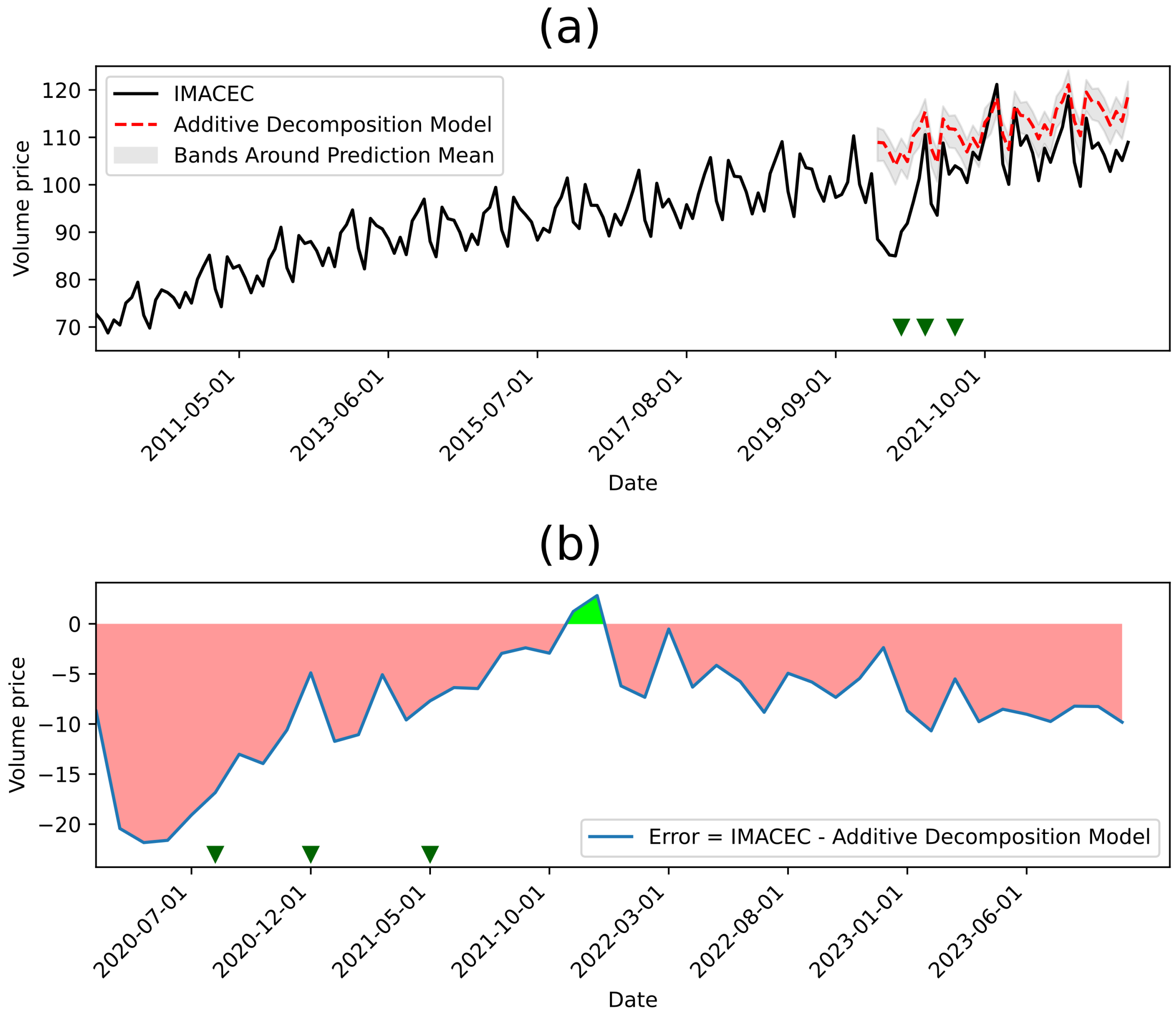
3.4. IMACEC Modelling
4. Results
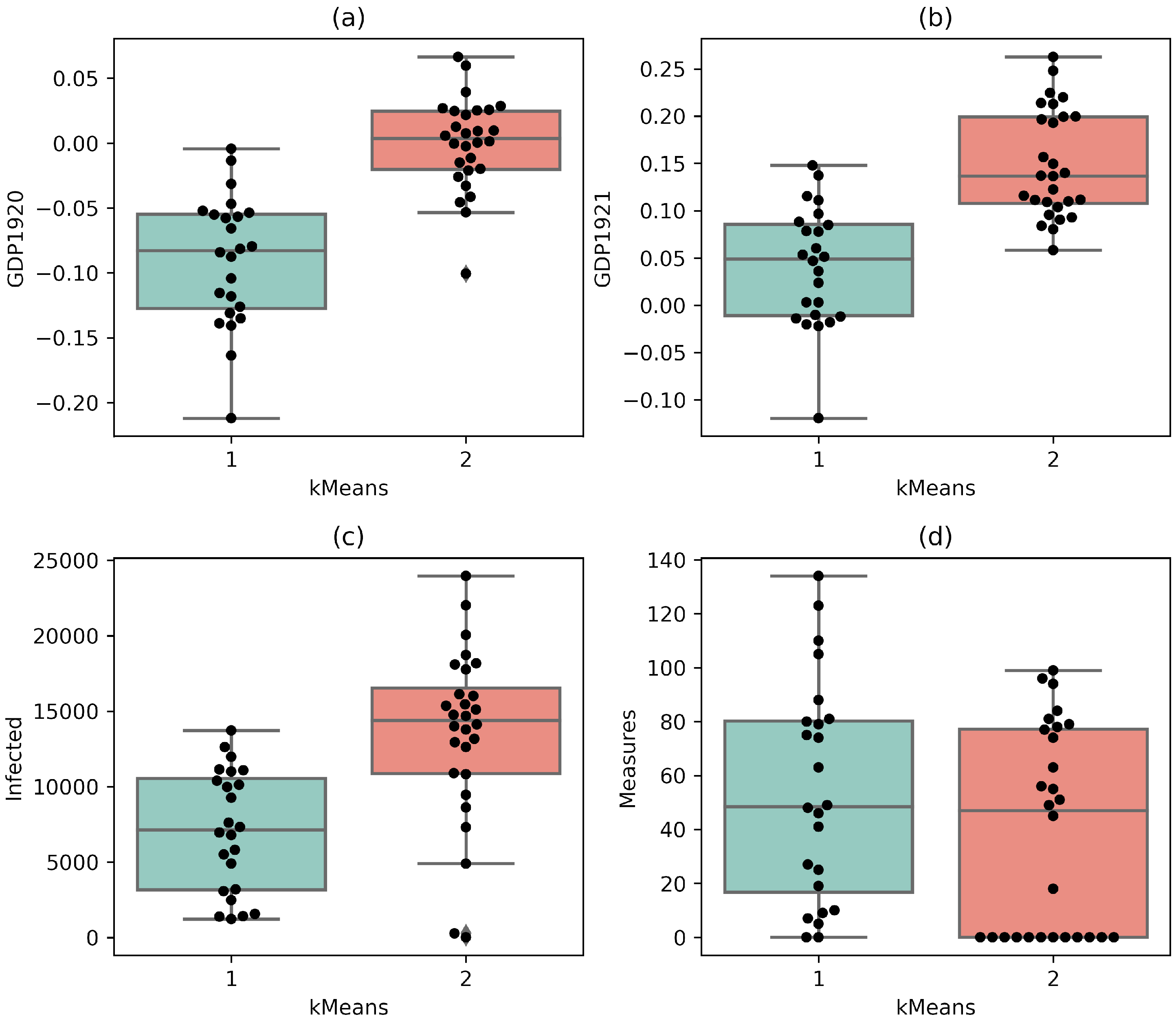
4.1. Exploratory Data Analysis
4.2. Selection of the Number of Clusters
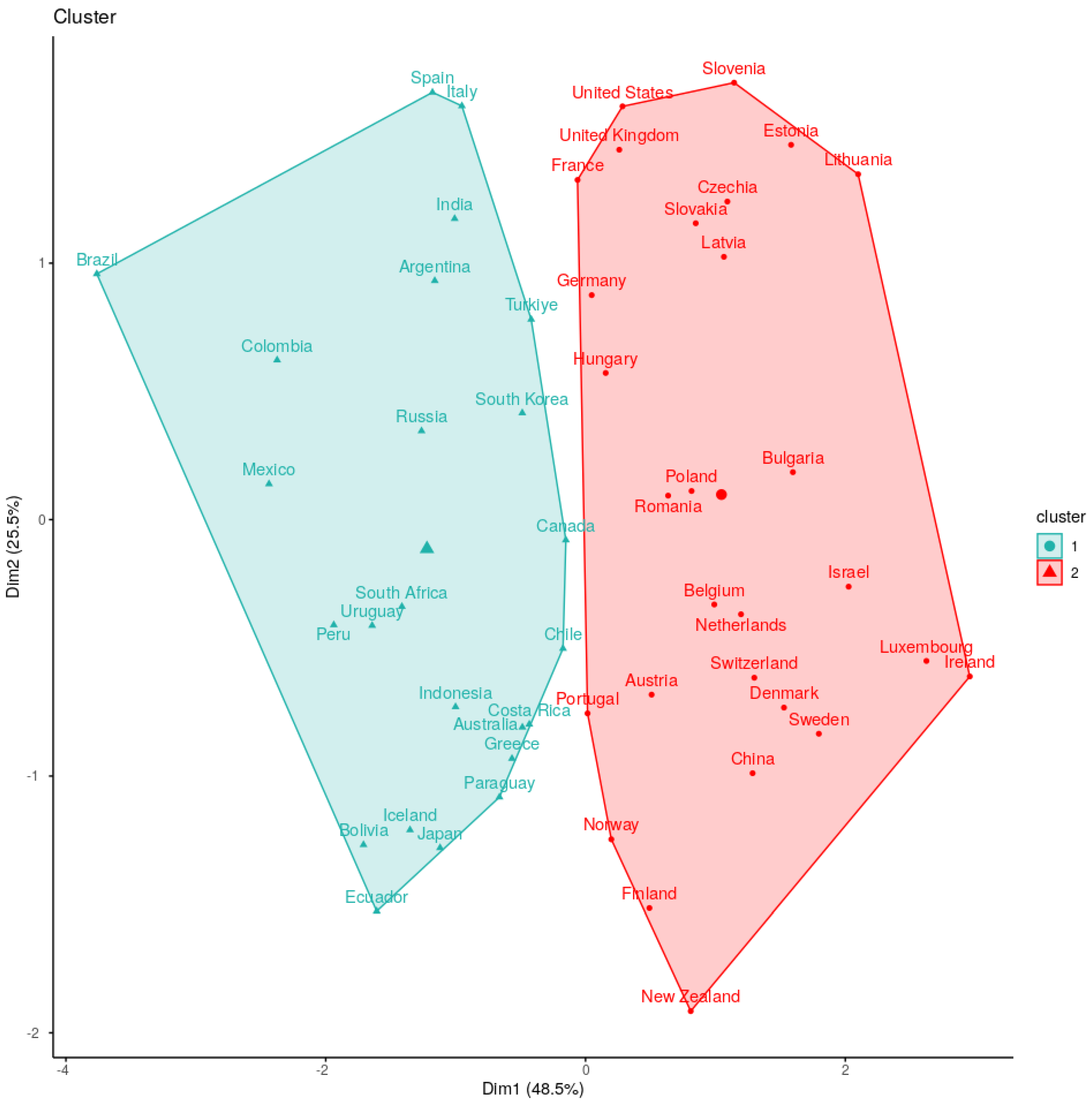
4.3. Formation of Two Significant Clusters Using Static Data from Countries
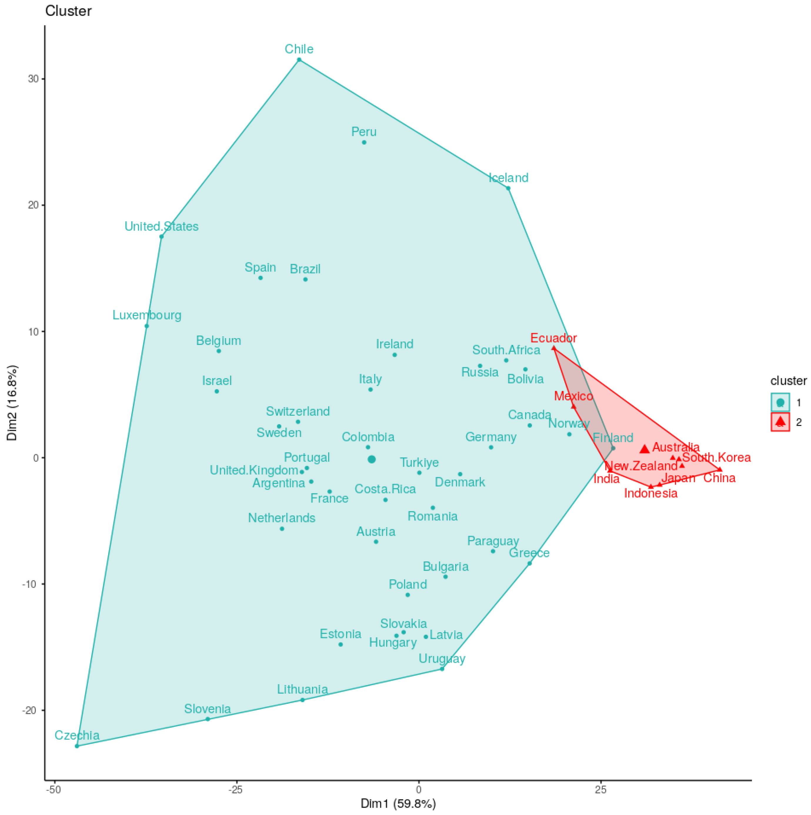
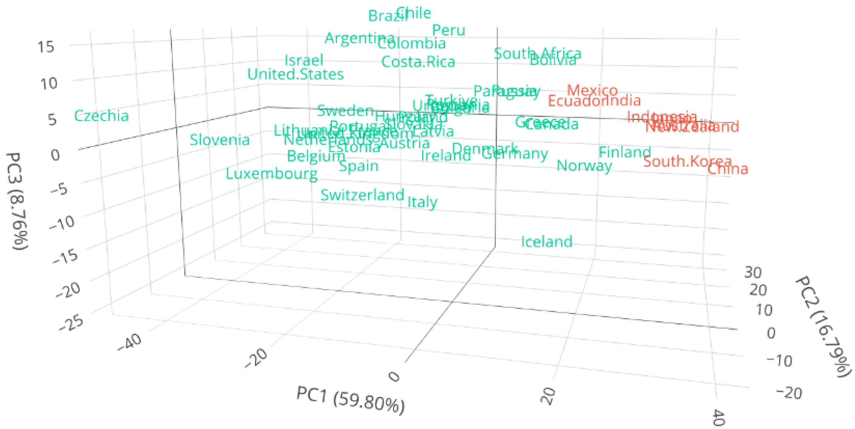
4.4. Clustering the Evolution of Infection Rates in Countries Using Dynamic Time Warping (DTW)
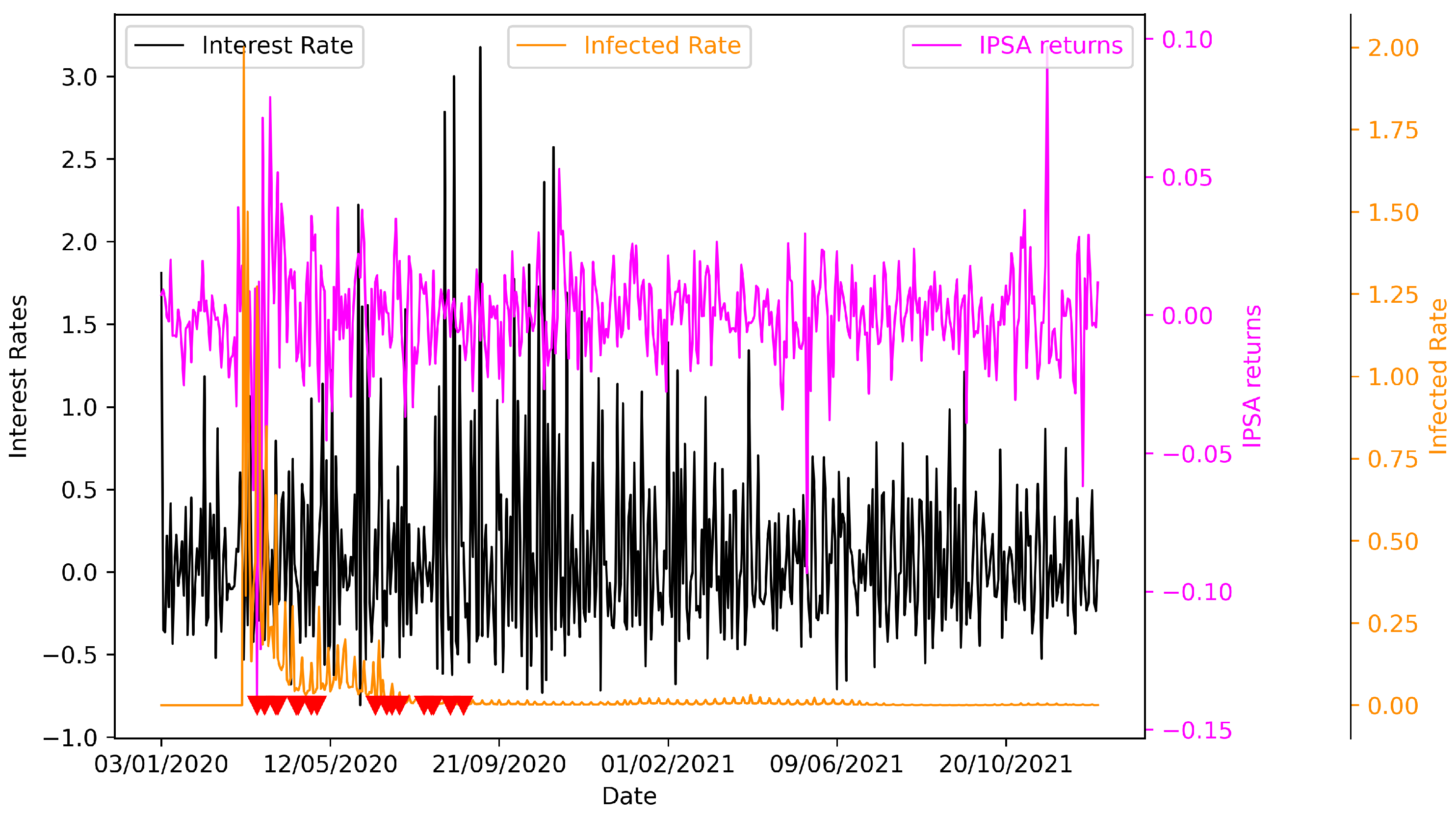
4.5. Chilean Case
5. Discussion
The Implications for the Involved Stakeholders
6. Conclusions
Author Contributions
Funding
Institutional Review Board Statement
Informed Consent Statement
Data Availability Statement
Conflicts of Interest
References
- World Bank. Global Economic Prospects, June 2020; World Bank: Washington, DC, USA, 2020; Available online: https://openknowledge.worldbank.org/handle/10986/33748 (accessed on 22 October 2023).
- Banco Central de Chile, Base de Datos Estadísticos, Cuentas Nacionales. Available online: https://si3.bcentral.cl/Siete/ES/Siete/Cuadro/CAP_CCNN/MN_CCNN76/CCNN2013_P2_MD/CCNN2013_P2_MD (accessed on 22 October 2023).
- Bloom, N.; Bunn, P.; Mizen, P.; Smietanka, P.; Thwaites, G. The Impact of COVID-19 on Productivity. Rev. Econ. Stat. 2023, 1–45. [Google Scholar] [CrossRef]
- Pak, A.; Adegboye, O.A.; Adekunle, A.I.; Rahman, K.M.; McBryde, E.S.; Eisen, D.P. Economic Consequences of the COVID-19 Outbreak: The Need for Epidemic Preparedness. Front. Public Health 2020, 8, 241. [Google Scholar] [CrossRef] [PubMed]
- Clemente-Suárez, V.J.; Navarro-Jiménez, E.; Jimenez, M.; Hormeño-Holgado, A.; Martinez-Gonzalez, M.B.; Benitez-Agudelo, J.C.; Perez-Palencia, N.; Laborde-Cárdenas, C.C.; Tornero-Aguilera, J.F. Impact of COVID-19 Pandemic in Public Mental Health: An Extensive Narrative Review. Sustainability 2021, 13, 3221. [Google Scholar] [CrossRef]
- Brzyska, J.; Szamrej-Baran, I. The COVID-19 Pandemic and the Implementation of Sustainable Development Goals: The EU Perspective. Sustainability 2023, 15, 13503. [Google Scholar] [CrossRef]
- Nicola, M.; Alsafi, Z.; Sohrabi, C.; Kerwan, A.; Al-Jabir, A.; Iosifidis, C.; Agha, M.; Agha, R. The socio-economic implications of the coronavirus pandemic (COVID-19): A review. Int. J. Surg. 2020, 78, 185–193. [Google Scholar] [CrossRef]
- Vasile, V.; Bunduchi, E. (Eds.) The Economic and Social Impact of the COVID-19 Pandemic; Springer: Cham, Switzerland, 2024. [Google Scholar]
- Ahmad, T.; Haroon, B.M.; Hui, J. Coronavirus Disease 2019 (COVID-19) Pandemic and Economic Impact. Pak. J. Med. Sci. 2020, 36, S73–S78. [Google Scholar] [CrossRef]
- Safonov, Y.; Borshch, V. Economic consequences of COVID-19 and the concepts of their overcoming. Ef. Ekon. 2020, 5. [Google Scholar] [CrossRef]
- Mofijur, M.; Fattah, I.R.; Alam, M.A.; Islam, A.S.; Ong, H.C.; Rahman, S.A.; Najafi, G.; Ahmed, S.F.; Uddin, M.A.; Mahlia, T.M.I. Impact of COVID-19 on the social, economic, environmental and energy domains: Lessons learnt from a global pandemic. Sustain. Prod. Consum. 2020, 26, 343–359. [Google Scholar] [CrossRef]
- Brodeur, A.; Gray, D.; Islam, A.; Bhuiyan, S. A literature review of the economics of COVID-19. J. Econ. Surv. 2021, 35, 1007–1044. [Google Scholar] [CrossRef]
- Mishra, N.P.; Das, S.S.; Yadav, S.; Khan, W.; Afzal, M.; Alarifi, A.; Kenawy, E.R.; Ansari, M.T.; Hasnain, M.S.; Nayak, A.K. Global impacts of pre- and post-COVID-19 pandemic: Focus on socio-economic consequences. Sens. Int. 2020, 1, 100042. [Google Scholar] [CrossRef] [PubMed]
- Simak, S.; Davydiuk, Y.; Burdeina, N.; Budiaiev, M.; Taran, O.; Ingram, K. Comprehensive assessment of the economic consequences of the COVID-19 pandemic. Sci. Bull. Natl. Min. Univ. 2020, 6, 168–173. [Google Scholar] [CrossRef]
- Barua, S. Understanding Coronanomics: The Economic Implications of the Coronavirus (COVID-19) Pandemic. 2020. Available online: https://papers.ssrn.com/sol3/papers.cfm?abstract_id=3566477 (accessed on 8 November 2023).
- Gavrilovic, K.; Vucekovic, M. Impact and Consequences of the COVID-19 Virus on the Economy of the United States. Int. Rev. 2020, 56–64. [Google Scholar] [CrossRef]
- Padhan, R.; Prabheesh, K.P. The Economics of COVID-19 Pandemic: A Survey. Econ. Anal. Pol. 2021, 70, 220–237. [Google Scholar] [CrossRef]
- Shcherbakov, G.A. The Impact and Consequences of the COVID-19 Pandemic: A Socio-Economic Dimension. WORLD (Mod. Innov. Dev.) 2021, 12, 8–22. [Google Scholar] [CrossRef]
- Rodela, T.T.; Tasnim, S.; Mazumder, H.; Faizah, F.; Sultana, A.; Hossain, M. Economic Impacts of Coronavirus Disease (COVID-19) in Developing Countries. 2020. Available online: https://osf.io/preprints/socarxiv/wygpk (accessed on 22 October 2023).
- Liu, W.-P.; Chu, Y.-C. FinTech, economic growth, and COVID-19: International evidence. Asia Pac. Manag. Rev. 2024, in press. [Google Scholar] [CrossRef]
- König, M.; Winkler, A. COVID-19: Lockdowns, Fatality Rates and GDP Growth. Intereconomics 2021, 56, 32–39. [Google Scholar] [CrossRef] [PubMed]
- Lassard Rosenthal, J.; Medina Núñez, C.; Palmero Picazo, J.; de la Parra Muñoz, B.E.; Mejía Martínez, L.L.; Rivas Morales, J.M. «SCORE-CoV-2» y su relación con el comportamiento del PIB. Anáhuac J. 2021, 21, 66–93. [Google Scholar] [CrossRef]
- Jena, P.R.; Majhi, R.; Kalli, R.; Managi, S.; Majhi, B. Impact of COVID-19 on GDP of major economies: Application of the artificial neural network forecaster. Econ. Anal. Policy 2021, 69, 324–339. [Google Scholar] [CrossRef]
- De la Fuente-Mella, H.; Rubilar, R.; Chahuán-Jiménez, K.; Leiva, V. Modeling COVID-19 Cases Statistically and Evaluating Their Effect on the Economy of Countries. Mathematics 2021, 9, 1558. [Google Scholar] [CrossRef]
- Ruiz-Estrada, M.A. COVID-19: Economic recession or depression? Estud. Econ. 2020, 37, 139–147. Available online: http://www.scielo.org.ar/scielo.php?script=sci_arttext&pid=S2525-12952020000200007&lng=es&tlng=en (accessed on 4 January 2023). [CrossRef]
- He, Y.; Zhang, Z. Energy and Economic Effects of the COVID-19 Pandemic: Evidence from OECD Countries. Sustainability 2022, 14, 12043. [Google Scholar] [CrossRef]
- Restrepo-Morales, J.A.; Valencia-Cárdenas, M.; García-Pérez-de-Lema, D. The role of technological innovation in the mitigation of the crisis generated by COVID-19: An empirical study of small and medium-sized businesses (SMEs) in Latin America. Int. Stud. Manag. Organ. 2024. [Google Scholar] [CrossRef]
- Wu, J. Cluster Analysis and k-Means Clustering: An Introduction in Advances in K-Means Clustering: A Data Mining Thinking; Springer Science & Business Media: New York, NY, USA, 2012; pp. 1–16. [Google Scholar]
- Benmahdi, M.; Lehsaini, M. Performance evaluation of main approaches for determining optimal number of clusters in wireless sensor networks. Int. J. Ad Hoc Ubiquitous Comput. 2020, 33, 184. [Google Scholar] [CrossRef]
- Halkidi, M. Hierarchial Clustering. In Encyclopedia of Database Systems; Liu, L., Özsu, M.T., Eds.; Springer: Boston, MA, USA, 2009. [Google Scholar] [CrossRef]
- Gohari, K.; Kazemnejad, A.; Sheidaei, A.; Hajari, S. Clustering of countries according to the COVID-19 incidence and mortality rates. BMC Public Health 2022, 22, 632. [Google Scholar] [CrossRef] [PubMed]
- Zarikas, V.; Poulopoulos, S.G.; Gareiou, Z.; Zervas, E. Clustering analysis of countries using the COVID-19 cases dataset. Data Brief 2020, 31, 105787. [Google Scholar] [CrossRef]
- Rizvi, S.A.; Umair, M.; Cheema, M.A. Clustering of countries for COVID-19 cases based on disease prevalence, health systems and environmental indicators. Chaos Solitons Fractals 2021, 151, 111240. [Google Scholar] [CrossRef]
- Sadeghi, B.; Cheung, R.C.Y.; Hanbury, M. Using hierarchical clustering analysis to evaluate COVID-19 pandemic preparedness and performance in 180 countries in 2020. BMJ Open 2021, 11, e049844. [Google Scholar] [CrossRef]
- Rahman, M.A.; Zaman, N.; Asyhari, A.T.; Al-Turjman, F.; Alam Bhuiyan, M.Z.; Zolkipli, M.F. Data-driven dynamic clustering framework for mitigating the adverse economic impact of COVID-19 lockdown practices. Sustain. Cities Soc. 2020, 62, 102372. [Google Scholar] [CrossRef]
- Sakoe, H.; Chiba, S. Dynamic programming algorithm optimization for spoken word recognition. IEEE Trans. Acoust. Speech Signal Process. 1978, 26, 43–49. [Google Scholar] [CrossRef]
- Yavuz, F.; Guney, Y.; Özdemir, Ş.; Tuaç, Y.; Arslan, O. The Clustering Structure of the COVID-19 Outbreak in Global Scale. Adv. Data Sci. Adapt. Anal. 2022, 14, 2250005. [Google Scholar] [CrossRef]
- Luo, Z.; Zhang, L.; Liu, N.; Wu, Y. Time series clustering of COVID-19 pandemic-related data. Data Sci. Manag. 2023, 6, 79–87. [Google Scholar] [CrossRef]
- Mahmoudi, M.; Baleanu, D.; Mansor, Z.; Tuan, B.; Kim-Hung, P. Fuzzy Clustering method to Compare the Spread Rate of Covid-19 in the High Risks Countries. Chaos Solitons Fractals 2020, 140, 110230. [Google Scholar] [CrossRef]
- Zhou, X.; Moinuddin, M. Impacts and implications of the COVID-19 crisis and its recovery for achieving sustainable development goals in Asia A review from an SDG interlinkage perspective. In Environmental Resilience and Transformation in Times of COVID-19; Elsevier: Amsterdam, The Netherlands, 2021; pp. 273–288. [Google Scholar] [CrossRef]
- Teresiené, D.; Keliuotyté-Staniuléniené, G.; Kanapickiené, R. Sustainable Economic Growth Support through Credit Transmission Channel and Financial Stability: In the Context of the COVID-19 Pandemic. Sustainability 2021, 13, 2692. [Google Scholar] [CrossRef]
- Przybytniowski, J.W.; Borkowski, S.; Grzebieniak, A.; Garasyim, P.; Dziekański, P.; Ciesielska, A. Social, Economic, and Financial Aspects of Modelling Sustainable Growth in the Irresponsible World during COVID-19 Pandemic. Sustainability 2022, 14, 12480. [Google Scholar] [CrossRef]
- World Bank Open Data | Total Population Using ID: WSP.POP.TOTL. Available online: https://data.worldbank.org/ (accessed on 22 October 2023).
- COVID-19 Finance Sector Related Policy Responses | Updated 18 January 2023. Available online: https://datacatalog.worldbank.org/search/dataset/0037999 (accessed on 22 October 2023).
- World Bank Open Data | GDP (Current US$). Available online: https://data.worldbank.org/indicator/NY.GDP.MKTP.CD (accessed on 22 October 2023).
- Feyen, E.; Gispert, T.A.; Kliatskova, T.; Mare, D.S. Financial Sector Policy Response to COVID-19 in Emerging Markets and Developing Economies. J. Bank. Financ. 2021, 133, 106184. [Google Scholar] [CrossRef]
- Chilean Stock Market Index IPSA Data from the Public Web Site. Available online: https://es.investing.com/indices/ipsa-historical-data (accessed on 22 October 2023).
- Annual Chilean Interest Rates Percentages, Monthly Base (TIP Colocaciones de 90 Días a un Año, no Reajustable). From Mean Rate of Financial System. Available online: https://si3.bcentral.cl/Indicadoressiete/secure/IndicadoresDiarios.aspx (accessed on 22 October 2023).
- Steinhaus, H. Sur la division des corps matériels en parties. Bull. L’AcadÉmie Pol. Des Sci. 1957, 4, 801–804. (In French) [Google Scholar]
- MacQueen, J. Some Methods for Classification and Analysis of Multivariate Observations. In Proceedings of the 5th Berkeley Symposium on Mathematical Statistics and Probability, Los Angeles, CA, USA, 21 June–18 July 1965; Volume 1, pp. 281–297. [Google Scholar]
- Nielsen, F. Hierarchical Clustering. In Introduction to HPC with MPI for Data Science. Undergraduate Topics in Computer Science; Springer: Cham, Switzerland, 2016. [Google Scholar] [CrossRef]
- Berndt, D.; Clifford, J. Using Dynamic Time Warping to Find Patterns in Time Series. In Proceedings of the 3rd International Conference on Knowledge Discovery and Data Mining, Seattle, WA, USA, 31 July–1 August 1994; AAAI Press: Washington, DC, USA, 1994; pp. 359–370. [Google Scholar]
- Li, H.; Liu, J.; Yang, Z.; Liu, R.W.; Wu, K.; Wan, Y. Adaptively constrained dynamic time warping for time series classification and clustering. Inf. Sci. 2020, 534, 97–116. [Google Scholar] [CrossRef]
- Thorndike, R.L. Who belongs in the family? Psychometrika 1953, 18, 267–276. [Google Scholar] [CrossRef]
- Rousseeuw, P.J. Silhouettes: A graphical aid to the interpretation and validation of cluster analysis. J. Comput. Appl. Math. 1987, 20, 53–65. [Google Scholar] [CrossRef]
- Tibshirani, R.; Guenther, W.; Hastie, T. Estimating the Number of Clusters in a Data Set via the Gap Statistic. J. R. Stat. Soc. Ser. B (Stat. Methodol.) 2001, 63, 411–423. [Google Scholar] [CrossRef]
- Brockwell, P.J.; Davis, R.A. (Eds.) Introduction to Time Series and Forecasting; Springer: New York, NY, USA, 2002. [Google Scholar] [CrossRef]
- Seabold, S.; Perktold, J. Statsmodels: Econometric and statistical modeling with python. In Proceedings of the 9th Python in Science Conference, Austin, TX, USA, 28 June–3 July 2010. [Google Scholar] [CrossRef]
- World Health Organization (WHO) Daily Cases and Deaths by Date Reported to WHO. Available online: https://covid19.who.int/WHO-COVID-19-global-data.csv (accessed on 22 October 2023).
- R Core Team. R: A Language and Environment for Statistical Computing; R Foundation for Statistical Computing: Vienna, Austria, 2023; Available online: https://www.R-project.org/ (accessed on 22 October 2023).
- FIAP. Retiro de Fondos: Desnaturalizando los Sistemas de Pensiones, una Mirada a los Efectos de Esta Politica Publica. 2021. Available online: www.fiapinternacional.org (accessed on 22 October 2023).
- Leal, D.; Jiménez, R.; Riquelme, M.; Leiva, V. Elliptical Capital Asset Pricing Models: Formulation, Diagnostics, Case Study with Chilean Data, and Economic Rationale. Mathematics 2023, 11, 1394. [Google Scholar] [CrossRef]
- Stehlik, M.; Leal, D.; Kiseak, J.; Leers, J.; Strelec, J.; Fuders, F. Stochastic approach to heterogeneity in short-time announcement effects on the Chilean stock market indexes within 2016–2019. Stoch. Anal. Appl. 2023, 42, 1–19. [Google Scholar] [CrossRef]
- Shuai, C.; Zhao, B.; Chen, X.; Liu, J.; Zheng, C.; Qu, S.; Zou, J.-P.; Xu, M. Quantifying the impacts of COVID-19 on Sustainable Development Goals using machine learning models. Fundam. Res. 2022. [Google Scholar] [CrossRef]
- Okuyama, Y.; Hewings, G.; Sonis, M. Sequential Interindustry Model (SIM) and Impact Analysis: Application for Measuring Economic Impact of Unscheduled Events. In Proceedings of the 47th North American Meetings of the Regional Science Association International, Chicago, IL, USA, 9–11 November 2000. [Google Scholar]


| OECD Member (with Ratification Date) | Not OECD Member |
|---|---|
| Australia—7 June 1971 | Argentina |
| Austria—29 September 1961 | Bolivia |
| Belgium—13 September 1961 | Brazil |
| Canada—10 April 1961 | Bulgaria |
| Chile—7 May 2010 | China |
| Colombia—28 April 2020 | Ecuador |
| Costa Rica—25 May 2021 | India |
| Czechia —21 December 1995 | Indonesia |
| Denmark—30 May 1961 | Paraguay |
| Estonia—9 December 2010 | Perú |
| Finland—28 January 1969 | Romania |
| France—7 August 1961 | Russia |
| Germany—27 September 1961 | South Africa |
| Greece—27 September 1961 | Uruguay |
| Hungary—7 May 1996 | |
| Iceland—5 June 1961 | |
| Ireland—17 August 1961 | |
| Israel—7 September 2010 | |
| Italy—29 March 1962 | |
| Japan—28 April 1964 | |
| Latvia—1 July 2016 | |
| Lithuania—5 July 2018 | |
| Luxemburg—7 December 1961 | |
| Mexico—18 May 1994 | |
| Netherlands—13 November 1961 | |
| New Zealand—29 May 1973 | |
| Norway—4 July 1961 | |
| Poland—22 November 1996 | |
| Portugal—4 August 1961 | |
| Slovakia—14 December 2000 | |
| Slovenia—21 July 2010 | |
| South Korea—12 December 1996 | |
| Spain—3 August 1961 | |
| Sweden—28 September 1961 | |
| Switzerland—28 September 1961 | |
| Turkiye—2 August 1961 | |
| United Kingdom—2 May 1961 | |
| United States—12 April 1961 |
| Variable | N | Mean | Std. Dev. | Min | Pctl. 25 | Pctl. 75 | Max |
|---|---|---|---|---|---|---|---|
| Measures | 52 | 46.096 | 39.825 | 0 | 0.000 | 79.000 | 134 |
| Infected | 52 | 10,568.8 | 5894.7 | 9.3 | 6539.3 | 14,700.5 | 23,961.3 |
| 52 | −0.0416 | 0.0618 | −0.212 | −0.0822 | 0.00613 | 0.0664 | |
| 52 | 0.0995 | 0.0801 | −0.119 | 0.0529 | 0.142 | 0.263 |
| Variable | Ctr1 | Ctr2 | ||
|---|---|---|---|---|
| GDP 19–20 | 42.88 | 0.0848 | 0.8323 | 0.0009 |
| GDP 19–21 | 40.43 | 0.0001 | 0.7849 | 0.0000 |
| Infected | 12.78 | 27.22 | 0.2481 | 0.2773 |
| Measures | 3.89 | 72.70 | 0.0755 | 0.7408 |
| Measures | Cluster 1 | Cluster 2 |
|---|---|---|
| Banking sector | 0.53852 | 0.61874 |
| Financial Markets/NBFIs | 0.15871 | 0.16197 |
| Insolvency | 0.01926 | 0.01456 |
| Liquidity/Funding | 0.24576 | 0.19654 |
| Payment Systems | 0.03775 | 0.00819 |
| Date | Level 1 Policy Measures | Level 2 Policy Measures |
|---|---|---|
| 16 March 2020 | Liquidity/Funding | Asset purchases |
| 16 March 2020 | Liquidity/Funding | Liquidity (incl FX)/ELA |
| 20 March 2020 | Liquidity/Funding | Liquidity (incl FX)/ELA |
| 16 March 2020 | Liquidity/Funding | Liquidity (incl FX)/ELA |
| 16 March 2020 | Liquidity/Funding | Policy rate |
| 16 March 2020 | Banking Sector | Support borrowers |
| 30 March 2020 | Banking Sector | Operational continuity |
| 31 March 2020 | Liquidity/Funding | Policy rate |
| 15 April 2020 | Financial Markets/NBFIs | NBFIs |
| 27 April 2020 | Banking Sector | Prudential |
| 30 April 2020 | Banking Sector | Support borrowers |
| 30 April 2020 | Banking Sector | Support borrowers |
| 16 April 2020 | Banking Sector | Support borrowers |
| 16 June 2020 | Liquidity/Funding | Liquidity (incl FX)/ELA |
| 24 June 2020 | Liquidity/Funding | Liquidity (incl FX)/ELA |
| 29 June 2020 | Banking Sector | Support borrowers |
| 05 July 2020 | Banking Sector | Support borrowers |
| 05 July 2020 | Banking Sector | Support borrowers |
| 05 July 2020 | Banking Sector | Support borrowers |
| 24 July 2020 | Liquidity/Funding | Liquidity (incl FX)/ELA |
| 24 July 2020 | Financial Markets/NBFIs | NBFIs |
| 30 July 2020 | Liquidity/Funding | Liquidity (incl FX)/ELA |
| 30 July 2020 | Liquidity/Funding | Asset purchases |
| 30 July 2020 | Liquidity/Funding | Liquidity (incl FX)/ELA |
| 31 July 2020 | Banking Sector | Prudential |
| 13 August 2020 | Liquidity/Funding | Asset purchases |
| 24 August 2020 | Banking Sector | Prudential |
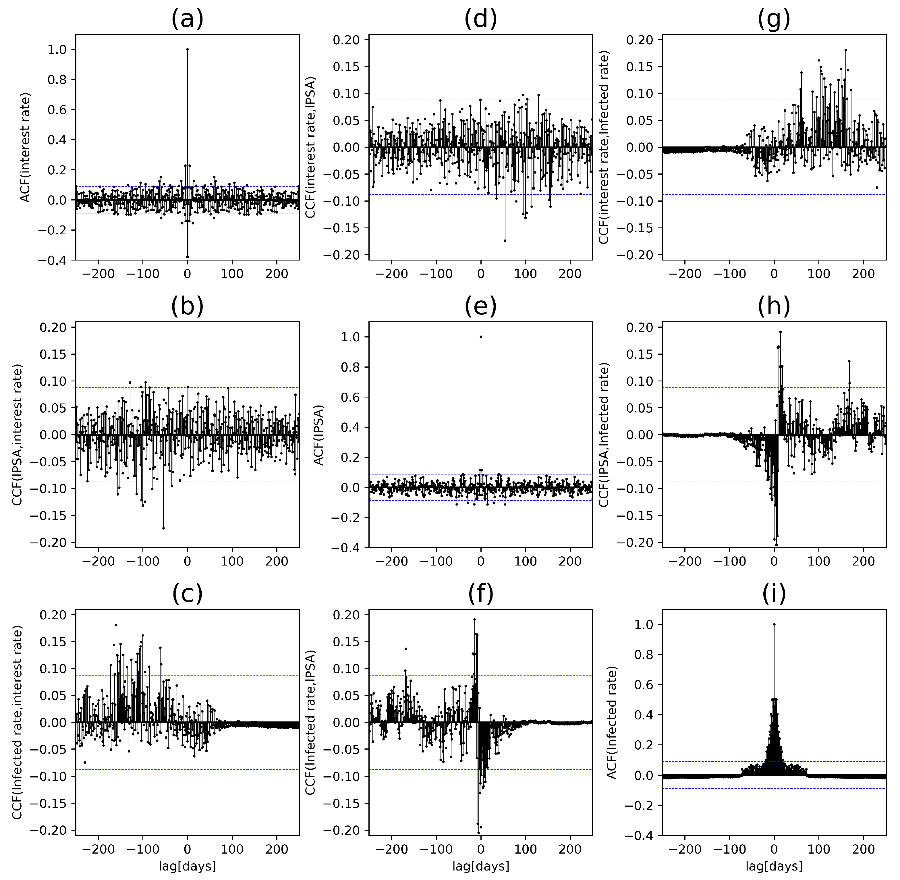
| Function (CCF or ACF) | lag | max (CCF) or max (ACF) |
|---|---|---|
| ACF (Interest rate) | 1 | −0.37925 |
| CCF (Interest rate, IPSA) | 54 | −0.17408 |
| CCF (Interest rate, Infected rate) | 160 | 0.18057 |
| CCF (IPSA, Interest rate) | −54 | −0.17408 |
| ACF (IPSA) | 2 | 0.11375 |
| CCF (IPSA, Infected rate) | 5 | −0.20480 |
| CCF (Infected rate, Interest rate) | −160 | 0.18057 |
| CCF (Infected rate, IPSA) | −5 | −0.20480 |
| ACF (Infected rate) | 2 | 0.50206 |
Disclaimer/Publisher’s Note: The statements, opinions and data contained in all publications are solely those of the individual author(s) and contributor(s) and not of MDPI and/or the editor(s). MDPI and/or the editor(s) disclaim responsibility for any injury to people or property resulting from any ideas, methods, instructions or products referred to in the content. |
© 2024 by the authors. Licensee MDPI, Basel, Switzerland. This article is an open access article distributed under the terms and conditions of the Creative Commons Attribution (CC BY) license (https://creativecommons.org/licenses/by/4.0/).
Share and Cite
Nicolis, O.; Maidana, J.P.; Contreras, F.; Leal, D. Analyzing the Impact of COVID-19 on Economic Sustainability: A Clustering Approach. Sustainability 2024, 16, 1525. https://doi.org/10.3390/su16041525
Nicolis O, Maidana JP, Contreras F, Leal D. Analyzing the Impact of COVID-19 on Economic Sustainability: A Clustering Approach. Sustainability. 2024; 16(4):1525. https://doi.org/10.3390/su16041525
Chicago/Turabian StyleNicolis, Orietta, Jean Paul Maidana, Fabian Contreras, and Danilo Leal. 2024. "Analyzing the Impact of COVID-19 on Economic Sustainability: A Clustering Approach" Sustainability 16, no. 4: 1525. https://doi.org/10.3390/su16041525
APA StyleNicolis, O., Maidana, J. P., Contreras, F., & Leal, D. (2024). Analyzing the Impact of COVID-19 on Economic Sustainability: A Clustering Approach. Sustainability, 16(4), 1525. https://doi.org/10.3390/su16041525