
Nuʻupia Ponds’ Water Circulation Characteristics: Exploring Water Exchange and Residence Time for Marine Ecosystem Management


Abstract
1. Introduction
2. Methods
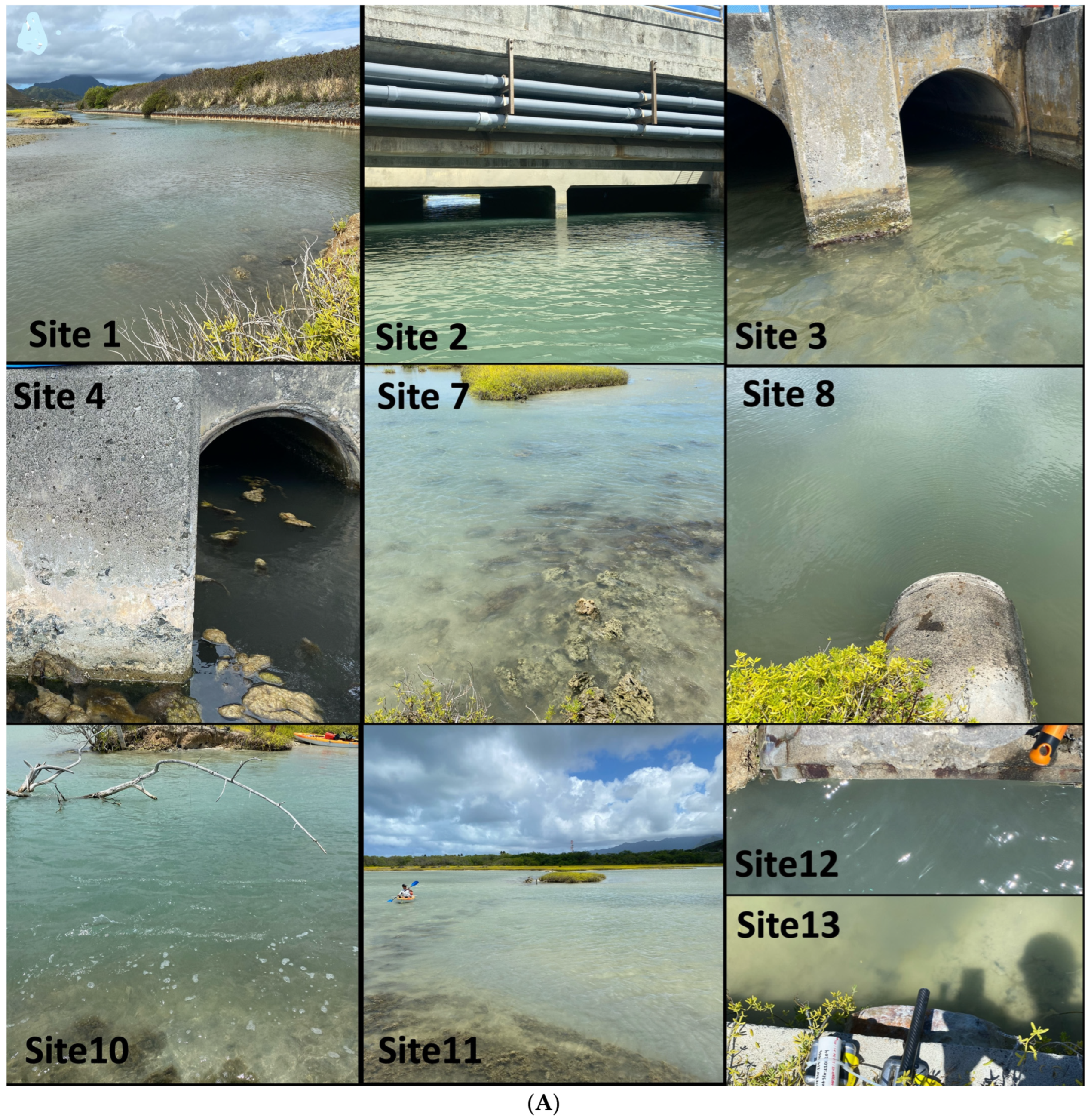
2.1. Nuʻupia Ponds Study Site
2.2. Water Volume Flux and Volume Change Calculations
2.3. Pond Bathymetries, Volumes, and Residence Times
3. Results
3.1. Characterization of Meteorological Conditions
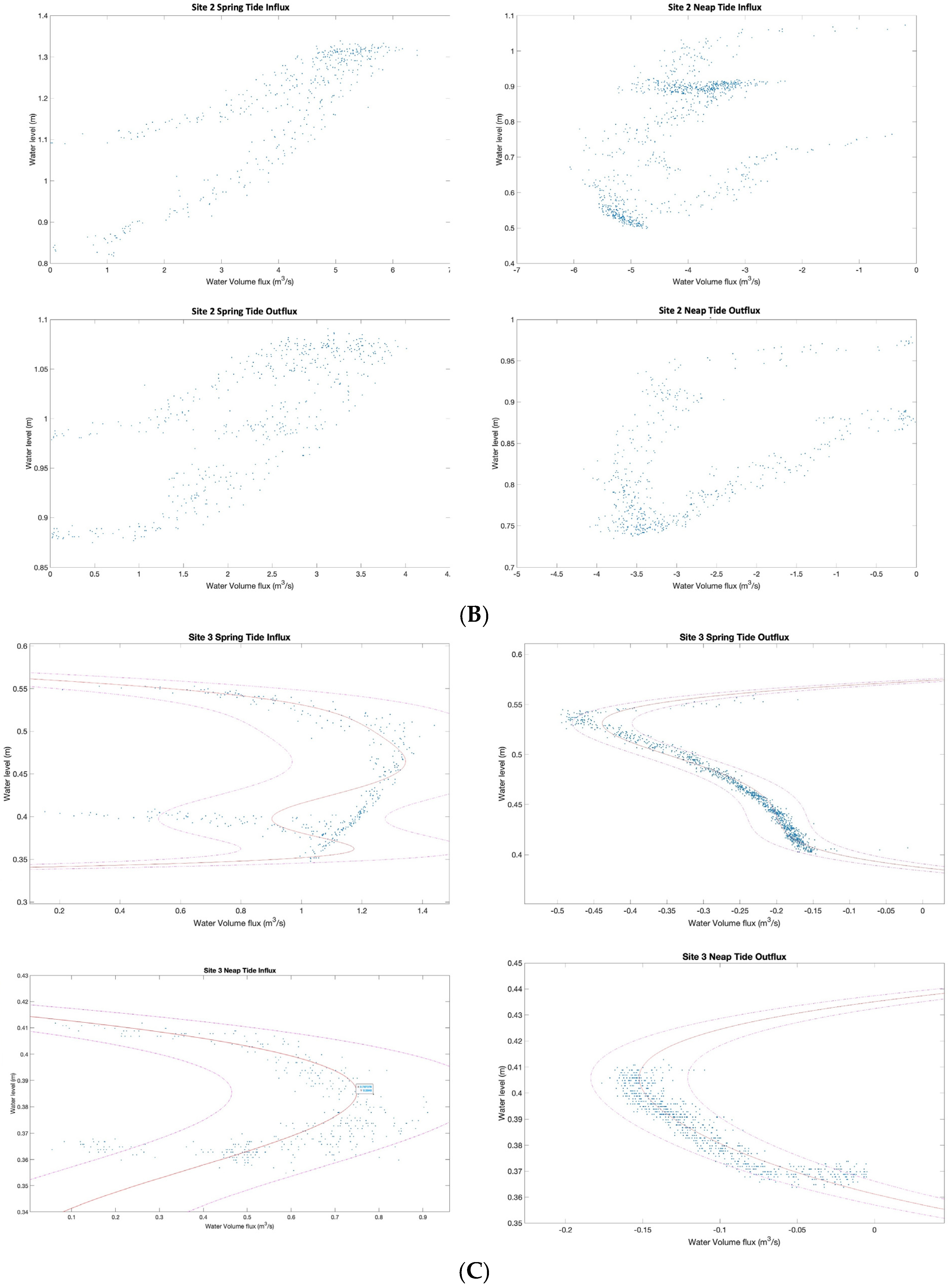
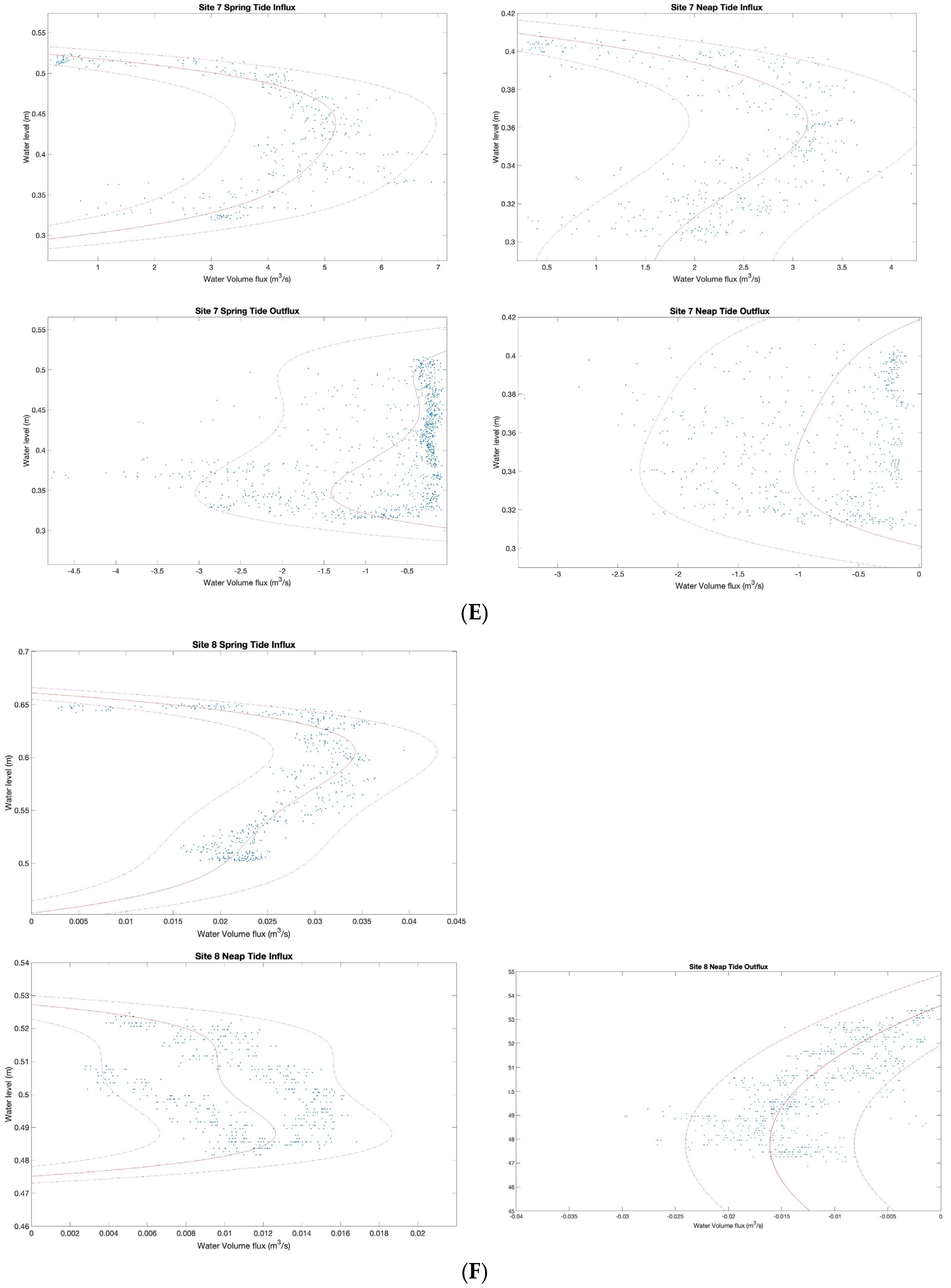
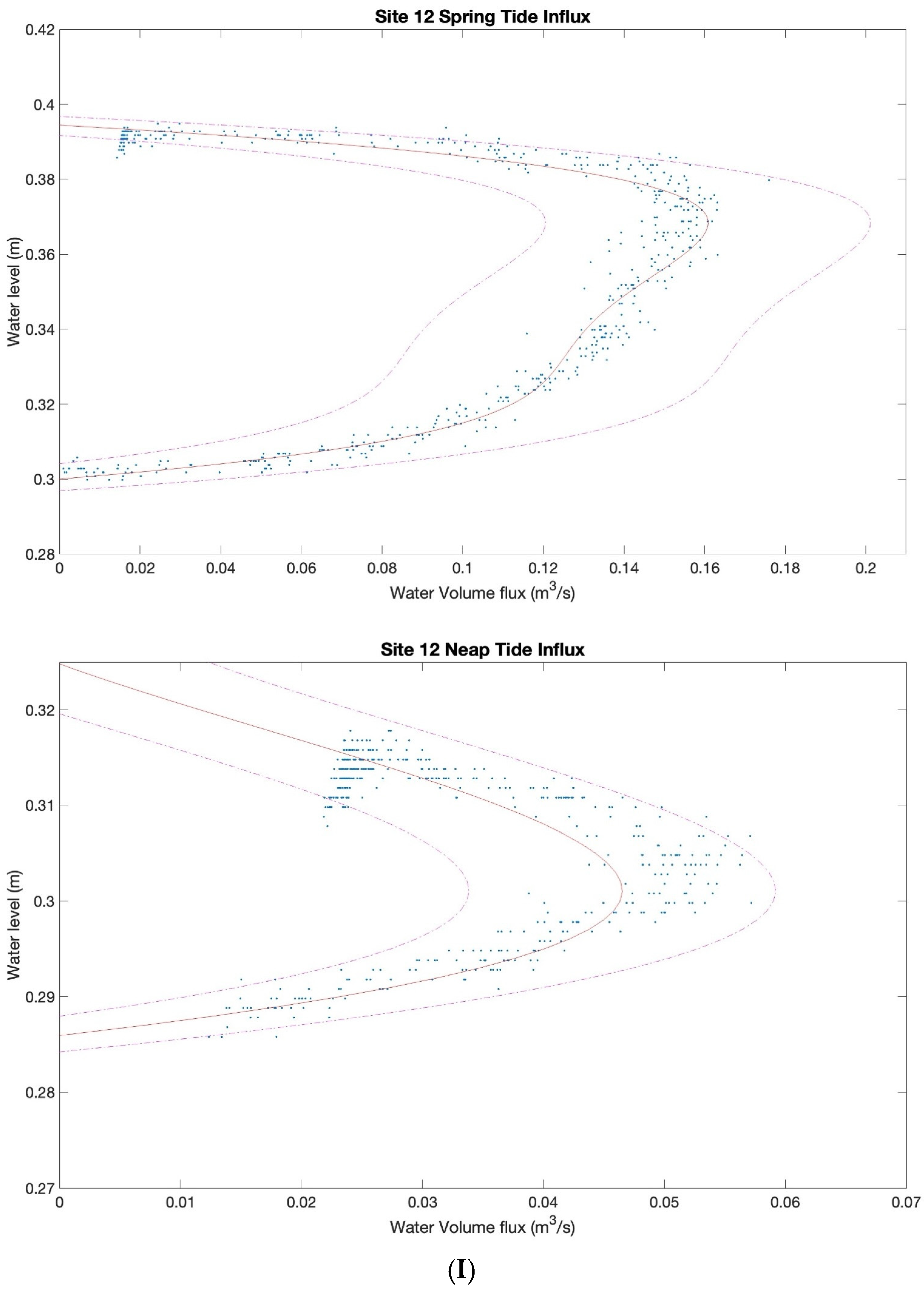
3.2. Characterizing Water Volume Flux
3.3. Water Flux Lags across Nuʻupia Ponds System
3.4. Nuʻupia Volumes, Exchange Rates, and Residence Times
4. Discussion
4.1. Site Specific Details and Technical Limitations
4.2. Management Implications
Author Contributions
Funding
Data Availability Statement
Acknowledgments
Conflicts of Interest
Appendix A


References
- Safak, I.; Wiberg, P.L.; Richardson, D.L.; Kurum, M.O. Controls on residence time and exchange in a system of shallow coastal bays. Cont. Shelf Res. 2015, 97, 7–20. [Google Scholar]
- Kim, C.-K.; Park, K.; Powers, S.P.; Graham, W.M.; Bayha, K.M. Oyster Larval Transport in Coastal Alabama: Dominance of Physical Transport over Biological Behavior in a Shallow Estuary. J. Geophys. Res. Oceans 2010, 115, C10019. [Google Scholar]
- Defne, Z.; Ganju, N.K. Quantifying the Residence Time and Flushing Characteristics of a Shallow, Back-Barrier Estuary: Application of Hydrodynamic and Particle Tracking Models. Estuaries Coasts 2015, 38, 1719–1734. [Google Scholar]
- Möhlenkamp, P.; Beebe, C.K.; McManus, M.A.; Kawelo, A.H.; Kotubetey, K.; Lopez-Guzman, M.; Nelson, C.E.; Alegado, R. Kū Hou Kuapā: Cultural Restoration Improves Water Budget and Water Quality Dynamics in Heʻeia Fishpond. Sustainability 2019, 11, 161. [Google Scholar]
- Keala, G.; Hollyer, J.R.; Castro, L. Loko Ia: A Manual on Hawaiian Fishpond Restoration and Management; University of Hawaiʻi at Manoa: Honolulu, HI, USA, 2007. [Google Scholar]
- Wyban, C.A. Tide and Current: Fishponds of Hawaii; University of Hawaiʻi Press: Honolulu, HI, USA, 2020. [Google Scholar]
- Cornwell, E. Island Empowerment as Global Endowment: Understanding Hawaiian Adaptive Cultural Resource Management. J. Undergrad. Ethnogr. 2020, 10, 69–90. [Google Scholar]
- Cobb, J.N. The Commercial Fisheries of the Hawaiian Islands in 1903; U.S. Government Printing Office: Washington, DC, USA, 1905.
- Marine Corps Base Hawaiʻi. Nuʻupia Ponds: Heart of Mokapu Watershed; Marine Corps Base Hawaiʻi: Honolulu, HI, USA, 1998; 10. [Google Scholar]
- Malama Aina O Mokapu: Protecting Mokapu Lands; U.H. Sea Grant College Program, University of Hawaiʻi, Manoa: Honolulu, HI, USA, 1992.
- Marine Corps Base Hawaiʻi. Assessment for Nuʻupia Ponds Habitat Improvement Projects at Nuʻupia Wildlife Management Area; Marine Corps Base Hawaiʻi: Honolulu, HI, USA, 1996. [Google Scholar]
- Board of Commissioners of Agriculture and Forestry. Report of the Board of Commissioners of Agriculture and Forestry of the Territory of Hawaii for the Period…; Board of Commissioners of Agriculture and Forestry: Honolulu, HI, USA, 1908.
- Chimner, R.A.; Fry, B.; Kaneshiro, M.Y.; Cormier, N. Current Extent and Historical Expansion of Introduced Mangroves on Oahu, Hawaiʻi. Pac. Sci. 2006, 60, 377–383. [Google Scholar]
- Cox, E.; Allen, J. Stand Structure and Productivity of the Introduced Rhizophora Mangle in Hawaii. Estuaries 1999, 22, 276–284. [Google Scholar]
- Universal User Guide for TCM-x Current Meters, MAT-1 Data Logger and Domino Software; Lowell Instruments: East Famouth, MA, USA, 2022.
- McCoy, D.; McManus, M.A.; Kotubetey, K.; Kawelo, A.H.; Young, C.; D’Andrea, B.; Ruttenberg, K.C.; Alegado, R.‘A. Large-Scale Climatic Effects on Traditional Hawaiian Fishpond Aquaculture. PLoS ONE 2017, 12, e0187951. [Google Scholar]
- Young, C.W. Perturbation of Nutrient Level Inventories and Phytoplankton Community Composition During Storm Events in a Tropical Coastal System: Heeia Fishpond, Oahu, Hawaii. Master’s Thesis, University of Hawaiʻi Manoa, Honolulu, HI, USA, 2011. [Google Scholar]
- Li, Y.; Xiong, X.; Zhang, C.; Liu, A. Sustainable Restoration of Anoxic Freshwater Using Environmentally-Compatible Oxygen-Carrying Biochar: Performance and Mechanisms. Water Res. 2022, 214, 118204. [Google Scholar]
- Baxa, M.; Musil, M.; Kummel, M.; Hanzlík, P.; Tesařová, B.; Pechar, L. Dissolved Oxygen Deficits in a Shallow Eutrophic Aquatic Ecosystem (Fishpond)—Sediment Oxygen Demand and Water Column Respiration Alternately Drive the Oxygen Regime. Sci. Total Environ. 2021, 766, 142647. [Google Scholar]
- Breitburg, D.; Levin, L.A.; Oschlies, A.; Grégoire, M.; Chavez, F.P.; Conley, D.J.; Garçon, V.; Gilbert, D.; Gutiérrez, D.; Isensee, K.; et al. Declining oxygen in the global ocean and coastal waters. Science 2018, 359, eaam7240. [Google Scholar] [PubMed]
- Gedan, K.; Kirwan, M.; Wolanski, E.; Barbier, E.; Silliman, B. The Present and Future Role of Coastal Wetland Vegetation in Protecting Shorelines: Answering Recent Challenges to the Paradigm. Clim. Change 2010, 106, 7–29. [Google Scholar]
- Twilley, R.; Lugo, A.; Patterson-Zucca, C. Litter Production and Turnover in Basin Mangrove Forests in Southwest Florida. Ecology 1986, 67, 670–683. [Google Scholar]
- Allen, J.A. Mangroves as Alien Species: The Case of Hawaii. Glob. Ecol. Biogeogr. Lett. 1998, 7, 61–71. [Google Scholar]
- Drigot, D.C. Mangrove Removal and Related Studies at Marine Corps Base Hawaii. Tech Note M-3N in Technical Notes: Case Studies from the Department of Defense Conservation Program; U.S. Dept. of Defense Legacy Resource Management Program Publication: Honolulu, HI, USA, 1999; pp. 170–174. [Google Scholar]
- Walsh, G.E. An Ecological Study of a Hawaiian Mangrove Swamp. Estuaries 1967, 83, 420–431. [Google Scholar]
- Crooks, J.A. Characterizing Ecosystem-Level Consequences of Biological Invasions: The Role of Ecosystem Engineers. Oikos 2002, 97, 153–166. [Google Scholar]
- Rauzon, M.J.; Drigot, D.C. Red Mangrove Eradication and Pickleweed Control in a Hawaiian Wetland, Waterbird Responses, and Lessons Learned. In Turning the Tide: The Eradication of Invasive Species; Veitch, C.R., Clout, M.N., Eds.; IUCN SSC Invasive Species Specialist Group, IUCN: Gland, Switzerland; Cambridge, UK, 2002; pp. 240–248. [Google Scholar]
- Drigot, D.C. An Ecosystem-Based Management Approach to Enhancing Endangered Waterbird Habitat on a Military Base. Stud. Avian Biol. 2001, 22, 329–337. [Google Scholar]
- Gautreau, E.; Volatier, L.; Nogaro, G.; Gouze, E.; Mermillod-Blondin, F. The Influence of Bioturbation and Water Column Oxygenation on Nutrient Recycling in Reservoir Sediments. Hydrobiologia 2020, 847, 1027–1040. [Google Scholar]
- Karlson, K.; Rosenberg, R.; Bonsdorff, E. Temporal and Spatial Large-Scale Effects of Eutrophication and Oxygen Deficiency on Benthic Fauna in Scandinavian and Baltic Waters—A Review. Oceanogr. Mar. Biol. 2002, 40, 427–489. [Google Scholar]
- Roberts, D.A. Causes and Ecological Effects of Resuspended Contaminated Sediments (RCS) in Marine Environments. Environ. Int. 2012, 40, 230–243. [Google Scholar]
- Wenger, A.S.; Harvey, E.; Wilson, S.; Rawson, C.; Newman, S.J.; Clarke, D.; Saunders, B.J.; Browne, N.; Travers, M.J.; McIlwain, J.L.; et al. A critical analysis of the direct effects of dredging on fish. Fish Fish. 2017, 18, 967–98533. [Google Scholar]
- Thrush, S.F.; Dayton, P.K. Disturbance to Marine Benthic Habitats by Trawling and Dredging: Implications for Marine Biodiversity. Annu. Rev. Ecol. Evol. Syst. 2002, 33, 449–473. [Google Scholar]


| Exchange Point | Ponds Connected | Latitude | Longitude | Heading | Total Width (m) | Instrument | Description |
|---|---|---|---|---|---|---|---|
| Site 1 | Channel and Halekou | 21.43745 | −157.753614 | 90°/270° | 39 | CM, PS | 3 Gaps |
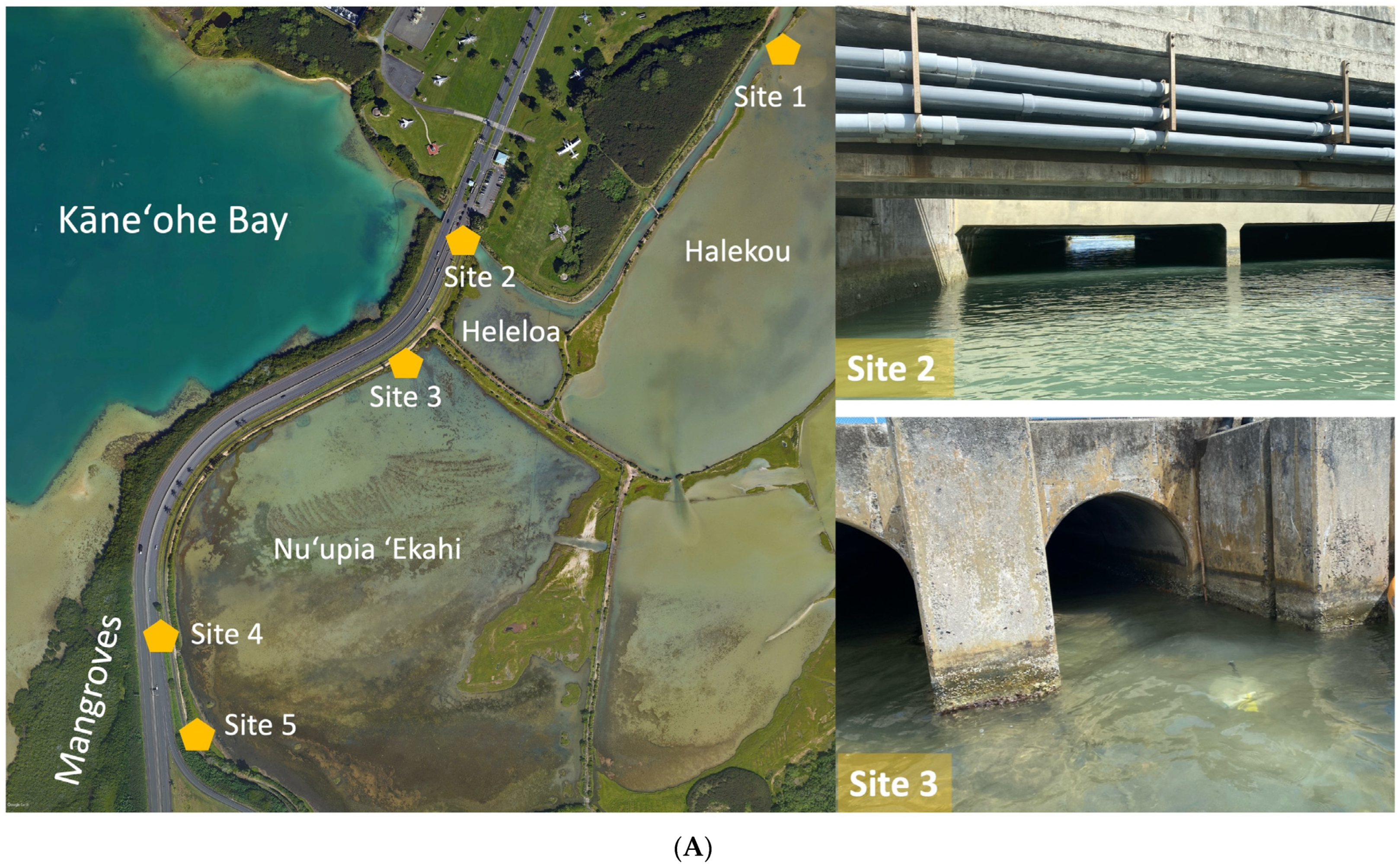
| Site 2 | Kāneʻohe Bay and Channel/Heleloa | 21.43527 | −157.756953 | 121°/318° | 11 | CM, PS | Bridge |
| Site 3 | Kāneʻohe Bay and Nuʻupia ʻEkahi | 21.43404 | −157.757554 | 125°/305° | 3.45 | CM, PS | 3 Culverts |
| Site 4 | Kāneʻohe Bay and Nuʻupia ʻEkahi | 21.43086 | −157.760024 | 82°/na | 2.2 | CM, PS | 2 Culverts |
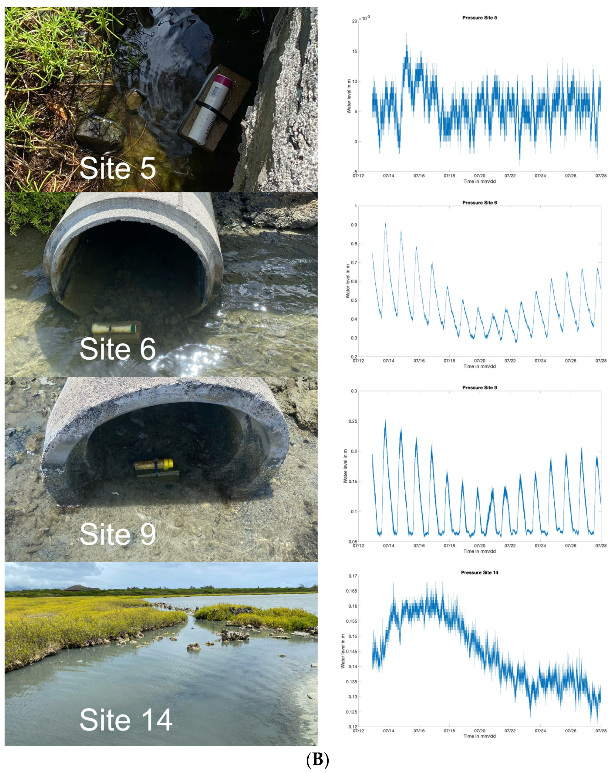
| Site 5 | NA | 21.42960 | −157.75913 | na/na | na | PS | 1 Culvert |
| Site 6 | Nuʻupia ʻEkahi and Nuʻupia ʻElua | 21.42948 | −157.755293 | na/na | 1.4 | PS | 2 Culverts |
| Site 7 | Nuʻupia ʻElua and Nuʻupia ʻEkolu | 21.43208 | −157.752659 | 80°/260° | 68 | CM, PS | 3 Gaps |
| Site 8 | Nuʻupia ʻEkahi and Nuʻupia ʻElua | 21.43214 | −157.755238 | 80°/285° | 0.75 | CM, PS | 1 Culvert |
| Site 9 | Nuʻupia ʻEkahi and Halekou | 21.43298 | −157.755018 | na/na | 0.85 | PS | 1 Culvert |
| Site 10 | Halekou and Nuʻupia ʻElua | 21.43284 | −157.754489 | 150°/345° | 10 | CM, PS | 1 Gap |
| Site 11 | Halekou and Nuʻupia ʻEkolu | 21.43486 | −157.751989 | 130°/303° | 12 | CM, PS | 1 Gap |
| Site 12 | Nuʻupia ʻEkolu and Nuʻupia ʻEhā | 21.43123 | −157.743009 | 91°/na | 1.2 | CM, PS | 2 Culverts |
| Site 13 | Nuʻupia ʻEhā and Kaluapuhi | 21.43116 | −157.742126 | 82°/230° | 0.8 | CM, PS | 2 Culverts |
| Site 14 | Kaluapuhi and Paʻakai | 21.43275 | −157.739312 | na/na | 3 | PS | 1 Gap |
| Mean WVF (m3 s−1) | Peak WVF (m3 s−1) | Average vx (m s−1) | Tidal Cycle Length (h) | WVF Rate (m3 h−1) | Volume Exchanged per Tidal Cycle (m3) | Relative WVF (%) | |
|---|---|---|---|---|---|---|---|
| Spring Influx | |||||||
| Site 1 | 6.97 | 10.74 | 0.33 | 6.17 | 25,082 | 154,753 | 30.1 |
| Site 2 | 4.01 | 6.43 | 0.30 | 7.62 | 14,437 | 110,011 | 21.4 |
| Site 3 | 1.02 | 1.44 | 0.68 | 6.5 | 3667 | 23,835 | 4.6 |
| Site 4 | 0.39 | 0.56 | 0.35 | 5.01 | 1411 | 7070 | 1.4 |
| Site 5 | 0.00 | 0.00 | 0.00 | 0 | 0 | 0 | 0 |
| Site 6 | na | na | na | na | na | na | <1 |
| Site 7 | 3.69 | 7.10 | 0.13 | 7.1 | 13,273 | 94,237 | 18.3 |
| Site 8 | 0.03 | 0.04 | 0.06 | 8.73 | 91 | 798 | 0.2 |
| Site 9 | na | na | na | na | na | na | <1 |
| Site 10 | 2.39 | 3.49 | 0.34 | 6.9 | 8599 | 59,333 | 11.5 |
| Site 11 | 2.18 | 3.06 | 0.41 | 7.68 | 7863 | 60,392 | 11.7 |
| Site 12 | 0.09 | 0.18 | 0.22 | 9.16 | 337 | 3083 | 0.6 |
| Site 13 | 0.02 | 0.03 | 0.08 | 10.89 | 65 | 710 | 0.1 |
| Site 14 | na | na | na | na | na | na | <1 |
| Spring Outflux | |||||||
| Site 1 | −2.87 | −5.07 | 0.18 | 16.68 | −10,333 | −172,362 | 25.7 |
| Site 2 | −4.18 | −6.07 | 0.54 | 16.72 | −15,033 | −251,350 | 37.5 |
| Site 3 | −0.26 | −0.50 | 0.16 | 17.96 | −942 | −16,920 | 2.5 |
| Site 4 | no outflux | no outflux | no outflux | no outflux | no outflux | no outflux | 0 |
| Site 5 | 0.00 | 0.00 | 0.00 | 0 | 0 | 0 | 0 |
| Site 6 | na | na | na | na | na | na | <1 |
| Site 7 | −0.81 | −4.77 | 0.03 | 17.55 | −2921 | −51,271 | 7.6 |
| Site 8 | no outflux | no outflux | no outflux | no outflux | no outflux | no outflux | 0 |
| Site 9 | na | na | na | na | na | na | <1 |
| Site 10 | −1.51 | −2.49 | 0.23 | 16.96 | −5454 | −92,494 | 13.8 |
| Site 11 | −1.45 | −2.07 | 0.30 | 16.22 | −5233 | −84,884 | 12.7 |
| Site 12 | no outflux | no outflux | no outflux | no outflux | no outflux | no outflux | 0 |
| Site 13 | −0.03 | −0.04 | 0.18 | 10.13 | −114 | −1160 | 0.2 |
| Site 14 | na | na | na | na | na | na | <1 |
| Neap Influx | |||||||
| Site 1 | 3.10 | 5.55 | 0.17 | 8.28 | 11,156 | 92,369 | 27.7 |
| Site 2 | 2.28 | 4.01 | 0.20 | 8.71 | 8195 | 71,382 | 21.4 |
| Site 3 | 0.56 | 0.91 | 0.43 | 6.88 | 2030 | 13,967 | 4.2 |
| Site 4 | 0.01 | 0.01 | 0.01 | 12.53 | 19 | 244 | 0.1 |
| Site 5 | na | na | na | na | na | na | 0 |
| Site 6 | na | na | na | na | na | na | <1 |
| Site 7 | 2.28 | 4.20 | 0.10 | 8.12 | 8215 | 66,705 | 20.0 |
| Site 8 | 0.05 | 0.11 | 0.12 | 12.4 | 165 | 2049 | 0.6 |
| Site 9 | na | na | na | na | na | na | <1 |
| Site 10 | 1.77 | 2.55 | 0.26 | 8.03 | 6363 | 51,098 | 15.3 |
| Site 11 | 0.93 | 1.61 | 0.20 | 10.38 | 3342 | 34,692 | 10.4 |
| Site 12 | 0.03 | 0.06 | 0.09 | 7.48 | 118 | 886 | 0.3 |
| Site 13 | no influx | no influx | no influx | no influx | no influx | no influx | 0 |
| Site 14 | na | na | na | na | na | na | <1 |
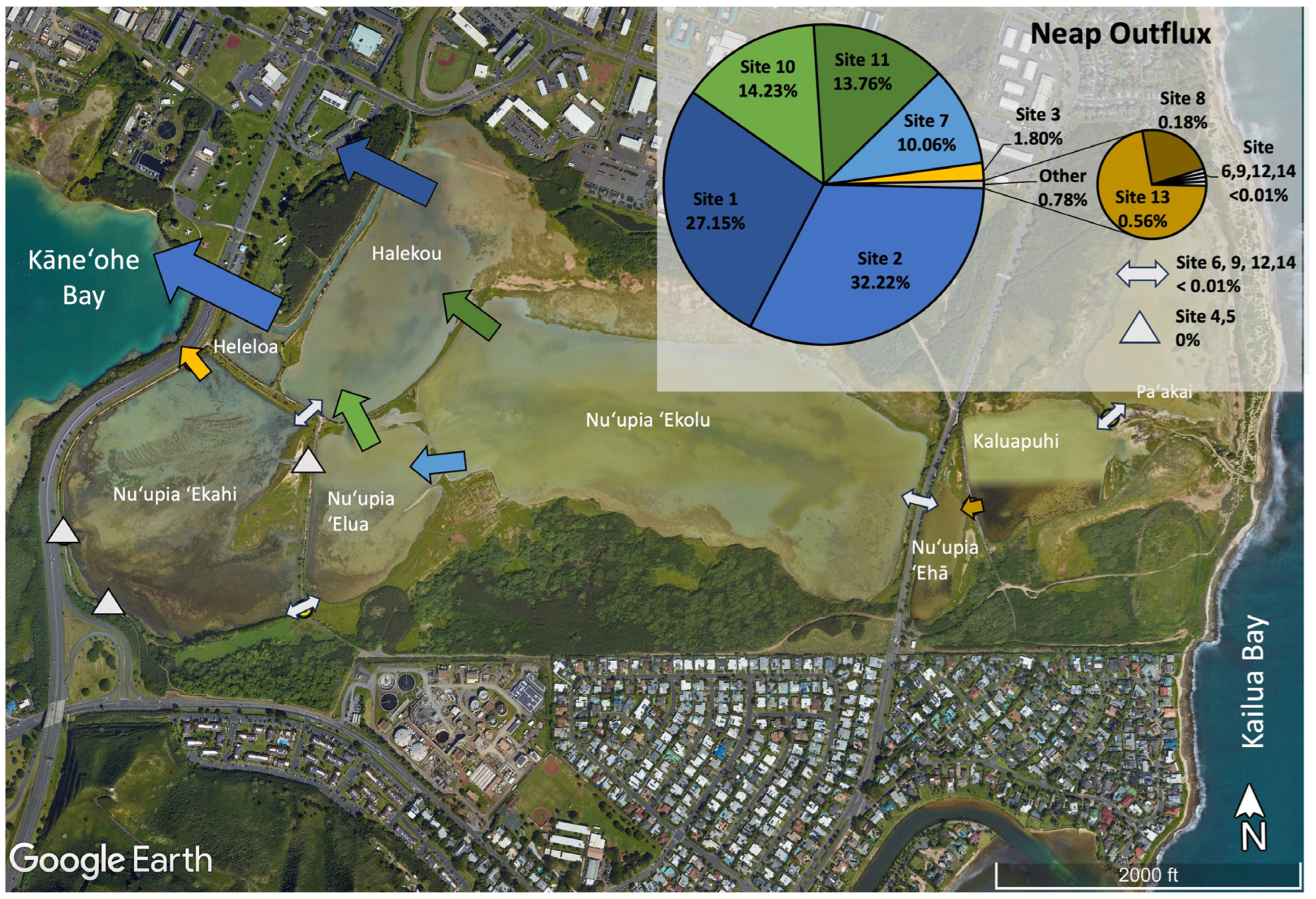
| Neap Outflux | |||||||
| Site 1 | −2.94 | −1.60 | 0.19 | 7.5 | −10,570 | −79,275 | 27.2 |
| Site 2 | −2.76 | −4.16 | 0.31 | 9.48 | −9924 | −94,077 | 32.2 |
| Site 3 | −0.11 | −0.18 | 0.08 | 13.55 | −388 | −5254 | 1.8 |
| Site 4 | no outflux | no outflux | no outflux | no outflux | no outflux | no outflux | 0 |
| Site 5 | na | na | na | na | na | na | 0 |
| Site 6 | na | na | na | na | na | na | <1 |
| Site 7 | −0.83 | −3.28 | 0.04 | 9.83 | −2989 | −29,386 | 10.1 |
| Site 8 | −0.01 | −0.03 | 0.03 | 11.93 | −44 | −524 | 0.2 |
| Site 9 | na | na | na | na | na | na | <1 |
| Site 10 | −1.29 | −2.12 | 0.20 | 8.96 | −4637 | −41,549 | 14.2 |
| Site 11 | −1.18 | −1.68 | 0.26 | 9.5 | −4230 | −40,188 | 13.8 |
| Site 12 | no outflux | no outflux | no outflux | no outflux | no outflux | no outflux | 0.0 |
| Site 13 | −0.03 | −0.04 | 0.21 | 13.08 | −125 | −1629 | 0.6 |
| Site 14 | na | na | na | na | na | na | <1 |
| Spring Influx | Time of Influx Start | Time of Influx End | Flood Duration Based on Influx/Outflux | Tidal Onset Order (Influx/Outflux) | Influx/Outflux Time Lag (Hours:Minutes) |
|---|---|---|---|---|---|
| Site 1 | 13 July 2022 12:30 | 13 July 2022 19:02 | 6.53 | 3 | 1:12 |
| Site 2 | 13 July 2022 11:18 | 13 July 2022 18:55 | 7.62 | 1 | 0:00 |
| Site 3 | 13 July 2022 12:13 | 13 July 2022 18:43 | 6.5 | 2 | 0:55 |
| Site 4 | 13 July 2022 13:20 | 13 July 2022 18:22 | 5.01 | 5 | 2:02 |
| Site 5 | na | na | na | na | na |
| Site 6 | na | na | na | na | na |
| Site 7 | 13 July 2022 12:39 | 13 July 2022 19:45 | 7.1 | 4 | 1:21 |
| Site 8 | 6 September 2022 8:31 | 6 September 2022 17:14 | 8.73 | na | na |
| Site 9 | na | na | na | na | na |
| Site 10 | 15 July 2022 13:26 | 15 July 2022 20:19 | 6.9 | na | na |
| Site 11 | 13 July 2022 12:38 | 13 July 2022 20:18 | 7.68 | 4 | 1:20 |
| Site 12 | 13 July 2022 14:51 | 14 July 2022 0:00 | 9.16 | 6 | 3:33 |
| Site 13 | 13 July 2022 17:59 | 14 July 2022 4:51 | 10.89 | 7 | 5:41 |
| Site 14 | na | na | na | na | na |
| Spring Outflux | Time of Outflux Start | Time of Outflux End | |||
| Site 1 | 13 July 2022 19:18 | 14 July 2022 11:59 | 16.68 | 3 | 0:13 |
| Site 2 | 13 July 2022 19:05 | 14 July 2022 11:48 | 16.72 | 2 | 0:00 |
| Site 3 | 13 July 2022 18:50 | 14 July 2022 12:48 | 17.96 | 1 | −0:15 |
| Site 4 | na | na | na | na | na |
| Site 5 | na | na | na | na | na |
| Site 6 | na | na | na | na | na |
| Site 7 | 13 July 2022 19:45 | 14 July 2022 13:18 | 17.55 | 4 | 0:40 |
| Site 8 | na | na | na | na | na |
| Site 9 | na | na | na | na | na |
| Site 10 | 14 July 2022 20:16 | 14 July 2022 12:48 | 16.96 | na | na |
| Site 11 | 13 July 2022 20:53 | 14 July 2022 13:12 | 16.22 | 5 | 1:48 |
| Site 12 | na | na | na | na | na |
| Site 13 | 14 July 2022 7:18 | 14 July 2022 17:25 | 10.13 | 6 | 12:13 |
| Site 14 | na | na | na | na | na |
| Neap Influx | Time of Influx Start | Time of Influx End | |||
| Site 1 | 19 July 2022 12:51 | 19 July 2022 21:08 | 8.28 | 2 | 0:10 |
| Site 2 | 19 July 2022 12:41 | 19 July 2022 21:23 | 8.71 | 1 | 0:00 |
| Site 3 | 19 July 2022 14:24 | 19 July 2022 21:17 | 6.88 | 6 | 1:43 |
| Site 4 | 19 July 2022 13:58 | 20 July 2022 2:30 | 12.53 | 5 | 1:17 |
| Site 5 | na | na | na | na | na |
| Site 6 | na | na | na | na | na |
| Site 7 | 19 July 2022 13:43 | 19 July 2022 21:50 | 8.12 | 4 | 1:02 |
| Site 8 | 1 September 2022 7:34 | 1 September 2022 19:59 | 12.4 | na | na |
| Site 9 | na | na | na | na | na |
| Site 10 | 19 July 2022 13:22 | 19 July 2022 21:39 | 8.03 | 3 | 0:41 |
| Site 11 | 1 September 2022 3:18 | 1 September 2022 16:40 | 10.38 | na | na |
| Site 12 | 19 July 2022 18:39 | 20 July 2022 2:07 | 7.483 | 7 | 5:58 |
| Site 13 | na | na | na | na | na |
| Site 14 | na | na | na | na | na |
| Spring Outflux | Time of Outflux Start | Time of Outflux End | |||
| Site 1 | 19 July 2022 22:18 | 20 July 2022 5:48 | 7.5 | 5 | 0:53 |
| Site 2 | 19 July 2022 21:25 | 20 July 2022 6:53 | 9.48 | 1 | 0:00 |
| Site 3 | 19 July 2022 21:37 | 20 July 2022 11:10 | 13.55 | 2 | 0:12 |
| Site 4 | no outflux | no outflux | no outflux | na | na |
| Site 5 | na | na | na | na | na |
| Site 6 | na | na | na | na | na |
| Site 7 | 19 July 2022 21:53 | 20 July 2022 7:42 | 9.83 | 3 | 0:28 |
| Site 8 | 1 September 2022 21:39 | 2 September 2022 9:34 | 11.93 | na | na |
| Site 9 | na | na | na | na | na |
| Site 10 | 19 July 2022 22:09 | 20 July 2022 7:06 | 8.96 | 4 | 0:44 |
| Site 11 | 1 September 2022 17:58 | 2 September 2022 3:28 | 9.5 | na | na |
| Site 12 | na | na | na | na | na |
| Site 13 | 20 July 2022 0:18 | 20 July 2022 13:22 | 13.08 | 6 | 2:53 |
| Site 14 | na | na | na | na | na |
| Pond Volumes (m3) | Area (m2) | Maximum Depth (m) | Average Depth (m) | Maximum Depth (m) | Average Depth (m) | Maximum Depth (m) | Average Depth (m) | Maximum Depth (m) | Average Depth (m) | ||||
|---|---|---|---|---|---|---|---|---|---|---|---|---|---|
| Spring High | Spring Low | Neap High | Neap Low | Spring High | Spring Low | Neap High | Neap Low | ||||||
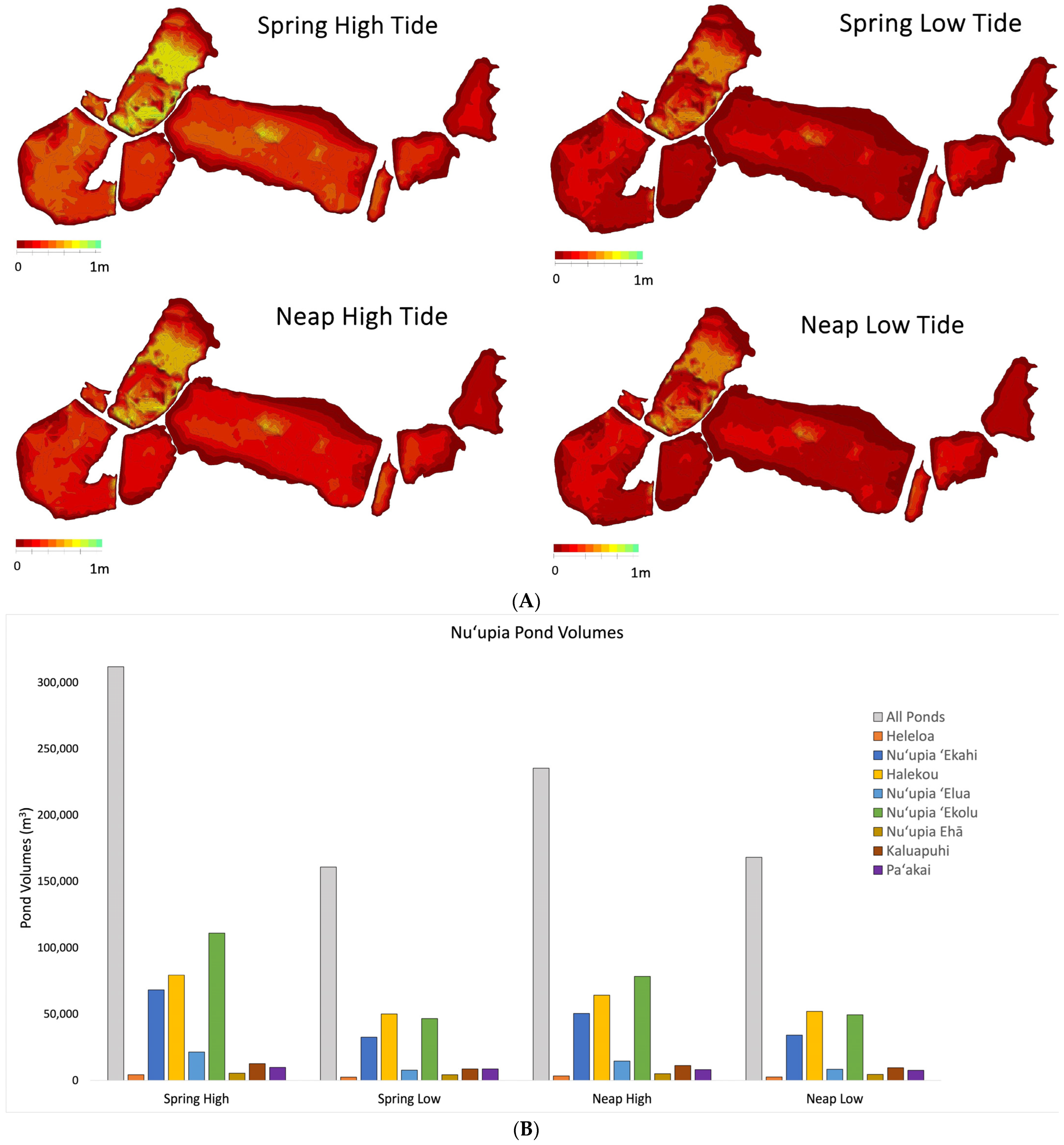
| All Ponds | 311,900 | 160,700 | 235,400 | 168,100 | 996,500 | 0.9 | 0.3 | 0.7 | 0.2 | 0.8 | 0.2 | 0.7 | 0.2 |
| Heleloa | 4270 | 2459 | 3381 | 2541 | 11,950 | 0.6 | 0.4 | 0.4 | 0.2 | 0.5 | 0.3 | 0.4 | 0.2 |
| Nuʻupia ʻEkahi | 68,320 | 32,530 | 50,520 | 34,170 | 200,600 | 0.7 | 0.3 | 0.5 | 0.2 | 0.6 | 0.3 | 0.5 | 0.2 |
| Halekou | 79,380 | 50,080 | 64,310 | 52,100 | 166,600 | 0.9 | 0.5 | 0.7 | 0.3 | 0.8 | 0.4 | 0.8 | 0.3 |
| Nuʻupia ʻElua | 21,350 | 7770 | 14,600 | 8390 | 78,740 | 0.4 | 0.3 | 0.2 | 0.1 | 0.2 | 0.3 | 0.2 | 0.1 |
| Nuʻupia ʻEkolu | 110,900 | 46,580 | 78,510 | 49,460 | 381,700 | 0.8 | 0.3 | 0.6 | 0.1 | 0.7 | 0.2 | 0.6 | 0.1 |
| Nuʻupia Ehā | 5375 | 4201 | 4983 | 4496 | 20,070 | 0.5 | 0.3 | 0.4 | 0.2 | 0.5 | 0.2 | 0.4 | 0.2 |
| Kaluapuhi | 12,570 | 8692 | 11,190 | 9590 | 67,140 | 0.4 | 0.2 | 0.3 | 0.1 | 0.4 | 0.2 | 0.4 | 0.1 |
| Paʻakai | 9730 | 8652 | 8118 | 7583 | 69,650 | 0.3 | 0.1 | 0.1 | 0.2 | 0.2 | 0.1 | 0.2 | 0.1 |
| Exchange Rates | Residence Time | Residence Time | ||||||
|---|---|---|---|---|---|---|---|---|
| Spring | Neap | Minimal | Maximal | Minimal | Maximal | |||
| Tide | Tide | Flushing Cycles | Flushing Cycles | Hours | Days | Hours | Days | |
| All Ponds | 48% | 29% | 7.0 | 13.5 | 169 | 7.0 | 269 | 11.2 |
| Heleloa | 42% | 25% | 8.5 | 16.0 | 203 | 8.5 | 320 | 13.3 |
| Nuʻupia ʻEkahi | 52% | 32% | 6.3 | 11.9 | 150 | 6.3 | 239 | 10.0 |
| Halekou | 37% | 19% | 10.0 | 21.9 | 239 | 10.0 | 437 | 18.2 |
| Nuʻupia ʻElua | 64% | 43% | 4.5 | 8.2 | 108 | 4.5 | 164 | 6.8 |
| Nuʻupia ʻEkolu | 58% | 37% | 5.3 | 10.0 | 127 | 5.3 | 199 | 8.3 |
| Nuʻupia Ehā | 22% | 10% | 18.5 | 43.7 | 445 | 18.5 | 874 | 36.4 |
| Kaluapuhi | 31% | 14% | 12.4 | 30.5 | 298 | 12.4 | 611 | 25.4 |
| Paʻakai | 11% | 7% | 39.5 | 63,5 | 948 | 39.5 | 1269 | 52.9 |
Disclaimer/Publisher’s Note: The statements, opinions and data contained in all publications are solely those of the individual author(s) and contributor(s) and not of MDPI and/or the editor(s). MDPI and/or the editor(s) disclaim responsibility for any injury to people or property resulting from any ideas, methods, instructions or products referred to in the content. |
© 2024 by the authors. Licensee MDPI, Basel, Switzerland. This article is an open access article distributed under the terms and conditions of the Creative Commons Attribution (CC BY) license (https://creativecommons.org/licenses/by/4.0/).
Share and Cite
Möhlenkamp, P.; Franklin, E.C.; McManus, M.A. Nuʻupia Ponds’ Water Circulation Characteristics: Exploring Water Exchange and Residence Time for Marine Ecosystem Management. Sustainability 2024, 16, 7159. https://doi.org/10.3390/su16167159
Möhlenkamp P, Franklin EC, McManus MA. Nuʻupia Ponds’ Water Circulation Characteristics: Exploring Water Exchange and Residence Time for Marine Ecosystem Management. Sustainability. 2024; 16(16):7159. https://doi.org/10.3390/su16167159
Chicago/Turabian StyleMöhlenkamp, Paula, Erik C. Franklin, and Margaret A. McManus. 2024. "Nuʻupia Ponds’ Water Circulation Characteristics: Exploring Water Exchange and Residence Time for Marine Ecosystem Management" Sustainability 16, no. 16: 7159. https://doi.org/10.3390/su16167159
APA StyleMöhlenkamp, P., Franklin, E. C., & McManus, M. A. (2024). Nuʻupia Ponds’ Water Circulation Characteristics: Exploring Water Exchange and Residence Time for Marine Ecosystem Management. Sustainability, 16(16), 7159. https://doi.org/10.3390/su16167159