1. Introduction
In the face of escalating climate change and its associated calamities, the urgent transition from fossil fuel-based energy systems to renewable sources stands out as a paramount endeavor for global sustainability and environmental preservation. The integration of renewable energy, notably solar and wind, into the power grid necessitates the development of robust transmission lines capable of handling increased loads and facilitating efficient energy distribution across vast regions [
1]. This shift is not merely an environmental imperative but also a strategic move to ensure energy security, reduce greenhouse gas emissions, and foster economic resilience in the face of the depleting fossil fuel reserves [
2]. Despite the critical benefits, the transition is fraught with challenges, including the need for substantial infrastructure overhaul, the integration of variable energy sources, and addressing the burgeoning electricity demands of modern societies [
2]. The urgency to act is further compounded by the stark warnings from scientific communities regarding the irreversible impacts of climate change, highlighting the need for immediate and decisive action to safeguard our planet for future generations [
3].
The existing body of research on renewable energy integration into power systems has laid a foundational understanding of the complexities involved in the transition. Modal analysis and sensitivity methods have been instrumental in assessing the effects of photovoltaic (PV) generation on power system stability, highlighting how increased PV penetration influences the damping of dominant modes and affects inter-area stability [
4]. These studies have significantly contributed to understanding the dynamic behavior of power systems with high levels of PV integration [
5].
Despite advancements, notable gaps persist in the research, especially regarding the comprehensive effects of very large-scale photovoltaic (VLS-PV) generation on power system performance. Although a number of studies have examined the frequency and voltage response of power systems to PV generation, there is a shortage of thorough analysis on how VLS-PV systems interact with the wider power grid. This includes investigating nonlinear behaviors, impacts on voltage stability, and overall system resilience to disturbances [
6,
7,
8,
9,
10,
11,
12]. The literature on integrating renewable energy into power grids serves as a detailed guide for energy practitioners, emphasizing the importance of addressing key questions and conducting in-depth analyses before implementing renewable integration strategies. Katz et al. [
13] highlighted the necessity of capacity expansion, production cost, and power flow analyses, taking into account various future scenarios to ensure a well-planned transition. This comprehensive approach is vital for the effective integration of renewables into the grid, stressing the need for detailed planning and scenario analysis to manage the complexities of renewable energy systems integration [
14].
Moreover, the integration of Battery Energy Storage Systems (BESS) alongside PV systems opens new avenues for stabilizing the grid against the inherent intermittency of solar energy. In particular, lithium-ion batteries have emerged as a cornerstone technology due to their superior energy density, longevity, and efficiency. Despite this potential, the economic aspects, including the cost and financial viability of large-scale storage solutions, remain areas needing further exploration. Additionally, variations in study findings attributed to differences in system modeling, scenarios of renewable installation, and disturbance analysis underscore the necessity for a more standardized and holistic approach to evaluating renewable integration impacts on power system performance [
13,
15].
In the context of Battery Energy Storage Systems (BESS), Bowen et al. [
16] provided insights into the pivotal role of BESS in enhancing grid stability and flexibility. Their study underscores the importance of scaling BESS in relation to the grid’s existing generation mix and the dynamic profiles of demand and renewables. It also delineates the critical attributes and services provided by BESS, such as energy arbitrage, firm capacity, and ancillary services, highlighting the economic and operational benefits of integrating BESS into the power system. Furthermore, Mobolaji Bello et al. [
17] provided practical examples through case studies, demonstrating the optimization of storage systems in terms of size, location, and operations, thereby showcasing the tangible benefits and challenges of BESS implementation in real-world settings.
The literature also addresses the economic considerations of energy storage, with studies by the Electric Power Research Institute [
18] and Kendall Mongird et al. [
19] comparing the costs and performances of various battery technologies. These studies advocate for lithium-ion batteries as the most cost-effective and high-performing option, despite ongoing supply chain challenges; additionally, the integration of renewables and BESS within regulatory frameworks such as the Saudi Grid Code [
20] and their impact on system stability and dynamics [
21,
22,
23] have been extensively discussed. These discussions highlight the complex balance between technological advancements, economic feasibility, regulatory compliance, and the overarching goal of establishing a sustainable and resilient power system as renewable energy sources become increasingly integrated [
24].
In summary, although substantial progress has been made in understanding the impacts of renewable energy integration on power systems, there is still a crucial need for comprehensive, detailed, and standardized research. This is vital for not only advancing technical knowledge but also guiding policy decisions, investment strategies, and infrastructure development plans to facilitate a smooth, efficient, and sustainable shift to renewable energy.
This paper aims to bridge the identified gaps through the following main contributions and objectives:
Comprehensive analysis of PV and BESS integration: We conduct an exhaustive study on the integration of PV systems and BESS into existing transmission systems across selected case studies (IEEE Test bus systems 9, 39, and 118), emphasizing dynamic effects and stability implications.
Impact assessment at various PV penetration levels: We evaluate the effects of varying PV penetration levels on power system parameters, including voltage, frequency, and power stability, while integrating BESS to mitigate stability issues.
Dynamic stability exploration: We investigate the dynamic stability of power systems under high PV penetration scenarios, focusing on frequency response and voltage stability as well as the role of BESS in enhancing system resilience.
Standardization of evaluation methodologies: We propose a standardized approach for assessing the impacts of PV system integration on power systems while considering the variability in system modeling and disturbance responses.
These objectives are designed to advance the understanding of PV, both integration with and without BESS, into transmission power systems in the context of the outstanding technical challenges in order to ensure a stable, efficient, and sustainable energy transition.
This paper’s structure beyond the introduction is as follows:
Section 2 delves into power system dynamics, covering models for transmission lines, PV systems, BESS, and analyses of power flow and dynamic stability;
Section 3 outlines a nine-step methodology for assessing PV and BESS integration into power systems;
Section 4 describes the simulation setup;
Section 5 examines the effects of varied PV penetration and BESS integration through IEEE 9, 39, and 118 bus system case studies, focusing on system stability and performance;
Section 6 presents case study results, showing how PV and BESS levels affect system voltage, frequency, and stability, especially under fault conditions; finally,
Section 7 concludes by advocating for PV and BESS integration as a strategy for enhancing grid stability and supporting renewable energy transition, stressing the importance of continued research to address challenges and optimize future grid operations.
2. Mathematical Modeling
The behaviour of electrical power systems is characterized mathematically by nonlinear differential–algebraic equations (DAEs), which offer a comprehensive framework for simulating and analysing system dynamics [
25].
2.1. Transmission Line Model
Transmission lines within transmission systems are commonly represented using the two-port network concept, which incorporates two sets of terminals. This two-port network is sometimes referred to as a four-terminal network or quadrupole network. In this framework, port 1 typically functions as the input port, while port 2 serves as the output port. A two-port network model is employed to analyze electrical circuits mathematically by breaking down larger circuits into smaller and more manageable segments. Conceptually, the two-port operates as a ‘black box’, with its properties defined by an input/output matrix. These networks are inherently linear, allowing the principle of superposition to be applied [
26]. The mathematical representation of the ABCD parameters is strongly dependent on the length of the transmission lines, as summarised in
Table 1.
2.2. PV System Model
This research utilizes Large-Scale Solar Photovoltaic (LSPV) plants, drawing insights from various sources. A key assumption of the model is the exclusion of dynamics associated with the DC side of the inverter system, including the PV array, the inverter’s DC link, and the voltage regulator. This simplification is made on the grounds that the time constants of these components are relatively short, requiring integration time constants that are impractically small for simulations, which complicates maintaining numerical stability in positive-sequence simulation environments. For load flow analysis, the model consolidates the AC side of the inverters into a single generator representation at a low voltage level. This voltage is then stepped up to match the internal medium-voltage collector grid and further elevated to integrate with the grid at the point of connection through one or more main step-up transformers, as shown in
Figure 1. This approach simplifies the simulation of LSPV plant interactions with the larger power system, making it more manageable and less computationally intensive [
27].
In this context, the inverters are typically modeled using a standard method in which they act as controllable sources of power injection for each individual phase. Overall, this approach outlines the inverter’s model as [
28]
where
stands for the three-phase apparent power of the PV system and
and
represent the active AC and reactive PV powers.
A basic inverter lacking an intelligent controller solely supplies active power while maintaining a unity power factor, leading to the equation
. The determination of
involves a couple of assumptions. Initially, the inverter efficiency can be ascertained for every given value of
as specified in the inverter’s datasheet. This efficiency is then multiplied by the DC PV power at the maximum power point (
) value, formulated as follows [
28]:
2.3. BESS Model
The Exact-MILP (Mixed Integer Linear Programming) formulation provides a comprehensive approach for managing a Battery Energy Storage System (BESS) within the power grid, emphasizing critical operational parameters for optimal utilization. It incorporates backlog energy, ensuring that unused energy is efficiently stored for future use, thereby managing the battery’s storage capacity. The model regulates charging and discharging rates to keep the BESS operating within its technical limits while optimizing performance. Additionally, it enforces minimum and maximum energy states to protect battery health and prolong lifespan. The operational modes of the BESS—charging, discharging, and idle—are controlled by the binary variables z and y, where represents charging, represents discharging, and represents an idle state. Importantly, the model includes a constraint to prevent simultaneous charging and discharging, ensuring that such physically impossible conditions are excluded from operational planning.
As an MILP this formulation introduces additional complexity; however, it is crucial for nuanced BESS management in the power system, ensuring strategic and efficient operation. The mathematical representation of the BESS state of charge (
e) can be provided as follows [
29]:
where
stands for the initial energy in the BESS,
and
represent the charging and discharging powers, and
and
are the charging and discharging efficiencies.
2.4. Power Flow Analysis
In modern power systems, managing bus voltages and power flow is essential. Because power flow is proportional to the square of the voltage, controlling both variables presents a nonlinear challenge. Power engineering employs power flow studies or load flow studies to numerically analyze the electric power flow within interconnected systems.
These studies typically involve steady-state analysis using simplified notation such as one-line diagrams and per-unit systems. They address various aspects of AC power parameters such as voltages, voltage angles, active power, and reactive power. Power flow analysis (PFA) is crucial during power system planning as well as during expansion and modifications to meet current and future load demands.
PFA helps to determine power flows and voltage levels under normal operating conditions, providing valuable insights into system operation and control setting optimization. This optimization aims to maximize capacity while minimizing operating costs. PFA is usually conducted under balanced three-phase steady-state conditions using specialized software such as PSSE, ETAP, CYME, Power World, or CAPE.
Such software calculates voltage magnitudes and phases at each bus in a power system along with real and reactive power flows (
P and
Q) for all loads, buses, and equipment losses. Load flow analysis is essential for optimizing existing system operations, planning future expansions, and designing new power systems, as it ensures efficient and reliable electricity transmission and distribution. The complex power equation can be represented as
where
is the complex power at bus
k,
is the active power at bus
k,
is the reactive power at bus
k,
is the voltage at bus
k,
is the admittance between bus
k and bus
m,
is the angle difference between bus
k and bus
m,
is the voltage at bus
m, and
is the voltage angle at bus
m.
Expanding the complex power summation into real and imaginary parts and associating these with
P and
Q, respectively, provides the fundamental PFA equations
where
is the voltage phase angle at bus
k.
2.5. Dynamic Stability Analysis
Dynamic stability refers to a system’s ability to remain stable amid sudden changes or disturbances such as short-circuits, generator losses, load fluctuations, or line tripping. In large-scale PV systems, significant power oscillations may occur but gradually dissipate. These oscillations mainly arise from imbalances between power demand and generation. In the local plant mode, a single generator oscillates relative to the rest of the system, affecting both the generator and the connecting grid line. For modeling, the system is often represented as a constant voltage source connected to the grid. Extensive simulations were conducted to evaluate the impact of the large-scale PV system on power system voltage stability. Dynamic stability analysis is essential for assessing the network’s stability amid continuous small disturbances, with load switching being a common example [
30].
Mathematical modeling for dynamic voltage stability analysis typically involves a set of differential and algebraic equations [
31], denoted as Equation (7) and Equation (8), respectively, where the system’s state vector is represented by ‘
x’ (state variable) and the bus voltages vector by ‘
y’ (algebraic variable). Additionally, the control variable is represented as
. These equations are dynamically solved using numerical integration and power flow analysis methods, providing insights into the system’s behavior under various conditions [
24].
To determine the steady-state equilibrium values (
,
) for small disturbances in the dynamic system, we set the derivative in Equation (7) to zero. Equation (7) and Equation (8) are then expressed as shown in Equation (9) and Equation (10) [
32]. By eliminating
, the linearized state equation can be represented as shown in Equation (11) and Equation (12). Dynamic voltage stability is achieved by minimizing the oscillation of the state and network variables. The magnitude of these oscillations can be expressed using the output vector in Equation (13), where
is the reference value of
y and the
matrix has distinct eigenvalues. Then,
is expressed by modes in Equation (14), where
is the
jth eigenvalue of
and
and
are the corresponding
and
eigenvectors. The output vector can be represented as shown in Equation (15) and Equation (16).
The error trajectory
is decomposed into several system modes [
33]. The voltage characteristics at each bus depend solely on the internal voltages and rotor angles, encapsulated in the matrix
[
34]. The system’s performance can be evaluated as follows:
where,
where
T is the integration time interval,
is the weighting matrix for the
jth state,
t denotes transpose, and ∗ signifies conjugate. This equation focuses on the model components related to internal voltage and rotor angle in order to streamline the calculations and reduce the computational time.
Dynamic voltage stability can be assessed by analyzing the eigenvalues of . To ensure practical results, dynamic stability is observed by simulating various parameters, including the network terminal voltage of the PV bus, generator’s angle, generator’s current and output electrical power, and terminal voltage at the weakest bus.
4. Simulation Setup
All of the studies were conducted using PSS/E software developed by Siemens. The network elements were modeled using PSS/E library models, with the Battery Energy Storage System (BESS) represented by the “CBEST“ and “PAUX1“ models as detailed in the manual [
35]. The “CBEST“ model, which simulates the battery, includes both an active power path and a reactive power path. The active power path accounts for power inefficiencies during energy storage and retrieval as well as AC current limitations on the part of the converter. This model requires an external input to define the battery’s function, provided by the frequency-sensitive “PAUX1“ model, which adjusts power output based on frequency deviations from the nominal value.
This research focuses on developing and performing stability assessments of grid-connected solar PV and BESS using three IEEE test systems. The studies were executed in PSSE, where bus systems were developed and analysed to determine their capacity for maintaining stability when integrated with solar PV. Both steady-state and dynamic stability analyses were conducted, and the PV system size was modeled in PSSE to assess stability. The goal was to identify the maximum possible PV power injection and the potential output of the PV plant. The PV generator bus was connected to the modeled bus system, and dynamic stability was evaluated to observe the PV generator’s behavior under various power generation scenarios.
In PSSE, the initial step involves determining the number of buses and their base KV in the grid system. Voltage limits must be set between 0.95 and 1.05 to prevent undervoltage issues. Buses are classified as either non-generator buses or generator buses depending on whether they are connected to generators. Loads can be placed on buses based on user requirements, representing factories and residential areas, but should not be placed near solar farms or conventional plants. This ensures stable output in the final analysis. The active and reactive loads can be adjusted to accurately represent these areas.
Generator parameters such as Pgen (power generation) and Pmax (maximum power output) can be set by the user. Each generator in this study was configured with different Pgen values, all of which were above 250 MW. During transient stability processes, Pgen can be gradually increased to determine the maximum potential output of the PV generator. This comprehensive approach ensures a thorough evaluation of the network’s stability and the impact of high PV penetration.
A short circuit study was performed to identify the fault level at each bus and determine the connection point of the PV system that was ideally the buses where the loads are connected. We used the ASCC Short Circuit method for performing short circuit studies, as mentioned in the System Strength and Inertia Report. As per the methodology, the short circuit fault level is always calculated on the three phase-to-ground fault, as this is the most onerous scenario resembling a bolted fault. The short circuit current calculated for the three phase-to-ground fault will be the highest, which helps in developing protection devices to withstand that level of current [
36].
5. Case Studies
In order to investigate issues around high PV penetration in the distribution network, IEEE 9, 39, and 118 bus systems were modeled using PSS/E software. The complete study was carried out using PSS/E software.
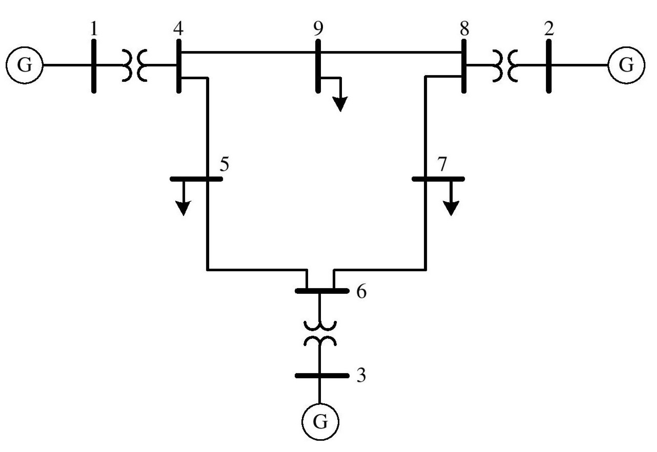
5.1. Case Study 1: IEEE 9-Bus System
The simulations were conducted using the IEEE 9-Bus Benchmark system. This system is composed of three conventional generators, six transmission lines, and three loads. The total power demand from these loads amounts to 321 MW, a figure used to calculate the level of wind power penetration [
37]. The Slack Bus is located at Generator 1 (G1), and the single-line diagram of the system is presented in
Figure 2.
The PV and BESS system were modeled based on the total load demand. The total load demand was around 305 MW. The PV inverters were modeled as generic photovoltaic inverters with high R and X values, as they do not contribute towards the short-circuit current during a fault. PV sizes were calculated based on the total load available. However, the BESS was added only for the 75% PV dispatch case.
Table 2 shows the power ranges of the machines at different PV penetration levels in the IEEE 9-bus system case.
Based on
Table 2, the PV system has been modeled in two machines in the 50% and 75% cases in order to understand the behavior of the network under two-machine response. In comparison, 100% PV was designed as a single machine in order to better understand the single machine response. The active and reactive power of the machines displayed here are for a single machine. The dispatch of the machines was based on the total load of the network. Based on the load, the machine dispatch was tuned to test dispatches at 10%, 25%, 50%, 75%, and 100%. The machines were tuned based on the power generation (Pgen). The QMax, QMin, and Mbase were calculated based on the Pgen of the machine. The Qmax and Qmin are usually 39.5% of the Pgen [
37].
With increasing PV penetration and existing synchronous generation, the MVA rating of the line during high demand seasons is pushed to its limits. PV dispatch during the day ensures that the batteries are being charged during the day.
At night, when there is no contribution from PV, the battery is used as a suitable replacement to meet demands. Batteries are also sometimes used to provide frequency support to the grid in case of a synchronous generator being out of service, or for any other special requirement.
The PV dispatch was based on the load of the system. For each scenario, the PV design was such that the PV dispatched a certain percentage of output, with the same amount being curtailed from the synchronous generators to maintain the balance in the system. With increasing MW dispatch, the active power and reactive power react independently. The reactive power is affected by the dip in voltage. The response was simulated when PV was added and any abruptness or instability was recorded.
5.2. Case Study 2: IEEE 39-Bus System
The IEEE 39-bus system shown in
Figure 3, commonly referred to as the ten-machine New England Power System, features Generator 1 as a representative example of a large aggregation of generators.
The PV and BESS system were both modeled based on the total load demand, which was around 5800 MW. The PV inverters were modeled as generic photovoltaic inverters with high R and X values, as they do not contribute towards the short-circuit current during a fault. PV sizes were calculated based on the total available load. The BESS was added for all PV dispatch cases.
Table 3 shows the BESS dispatch at different PV penetration levels in the IEEE 39-bus system case.
With the increase in PV and BESS penetration along with existing synchronous generation, the MVA rating of the line during high-demand seasons is pushed to its limits. PV dispatch during the day ensure that the batteries are being charged during the day.
At night, when there is no contribution from PV, the battery is used as a suitable replacement to meet demands. Batteries are also sometimes used to provide frequency support to the grid in case of a synchronous generator being out of service, or for any other special requirement. The PV dispatch was based on the load of the system. For each scenario, the PV and BESS were designed such that the PV dispatches a certain percentage of output, with the same amount being curtailed from the synchronous generators to maintain the balance in the system. With increasing MW dispatch, the active power and reactive power react independently. The reactive power is affected by the dip in voltage. The response when the PV and BESS were added was simulated and any abruptness or instability was recorded.
5.3. Case Study 3: IEEE 118-Bus System
The IEEE 118-bus test case serves as a simplified model of the American Electric Power system as it was in December 1962, focusing on the US Midwest region. This model includes 19 generators, 35 synchronous condensers, 177 lines, 9 transformers, and 91 loads. It is important to note that the base kilovolt (KV) levels assigned to the bus names are based on estimates [
38]. Moreover, the line megavolt–ampere (MVA) limits were not originally provided with the data, and have been subsequently approximated [
39]. As a test case, this system features numerous voltage control devices, demonstrating robust performance and the ability to converge within approximately five iterations using a fast decoupled power flow method. The single-line diagram of the IEEE 118-bus system case is illustrated in
Figure 4.
The PV and BESS unit were modeled based on the total load demand, which was around 3817 MW. The PV inverters were modeled as generic photovoltaic inverters with high R and X values, as they do not contribute towards the short-circuit current during a fault. PV sizes were calculated based on the total available load. The BESS was added for all PV dispatch cases.
Table 4 shows the BESS dispatch at different PV penetration levels.
With the increase in PV and BESS penetration and existing synchronous generation, the MVA rating of the line during high-demand seasons is pushed to its limits. The PV dispatch during the day ensures that the batteries are being charged during the day. At night, when there is no contribution from PV, the battery is used as a suitable replacement to meet demands. Batteries are also sometimes used to provide frequency support to the grid in case of a synchronous generator being out of service, or for any other special requirement.
The PV dispatch was based on the load of the system. For each scenario, the PV and BESS were designed such that the PV dispatches a certain percentage of output, with the same amount curtailed from the synchronous generators to maintain the balance in the system. With increasing MW dispatch, the active power and reactive power react independently. The reactive power is affected by the dip in voltage. The response when the PV and BESS were added was simulated and any abruptness or instability was recorded.
6. Results and Discussions
This section delves into the comprehensive results derived from the case studies conducted on the IEEE 9-bus, 39-bus, and 118-bus systems. The investigations primarily focus on the dynamic and steady-state performance of these systems under varying levels of PV penetration and the integration of BESS units. Through meticulous modeling and simulation, the analysis provides insights into the impacts of renewable integration on power system stability, voltage levels, and frequency response, highlighting the challenges and benefits of transitioning towards more sustainable energy solutions.
6.1. Case Study 1: IEEE 9-Bus System
This study evaluates the system’s behavior under different scenarios of PV and BESS penetration in the IEEE 9-bus system, assessing key parameters such as voltage stability, thermal loading, and dynamic response to grid disturbances. Through detailed simulations, the findings underscore the critical role of BESS in maintaining grid stability and the potential of PV systems to fulfill load demands while ensuring operational efficiency and reliability.
6.1.1. Modeling Scenarios
As per the methodology outlined above, with increasing PV dispatch, the load was increased by 5% and the synchronous generation was curtailed by 10% to account for future projections and identify the capability of the retirement of conventional generators towards greener grids. Here, the modeling scenarios of different PV and BESS penetration levels along with their location as well as the load and conventional generators at each scenario are listed in
Table 5.
6.1.2. Steady State Assessment
Thermal overloading corresponds to the MVA capacity of the line. The line rating varies based on the temperature and ambient conditions. As the line rating varies, the overloading can increase or decrease based on the MVA ratings. The loadings shown below are within the MVA ratings of the line [
36].
Under steady-state assessment, we look for line loading and thermal violations across the network as well as the voltage at the buses. For the considered scenarios, we have performed analysis of the thermal overloading and bus voltages. The following conditions should be satisfied:
In this context, the loadings for each line for different PV penetration cases are listed in
Table 6. In addition, the voltage levels per unit at different PV penetration are summarized in
Table 7.
6.1.3. Dynamic Assessment
To demonstrate the dynamic behavior, a bus fault was applied. The following fault types were simulated in the network surrounding the PV system.
Three phase-to-ground fault: The line segments from the faulted bus were opened in the local clearing times specified.
Disturbances were applied using “psspy.dist_3phase_bus_fault()” for balanced faults. The fault was immediately cleared in the specified protection clearance times. If the contingency involved inter-trips or caused additional network elements to disconnect, then these items were not reclosed/reconnected.
After initialization, the machine was run flat until 5 s. After 5 s, the fault was introduced for 0.12 s, then was cleared. After fault clearance, the branch associated with the bus was tripped [
36]. The fault clearance times are based on the voltage levels; for voltage level above 100 kV and less than 250 kV, they have a clearance time of 0.12 s, as mentioned in the National Electricity Rules [
40]. In all the cases, the fault was applied to branch 5–6, as this was the branch closest to the highest penetration of the BESS and PV machines. Using the closest fault to the machine is more prudent and makes it less onerous to examine the response of the machine to the system’s stability [
36].
All of the scenarios listed in
Table 5 were analysed; however, in this section we are focused on those that significantly impact the voltage and frequency stability. A summary of what our findings from each scenario can is provided in the findings section.
6.2. Case Study 2: IEEE 39-Bus System
This section investigates the IEEE 39-bus system. The analysis concentrates on understanding the impact of various levels of PV and BESS integration on the system’s voltage profiles, power flows, and stability during both steady-state and dynamic conditions. By simulating realistic scenarios, this study aims to highlight the challenges and opportunities associated with high renewables penetration, emphasizing the importance of strategic BESS deployment for enhanced grid stability.
6.2.1. Modeling Scenarios
As per the methodology mentioned above, with increasing PV dispatch, the load was increased by 5% and the synchronous generation was curtailed by 10% to account for future projections and identify the capability of the retirement of the conventional generators towards greener grids. Here, the modeling scenarios of different PV and BESS penetration along with their locations as well as the load and conventional generators for each scenario are listed in
Table 8.
6.2.2. Steady-State Assessment
Steady-state assessment was carried out to calculate line ratings and voltage deviations for the buses. We observed overloading on the lines where the battery storage penetration was 50%. For cases with less than 50% penetration, no thermal overloading occurred in the surrounding network. For bus voltage deviation, all monitored network voltages remained with 0.9 p.u. to 1.1 p.u. post-contingency. The largest network voltage deviation was observed to be less than 0.05 p.u.
6.2.3. Dynamic Assessment
Dynamic assessment was carried out following the same methodology as for the 9-bus system. For a three phase-to-ground fault, the model was simulated by performing a flat run until 5 s and then following it with a fault. The fault was then cleared and the model was run until 30 s.
The fault clearance times were based on the voltage levels and had a clearance time of 0.12 s for voltage level above 100 kV and less than 250 kV, as mentioned in the National Electricity Rules [
40]. In all the cases, the fault was applied to branch 5–6, as this is the closest branch to the highest penetration of the BESS and PV machines. Using the closest the fault to the machine is more prudent and makes it less onerous to examine the response of the machine to the system’s stability [
36].
Every scenario outlined in
Table 7 underwent thorough analysis. This section shines a spotlight on the scenarios that significantly influence voltage and frequency stability, offering critical insights. For a comprehensive overview of our discoveries across all scenarios, please refer to the findings section, where the essence of our research is distilled.
Base Case
The base case was tested for the same contingency in order to analyze the response of the base system without the addition of PV or BESS in the system. In this case, the voltage, frequency, and active and reactive power were simulated, analysed and reported, as shown in
Figure 9.
The voltage remains steady and stable pre- and post-fault when applying the fault on branch 5–6 without integrating PV and BESS, as shown in
Figure 9a. In the base case, the frequency response is stable at 50 Hz after removing the fault, as illustrated in
Figure 9b. The active power response remains stable after the fault is cleared, as shown in
Figure 9c. The reactive power settles after the fault is cleared in the base case, as shown in
Figure 9d.
25% PV with 10% BESS penetration
Here, the asynchronous generation (PV) is at 25% of the load and the Battery Storage System is tuned to 10% of the PV. In this case, the voltage, frequency, and active and reactive power have been simulated, analysed, and reported, as shown in
Figure 10.
The voltage returns to its pre-fault levels. Voltages at certain buses exceed the 0.9–1.1 p.u. range, as shown in
Figure 10a. The frequency remains stable and is maintained within the permitted frequency band of 48.985–50.015 Hz, as illustrated in
Figure 10b. The active power returns to its pre-fault value after the fault is cleared. The response appears to be stable and achieves steady state within 5 s after fault clearance, as depicted in
Figure 10c. The reactive power is maintained near 0 Mvar before pre-fault condition. This enables the plant to inject reactive power in case of a fault, as illustrated in
Figure 10d.
50% PV with 50% BESS penetration
In this scenario the asynchronous generation (PV) dispatch is at 50% of the load and the Battery Storage System is tuned to 50% of the PV. Here, the voltage, frequency, and active and reactive power have been simulated, analysed, and reported, as shown in
Figure 11.
The voltage is within the 0.9–1.1 p.u. band. The response appears to be stable and the voltage returns to its pre-fault values, as shown in the
Figure 11a. The frequency remains stable and is maintained within the permitted frequency band of 48.985–50.015 Hz, as shown in
Figure 11b. The reactive power is stable and appears to achieve the pre-fault level, as shown in
Figure 11c. The active power returns to its pre-fault value after the fault is cleared. The response appears to be stable and achieves steady state within 5 s after fault clearance, as depicted in
Figure 11d.
100% PV with 50% BESS penetration
In this scenario, the asynchronous generation (PV) dispatch is at 100% of the load and the battery storage system is tuned to 50% of the PV. Here, the voltage, frequency, and active and reactive power have been simulated, analysed, and reported, as shown in
Figure 12.
The voltage starts to drop because of low system strength, as shown in
Figure 12a. The frequency starts to fluctuate because of lack of inertia in the system because there is no synchronous generation online, as shown in
Figure 12b. The active power starts to increase because of the drop in frequency. This is expected; as the frequency deviates from the set value, the active power adjusts itself, as depicted in
Figure 12c. The reactive power and the voltage interact with each other. The change in voltage results in an abrupt change in the reactive power, as shown in
Figure 12d.
6.3. Case Study 3: IEEE 118-Bus System
In this section, we delve into the results from the extensive analysis of the IEEE 118-bus system, exploring the effects of substantial PV and BESS integration. This study meticulously examines the system’s resilience to voltage fluctuations and dynamic stability under varying PV and BESS penetration levels. The findings contribute valuable insights into managing large-scale PV integration, showcasing the pivotal role of advanced BESS solutions in ensuring the seamless operation and stability of future power grids.
6.3.1. Modeling Scenarios
As per the methodology mentioned above, with increasing PV dispatch, the load was increased by 5% and the synchronous generation was curtailed by 10% to account for future projections and identify the capability of the retirement of the conventional generators towards greener grids. Here, the modeling scenarios of different PV and BESS penetration levels along with their location as well as the load and conventional generators for each scenario are listed in
Table 9.
6.3.2. Steady-State Assessment
Steady-state assessment was carried out to calculate line ratings and voltage deviations for the buses. We observed overloading on the lines where the battery storage penetration was 50%. For cases with less than 50% penetration, no thermal overloading occurred in the surrounding network. For bus voltage deviation, all monitored network voltages remained within 0.9–1.1 p.u. post-contingency. The largest network voltage deviation was observed to be less than 0.05 p.u.
6.3.3. Dynamic Assessment
Dynamic assessment was carried out following the same methodology as for the 9-bus and 39-bus systems. For a three phase-to-ground fault, the model was simulated by performing a flat run until 5 s, then following it with a fault. The fault was cleared and the model was run until 30 s. In all the cases, the fault was applied to branch 5–6, as it was the closest branch to the highest penetration of the BESS and PV machines. Using the closest the fault to the machine is more prudent and makes it less onerous to examine the response of the machine to the system’s stability.
Every scenario outlined in
Table 8 underwent thorough analysis. This section shines a spotlight on the scenarios that significantly influence voltage and frequency stability, offering critical insights. For a comprehensive overview of our discoveries across all scenarios, please refer to the findings section, where the essence of our research is distilled.
Base Case
The base case was tested for the same contingency in order to analyze the response of the base system without the addition of PV or BESS in the system. In this case, the voltage, frequency, and active and reactive power have been simulated, analysed, and reported, as shown in
Figure 13.
The voltage remains steady and stable pre- and post-fault when applying the fault on branch 5–6 without integrating PV and BESS, as shown in
Figure 13a. In the base case, the frequency response stable at 50 Hz after removing the fault, as illustrated in
Figure 13b. The active power response remains stable after the fault is cleared, as shown in
Figure 13c. The reactive power settles after the fault is cleared in the base case, as shown in
Figure 13d.
50% PV with 50% BESS penetration
In this scenario, the asynchronous generation (PV) dispatch is at 50% of the load and the battery storage system is tuned to 50% of the PV. Here, the voltage, frequency, and active and reactive power have been simulated, analysed, and reported, as shown in
Figure 14.
The voltage drop and variations of certain buses exceed the 0.9–1.1 p.u. band. The voltage returns to its pre-fault levels, as shown in
Figure 14a. The frequency remains stable and is maintained within the permitted frequency band of 48.985–50.015 Hz, as shown in
Figure 14b. The active power appears to settle to the pre-fault levels once the fault is cleared and reaches steady state within 5 s, as shown in
Figure 14c. The reactive power returns to pre-fault values after the fault is cleared and remains stable, as illustrated in
Figure 14d.
75% PV with 50% BESS penetration
In this scenario, the asynchronous generation (PV) dispatch is at 75% of the load and the battery storage system is tuned to 50% of the PV. Here, the voltage, frequency, and active and reactive power have been simulated, analysed, and reported, as shown in
Figure 15.
The voltage response appears to be stable and within the 0.9–1.1 p.u. band post-fault, as illustrated in
Figure 15a. The frequency remains stable and is maintained within the permitted frequency band of 48.985–50.015 Hz, as shown in
Figure 15b. The active power appears to settle to the pre-fault levels once the fault is cleared and reaches the steady state within 5 s, as shown in
Figure 15c. The reactive power returns to pre-fault values after the fault is cleared and remains stable, as illustrated in
Figure 15d.
100% PV with 50% BESS penetration
In this scenario, the asynchronous generation (PV) dispatch is at 100% of the load and the battery storage system is tuned to 50% of the PV. Here, the voltage, frequency, and active and reactive power have been simulated, analysed, and reported, as shown in
Figure 16.
The voltage settles to the pre-fault value after the fault is cleared, and the steady state is achieved within 5 s of fault clearance, as shown in
Figure 16a. The frequency deviates but maintains stability within the permitted frequency band of 48.985–50.015 Hz, as illustrated in
Figure 16b. The active power returns to the pre-fault value, as shown in
Figure 16c. The reactive power remains stable and maintains its pre-fault value after fault clearance, as depicted in
Figure 16d.
In the scenarios where PV systems were integrated into the grid without additional battery storage, voltage levels remained stable at 1 per unit, enhancing voltage support across the board. Even amid minor fluctuations due to the variable output from the PV systems, the frequency stayed within a tight range of 49.985–50.015. Active power dispatch demonstrated stability without any significant spikes or instability, and reactive power was effectively managed, allowing for the injection of reactive current whenever necessary, thereby improving voltage control.
The inclusion of BESS with PV systems markedly improved the grid’s overall stability. This combination not only bolstered voltage support, contributing to a more stable transmission network, but also maintained an exceptionally stable frequency, with BESS providing critical frequency control and effectively acting as virtual synchronous machines. The ability of the batteries to store excess solar energy during low demand periods and release it during times of peak demand allowed for more efficient management of load variability. Moreover, this integration ensured a consistent supply of reactive power, facilitating a smoother incorporation of renewable energy sources by mitigating fluctuations in reactive power output.
The support provided by the BESS proved essential for rapid system stabilization and addressing power deficits. Analysis of the three case studies illustrates that increasing battery dispatch can enhance system stability in the following ways:
25% BESS: Supported by a robust infinite grid and a significant presence of synchronous generation, the voltage, frequency, active power, and reactive power all remain stable, ensuring that dispatch and demand are primarily balanced by synchronous plants.
50% BESS: Stability is similar to the case with 25% BESS, with a strong infinite grid and substantial synchronous generation maintaining steady voltage, frequency, active power, and reactive power.
75% BESS: As asynchronous generation begins to dominate, minor signs of instability appear in voltage, frequency, active power, and reactive power due to a weakened infinite grid and reduced synchronous generation, with demand largely met by asynchronous sources.
100% BESS: This scenario exhibits the greatest instability and oscillation in system parameters, resulting from a weakened infinite grid and minimal to no synchronous generation. The demand is fully met by PVs and BESS, leading to reduced reliability and sudden changes in system behaviour due to low inertia and strength.
However, the addition of more battery storage to the PV system introduced specific challenges. Voltage stability was compromised, underscoring the need for synchronous generation to be actively online within the current transmission network. Frequency stability also suffered, with significant deviations from the desired range due to reduced system inertia. Active power dispatch faced fluctuations, highlighting the absence of synchronous generation to aid in maintaining frequency stability. Likewise, reactive power experienced oscillatory responses due to voltage deviations, affecting the system’s capacity to manage reactive power effectively when voltage levels dropped below acceptable thresholds.
7. Conclusions
This study analysed the impact of high photovoltaic (PV) penetration in power networks using IEEE 9-bus, 39-bus, and 118-bus systems. Key findings show that integrating PV with Battery Energy Storage Systems (BESS) significantly enhances voltage stability and system resilience. For example, with 75% PV penetration and BESS support the voltage stability improved, effectively managing grid disturbances. BESS units are crucial for maintaining frequency stability in scenarios with high levels of renewables.
Our simulations revealed that PV penetration levels of 50% and above improve voltage profiles and reduce voltage fluctuations due to the stabilizing effect from BESS. In the IEEE 39-bus system with 50% PV and 50% BESS, voltage stability was within the operational range of 0.9-1.1 p.u. during normal and fault conditions. In the IEEE 118-bus system, 75% PV penetration with 50% BESS utilization showed rapid recovery from disturbances with minimal impacts on frequency and voltage.
Higher PV integration increases reliance on BESS for maintaining power quality and system reliability. BESS compensates for solar power intermittency and provides essential services such as peak shaving and load leveling that are crucial for managing high renewable penetration challenges.
Our results underscore the strategic importance of synchronized PV and BESS deployment to support the transition to renewable energy sources and achieve long-term energy sustainability and grid stability.
Future research should focus on optimizing BESS configuration and scaling, investigating the long-term impacts of high renewable penetration on grid infrastructure, and developing predictive models for accurate forecasting under variable renewable outputs. Additionally, integrating other renewable sources such as wind and hydro with PV systems could enhance grid resilience and sustainability.


