Evaluation of the Effectiveness of Solar Array Simulators in Reproducing the Characteristics of Photovoltaic Modules

Abstract

The search for energy alternatives in the face of growing global demand highlights solar energy as a promising and sustainable option that is fundamental in reducing carbon emissions and mitigating climate change. In this context, inverters play a key role in connecting and distributing solar energy, requiring certification through specific tests. Given environmental unpredictability and economic challenges, the use of Solar Array Simulators (SASs) is recommended to accurately replicate the behavior of photovoltaic modules under various conditions. This study analyzes the static and dynamic performances of SASs with the aim of ensuring a faithful reproduction of module behavior in real situations under both steady-state and transient conditions. The primary focus is to ensure that experimental results are reliable and representative, promoting the implementation of more efficient energy solutions. Additionally, this study discusses the importance of optimizing inverter controllers to reflect the more realistic dynamics provided by SASs.

1. Introduction

The search for alternative energy sources has intensified in response to the global increase in energy demand driven by technological progress, industrial growth, and population expansion [1,2]. Additionally, factors such as global warming, the depletion of fossil fuels, and environmental pollution have heightened the importance of renewable energy sources [3,4]. This scenario has raised concerns about the exhaustion of conventional energy reserves and the associated environmental impacts, such as pollution [5]. In this context, solar energy has attracted significant global attention due to its vast potential. It stands out as an environmentally friendly option, free from environmental threats and aligned with sustainability principles [6,7,8].

A inverter is an essential component of a grid-connected photovoltaic (PV) system responsible for converting the energy generated by solar panels into a suitable form to be injected into the grid [9]. However, before implementing energy converters in practice, it is essential to subject them to a series of comprehensive tests to evaluate their ability to withstand different faults and disturbances in the grid, thereby ensuring their reliability. In the context of tests in real environments, solar inverter manufacturers face challenges related to the high costs involved and the complex space requirements, especially regarding tests conducted in laboratories [1,5,7,10,11]. Photovoltaic inverters are subjected to a series of exhaustive tests to ensure the optimal efficiency of these products when exposed to real situations. In addition to the tests provided for in standards, manufacturers committed to high quality standards carry out extra tests to ensure that under no circumstances do the products fail to meet the reliability levels demanded by the market. Furthermore, a second obstacle arises due to the variable and unpredictable nature of solar irradiation throughout the day, with its fluctuating and difficult-to-predict levels [5,7,11].

Several research studies are developed each year in this area of knowledge, usually evaluating the impact of different configurations of static converters or different MPPT (Maximum Power Point Tracking) techniques on solar generation [8,12,13,14]. However, in general, the availability of an adequate system for experimental validation impacts the readiness of research in real-time PV solar systems. Therefore, in theory, to enable research in this area, it is essential to have PV modules (Figure 1a) in an environment with a controllable light spectrum [7]. However, it is important to realize that this solution typically incurs high costs and is bulky and difficult to alter in order to conduct multiple tests considering changes in shading conditions, arrangements, or characteristics of the PV modules.

As a viable alternative, the IEC 61683 standard proposes the use of a device known as a solar array simulator (SAS) (Figure 1b) during certification tests [9]. In this standard, the concept of an SAS is defined as “a simulator that has an equivalent I × V characteristic to a PV array”. Additionally, this document provides guidelines for conducting tests and efficiency trials of inverters, as well as definitions of measurement instruments, along with their uncertainty ranges and necessary precision. Unlike conventional methods, an SAS offers the advantage of eliminating both spatial and temporal constraints, allowing for the necessary tests to meet standard requirements [5]. Thus, a PV emulator emerges as a highly useful and sustainable tool for assessing the performance of energy converters during design and development phases, providing a more efficient and flexible approach [7].

The PV emulator plays a fundamental role in the experimental phase of solar energy generation system development. Its function is to act as a nonlinear power supply, accurately reproducing the characteristics of the current–voltage (I–V) curve of PV modules [9,11]. By simulating desired conditions in a laboratory environment, such as solar irradiance, temperature, and partial shading, the PV emulator allows for repeatable and efficient testing. This provides flexibility to work with different power levels and test inverters with various nominal powers [5,9,11]. Just as they are employed in the validation and testing of equipment like inverters for PV energy generation, PV emulators are also used to study specific module behaviors or simulate module arrays in the application of MPPT techniques and other tests without the need to acquire the modules and install a complete system.

Because of these applications, it is extremely important to ensure that this equipment behaves in a similar way to real photovoltaic modules at all times, both when the source is in a steady state and in transient situations. In this way, it is possible to obtain reliable and representative results during experiments carried out with a PV emulator. Therefore, the main objective of this article is to carry out a comprehensive comparison of the performance of different commercial emulator sources in a variety of different scenarios. Thus, the central focus of this analysis is to examine both the static and dynamic behavior of these sources in order to determine whether they are capable of reliably representing a real photovoltaic module.

This article is organized as follows: Section 2 describes the basic functions of commercial SASs. Section 3 describes the methodology used in this study and the characteristics of the evaluated sources, while Section 4 describes the experimental setup. The static and dynamic behaviors of the evaluated PV emulator sources are presented in Section 5. Finally, in Section 6, the main conclusions of this work are presented.

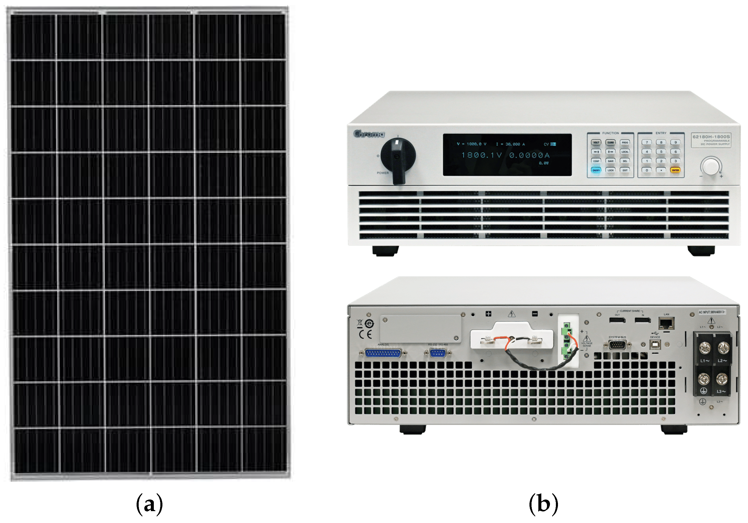
2. Solar Array Simulator

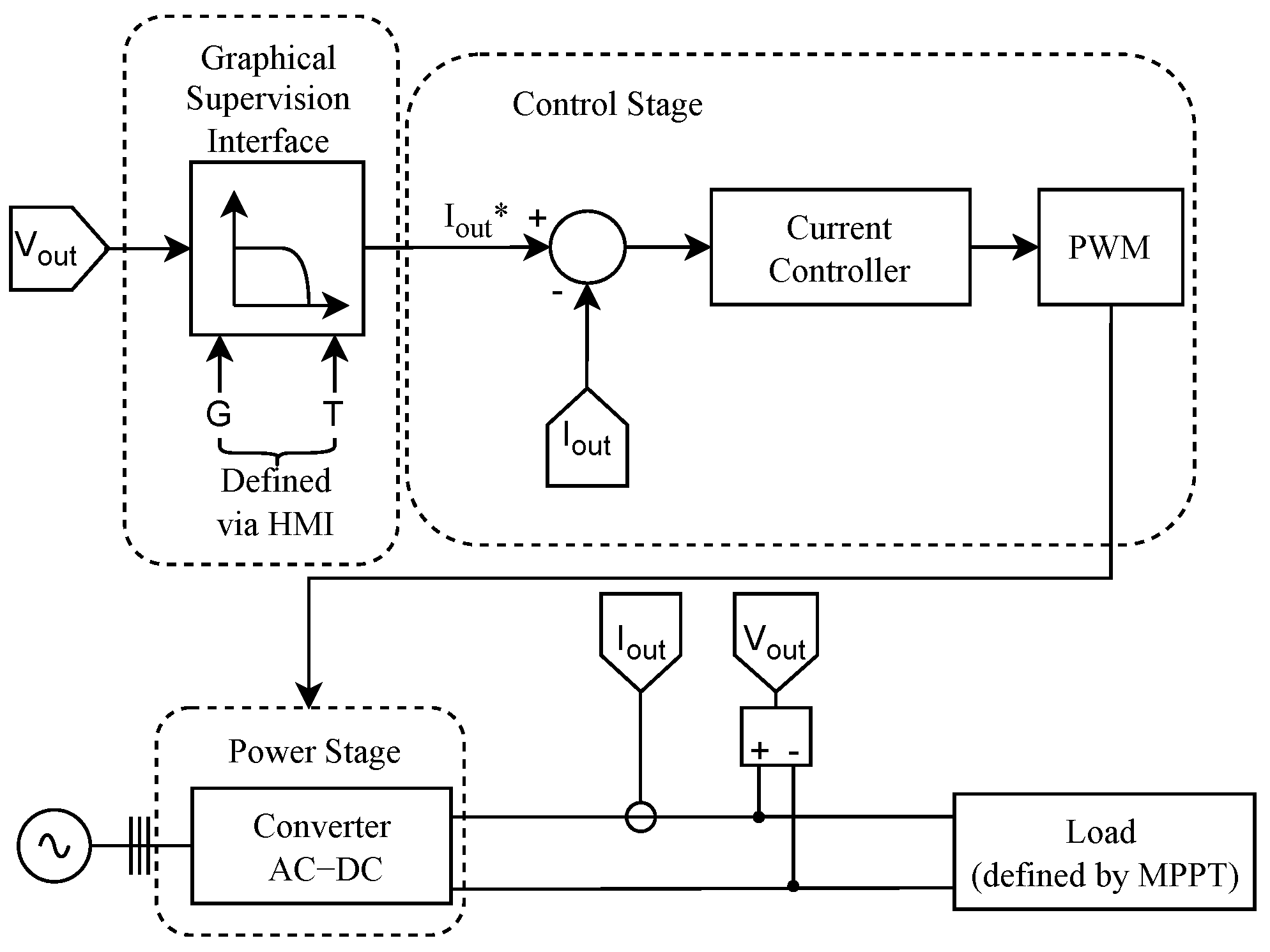
An SAS (Solar Array Simulator) is a power electronic converter designed to accurately reproduce the output characteristics of a real solar array under various operating conditions. Some of the conditions that can be evaluated include shading, temperature, irradiance, and other variables affecting the performance of solar panels, ensuring flexibility and adaptability to different photovoltaic systems [15]. SAS systems are composed of various components, such as IGBTs, relays, current and voltage sensors, inductors, capacitors, and fuses [16]. The desired PV curve to be synthesized by an SAS can be implemented using the PV curve of any technology, including, for example, flexible organic photovoltaics [17,18].

In SAS, the I–V (current–voltage) characteristic curve that characterizes a PV module can be generated using a lookup table or a PV model, allowing for accurate simulation of the solar panel’s behavior [19]. With this, engineers and researchers can evaluate and compare the performance of different PV systems, making it easier to make decisions about the design and implementation of these systems.

In general, SASs are implemented using controlled DC sources. The buck–boost converter is one of the topologies used in the implementation of SASs and is used under GMPP [20] tracking conditions. Other converters can be used for the same application, such as Cúk or Sepic, but they are more expensive and more complex than the buck–boost converter. Thus, an SAS is made up of three main components, as shown in Figure 2, namely the power stage, the control stage, and the graphical supervisory interface. These three components and the common operating characteristics of commercial SASs are briefly described below.

2.1. Power Stage

Regarding the power stage, it can be classified according to the type of converter used, whether a linear power converter or a switched-mode power converter. Although linear circuits can offer fast dynamic responses, they have low efficiency, a limited power range, high heat dissipation, and bulky dimensions, making them unsuitable for high-power applications. Therefore, in high-power converters including the power stage of an SAS, a switched-mode power converter is used to generate the desired voltage–current waveform at the output [5].

2.2. Control Stage

In terms of control, an SAS aims to replicate the I–V characteristic of a PV module, where the output current must be carefully controlled. The current reference is calculated based on the output voltage, which is controlled by an external static converter connected to the output of the emulating source. However, calculating the current reference can be complex due to the nonlinear behavior of PV modules [9].

To achieve this goal, two control loops are usually employed. The inner loop is responsible for controlling the output current of the SAS, while the outer loop generates the reference for the inner loop. This control structure ensures precise and reliable operation of the emulating source, allowing it to faithfully reproduce the characteristics of a real PV module [5]. This approach is important to ensure reliable and accurate results during simulations and tests conducted with the source.

The outer loop is often implemented using lookup tables. These lookup tables are typically defined by the user in the graphical user interface of the emulating source’s supervision system.

2.3. Graphical Supervision Interface

The graphical supervision interface allows the user to define the environmental operating conditions and parameters of the real PV module or array to be emulated. Based on these user-provided specifications, an SAS can generate the nonlinear output characteristics of a real module [5]. Furthermore, some manufacturers allow users to define gain values for different control loops of the source through the graphical supervision interface. Finally, source control and monitoring software enable real-time generation, measurement, and display of maximum power tracking status, in addition to recording values for subsequent analysis, as shown in Figure 3.

Figure 3 presents four interfaces from different manufacturers, revealing a level of similarity between them. In all of them, the reference I–V and PV curves can be observed. These curves are used as inputs for simulations (both for shading conditions), as shown in Figure 3b, and for ideal conditions, as illustrated in Figure 3c. Additionally, an editable lookup table can be observed in Figure 3d.

2.4. Common Characteristics of SASs

SASs are often used to perform static and dynamic MPPT tests, which are essential to ensure the efficiency of PV systems. Alongside the hardware, emulating sources feature user-friendly software with various simulation options, each with its own characteristics and unique applications (referred to above as graphical supervision interface). In this context, these systems have a set of common characteristics across all manufacturers, such as the following:

• An internal algorithm that generates an I–V points table based on input parameters of the PV module, such as open-circuit voltage ($V_{oc}$), short-circuit current ($I_{sc}$), current at maximum power point ($I_{mp}$), and voltage at maximum power point ($V_{mp}$). This feature allows for a quick and easy approximation of the curve without the need for a computer to perform the simulation;
• An algorithm that allows the user to define a custom table of points to determine the I–V curve (user-defined lookup table). This feature enables users to have full control over the simulation and create specific tables for their project needs. Additionally, custom tables can be stored in the system’s internal memory, making it easy to access and reuse in future simulations;
• A shading mode that allows for simulation of shadow conditions, enabling the evaluation of their impact on the energy production of PV systems. The list mode is used to generate a list of operation points of the I–V curve of a PV module under different conditions, which is essential for determining the module’s efficiency in different situations.

When choosing an SAS, it is important to consider the specific needs of the project and application. The selected simulation mode should offer accuracy and flexibility to evaluate the performance of the PV system under different conditions. Additionally, the ability to store and reuse lookup tables can save time and increase the efficiency of the simulation process.

3. Methodology and Characterization of the Evaluated SAS

In order to evaluate both the static and dynamic behavior of the SAS in relation to the faithful representation of a PV module, a comprehensive series of scenarios are considered in this study. These scenarios encompass a variety of situations that can influence the performance of emulator sources. The following scenarios are evaluated:

• Steady-state operation: In this scenario, the SASs are tested under stable operating conditions, considering PV modules subject to constant solar irradiation and a constant temperature. By doing so, it becomes possible to evaluate how the sources respond and follow the global maximum power point (GMPP) in a steady state.
• Shading-induced curve change: This scenario simulates a situation where part of the PV module is shaded, resulting in a change in its characteristic power curve. By doing so, it becomes possible to assess how emulating sources respond to this change and whether they can properly track the new maximum power point.
• Performance during curve transitions: In this scenario, rapid and smooth transitions between different operating points of the PV module are considered. This can occur, for example, due to rapid changes in solar irradiation or ambient temperature. By doing so, it becomes possible to analyze whether emulating sources can accurately follow these transitions and capture variations in the GMPP.

By exploring these different scenarios, it is possible to carry out a comprehensive analysis of the performance of commercial SASs, identifying their capabilities and limitations with regard to faithfully representing the behavior of a photovoltaic module. Consequently, this study contributes to the advancement of research and development in this area, providing valuable information for the development of more efficient and reliable SASs, as well as for the analysis of the impact of using commercial SASs to validate GMPP tracking techniques.

Characterization of the Evaluated Emulating Sources

In this study, the main focus is on SASs, which play a key role in the laboratory environment by emulating the behavior of photovoltaic modules. To carry out the necessary investigations, two commercial SASs were used. For ethical reasons, these sources are referred to in this work as SAS A and SAS B. Below is a brief description of the characteristics of these emulation sources.

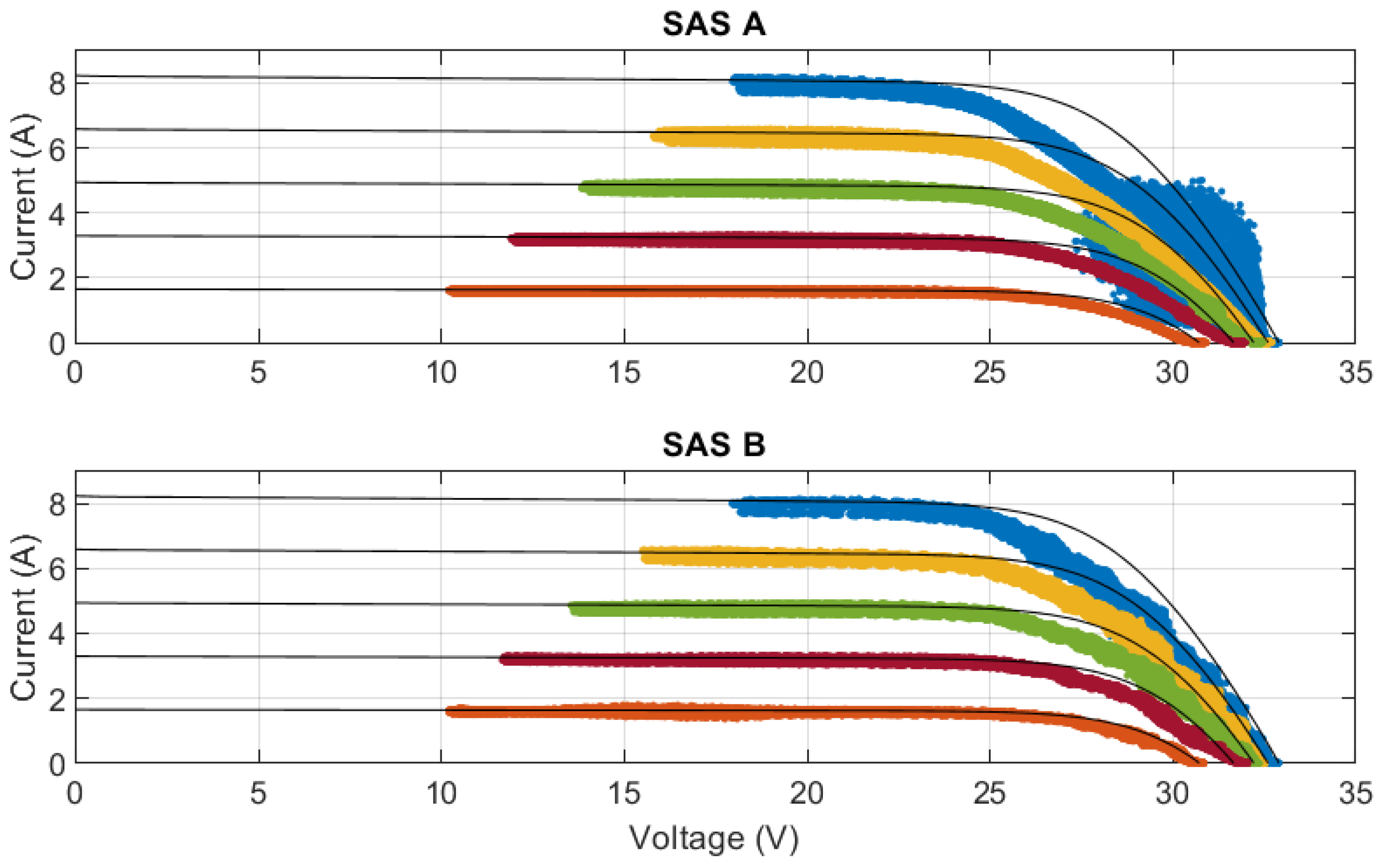
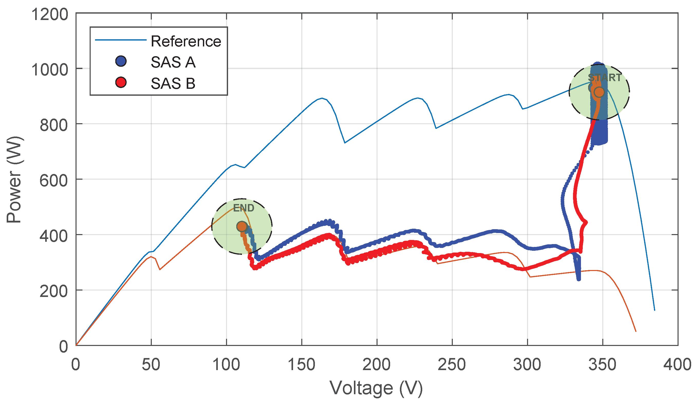
• SAS A is an emulating source equipped with a built-in 16-bit digital control, along with voltage and current measurement circuits. According to the manufacturer, this source is particularly suitable for real-time analysis of maximum power point tracking (MPPT) and for the monitoring of inverter tracking. However, this source does not allow the user to modify the internal control gains. The results obtained with SAS A are graphically represented in blue in the following sections of this work.
• SAS B is a fully programmable emulating source. Its dynamics are determined by the control gains imposed by the user in the graphical supervision interface, allowing for the digital adjustment of properties such as voltage, current, and power. Additionally, this source offers adjustable simulation of internal resistance. The multiprocessing architecture of SAS B enables not only the combination of different control profiles but also real-time data processing. The results obtained with SAS B are graphically represented in red in the following sections of this work.

In the context of controlling the SAS, a different approach is adopted for each of them. Since SAS A does not allow the user to change the gains of its control loop, the factory parameters were maintained during the analyses conducted in this work. However, for SAS B, modifications were made to the current control-loop gains, setting the proportional gain to 50 and the integral gain to 5. These changes were made to enhance the performance of the SAS and obtain more precise and reliable results, as well as to enable deeper evaluations of the source’s behavior.

It is important to note that both commercial SAS models (SAS A and SAS B) have general specifications, as shown in

Table 1. Comparison of evaluated SASs.

Parameter	SAS A	SAS B
Power	0–5 kW	0–10 kW
Current	0–8.5 A	0–13 A
Maximum output voltage	600 V	1000 V
Curve storage	100 *	1000
Point capacity	128	64
Voltage rms ripple	0.11% $FS$ **	0.40% $FS$ **
Peak voltage noise	1.50 V	1.50 V

* Volatile memory. ** Full scale ($FS$).

, which are compatible with experimental applications in research laboratories. These specifications provide important information on the characteristics and features of the SASs.

4. Equipment and Settings Used to Evaluate Emulating Sources

In order to ensure the execution of experiments, proper structuring of the instruments and experimental setup to be used is indispensable. For this purpose, two components were employed to assess the performance of the sources, namely an RC load and a buck–boost converter. These two components are briefly described below.

4.1. Configuration 1: RC Load

This configuration was used to evaluate the response time of the SAS control systems in order to characterize the dynamic behavior of the sources. To do this, this configuration consists of a set of resistors and capacitors connected to the sources in question, as illustrated in Figure 4. Thus, by applying different load steps with known time constants ($\tau$), it is possible to estimate the response time of the emulation source. The resistance of the resistive load, varied from 2.666 $\Omega$ to 8 $\Omega$, while that of the capacitive load varied from 4.7 mF to 47 mF.

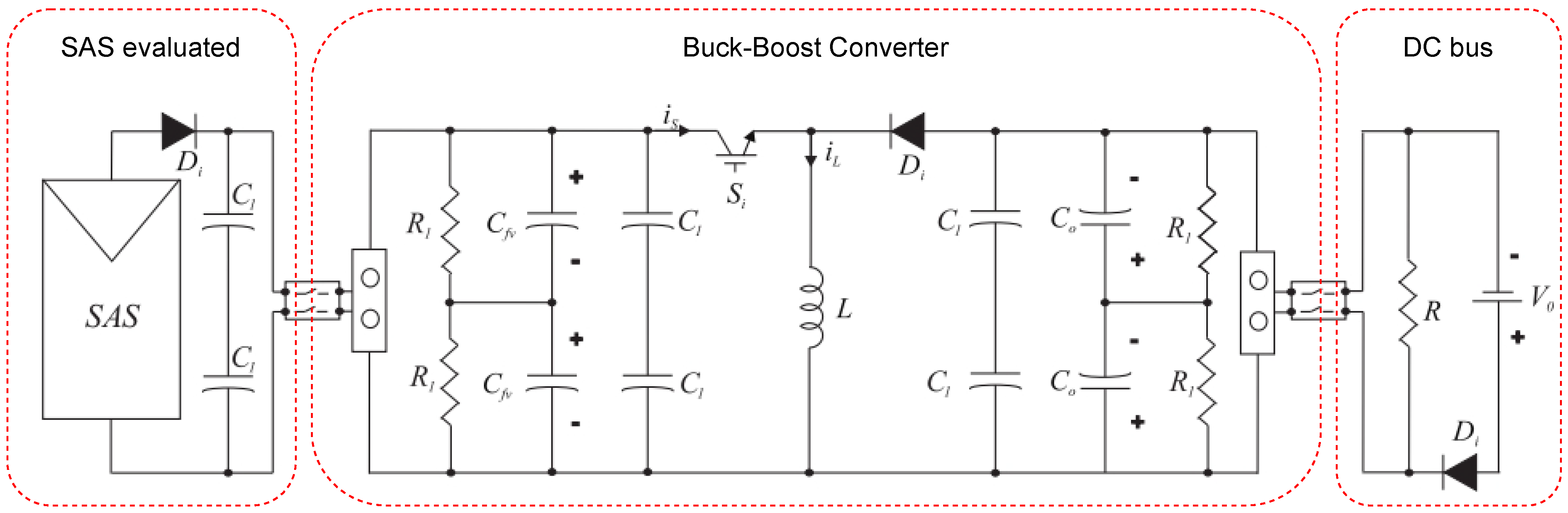
4.2. Configuration 2: Buck–Boost Converter

DC–DC converters can have their duty cycle controlled when connected to a PV module in order to sweep the voltage at the module terminals, ranging from 0 V to $V_{oc}$. By doing this, through voltage and current measurement at the converter input, it becomes possible to generate the I–V curve that characterizes the PV module for the considered irradiance and temperature conditions. In other words, as the duty cycle takes on new values, the PV module interprets the converter to be acting as a resistive load, and for each value, it is assigned a voltage and current [25].

Opting for a DC converter instead of a static load, such as a resistor that only observes a single operating point, makes it feasible to perform I–V curve sweeps. However, it is essential to emphasize that this specific capability is present exclusively in buck–boost converter topologies. The configuration of the buck converter does not allow points close to the short-circuit current ($I_{sc}$) to be obtained, whereas converters with boost characteristics cannot reach points close to the open-circuit voltage ($V_{oc}$) [25].

Figure 5 presents a diagram of the experimental prototype used in the laboratory. In this diagram, the buck–boost converter is configured as the first stage of a two-stage photovoltaic (PV) inverter. Its role is to connect the PV module to the DC bus, enabling the conversion of electrical energy. For emulation source analysis, the PV module in this setup can be emulated by both SAS A and SAS B. In the experimental arrangement, the DC bus is also powered by a DC source, which can, similarly, be SAS A or SAS B. However, as these sources are typically unidirectional, a resistor is added to the DC bus to ensure that the energy generated by the PV module is adequately consumed. Additionally, diodes are placed near the emulating SAS and the source that sets the DC bus voltage to ensure that these devices do not absorb unwanted energy.

This configuration allows for the testing of the emulation of different voltage levels, enabling the evaluation of different types of PV arrays.

Table 2. Specifications of the buck–boost converter.

Parameter	Description	Value
$P_o$	Maximum output power	4000 W
$V_{fv}$	Maximum input voltage	500 V
$V_o$	Maximum output voltage	500 V
$\Delta I_{fv}$	Input current ripple	0.2%
$\Delta I_o$	Output current ripple	0.04%
$f_{sw}$	Switching frequency	20 kHz

lists the specifications of the buck–boost converter, and

Table 3. Specifications of the components of the buck–boost converter.

Parameter	Description	Value
L	Inductance	6 mH
$I_l$	Maximum current through inductor	25 A
$C_{fv}$	Electrolytic capacitors (input)	470 μF
$C_o$	Electrolytic capacitors (output)	330 μF
$C_1$ to $C_4$	Polyester capacitors (high-frequency decoupling)	4.7 μF
$R_1$ to $R_4$	Bus discharge resistors	20 k$\Omega$

describes the values of the components used to construct this converter.

Another important aspect to be discussed is the choice of the load parameters ($R_o$) and the DC bus voltage ($V_o$), both of which are shown in Figure 5. In the following section, which details the conducted experiments and discusses the obtained results, configuration 2, which uses the buck–boost converter, is addressed. In this configuration, two arrangements of photovoltaic modules emulated by the SAS are analyzed, representing different scenarios with varying power ratings. $R_o$ and $V_o$ values are selected to ensure that the system, composed of the converter and the source, operates over the widest possible range, covering all the irradiance levels considered during the experiments.

5. Results

In this section, the main results obtained from the experiments conducted to analyze the steady-state and dynamic behavior of the emulator sources are presented. Based on these results, a brief discussion on the performance of the evaluated sources is conducted.

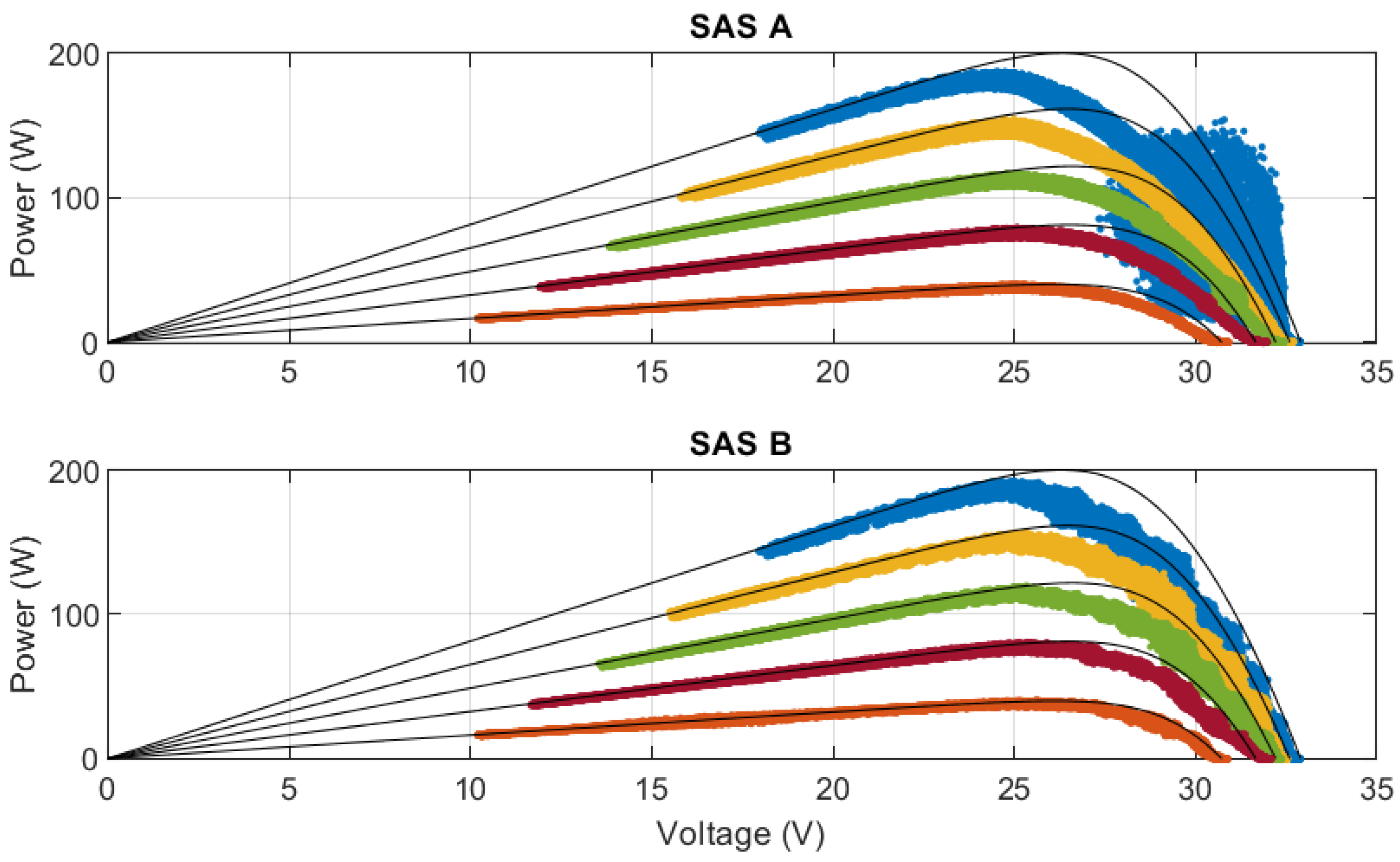
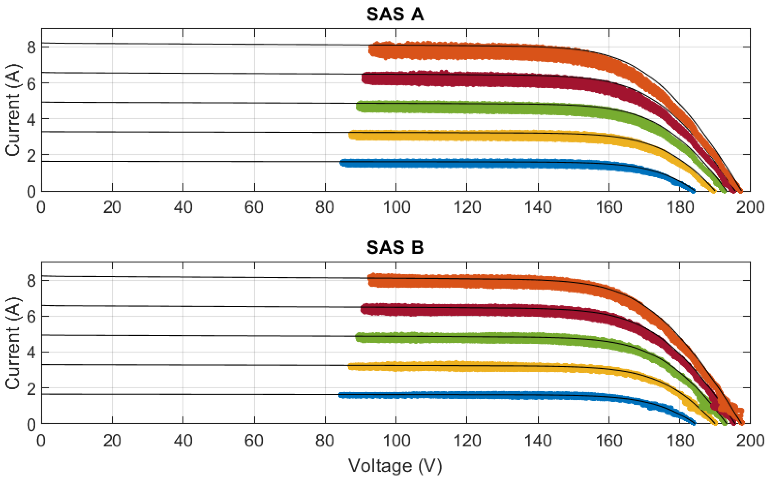
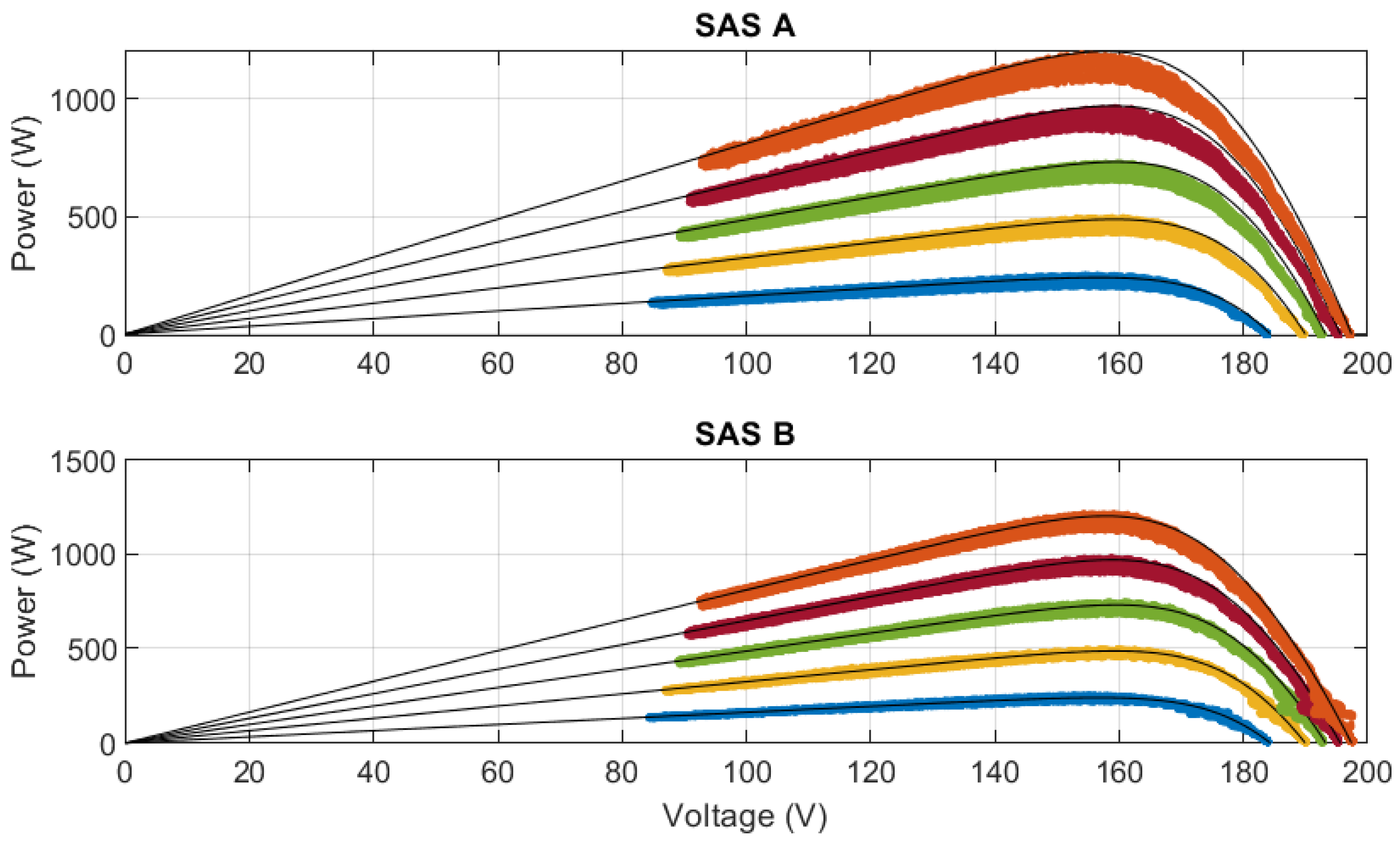
5.1. Steady-State Behavior of SAS

In order to investigate the steady-state behavior of the sources, reference curves were obtained using MATLAB/Simulink software through the PV Array block, which provides a large library of modules. The module chosen for this study is Kyocera KC200GT (monocrystalline silicon technology), and the reference curves were obtained by keeping the temperature fixed at 25 °C and considering five different irradiance levels, namely 200, 400, 600, 800, and 1000 W/m², both for a single module and for six modules in series.

In the simulation conducted to obtain the reference curves, a controlled voltage source was connected to the terminals of the PV array, varying the voltage from 0 to $V_{oc}$ and resulting in a current from $I_{sc}$ to 0. This way, it was possible to obtain the reference curve of the chosen module for a certain irradiance and number of modules. The evaluated points of the curve are linearly spaced to fill the lookup table that each of the sources supports.

The experiments conducted to analyze the steady-state behavior consist of obtaining the I–V and PV curves using a buck–boost converter. The curves obtained during these procedures were evaluated using two widely used error criteria to assess the performance of I–V curves, where the quantity of measured points is denoted as $N_{points}$. The error criteria are the Normalized Mean Absolute Power Error (NMAPE) [26] and the Normalized Root Mean Square Error (NRMSE) [26].

The NMAPE aims to standardize errors in power, allowing the comparison of two or more PV curves of PV modules. NMAPE is calculated using the following formula:

$$NMAPE={\displaystyle \frac{{\sum }_{j=1}^{N_{points}}|P_{ref}-P_{mea}|}{N_{points}·P_{mp}}}·100\%,$$

(1)

where $P_{ref}$ is the power of the reference curves, $P_{mea}$ is the power obtained from the measurements, $N_{points}$ is the number of points present in the analyzed PV curve, and $P_{mp}$ is the maximum power of the reference curve.

$$NRMSE={\displaystyle \frac{\sqrt{\frac{{\sum }_{j=1}^{N_{points}}{(I_{ref}-I_{mea})}^2}{N_{points}}}}{I_{sc}}}·100\%,$$

(2)

where $I_{ref}$ is the current of the reference curves, $I_{mea}$ is the current obtained from the measurements, and $I_{sc}$ is the maximum current of the reference curve.

5.1.1. Results of SASs in Measurements with the Buck–Boost Converter Duty Cycle Varied Linearly

The procedure involved obtaining the I–V and PV curves using the buck–boost converter shown in Figure 5. During this procedure, the duty cycle of the buck–boost converter was varied linearly from 0 to 0.7, then from 0.7 back to 0. Each sweep was performed at 10 s intervals, totaling 20 s per sweep, with current and voltage measured throughout the entire variation. This procedure was repeated five times for each curve, resulting in a total measurement time of 100 s per test. This repetition aimed to gather more data and assess the repeatability of the measurements over time.

It is important to note that the performance of the buck–boost converter does not affect the characteristics highlighted in the results of this evaluation. The results were obtained by exploring various operating points once the converter had reached a steady state. Therefore, the dynamic characteristics of the converter do not impact the evaluation results.

Another important detail to consider is the choice of load, R, and the DC bus voltage, $V_o$, both indicated in Figure 5. When emulating a single module, a load of 6 $\Omega$ and a DC bus voltage of 20 V were used. For the configuration of six modules, a load of 36 $\Omega$ and a voltage of 200 V were employed. These choices ensure that the system, comprising the converter and the source, can operate across the entire range of possible operating conditions (duty cycle between 0 and 0.7), thus covering all evaluated irradiance levels.

The converter successfully performed measurements for all proposed reference configurations, including both a single module and a series of six photovoltaic modules. This allowed for the evaluation of the paths taken in the I–V and PV curves to verify if the source operates along the reference curve.

The results of the single-module measurement, using the linear variation of the duty cycle of the buck–boost converter, are graphically represented in Figure 6 and Figure 7, showing the I–V and PV curves, respectively. It is observed that for this experimental result, a higher power level causes SAS A to enter an unstable region and, consequently, deviate from the applied reference in its configuration. Additionally, it is noted that the sources do not perform well after the knee of the curves, especially at higher currents, as the control system operates to emulate modules in a nonlinear region where the current does not exhibit constant behavior.

The results of the measurement of six modules using the linear variation of the duty cycle of the buck–boost converter are graphically shown in Figure 8 and Figure 9, representing the data of the I–V and PV curves, respectively. From this analysis, it can be observed that for both sources, a higher number of modules in series results in better performance. This is an indication that the control of both sources results in operating points that exhibit better performance.

The NMAPE and NRMSE of the converter measurements for a single module are organized in

Table 4. Evaluation of NMAPE using the buck–boost converter for a single PV module.

Curve	Curve 1 200 W/m2	Curve 2 400 W/m2	Curve 3 600 W/m2	Curve 4 800 W/m2	Curve 5 1 kW/m2
SAS A	7.1760	7.9615	8.1349	9.8986	12.9918
SAS B	4.4700	8.4491	5.5101	9.4378	9.8855

and

Table 5. Evaluation of NRMSE using the buck–boost converter for a single PV module.

Curve	Curve 1 200 W/m2	Curve 2 400 W/m2	Curve 3 600 W/m2	Curve 4 800 W/m2	Curve 5 1 kW/m2
SAS A	0.0027	0.0028	0.0029	0.0035	0.0045
SAS B	0.0017	0.0027	0.0022	0.0029	0.0031

, respectively. For the single-module condition, the average NMAPE for SAS B was $7.55\%$, while for SAS A, it was $9.23\%$, resulting in a difference of $1.68\%$ in favor of SAS B. Regarding NRMSE, SAS B achieved an average value of $0.0025\%$, while SAS A obtained $0.0164\%$, corresponding to a difference of $0.0139\%$ in favor of SAS B.

The NMAPE and NRMSE of the converter measurements for six modules are organized in

Table 6. Evaluation of NMAPE using the buck–boost converter for six PV modules.

Curve	Curve 1 200 W/m2	Curve 2 400 W/m2	Curve 3 600 W/m2	Curve 4 800 W/m2	Curve 5 1 kW/m2
SAS A	5.3046	4.3502	5.0178	3.9010	3.0319
SAS B	1.3504	1.6747	2.1754	1.5903	1.5471

and

Table 7. Evaluation of NRMSE using the buck–boost converter for six PV modules.

Curve	Curve 1 200 W/m2	Curve 2 400 W/m2	Curve 3 600 W/m2	Curve 4 800 W/m2	Curve 5 1 kW/m2
SAS A	0.0016	0.0013	0.0014	0.0012	0.0010
SAS B	0.0006	0.0006	0.0007	0.0006	0.0006

, respectively. For this result, the average NMAPE for SAS B was $1.66\%$, while for SAS A, it was $4.32\%$, resulting in a difference of $2.66\%$ in favor of SAS B. Regarding NRMSE, SAS B achieved an average value of $0.00062\%$, while SAS A obtained $0.0013\%$, corresponding to a difference of $0.00068\%$ in favor of SAS B.

For higher power levels, both sources showed better performance. However, in all conducted tests, SAS B proved to be superior to SAS A.

5.1.2. Steady-State Performance Evaluation

During the analysis of the stationary behavior of the emulator sources, significant errors were observed in the reproduction of the I–V curve when emulating just one PV module, especially near the knee of the curve, where the point of maximum power is located. In addition, the sources found it difficult to represent the nonlinear region between the knee of the I–V curve and the $V_{oc}$ point, where the current is not constant. These results highlight the need to improve the emulator sources in order to guarantee a more faithful and accurate reproduction of the I–V curves at different operating points.

It is essential to emphasize that accurate reproduction of the I–V curve is essential for the use of emulator sources in evaluating the performance and efficiency of MPPT techniques. The errors observed in the knee region and in the nonlinear region of the I–V curve can compromise the accuracy of measurements, mainly affecting model-based MPPT techniques.

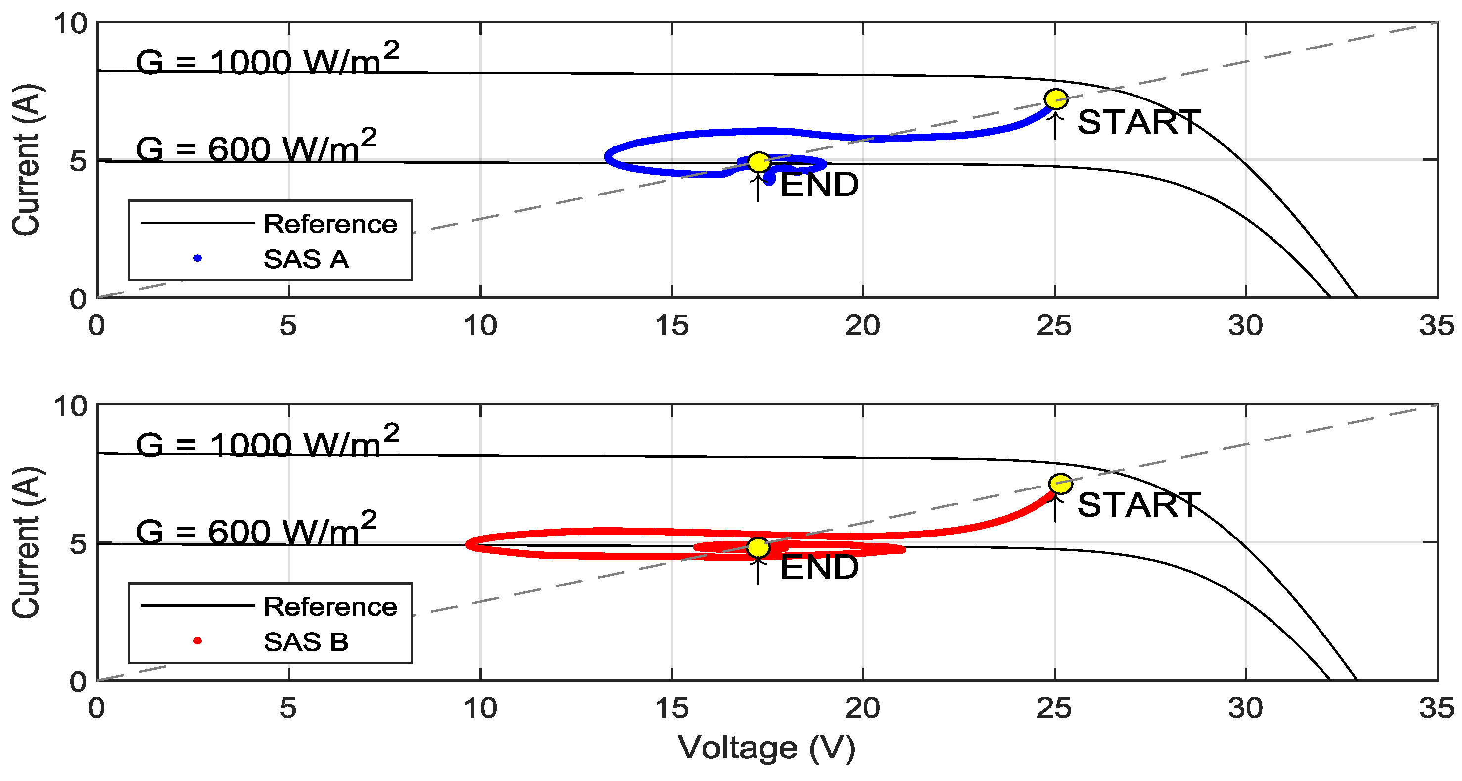
5.2. Transient Behavior of SASs

To evaluate the transient behavior of the emulator sources, three more experiments were carried out. The results of these experiments, together with a discussion of the obtained results, are presented below. It is important to note that the first two described experiments were carried out for the worst-case scenario of the stationary behavior evaluation, i.e., for a single module with an irradiance of 1000 W/m².

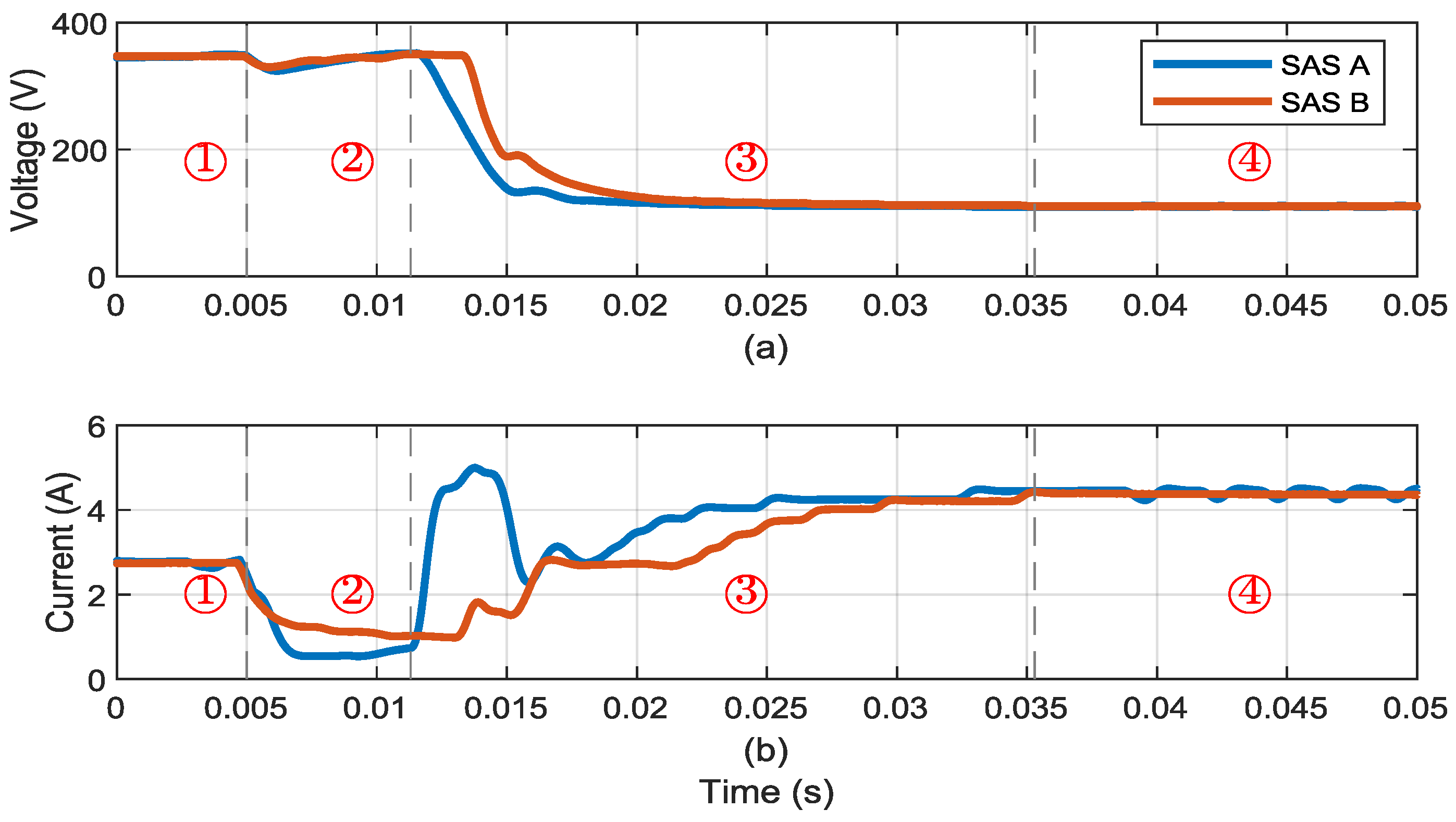
5.2.1. Transient Behavior for Source Connected in Buck–Boost Converter with Fixed Duty Cycle

The aim of this experiment is to observe the transient behavior of the sources during changes in the reference curve, specifically to check whether they follow the reference I–V curve during the transient. The procedure was carried out as illustrated in Figure 5, with the duty cycle of the converter set constantly at 0.7. The transient was then observed while the irradiance levels requested from the sources were varied, starting with a power of 1000 W/m² and decreasing to 600 W/m². The results of the transient with a constant duty cycle and changing reference curves are shown graphically in Figure 10 for the range 1000 W/m² to 600 W/m².

The initial operating point for the selected duty cycle considering an initial reference I–V curve for irradiance of $G=1000$ W/m² is shown in Figure 10. In this figure, it is noticeable that the “start” point does not coincide with the reference I–V curve, as discussed in Section 5.1. When transitioning from the reference I–V curve to the irradiance curve ($G=600$ W/m²), ideally, the system should follow the dashed line in Figure 10, as the converter with a constant duty cycle acts as a resistive load (from the emulated source’s perspective). However, upon observing Figure 10, it is evident that the path taken does not follow the dashed line, forming a circular trajectory around the final operating point (“end” point).

As the graphs shown in Figure 10 are current–voltage graphs, a circular path indicates that the system has underdamped dynamics, resulting in oscillations in both current and voltage around the steady-state operating point. It is therefore hoped that improvements to the source control system can make its response during the curve transition smoother. Furthermore, from this result, it can also be seen that the end point of the sources’ operation coincides with the second reference I–V curve, which was expected, since the “end” point is within the emulator source’s practically constant current operating range (as discussed in Section 5.1).

Finally, from the results of this experiment, it was observed that neither source was able to adequately follow the curve during the change. Both showed very different behavior from what was expected for the emulation of PV modules.

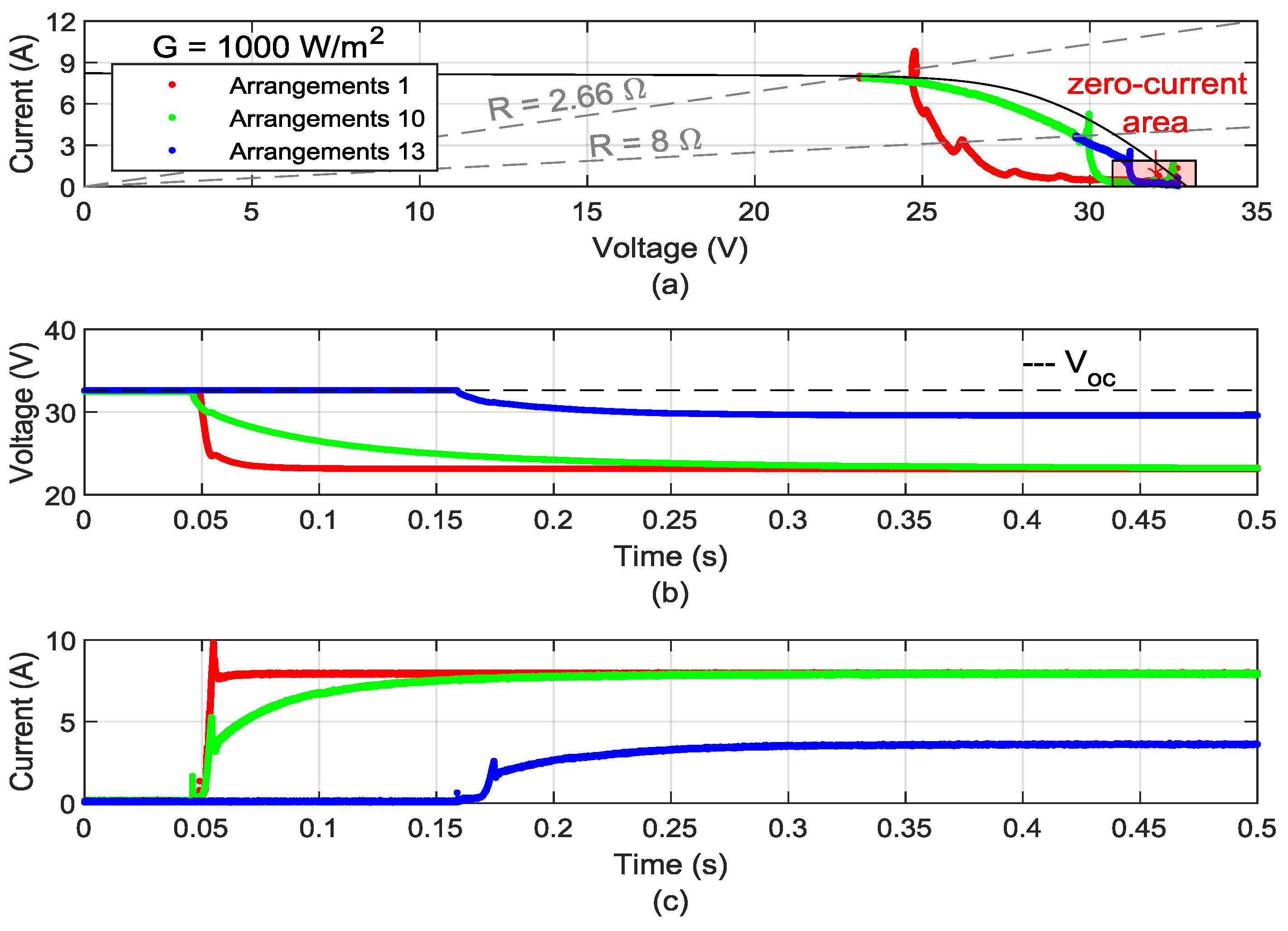
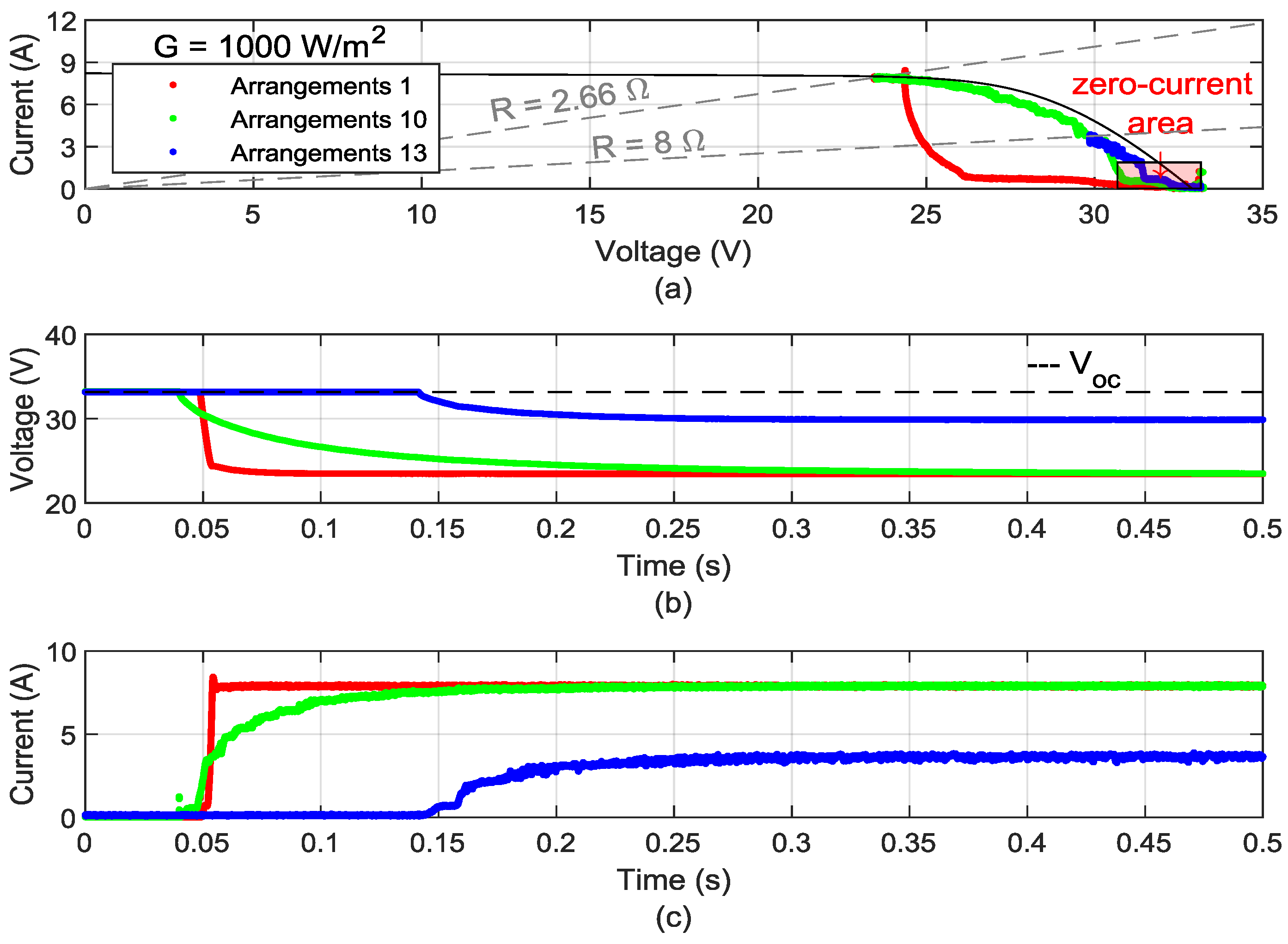
5.2.2. Transient for Source Connected to RC Load

As discussed in Section 5.1, during the evaluation of steady-state behavior, it was observed that the sources had difficulty faithfully reproducing the requested I–V curves, especially when emulating a single PV module. Taking this into account, a second experiment was conducted to rule out the possibility of the sources being unable to keep up with a high current variation occurring after the knee of the I–V curves. These limitations in current and voltage variation rates are referred to in the emulated sources manuals as slew rates.

To rule out the possibility of problems associated with slew rates, it was decided to evaluate the response of the emulated sources to an RC load step. Vy varying the resistance and capacitance of the load, it is possible to adjust the time constant ($\tau$) of the load and make the dynamics slower. This makes it possible to observe the transient behavior of the emulated sources in more detail and verify if they can adequately follow load variations. The specific values of the resistive and capacitive loads used in this evaluation are available in

Table 8. Discrete values of R and C used for configuration 1.

#	Resistance ($\mathbf{\Omega }$)	Capacitance (mF)	Time Constant (ms)
1	2.66	4.70	12.50
2	2.66	9.40	25.06
3	2.66	14.10	37.59
4	2.66	18.80	50.12
5	2.66	23.50	62.65
6	2.66	28.20	75.18
7	2.66	32.90	87.71
8	2.66	37.60	100.24
9	2.66	42.30	112.77
10	2.66	47.00	125.30
11	3.43	47.00	161.11
12	4.80	47.00	225.60
13	8.00	47.00	376.00

.

In this context, as shown in Table 8, it was possible to vary $\tau$, i.e., the time constant of the circuit presented in Figure 4, within a range of values from 12.53 ms to 376 ms Arrangements 1, 2, and 3 presented in Table 8 were used to assess the impact of using RC loads with different time constants connected to the sources. The results depicted in Figure 11 were obtained for SAS A, while Figure 12 represents the use of SAS B.

In this experiment, each emulator source was initially started without being connected to the RC load, configured to operate according to the I–V curve reference of a single PV module with irradiance of $G=1000$ W/m² (black curves in Figure 11a and Figure 12a). Then, each of the three evaluated RC loads was connected to the emulator source terminals. Consequently, the SAS began to operate in a steady state at a point determined by the intersection between the reference I–V curve and the line representing the resistive part of the RC load (dashed line in Figure 11a and Figure 12a).

Ideally, when connecting a load to the emulator source terminals, it is expected that the source stops operating at the initial operating point to operate at the final operating point, following the trajectory defined by the I–V curve. However, analyzing the results presented in Figure 11a and Figure 12a, it can be observed that the voltage starts to decrease before the current starts to increase, resulting in a range of values that makes the trajectory of the change in the operating point pass through a low-current region (indicated by the red shaded area in Figure 11a and Figure 12a) before attempting to follow the I–V curve. Additionally, after this low-current region, significant errors are observed in the knee region and in the nonlinear region of the curve, as mentioned in Section 5.1.

The variations in voltage and current over time for SAS A and SAS B are shown in Figure 11b,c and Figure 12b,c, respectively. By analyzing these curves, it can be observed that initially, the sources respond to voltage variations, then respond to current variations. Furthermore, it is important to note that the response of the sources can be influenced by their voltage and current slew-rate characteristics, which can affect the response time of the sources. Based on these points, it is observed that the larger the time constant of the load (or of the system) connected to the emulator source, the better the source’s ability to follow the trajectory defined by the reference I–V curve. This indicates that slower dynamics may result in a more accurate response from the sources.

Finally, when comparing the results, it is observed that the two sources exhibit similar behaviors. However, SAS A presents a high current overshoot for all values of $\tau$, resulting in a trajectory that passes through points above the reference curve. In addition to the overshoot, even with similar behaviors, SAS B can provide I–V curves closer to the reference curve compared to SAS A.

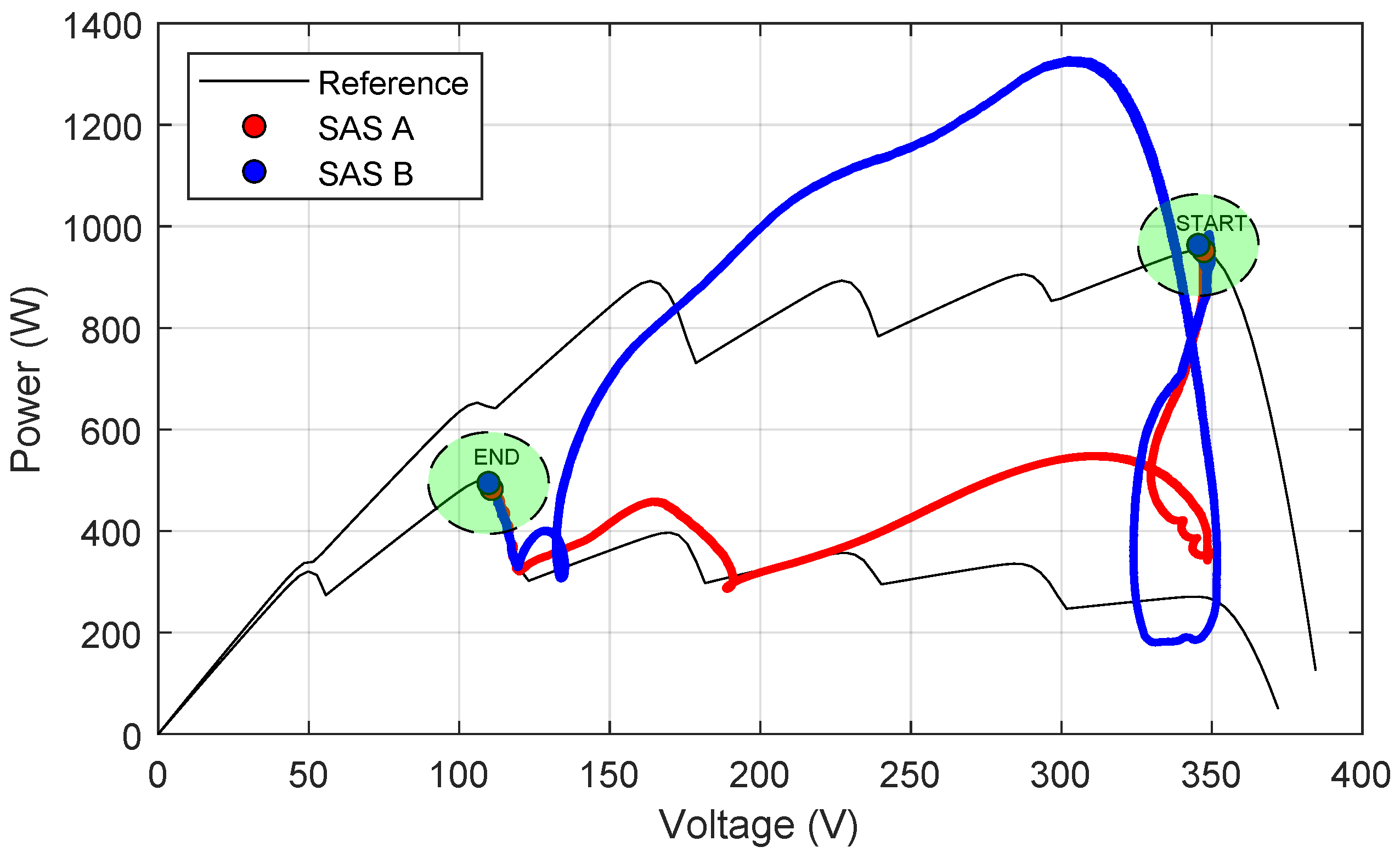
5.2.3. Transient with GMPPT

In the first experiment, the relevance of assessing the impact of varying response times of emulated source controllers was noted, as well as the impact of these sources on the validation of model-based MPPT techniques. It was also deemed important to analyze the behavior of the sources concerning loads that require different response times. Based on these points, a second experiment was conducted with the purpose of investigating these issues.

The second experiment aimed to analyze the transient behavior of the sources during transitions of reference curves. However, shaded curves were used, and the Global Characteristic Curve Maximum Power (GCCMP) technique proposed by Barbosa et al. [12] was also applied. Thus, the experiment involved connecting each source to the buck–boost converter (controlled in a closed loop) and a resistive load. During the measurements, changes were made to the converter controllers, configuring them to be slower. In this context, the following scenarios were evaluated:

• CASE 1—Converter control with regular response time: In this application, the the control loop for the converter input voltage (voltage at the output of the emulated source) was designed that the system had zero error in a steady state, a crossover frequency of 3 kHz, a phase margin of 67.1°, and infinite gain margin. For this purpose, a PI controller with gains of $k_{p1}$ = $0.00012$ and $k_{i1}$ = $0.0318$ was used. The crossover frequency was selected to be ten times lower than the switching frequency, a common practice in static converters with only one control loop.
• CASE 2—Converter control with slow response time: In this application, the gains of the PI controller were decreased to reduce the system’s crossover frequency, making its dynamics slower. For this purpose, a PI controller with gains of $k_{p3}$ = $7.5\times {10}^{-6}$ and $k_{i3}$ = $0.0019875$ was used.

As the buck–boost converter operates in a closed loop, even if there is an abrupt change in the reference I–V curve, the converter control system attempts to regulate the input voltage until the GCCMP algorithm finds a new operating point. This means that during the transient, it is expected that the emulated source transitions from one curve to another while keeping its voltage constant, then tracks the global maximum power point of the new I–V curve. However, the interaction between the buck–boost converter and the emulated source may cause the operating-point transition to not occur as expected, as discussed below.

When using a controller that provides a regular response time in the buck–boost converter (case 1), it is possible to observe four distinct operating ranges in its voltage and current curves (Figure 13). The first range, represented in Figure 13 by ➀, shows the source operating at the global maximum power point of the first I–V curve obtained for $V_{initial}=345.12$ V and $I_{initial}=2.76$ A. With the transition of curves, the SAS begins to behave as indicated in Figure 13 by ➁. In this region, it is observed that the curve change causes a disturbance in the output voltage of the source, but it still remains regulated within the voltage value range ➀, while the current decreases to a new intermediate operating point. At this intermediate point, the GCCMP algorithm seeks the final operating point (global maximum power point of the second I–V curve), resulting in range ➂, which displays the response of the voltage and current of the emulated SAS as it tries to track the global maximum power point. Finally, after a certain time, the curve reaches the final operating point ($V_{final}=108.39$ V and $I_{final}=4.60$ A), as indicated in range ➃.

The voltage and current curves in Figure 13 show the paths taken by the sources, leaving the “start” point and arriving at the “end” point, as shown in Figure 14 (path plotted for PV curve). Figure 14 shows that initially, neither source follows the expected path perfectly. When the curves transition, it becomes clear that the path taken by the source when following the GMPP is above the reference curve, causing the emulator source to produce more power than would be supplied by a real PV module. In fact, for these designed control conditions, the system’s response time cannot be matched by the sources, which ends up degrading the sources’ ability to represent real PV modules.

Although neither source follows the reference curve well (Figure 14), SAS B manages to follow the MPP path more faithfully, while SAS A is too far away from both reference curves. Therefore, according to the results related to GMPP tracking using both sources, the SAS B shows better performance, with more realistic results for comparative analysis of GMPPT techniques but still a considerable error. It is important to consider these results when using emulator fonts to evaluate GMPPT techniques, as differences in font responses can significantly affect the obtained results.

To improve the performance of GMPP tracking, the converter controller parameters were altered in order to obtain a limit operating condition for the evaluated emulator sources (case 2). In this way, the converter’s control system became slower, making the voltage vary more gradually and, consequently, making the current vary more smoothly, ending up respecting the voltage and current slew rates indicated in the sources’ manuals. The results of this evaluation are shown in Figure 15.

Although the results for both sources improved significantly, by slowing down the converter control, the model-based techniques are disadvantaged, as they now spend more time finding the GMPP, establishing an unfair comparison between the algorithms. One solution would be to change the curves/irradiance in a ramp, but the change would not be abrupt, like a step, and the sources are not enabled for this function using the chosen reference curves.

Thus, techniques that use these sources to obtain experimental results calculate parameters (by means of figures of merit) that do not correspond to reality, rewarding techniques that generate a large $dv/dt$ and, therefore, making the simulation results more faithful.

5.2.4. Evaluation of Transient Results

During the analysis of transient behavior conducted in Section 5.2, it was found that neither of the evaluated sources was able to adequately follow the reference curves during the change. Both exhibited behaviors very different from what is expected from PV modules. The control systems of the emulating sources, along with their slew-rate limitations, ended up restricting the ideal operation of the sources during transients.

When evaluating the performance of the sources alongside a closed-loop controlled static converter and with a model-based MPPT algorithm, even larger errors were observed. In fact, due to the inability to correctly represent the curve transition, these sources proved inadequate for evaluation of transient characteristics of this class of MPPT algorithms, since the main benefit of this class of algorithms is their ability to quickly identify the maximum power point of the new reference I–V curve after a transition and transition to that point correctly. For this class of algorithms, an evaluation with mathematical software simulation or application on real PV modules is more appropriate.

The presented results corroborate preliminary observations made by other authors using SASs [27,28]. Although these studies mentioned operational issues, they did not investigate these problems as thoroughly as reported in this article. A notable example identified in the literature is that in aerospace applications, commercial SAS systems do not meet the rapid dynamics required for such applications. As a result, many researchers have developed their own SASs to overcome the dynamic limitations of commercial SAS systems [29,30,31].

6. Conclusions

This article presents a comparative analysis of two commercial SASs, focusing on static and dynamic operation. Several experiments were conducted to investigate the reliability of the I–V curves generated by the sources in relation to real PV modules, the response time of the source control systems, and their behavior both in steady state and during reference-curve transitions.

After thorough analyses, we found the following:

• Regarding static analysis, the analyzed SAS showed inaccuracies in the knee region and in the nonlinear region of the I–V curve, especially when configured to emulate only one module. However, it was observed that increasing the number of modules tended to significantly reduce inaccuracies.
• Regarding dynamic analysis, the analyzed SASs faced difficulties in following the reference curves during transitions. Their dynamic characteristics (resulting from the control system) and their slew-rate limitations ended up generating behaviors divergent from what is expected for PV modules. This limitation is especially critical when evaluating model-based MPPT algorithms, since the ability to quickly identify the maximum power point after a change in the I–V curve is crucial for the efficiency of this class of algorithms.

Thus, it can be concluded that the use of SASs, especially those studied in this article, to evaluate the performance of MPPT techniques requires attention to their limitations and inaccuracies. To obtain more precise and reliable results, especially when analyzing model-based MPPT algorithms, other approaches, such as simulations using mathematical software or application on real PV modules, may be more suitable.

References

1. Azharuddin, S.M.; Vysakh, M.; Thakur, H.V.; Nishant, B.; Babu, T.S.; Muralidhar, K.; Paul, D.; Jacob, B.; Balasubramanian, K.; Rajasekar, N. A Near Accurate Solar PV Emulator Using dSPACE Controller for Real-time Control. Energy Procedia 2014, 61, 2640–2648. [Google Scholar] [CrossRef]
2. Alghamdi, H.; Alviz-Meza, A. Techno-Environmental Evaluation and Optimization of a Hybrid System: Application of Numerical Simulation and Gray Wolf Algorithm in Saudi Arabia. Sustainability 2023, 15, 3284. [Google Scholar] [CrossRef]
3. Yilmaz, M. Comparative Analysis of Hybrid Maximum Power Point Tracking Algorithms Using Voltage Scanning and Perturb and Observe Methods for Photovoltaic Systems under Partial Shading Conditions. Sustainability 2024, 16, 4199. [Google Scholar] [CrossRef]
4. Subbulakshmy, R.; Palanisamy, R.; Alshahrani, S.; Saleel, C.A. Implementation of Non-Isolated High Gain Interleaved DC-DC Converter for Fuel Cell Electric Vehicle Using ANN-Based MPPT Controller. Sustainability 2024, 16, 1335. [Google Scholar] [CrossRef]
5. Farhangi, S.; Nazer, A.; Moradi, G.R.; Asadi, E. Improved Performance of Solar Array Simulator Based on Constant Voltage/Constant Current Full-Bridge Converter. In Proceedings of the 2020 11th Power Electronics, Drive Systems, and Technologies Conference (PEDSTC), Tehran, Iran, 4–6 February 2020; pp. 1–5. [Google Scholar]
6. Nagadurga, T.; Narasimham, P.V.R.L.; Vakula, V.S. Global Maximum Power Point Tracking of Solar Photovoltaic Strings under Partial Shading Conditions Using Cat Swarm Optimization Technique. Sustainability 2021, 13, 11106. [Google Scholar] [CrossRef]
7. Ram, J.P.; Manghani, H.; Pillai, D.S.; Babu, T.S.; Miyatake, M.; Rajasekar, N. Analysis on solar PV emulators: A review. Renew. Sustain. Energy Rev. 2018, 81, 149–160. [Google Scholar] [CrossRef]
8. Dawahdeh, A.; Sharadga, H.; Kumar, S. Novel MPPT Controller Augmented with Neural Network for Use with Photovoltaic Systems Experiencing Rapid Solar Radiation Changes. Sustainability 2024, 16, 1021. [Google Scholar] [CrossRef]
9. Cupertino, A.F.; Santos, G.Y.; Cardoso, E.N.; Pereira, H.A.; Mendes, V.F. Modeling and design of a flexible solar array simulator topology. In Proceedings of the 2015 IEEE 13th Brazilian Power Electronics Conference and 1st Southern Power Electronics Conference (COBEP/SPEC), Fortaleza, Brazil, 29 November–2 December 2015; pp. 1–6. [Google Scholar]
10. Punitha, K.; Rahman, A.; Radhamani, A.S.; Nuvvula, R.S.S.; Shezan, S.A.; Ahammed, S.R.; Kumar, P.P.; Ishraque, M.F. An Optimization Algorithm for Embedded Raspberry Pi Pico Controllers for Solar Tree Systems. Sustainability 2024, 16, 3788. [Google Scholar] [CrossRef]
11. Ayop, R.; Tan, C.W. A comprehensive review on photovoltaic emulator. Renew. Sustain. Energy Rev. 2017, 80, 430–452. [Google Scholar] [CrossRef]
12. Barbosa, E.J.; Cavalcanti, M.C.; de Souza Azevedo, G.M.; Barbosa, E.A.; Bradaschia, F.; Limongi, L.R. Global Hybrid Maximum Power Point Tracking for PV Modules Based on a Double-Diode Model. IEEE Access 2021, 9, 158440–158455. [Google Scholar] [CrossRef]
13. Ye, S.P.; Liu, Y.H.; Pai, H.Y.; Sangwongwanich, A.; Blaabjerg, F. A Novel ANN-Based GMPPT Method for PV Systems under Complex Partial Shading Conditions. IEEE Trans. Sustain. Energy 2024, 15, 328–338. [Google Scholar] [CrossRef]
14. Kumaresan, A.; Tafti, H.D.; Beniwal, N.; Gorla, N.B.Y.; Farivar, G.G.; Pou, J.; Konstantinou, G. Improved Secant-Based Global Flexible Power Point Tracking in Photovoltaic Systems Under Partial Shading Conditions. IEEE Trans. Power Electron. 2023, 38, 10383–10395. [Google Scholar] [CrossRef]
15. Jassim, B.; Jasim, H. Modelling of a solar array simulator based on multiple DC-DC converters. Int. J. Renew. Energy Res. 2018, 8, 1038–1044. [Google Scholar]
16. Norman, K.; Ren, B.; Zhong, Q.C. Learning-by-Doing: Design and Implementation of a Solar Array Simulator with a SYNDEM Smart Grid Research and Educational Kit. IEEE Power Electron. Mag. 2024, 11, 47–54. [Google Scholar] [CrossRef]
17. Zhou, H.; Sun, Y.; Zhang, M.; Ni, Y.; Zhang, F.; Young Jeong, S.; Huang, T.; Li, X.; Woo, H.Y.; Zhang, J.; et al. Over 18.2% efficiency of layer–by–layer all–polymer solar cells enabled by homoleptic iridium(III) carbene complex as solid additive. Sci. Bull. 2024; in press. [Google Scholar]
18. Xia, H.; Zhang, M.; Wang, H.; Sun, Y.; Li, Z.; Ma, R.; Liu, H.; Dela Peña, T.A.; Chandran, H.T.; Li, M.; et al. Leveraging Compatible Iridium(III) Complexes to Boost Performance of Green Solvent-Processed Non-Fullerene Organic Solar Cells. Adv. Funct. Mater. 2024, 2411058. [Google Scholar] [CrossRef]
19. Seo, Y.T.; Park, J.Y.; Choi, S.J. A rapid I-V curve generation for PV model-based solar array simulators. In Proceedings of the 2016 IEEE Energy Conversion Congress and Exposition (ECCE), Milwaukee, WI, USA, 18–22 September 2016; pp. 1–5. [Google Scholar]
20. Coelho, R.F.; Concer, F.; Martins, D.C. A Study of the Basic DC-DC Converters Applied in Maximum Power Point Tracking. In Proceedings of the 2009 Brazilian Power Electronics Conference, Bonito-Mato Grosso do Sul, Brazil, 27 September–1 October 2009; pp. 673–678. [Google Scholar]
21. Chroma. Solar Array Simulation Soft Panel. Available online: https://www.chromausa.com/62000h-s-solar-array-simulation-video/ (accessed on 23 July 2024).
22. Ecosense. Solar PV Emulator System (SPVE). Available online: https://www.ecosenseworld.com/sites/default/files/spve.pdf (accessed on 23 July 2024).
23. Technologies, K. Keysight E4360 Modular Solar Array Simulators. Available online: https://www.axiomtest.com/documents/models/Keysight%20N8937APV%20DATASHEET.pdf (accessed on 23 July 2024).
24. Regatron. SASControl Software Solar Array Simulation Program Manual. Available online: https://ohmini.com.br/downloads/catalogos/simulador-fotovoltaico/Catalogo-SASControl.pdf (accessed on 23 July 2024).
25. Treter, M.E.; Michels, L. Métodos de aquisição experimental de curvas I-V de arranjos fotovoltaicos: Uma revisão. In Proceedings of the 1th Seminar on Power Electronics and Control-SEPOC, Santa Maria, Brazil, 21–24 October 2018. [Google Scholar]
26. Cavalcante, V.M.; Fernandes, T.A.; Freitas, R.A.; Bradaschia, F.; Cavalcanti, M.C.; Limongi, L.R. A Global Nonlinear Model for Photovoltaic Modules Based on 3-D Surface Fitting. IEEE J. Photovolt. 2024, 1–9. [Google Scholar] [CrossRef]
27. Jin, S.; Zhang, D.; Bao, Z.; Liu, X. High Dynamic Performance Solar Array Simulator Based on a SiC MOSFET Linear Power Stage. IEEE Trans. Power Electron. 2018, 33, 1682–1695. [Google Scholar] [CrossRef]
28. Cupertino, A.F.; Pereira, H.A.; Mendes, V.F. Modeling, Design and Control of a Solar Array Simulator Based on Two-Stage Converters. J. Control. Autom. Electr. Syst. 2017, 28, 585–596. [Google Scholar] [CrossRef]
29. Jin, S.; Zhang, D.; Wang, C. UI-RI Hybrid Lookup Table Method with High Linearity and High-Speed Convergence Performance for FPGA-Based Space Solar Array Simulator. IEEE Trans. Power Electron. 2018, 33, 7178–7192. [Google Scholar] [CrossRef]
30. Orts, C.; Garrigós, A.; Marroquí, D.; Franke, A. Sequential Switching Shunt Regulation Using DC Transformers for Solar Array Power Processing in High Voltage Satellites. IEEE Trans. Aerosp. Electron. Syst. 2024, 60, 421–429. [Google Scholar] [CrossRef]
31. Jin, S.; Zhang, D.; Wang, C.; Gu, Y. Optimized Design of Space Solar Array Simulator with Novel Three-Port Linear Power Composite Transistor Based on Multiple Cascaded SiC-JFETs. IEEE Trans. Ind. Electron. 2018, 65, 4691–4701. [Google Scholar] [CrossRef]
Figure 1. Examples of PV curve-generating elements for inverter and MPPT algorithm testing: (a) PV module; (b) SAS.
Sustainability 16 06932 g001
Figure 2. Standard structure of an SAS.
Sustainability 16 06932 g002
Figure 3. Graphic interfaces of SAS systems: (a) Chroma [21]; (b) Ecosense [22]; (c) Keysight [23]; (d) Regatron [24].
Sustainability 16 06932 g003
Figure 4. Configuration 1—Schematic for the experiments related to the behavior of the sources (SAS + RC load).
Sustainability 16 06932 g004
Figure 5. Configuration 2—Schematic of the experiments related to the behavior of the sources (SAS + buck–boost converter).
Sustainability 16 06932 g005
Figure 6. Evaluation of the steady-state behavior of SASs: obtaining I–V curves with the buck–boost converter for the configuration of a module with irradiance ranging from 200 to 1000 W/m2.
Sustainability 16 06932 g006
Figure 7. Evaluation of the steady-state behavior of SASs: obtaining PV Curves with the buck–boost converter for the configuration of a module with irradiance ranging from 200 to 1000 W/m2.
Sustainability 16 06932 g007
Figure 8. Evaluation of the steady-state behavior of emulated sources: obtaining I–V Curves with the buck–boost converter for the configuration of six modules with irradiance ranging from 200 to 1000 W/m2.
Sustainability 16 06932 g008
Figure 9. Evaluation of the steady-state behavior of emulated sources: obtaining I–V curves with the buck–boost converter for the configuration of six modules with irradiance ranging from 200 to 1000 W/m2.
Sustainability 16 06932 g009
Figure 10. Behavior of the evaluated sources for a transient in the I–V curve from 1000 to 600 W/m2. Results obtained for sources connected in a fixed duty cycle buck–boost converter.
Sustainability 16 06932 g010
Figure 11. Behavior of SAS A in response to an RC load step, applying loads with different time constants ( τ ): 12.53 ms (configuration 1), 125.30 ms (configuration 10), and 376.00 ms (configuration 13). (a) Path on the I–V curve; (b) voltage variation; (c) current variation.
Sustainability 16 06932 g011
Figure 12. Behavior of SAS B in response to an RC load step, applying loads with different time constants ( τ ): 12.53 ms (configuration 1), 125.30 ms (configuration 10), and 376.00 ms (configuration 13). (a) Path on the I–V curve; (b) voltage variation; (c) current variation.
Sustainability 16 06932 g012
Figure 13. Transient behavior of current and voltage of the evaluated SAS for shaded curves using the GCCMP technique (case 1). (a) voltage variation; (b) current variation.
Sustainability 16 06932 g013
Figure 14. Trajectory followed by the evaluated SAS regarding the PV curves, considering shaded curves and using the GCCMP technique (case 1).
Sustainability 16 06932 g014
Figure 15. Trajectory followed by the evaluated SAS regarding the PV curves, considering shaded curves and using the GCCMP technique (case 2).
Sustainability 16 06932 g015