


Photovoltaic Modeling: A Comprehensive Analysis of the I–V Characteristic Curve


Abstract
1. Introduction
- Provide a comprehensive summary of some of the widely used PV models in literature.
- Evaluate the accuracy of these models at MPP in accordance with the IEC EN 50530 standard.
- Identify limitations in existing photovoltaic (PV) models and propose potential research directions in this field with the aim of advancing toward energy sustainability.
2. Equivalent-Circuit-Based Models
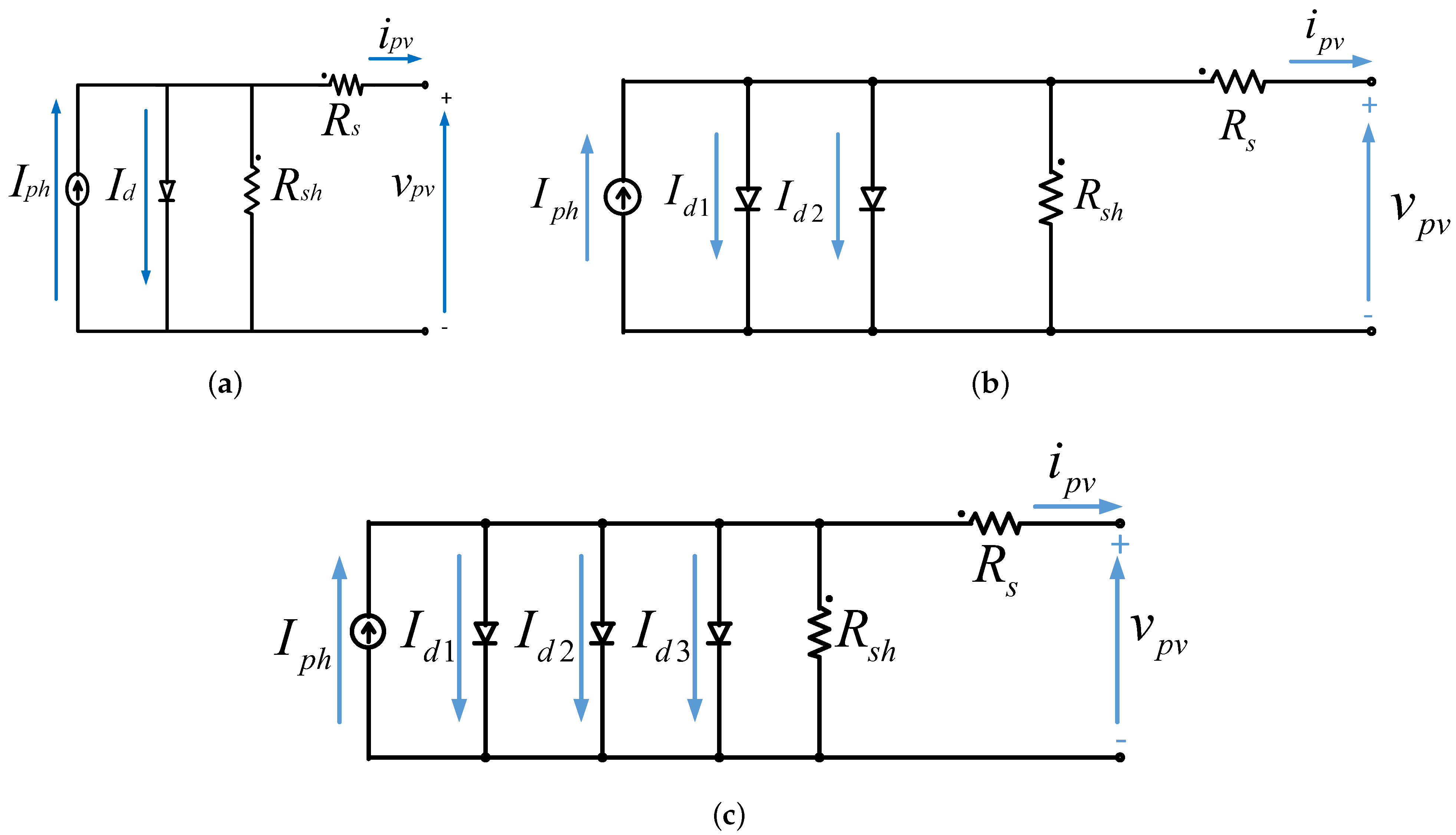
2.1. Single-Diode Model
2.2. Double-Diode Model
2.3. Triple-Diode Model
3. Approximate PV Models
3.1. Approximation Using the Lambert W Function and the Asymptotic Formula
3.2. Other Analytical-Based PVM Equations
4. Empirical-Based PV Models
4.1. Three-Coefficient Model
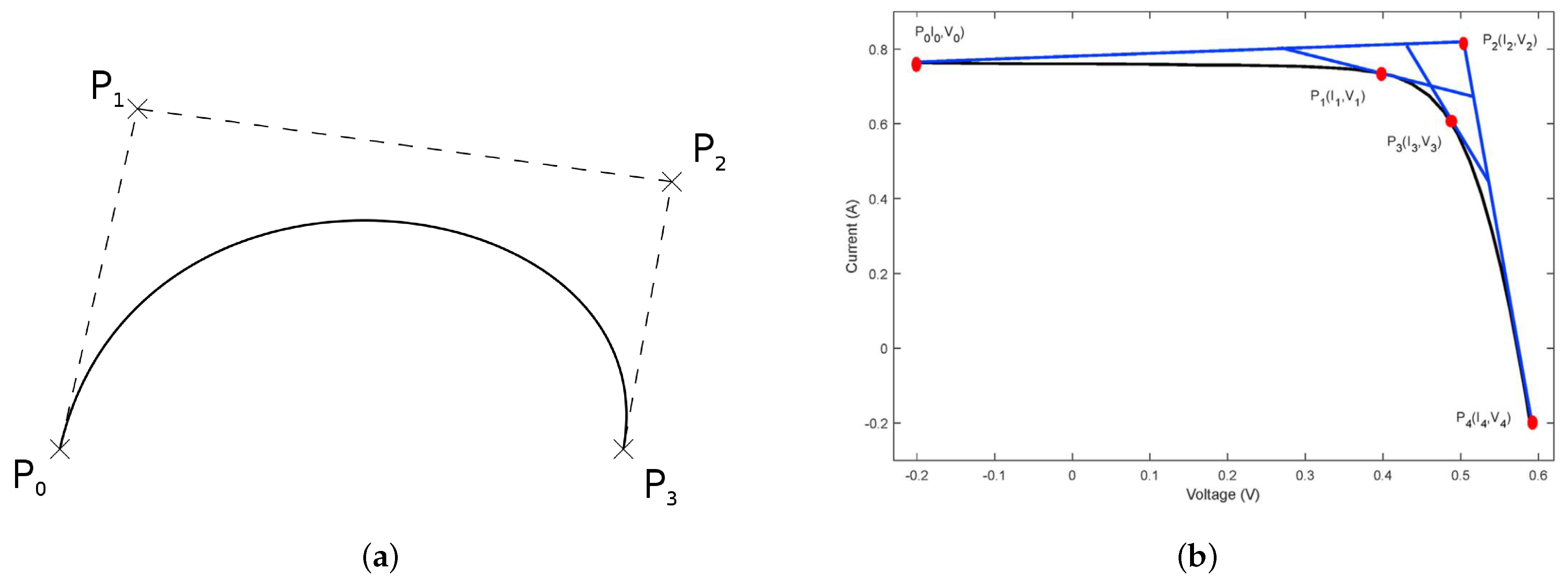
4.2. Bézier Curve-Based Model
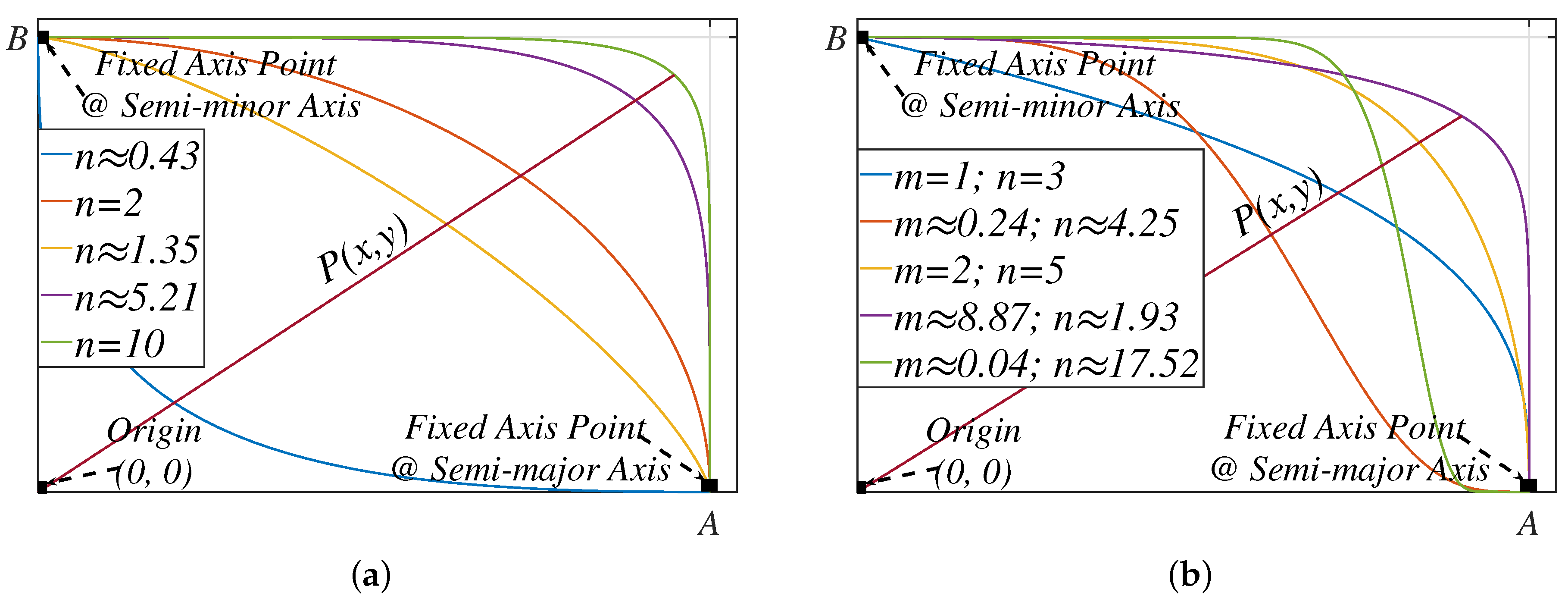
4.3. Superellipse-Based Model
5. Comparative Evaluation and Further Discussion
5.1. Criteria for Evaluating Model Accuracy
5.2. Parameter Convergence
5.3. Accuracy Evaluation Using the IEC EN 50530 Standard
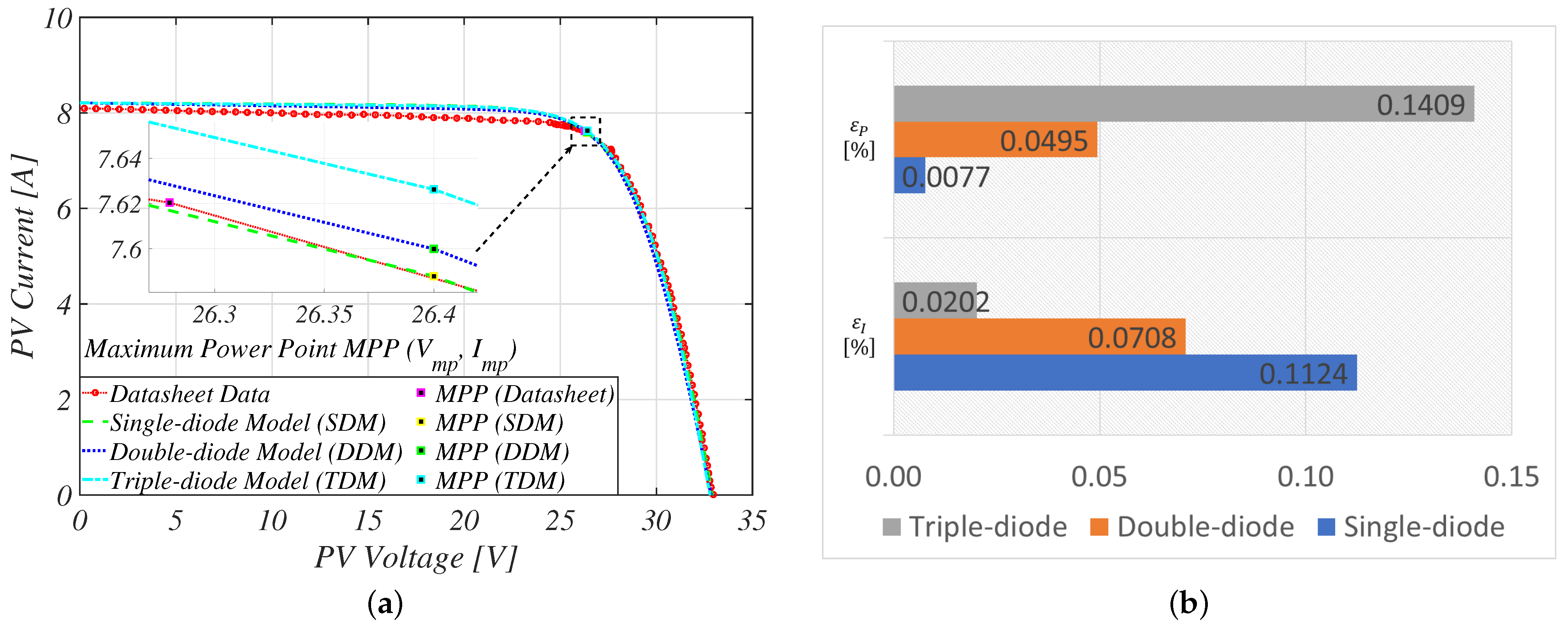
5.3.1. Comparison of the Equivalent-Circuit-Based Models
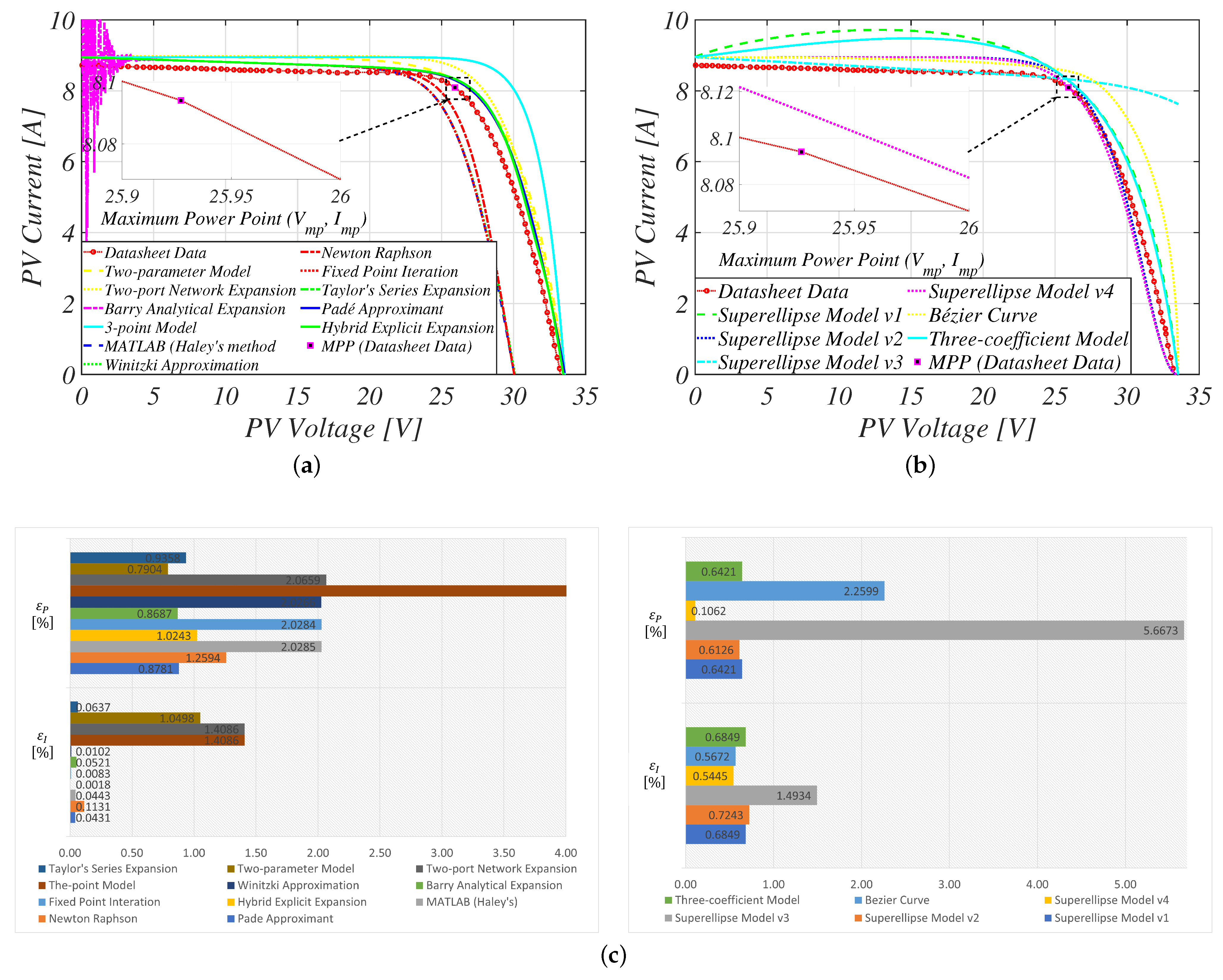
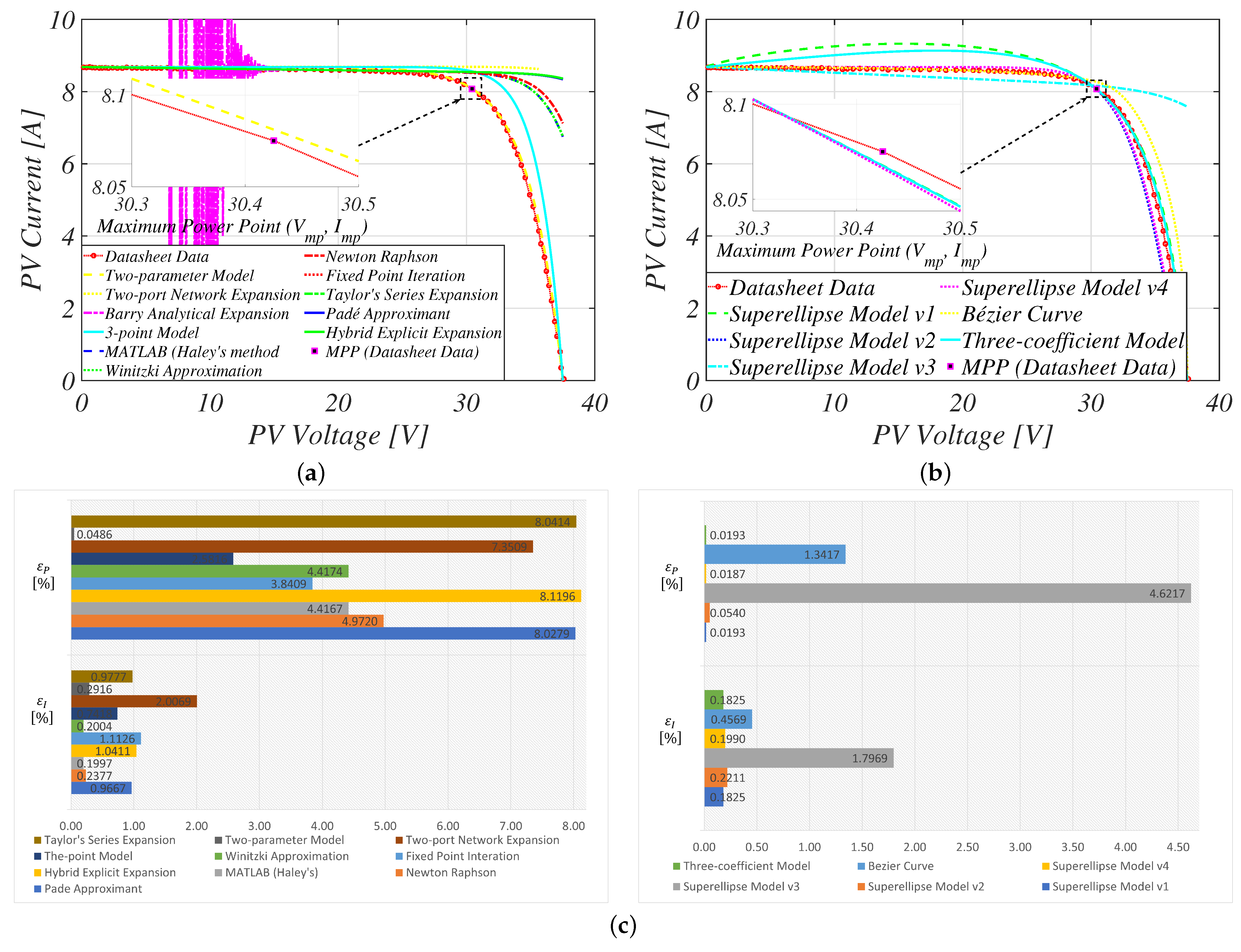
5.3.2. Comparison of the Approximate PV Models
5.3.3. Comparison of the Empirical-Based Models
5.4. Research Trends
- Equivalent-circuit-based PV models: For practitioners with prior experience in both the electrical behavior and conversion principles describing a PV panel, circuit-based models offer a more inclusive representation of the nonlinear characteristics of the I–V curve. However, to improve model accuracy, more research is needed to identify simple and effective techniques for accurately estimating the electrical parameters of PV panels.
- Analytical-based PV models: Since the explicit equations describing these PV models are derivatives from the conventional circuit-based model (single-diode), the model accuracy of the current approximate PVM equations in the literature is still dependent on the basic five electrical parameters. Nonetheless, the novelty and major contributions in this research will always lie in the relative simplification of the equation used for the reconstruction of the I–V curve.
- Empirical-based PV models: One of the main limitations of curve-fitting PV models is that they do not fully consider the specific characteristics of the PV panel. However, these models are very useful because they are relatively simple and easy to use for reconstructing the PV characteristic curve. While many equations could potentially generate a similar shape to the I–V curve, a hybrid model that combines the advantages of both circuit-based and empirical-based models would provide a better understanding of both the static and dynamic characteristics of the PV panel.
6. Conclusions
Author Contributions
Funding
Institutional Review Board Statement
Informed Consent Statement
Data Availability Statement
Conflicts of Interest
Appendix A. IEC EN 50530 Standard—Overall Efficiency of Grid Connected Photovoltaic Inverters

| cSi-Technology | Thin-Film Technology | Tolerance | |
|---|---|---|---|
| 0.95 | 0.98 | ||
| 0.8 | 0.72 | ||
| 0.9 | 0.8 |
References
- Nejat, P.; Jomehzadeh, F.; Taheri, M.M.; Gohari, M.; Majid, M.Z.A. A global review of energy consumption, CO2 emissions and policy in the residential sector (with an overview of the top ten CO2 emitting countries). Renew. Sustain. Energy Rev. 2015, 43, 843–862. [Google Scholar] [CrossRef]
- Metz, B.; Davidson, O.; De Coninck, H.; Loos, M.; Meyer, L. IPCC Special Report on Carbon Dioxide Capture and Storage; Cambridge University Press: Cambridge, UK, 2005. [Google Scholar]
- Bouich, A.; Pradas, I.G.; Khan, M.A.; Khattak, Y.H. Opportunities, Challenges, and Future Prospects of the Solar Cell Market. Sustainability 2023, 15, 15445. [Google Scholar] [CrossRef]
- Afolayan, M.; Olayiwola, T.; Nurudeen, Q.; Ibrahim, O.; Madugu, I. Performance Evaluation of Soiling Mitigation Technique for Solar Panels. Arid. Zone J. Eng. Technol. Environ. 2020, 16, 685–698. [Google Scholar]
- Parida, B.; Iniyan, S.; Goic, R. A review of solar photovoltaic technologies. Renew. Sustain. Energy Rev. 2011, 15, 1625–1636. [Google Scholar] [CrossRef]
- Sampaio, P.G.V.; González, M.O.A. Photovoltaic solar energy: Conceptual framework. Renew. Sustain. Energy Rev. 2017, 74, 590–601. [Google Scholar] [CrossRef]
- Singh, G.K. Solar power generation by PV (photovoltaic) technology: A review. Energy 2013, 53, 1–13. [Google Scholar] [CrossRef]
- Lazaroiu, A.C.; Gmal Osman, M.; Strejoiu, C.V.; Lazaroiu, G. A Comprehensive Overview of Photovoltaic Technologies and Their Efficiency for Climate Neutrality. Sustainability 2023, 15, 16297. [Google Scholar] [CrossRef]
- Mahmood, A.; Irfan, A.; Wang, J.L. Molecular level understanding of the chalcogen atom effect on chalcogen-based polymers through electrostatic potential, non-covalent interactions, excited state behaviour, and radial distribution function. Polym. Chem. 2022, 13, 5993–6001. [Google Scholar] [CrossRef]
- Mahmood, A.; Hu, J.Y.; Xiao, B.; Tang, A.; Wang, X.; Zhou, E. Recent progress in porphyrin-based materials for organic solar cells. J. Mater. Chem. A 2018, 6, 16769–16797. [Google Scholar] [CrossRef]
- Mehboob, M.Y.; Hussain, R.; Adnan, M.; Irshad, Z.; Khalid, M. Impact of π-linker modifications on the photovoltaic performance of rainbow-shaped acceptor molecules for high performance organic solar cell applications. Phys. B Condens. Matter 2022, 625, 413465. [Google Scholar] [CrossRef]
- Khalid, M.; Murtaza, S.; Bano, M.; Shafiq, I.; Jawaria, R.; Ataulapa, A. Role of extended end-capped acceptors in non-fullerene based compounds towards photovoltaic properties. J. Photochem. Photobiol. A Chem. 2024, 448, 115292. [Google Scholar] [CrossRef]
- Tang, J.; Ni, H.; Peng, R.L.; Wang, N.; Zuo, L. A review on energy conversion using hybrid photovoltaic and thermoelectric systems. J. Power Sources 2023, 562, 232785. [Google Scholar] [CrossRef]
- National Renewable Energy Laboratory Interactive Best Research-Cell Efficiency Chart. 2023. Available online: https://www.nrel.gov/pv/interactive-cell-efficiency.html (accessed on 13 December 2023).
- Schultz, O.; Preu, R.; Glunz, S. Silicon solar cells with screenprinted front side metallization exceeding 19% efficiency. In Proceedings of the 22nd European Photovoltaic Solar Energy Conference and Exhibition, Milan, Italy, 3–7 September 2007; Volume 3, p. 7. [Google Scholar]
- Richter, A.; Hermle, M.; Glunz, S.W. Reassessment of the limiting efficiency for crystalline silicon solar cells. IEEE J. Photovoltaics 2013, 3, 1184–1191. [Google Scholar] [CrossRef]
- Yoshikawa, K.; Kawasaki, H.; Yoshida, W.; Irie, T.; Konishi, K.; Nakano, K.; Uto, T.; Adachi, D.; Kanematsu, M.; Uzu, H.; et al. Silicon heterojunction solar cell with interdigitated back contacts for a photoconversion efficiency over 26%. Nat. Energy 2017, 2, 17032. [Google Scholar] [CrossRef]
- Gobichettipalayam Shanmugam, S.K.; Sakthivel, T.S.; Gaftar, B.A.; Iyyappan, P.; Sathyamurthy, R. Modeling and simulation of single-and double-diode PV solar cell model for renewable energy power solution. Environ. Sci. Pollut. Res. 2022, 29, 4414–4430. [Google Scholar] [CrossRef] [PubMed]
- Hernández-López, D.; Oña, E.R.d.; Moreno, M.A.; González-Aguilera, D. SunMap: Towards Unattended Maintenance of Photovoltaic Plants Using Drone Photogrammetry. Drones 2023, 7, 129. [Google Scholar] [CrossRef]
- Nayak, J.; Thalla, H.; Ghosh, A. Efficient maximum power point tracking algorithms for photovoltaic systems with reduced number of sensors. Process. Integr. Optim. Sustain. 2022, 7, 191–213. [Google Scholar] [CrossRef]
- Eiffert, P. Building-Integrated Photovoltaic Designs for Commercial and Institutional Structures: A Sourcebook for Architects; DIANE Publishing: Collingdale, PA, USA, 2000. [Google Scholar]
- Bader, S.; Ma, X.; Oelmann, B. One-diode photovoltaic model parameters at indoor illumination levels—A comparison. Sol. Energy 2019, 180, 707–716. [Google Scholar] [CrossRef]
- Pranith, S.; Bhatti, T. Modeling and parameter extraction methods of PV modules. In Proceedings of the 2015 International Conference on Recent Developments in Control, Automation and Power Engineering (RDCAPE), Noida, India, 12–13 March 2015; pp. 72–76. [Google Scholar]
- Vinod; Kumar, R.; Singh, S.K. Solar photovoltaic modeling and simulation: As a renewable energy solution. Energy Rep. 2018, 4, 701–712. [Google Scholar] [CrossRef]
- Pendem, S.R.; Mikkili, S. Modeling, simulation and performance analysis of solar PV array configurations (Series, Series–Parallel and Honey-Comb) to extract maximum power under Partial Shading Conditions. Energy Rep. 2018, 4, 274–287. [Google Scholar] [CrossRef]
- Pongratananukul, N.; Kasparis, T. Tool for automated simulation of solar arrays using general-purpose simulators. In Proceedings of the 2004 IEEE Workshop on Computers in Power Electronics, Urbana, IL, USA, 15–18 August 2004; pp. 10–14. [Google Scholar]
- Chin, V.J.; Salam, Z.; Ishaque, K. Cell modelling and model parameters estimation techniques for photovoltaic simulator application: A review. Appl. Energy 2015, 154, 500–519. [Google Scholar] [CrossRef]
- Jena, D.; Ramana, V.V. Modeling of photovoltaic system for uniform and non-uniform irradiance: A critical review. Renew. Sustain. Energy Rev. 2015, 52, 400–417. [Google Scholar] [CrossRef]
- Lei, W.; He, Q.; Yang, L.; Jiao, H. Solar photovoltaic cell parameter identification based on improved honey badger algorithm. Sustainability 2022, 14, 8897. [Google Scholar] [CrossRef]
- Ellithy, H.H.; Taha, A.M.; Hasanien, H.M.; Attia, M.A.; El-Shahat, A.; Aleem, S.H. Estimation of parameters of triple diode photovoltaic models using hybrid particle swarm and Grey wolf optimization. Sustainability 2022, 14, 9046. [Google Scholar] [CrossRef]
- Yuan, S.; Ji, Y.; Chen, Y.; Liu, X.; Zhang, W. An Improved Differential Evolution for Parameter Identification of Photovoltaic Models. Sustainability 2023, 15, 13916. [Google Scholar] [CrossRef]
- Aribia, H.B.; El-Rifaie, A.M.; Tolba, M.A.; Shaheen, A.; Moustafa, G.; Elsayed, F.; Elshahed, M. Growth Optimizer for Parameter Identification of Solar Photovoltaic Cells and Modules. Sustainability 2023, 15, 7896. [Google Scholar] [CrossRef]
- Li, S.; Gong, W.; Gu, Q. A comprehensive survey on meta-heuristic algorithms for parameter extraction of photovoltaic models. Renew. Sustain. Energy Rev. 2021, 141, 110828. [Google Scholar] [CrossRef]
- Ridha, H.M.; Hizam, H.; Mirjalili, S.; Othman, M.L.; Ya’acob, M.E.; Ahmadipour, M. Parameter extraction of single, double, and three diodes photovoltaic model based on guaranteed convergence arithmetic optimization algorithm and modified third order Newton Raphson methods. Renew. Sustain. Energy Rev. 2022, 162, 112436. [Google Scholar] [CrossRef]
- Gu, Z.; Xiong, G.; Fu, X. Parameter Extraction of Solar Photovoltaic Cell and Module Models with Metaheuristic Algorithms: A Review. Sustainability 2023, 15, 3312. [Google Scholar] [CrossRef]
- Satria, H.; Syah, R.B.; Nehdi, M.L.; Almustafa, M.K.; Adam, A.O.I. Parameters Identification of Solar PV Using Hybrid Chaotic Northern Goshawk and Pattern Search. Sustainability 2023, 15, 5027. [Google Scholar] [CrossRef]
- Vais, R.I.; Sahay, K.; Chiranjeevi, T.; Devarapalli, R.; Knypiński, Ł. Parameter Extraction of Solar Photovoltaic Modules Using a Novel Bio-Inspired Swarm Intelligence Optimisation Algorithm. Sustainability 2023, 15, 8407. [Google Scholar] [CrossRef]
- Ginidi, A.; Ghoneim, S.M.; Elsayed, A.; El-Sehiemy, R.; Shaheen, A.; El-Fergany, A. Gorilla troops optimizer for electrically based single and double-diode models of solar photovoltaic systems. Sustainability 2021, 13, 9459. [Google Scholar] [CrossRef]
- Ali, H.H.; Ebeed, M.; Fathy, A.; Jurado, F.; Babu, T.S.; Mahmoud, A.A. A New Hybrid Multi-Population GTO-BWO Approach for Parameter Estimation of Photovoltaic Cells and Modules. Sustainability 2023, 15, 11089. [Google Scholar] [CrossRef]
- Rezk, H.; Olabi, A.; Wilberforce, T.; Sayed, E.T. A Comprehensive Review and Application of Metaheuristics in Solving the Optimal Parameter Identification Problems. Sustainability 2023, 15, 5732. [Google Scholar] [CrossRef]
- Olayiwola, T.N.; Choi, S.J. Superellipse model: An accurate and easy-to-fit empirical model for photovoltaic panels. Sol. Energy 2023, 262, 111749. [Google Scholar] [CrossRef]
- Olayiwola, T.N.; Choi, S.J. Fast IV Curve Approximation Technique for Photovoltaic Panels using Superellipse. In Proceedings of the KIPE Power Electronics Conference, Jeju, Republic of Korea, 5–7 May 2022; p. 7. [Google Scholar]
- Olayiwola, T.N.; Choi, S.J. Effective Approximation of the Photovoltaic Characteristic Curves using a Double-shaped Superellipse. In Proceedings of the 2023 11th International Conference on Power Electronics and ECCE Asia (ICPE 2023-ECCE Asia), Jeju, Republic of Korea, 22–25 May 2023; pp. 2443–2448. [Google Scholar]
- Louzazni, M.; Al-Dahidi, S. Approximation of photovoltaic characteristics curves using Bézier Curve. Renew. Energy 2021, 174, 715–732. [Google Scholar] [CrossRef]
- Olayiwola, T.N.; Choi, S.J. Long-term Aging Pattern Characterization for Photovoltaic Panels using the Superellipse Model. In Proceedings of the KIPE Power Electronics Conference, Jeju, Republic of Korea, 22–25 May 2023; p. 12. [Google Scholar]
- IEC 50530; Overall Efficiency of Grid Connected Photovoltaic Inverters. International Electrotechnical Commission: Geneva, Switzerland, 2008.
- Castaner, L.; Silvestre, S. Modelling Photovoltaic Systems Using PSpice; John Wiley & Sons: Hoboken, NJ, USA, 2002. [Google Scholar]
- Lindholm, F.A.; Fossum, J.G.; Burgess, E.L. Application of the superposition principle to solar-cell analysis. IEEE Trans. Electron Devices 1979, 26, 165–171. [Google Scholar] [CrossRef]
- Femia, N.; Petrone, G.; Spagnuolo, G.; Vitelli, M. Power Electronics and Control Techniques for Maximum Energy Harvesting in Photovoltaic Systems; CRC Press: Boca Raton, FL, USA, 2017. [Google Scholar]
- Suntio, T.; Messo, T.; Puukko, J. Power Electronic Converters: Dynamics and Control in Conventional and Renewable Energy Applications; John Wiley & Sons: Hoboken, NJ, USA, 2017. [Google Scholar]
- Luque, A.; Hegedus, S. Handbook of Photovoltaic Science and Engineering; John Wiley & Sons: Hoboken, NJ, USA, 2011. [Google Scholar]
- Messenger, R.A.; Abtahi, A. Photovoltaic Systems Engineering; CRC Press: Boca Raton, FL, USA, 2018. [Google Scholar]
- Ćalasan, M.; Aleem, S.H.A.; Zobaa, A.F. A new approach for parameters estimation of double and triple diode models of photovoltaic cells based on iterative Lambert W function. Sol. Energy 2021, 218, 392–412. [Google Scholar] [CrossRef]
- Bana, S.; Saini, R. A mathematical modeling framework to evaluate the performance of single diode and double diode based SPV systems. Energy Rep. 2016, 2, 171–187. [Google Scholar] [CrossRef]
- Nishioka, K.; Sakitani, N.; Uraoka, Y.; Fuyuki, T. Analysis of multicrystalline silicon solar cells by modified 3-diode equivalent circuit model taking leakage current through periphery into consideration. Sol. Energy Mater. Sol. Cells 2007, 91, 1222–1227. [Google Scholar] [CrossRef]
- Kraiem, H.; Touti, E.; Alanazi, A.; Agwa, A.M.; Alanazi, T.I.; Jamli, M.; Sbita, L. Parameters identification of photovoltaic cell and module models using modified social group optimization algorithm. Sustainability 2023, 15, 10510. [Google Scholar] [CrossRef]
- Steingrube, S.; Breitenstein, O.; Ramspeck, K.; Glunz, S.; Schenk, A.; Altermatt, P.P. Explanation of commonly observed shunt currents in c-Si solar cells by means of recombination statistics beyond the Shockley-Read-Hall approximation. J. Appl. Phys. 2011, 110, 014515. [Google Scholar] [CrossRef]
- Elazab, O.S.; Hasanien, H.M.; Alsaidan, I.; Abdelaziz, A.Y.; Muyeen, S. Parameter estimation of three diode photovoltaic model using grasshopper optimization algorithm. Energies 2020, 13, 497. [Google Scholar] [CrossRef]
- Shaheen, A.M.; Ginidi, A.R.; El-Sehiemy, R.A.; El-Fergany, A.; Elsayed, A.M. Optimal parameters extraction of photovoltaic triple diode model using an enhanced artificial gorilla troops optimizer. Energy 2023, 283, 129034. [Google Scholar] [CrossRef]
- Allam, D.; Yousri, D.; Eteiba, M. Parameters extraction of the three diode model for the multi-crystalline solar cell/module using Moth-Flame Optimization Algorithm. Energy Convers. Manag. 2016, 123, 535–548. [Google Scholar] [CrossRef]
- Ibrahim, I.A.; Hossain, M.; Duck, B.C.; Nadarajah, M. An improved wind driven optimization algorithm for parameters identification of a triple-diode photovoltaic cell model. Energy Convers. Manag. 2020, 213, 112872. [Google Scholar] [CrossRef]
- Tsai, H.L. Insolation-oriented model of photovoltaic module using Matlab/Simulink. Sol. Energy 2010, 84, 1318–1326. [Google Scholar] [CrossRef]
- Saloux, E.; Teyssedou, A.; Sorin, M. Explicit model of photovoltaic panels to determine voltages and currents at the maximum power point. Sol. Energy 2011, 85, 713–722. [Google Scholar] [CrossRef]
- Ishaque, K.; Salam, Z.; Taheri, H. Simple, fast and accurate two-diode model for photovoltaic modules. Sol. Energy Mater. Sol. Cells 2011, 95, 586–594. [Google Scholar] [CrossRef]
- Sheriff, M.; Babagana, B.; Maina, B. A study of silicon solar cells and modules using PSPICE. World J. Appl. Sci. Technol. 2011, 3, 124–130. [Google Scholar]
- Nema, R.; Nema, S.; Agnihotri, G. Computer simulation based study of photovoltaic cells/modules and their experimental verification. Int. J. Recent Trends Eng. 2009, 1, 151–156. [Google Scholar]
- Ishaque, K.; Salam, Z.; Taheri, H.; Syafaruddin. Modeling and simulation of photovoltaic (PV) system during partial shading based on a two-diode model. Simul. Model. Pract. Theory 2011, 19, 1613–1626. [Google Scholar] [CrossRef]
- Patel, H.; Agarwal, V. MATLAB-based modeling to study the effects of partial shading on PV array characteristics. IEEE Trans. Energy Convers. 2008, 23, 302–310. [Google Scholar] [CrossRef]
- Khanna, V.; Das, B.; Bisht, D.; Singh, P. A three diode model for industrial solar cells and estimation of solar cell parameters using PSO algorithm. Renew. Energy 2015, 78, 105–113. [Google Scholar] [CrossRef]
- Batzelis, E. Non-iterative methods for the extraction of the single-diode model parameters of photovoltaic modules: A review and comparative assessment. Energies 2019, 12, 358. [Google Scholar] [CrossRef]
- Laudani, A.; Fulginei, F.R.; Salvini, A. Identification of the one-diode model for photovoltaic modules from datasheet values. Sol. Energy 2014, 108, 432–446. [Google Scholar] [CrossRef]
- Laudani, A.; Mancilla-David, F.; Riganti-Fulginei, F.; Salvini, A. Reduced-form of the photovoltaic five-parameter model for efficient computation of parameters. Sol. Energy 2013, 97, 122–127. [Google Scholar] [CrossRef]
- ALQahtani, A.H. A simplified and accurate photovoltaic module parameters extraction approach using matlab. In Proceedings of the 2012 IEEE International Symposium on Industrial Electronics, Helsinki, Finland, 19–21 June 2012; pp. 1748–1753. [Google Scholar]
- Lineykin, S.; Averbukh, M.; Kuperman, A. An improved approach to extract the single-diode equivalent circuit parameters of a photovoltaic cell/panel. Renew. Sustain. Energy Rev. 2014, 30, 282–289. [Google Scholar] [CrossRef]
- Villalva, M.G.; Gazoli, J.R.; Ruppert Filho, E. Comprehensive approach to modeling and simulation of photovoltaic arrays. IEEE Trans. Power Electron. 2009, 24, 1198–1208. [Google Scholar] [CrossRef]
- Corless, R.M.; Gonnet, G.H.; Hare, D.E.; Jeffrey, D.J.; Knuth, D.E. On the Lambert W function. Adv. Comput. Math. 1996, 5, 329–359. [Google Scholar] [CrossRef]
- Batzelis, E.I.; Anagnostou, G.; Chakraborty, C.; Pal, B.C. Computation of the Lambert W function in photovoltaic modeling. In ELECTRIMACS 2019: Selected Papers; Springer: Berlin/Heidelberg, Germany, 2020; Volume 1, pp. 583–595. [Google Scholar]
- Weisstein, E.W. Lambert W-Function. 2002. Available online: https://mathworld.wolfram.com/LambertW-Function.html (accessed on 12 May 2022).
- Moler, C. Cleve’s Corner: Cleve Moler on Mathematics and Computing. The Lambert W Function. 2013. Available online: https://blogs.mathworks.com/cleve/2013/09/02/the-lambert-w-function/ (accessed on 15 May 2022).
- Batzelis, E.I.; Routsolias, I.A.; Papathanassiou, S.A. An explicit PV string model based on the lambert W function and simplified MPP expressions for operation under partial shading. IEEE Trans. Sustain. Energy 2013, 5, 301–312. [Google Scholar] [CrossRef]
- Corless, R.M.; Jeffrey, D.J.; Knuth, D.E. A sequence of series for the Lambert W function. In Proceedings of the 1997 International Symposium on Symbolic and Algebraic Computation, Vancouver, BC, Canada, 28–31 July 1997; pp. 197–204. [Google Scholar]
- Moshksar, E.; Ghanbari, T. A model-based algorithm for maximum power point tracking of PV systems using exact analytical solution of single-diode equivalent model. Sol. Energy 2018, 162, 117–131. [Google Scholar] [CrossRef]
- Barry, D.; Parlange, J.Y.; Li, L.; Prommer, H.; Cunningham, C.; Stagnitti, F. Analytical approximations for real values of the Lambert W-function. Math. Comput. Simul. 2000, 53, 95–103. [Google Scholar] [CrossRef]
- Batzelis, E.I.; Papathanassiou, S.A. A method for the analytical extraction of the single-diode PV model parameters. IEEE Trans. Sustain. Energy 2015, 7, 504–512. [Google Scholar] [CrossRef]
- Borsch-Supan, W. On the Evaluation of the Function. J. Res. NBS 1961, 65. Available online: https://nvlpubs.nist.gov/nistpubs/jres/65B/jresv65Bn4p245_A1b.pdf (accessed on 10 December 2022).
- Jain, A.; Kapoor, A. Exact analytical solutions of the parameters of real solar cells using Lambert W-function. Sol. Energy Mater. Sol. Cells 2004, 81, 269–277. [Google Scholar] [CrossRef]
- Ridha, H.M. Parameters extraction of single and double diodes photovoltaic models using Marine Predators Algorithm and Lambert W function. Sol. Energy 2020, 209, 674–693. [Google Scholar] [CrossRef]
- Elyaqouti, M.; Arjdal, E.; Ibrahim, A.; Abdul-Ghaffar, H.; Aboelsaud, R.; Obukhov, S.; Diab, A.A.Z. Parameters identification and optimization of photovoltaic panels under real conditions using Lambert W-function. Energy Rep. 2021, 7, 9035–9045. [Google Scholar]
- Mehta, H.K.; Panchal, A.K. PV Panel Performance Evaluation via Accurate V–I Polynomial with Efficient Computation. IEEE J. Photovoltaics 2021, 11, 1519–1527. [Google Scholar] [CrossRef]
- Ishibashi, K.i.; Kimura, Y.; Niwano, M. An extensively valid and stable method for derivation of all parameters of a solar cell from a single current-voltage characteristic. J. Appl. Phys. 2008, 103, 094507. [Google Scholar] [CrossRef]
- Lun, S.X.; Du, C.J.; Yang, G.H.; Wang, S.; Guo, T.T.; Sang, J.S.; Li, J.P. An explicit approximate I–V characteristic model of a solar cell based on padé approximants. Sol. Energy 2013, 92, 147–159. [Google Scholar] [CrossRef]
- Lun, S.X.; Du, C.J.; Guo, T.T.; Wang, S.; Sang, J.S.; Li, J.P. A new explicit I–V model of a solar cell based on Taylor’s series expansion. Sol. Energy 2013, 94, 221–232. [Google Scholar] [CrossRef]
- Wang, X.; Zhuo, F.; Li, J.; Wang, L.; Ni, S. Modeling and Control of Dual-Stage High-Power Multifunctional PV System in d-Q-o Coordinate. IEEE Trans. Ind. Electron. 2012, 60, 1556–1570. [Google Scholar] [CrossRef]
- Das, A.K. An explicit J–V model of a solar cell using equivalent rational function form for simple estimation of maximum power point voltage. Sol. Energy 2013, 98, 400–403. [Google Scholar] [CrossRef]
- Fan, S. A new extracting formula and a new distinguishing means on the one variable cubic equation. Nat. Sci. J. Hainan Teach. Coll. 1989, 2, 91. [Google Scholar]
- Mathew, L.E.; Panchal, A.K. An exact and explicit PV panel curve computation assisted by two 2-port networks. Sol. Energy 2022, 240, 280–289. [Google Scholar] [CrossRef]
- Josephs, R. Solar Cell Array Design Handbook; NASA: Washington, DC, USA, 1976.
- Xiao, W.; Dunford, W.G.; Capel, A. A novel modeling method for photovoltaic cells. In Proceedings of the 2004 IEEE 35th Annual Power Electronics Specialists Conference, Aachen, Germany, 20–25 June 2004; Volume 3, pp. 1950–1956. [Google Scholar]
- Bellini, A.; Bifaretti, S.; Iacovone, V.; Cornaro, C. Simplified model of a photovoltaic module. In Proceedings of the 2009 Applied Electronics: International Conference, Pilsen, Czech Republic, 9–10 September 2009; pp. 47–51. [Google Scholar]
- Tayyan, A.A. A simple method to extract the parameters of the single-diode model of a PV system. Turk. J. Phys. 2013, 37, 121–131. [Google Scholar] [CrossRef]
- Akbaba, M.; Alattawi, M.A. A new model for I–V characteristic of solar cell generators and its applications. Sol. Energy Mater. Sol. Cells 1995, 37, 123–132. [Google Scholar] [CrossRef]
- Mortenson, M.E. Mathematics for Computer Graphics Applications; Industrial Press Inc.: New York, NY, USA, 1999. [Google Scholar]
- Ueda, E.K.; Sato, A.K.; Martins, T.; Takimoto, R.Y.; Rosso, R.S.U.; Tsuzuki, M. Curve approximation by adaptive neighborhood simulated annealing and piecewise Bézier curves. Soft Comput. 2020, 24, 18821–18839. [Google Scholar] [CrossRef]
- Aihua, M.; Jie, L.; Jun, C.; Guiqing, L. A new fast normal-based interpolating subdivision scheme by cubic Bézier curves. Visual Comput. 2016, 32, 1085–1095. [Google Scholar] [CrossRef]
- Al-kufi, M.A.H.J.; Kadhim, O.N.; Razaq, E.S. Simulate a first-order Bézier curve in image encoding. J. Phys. Conf. Ser. 2020, 1530, 012080. [Google Scholar] [CrossRef]
- Szabo, R.; Gontean, A. Photovoltaic cell and module IV characteristic approximation using Bézier curves. Appl. Sci. 2018, 8, 655. [Google Scholar] [CrossRef]
- Shi, N.; Lv, Y.; Zhang, Y.; Zhu, X. Linear fitting Rule of I–V characteristics of thin-film cells based on Bezier function. Energy 2023, 278, 127997. [Google Scholar] [CrossRef]
- Delgado, J.; Peña, J. Geometric properties and algorithms for rational q-Bézier curves and surfaces. Mathematics 2020, 8, 541. [Google Scholar] [CrossRef]
- Gielis, J. A generic geometric transformation that unifies a wide range of natural and abstract shapes. Am. J. Bot. 2003, 90, 333–338. [Google Scholar] [CrossRef]
- Gardner, M. Mathematical Carnival: A New Round-Up of Tantalizers and Puzzles from Scientific American; American Mathematical Society: Providence, RL, USA, 1977. [Google Scholar]
- Das, A.K. Analytical derivation of explicit J–V model of a solar cell from physics based implicit model. Sol. Energy 2012, 86, 26–30. [Google Scholar] [CrossRef]
- Das, A.K. Analytical derivation of equivalent functional form of explicit J–V model of an illuminated solar cell from physics based implicit model. Sol. Energy 2014, 103, 411–416. [Google Scholar] [CrossRef]
- Das, A.K. An explicit J–V model of a solar cell for simple fill factor calculation. Sol. Energy 2011, 85, 1906–1909. [Google Scholar] [CrossRef]
- Saetre, T.O.; Midtgård, O.M.; Yordanov, G.H. A new analytical solar cell I–V curve model. Renew. Energy 2011, 36, 2171–2176. [Google Scholar] [CrossRef]
- Petković, M.S.; Neta, B.; Petković, L.D.; Džunić, J. Multipoint methods for solving nonlinear equations: A survey. Appl. Math. Comput. 2014, 226, 635–660. [Google Scholar] [CrossRef]
- Arora, R.K. Optimization: Algorithms and Applications; CRC Press: Boca Raton, FL, USA, 2015. [Google Scholar]
- Şentürk, A. New method for computing single diode model parameters of photovoltaic modules. Renew. Energy 2018, 128, 30–36. [Google Scholar] [CrossRef]
- Karmalkar, S.; Haneefa, S. A physically based explicit J–V model of a solar cell for simple design calculations. IEEE Electron Device Lett. 2008, 29, 449–451. [Google Scholar] [CrossRef]
- Saleem, H.; Karmalkar, S. An analytical method to extract the physical parameters of a solar cell from four points on the illuminated J –V curve. IEEE Electron Device Lett. 2009, 30, 349–352. [Google Scholar] [CrossRef]
- Dash, D.; Roshan, R.; Mahata, S.; Mallik, S.; Mahato, S.; Sarkar, S. A compact JV model for solar cell to simplify parameter calculation. J. Renew. Sustain. Energy 2015, 7, 013127. [Google Scholar] [CrossRef]
- Uoya, M.; Koizumi, H. A calculation method of photovoltaic array’s operating point for MPPT evaluation based on one-dimensional Newton–Raphson method. IEEE Trans. Ind. Appl. 2014, 51, 567–575. [Google Scholar] [CrossRef]
- Rivera, E.I.O.; Peng, F.Z. Algorithms to estimate the temperature and effective irradiance level over a photovoltaic module using the fixed point theorem. In Proceedings of the 2006 37th IEEE Power Electronics Specialists Conference, Jeju, Republic of Korea, 18–22 June 2006; pp. 1–4. [Google Scholar]
- Winitzki, S. Uniform approximations for transcendental functions. In Proceedings of the Computational Science and Its Applications—ICCSA 2003: International Conference, Montreal, QC, Canada, 18–21 May 2003; Proceedings, Part I. pp. 780–789. [Google Scholar]
- Jenkal, S.; Kourchi, M.; Yousfi, D.; Benlarabi, A.; Elhafyani, M.L.; Ajaamoum, M.; Oubella, M. Development of a photovoltaic characteristics generator based on mathematical models for four PV panel technologies. Int. J. Electr. Comput. Eng. (IJECE) 2020, 10, 6101–6110. [Google Scholar] [CrossRef]
- Weisstein, E.W. Absolute Error. 2017. Available online: http://mathworld.wolfram.com/AbsoluteError.html (accessed on 14 December 2023).
- Apostol, T.M. One-Variable Calculus, with an Introduction to Linear Algebra; Wiley: Hoboken, NJ, USA, 1967. [Google Scholar]
- Park, J.Y.; Choi, S.J. A novel simulation model for PV panels based on datasheet parameter tuning. Sol. Energy 2017, 145, 90–98. [Google Scholar] [CrossRef]
- Park, J.Y.; Choi, S.J. A novel datasheet-based parameter extraction method for a single-diode photovoltaic array model. Sol. Energy 2015, 122, 1235–1244. [Google Scholar] [CrossRef]
- Wellawatta, T.R.; Choi, S.J. Small-signal stability analysis with approximated PV model for solar array simulator. IEEE Trans. Power Electron. 2022, 38, 1190–1203. [Google Scholar] [CrossRef]
- Johnson, S.G. Notes on the Convergence of Trapezoidal-Rule Quadrature. 2010. Available online: https://math.mit.edu/~stevenj/trapezoidal.pdf (accessed on 14 December 2023).
- Mysovskikh, I. Trapzium formula. In Encyclopedia of Mathematics; Springer: Berlin/Heidelberg, Germany, 2001. [Google Scholar]


| Equivalent-Circuit-Based Models | Approximate Single-Diode Models | Empirical-Based PV Models |
|---|---|---|
| Single-Diode [117] | Padé Approximant [91] | Superellipse v1 [94], v2 [113,114], v3 [118,119,120], v4 [41] |
| Double-Diode [64] | Newton–Raphson [121] | Bézier Curve [44] |
| Triple-Diode [58] | MATLAB (Haley’s) [78,79] | Three-Coefficient Model [101] |
| Hybrid Explicit Expansion [80] | ||
| Fixed-Point Iteration [122] | ||
| Barry Analytical Expansion [82] | ||
| Wintzki Approximation [84,123] | ||
| 3-Point Model [89] | ||
| Two-Port Network Expansion [96] | ||
| Two-Parameter Model [99,124] | ||
| Taylor’s Series Expansion [92] |
| Cell Material | PV Panel | (V) | (A) | (V) | (A) | ||
|---|---|---|---|---|---|---|---|
| Multicrystalline | KC200GT | 26.30 | 7.61 | 32.90 | 8.21 | 0.7994 | 0.9269 |
| Multicrystalline | Trina Solar TSM-245 PC/PA05 | 30.20 | 8.13 | 37.50 | 8.68 | 0.8053 | 0.9366 |
| Multicrystalline | Alfa Solar Pyramid54-215 | 25.88 | 8.31 | 33.54 | 8.95 | 0.7716 | 0.9285 |
| Monocrystalline | Sanyo HIT H250-E01 | 34.90 | 7.18 | 43.10 | 7.74 | 0.8097 | 0.9276 |
| Monocrystalline | Canadian CS6X-300M | 36.60 | 8.33 | 45.20 | 8.84 | 0.8097 | 0.9423 |
| Thin film | Kaneka P-LE0055 | 16.54 | 3.33 | 23.00 | 4.68 | 0.7191 | 0.7115 |
| Model | Reference | |||||||||
|---|---|---|---|---|---|---|---|---|---|---|
| Single-diode | [117] | 8.2140 | – | – | 1.3000 | – | – | 0.2210 | 415.4050 | |
| Double-diode | [64] | 8.2100 | – | 1.0000 | 1.2500 | – | 0.3200 | 160.5000 | ||
| Triple-diode | [58] | 8.2292 | 1.2198 | 1.0917 | 1.4999 | 0.2248 | 310.8623 |
| Electrical Parameters [117] | Three-Point Model [89,90] | Two-Parameter Model [97,98,99,100] | ||||||||
|---|---|---|---|---|---|---|---|---|---|---|
| PV Panel | ||||||||||
| KC200GT | 8.2140 | 1.3000 | 0.2210 | 415.4050 | 0.2153 | 1.1523 | 8.2100 | 8.2100 | 2.5228 | |
| Trina Solar TSM-245 PC/PA05 | 8.6900 | 1.1850 | 0.2200 | 223.7000 | 0.2161 | 1.1577 | 8.6800 | 8.6800 | 2.6460 | |
| Alfa Solar Pyramid54-215 | 8.9800 | 1.1759 | 0.2600 | 73.5000 | 0.2838 | 1.1962 | 8.9500 | 8.9501 | 2.9038 | |
| Sanyo HIT H250-E01 | 7.7600 | 1.3717 | 0.2700 | 202.9000 | 0.1938 | 1.1386 | 7.7400 | 7.7400 | 3.1224 | |
| Canadian CS6X-300M | 8.8400 | 1.1889 | 0.2500 | 578.9000 | 0.2146 | 1.1594 | 8.8400 | 8.84 | 3.0148 | |
| Kaneka P-LE0055 | 4.8000 | 0.7991 | 0.3100 | 14.3000 | −0.0206 | 0.8268 | 4.6800 | 4.7366 | 5.1963 | |
| Three-Coefficient Model [101] | [94] | [113,114] | [118,119,120] | [41] | |||||||
|---|---|---|---|---|---|---|---|---|---|---|---|
| PV Panel | |||||||||||
| KC200GT | 4.0073 | 0.0008 | 0.1404 | 1.2174 | −0.9290 | 13.1770 | 0.6894 | 11.6844 | 0.9064 | 12.7700 | 0.7760 |
| Trina Solar TSM-245 PC/PA05 | 4.3203 | 0.0007 | 0.1334 | 1.2197 | −0.9341 | 15.2764 | 0.5593 | 12.7431 | 0.9148 | 14.9690 | 0.6100 |
| Alfa Solar Pyramid54-215 | 3.7475 | 0.0009 | 0.1337 | 1.3010 | −0.8964 | 13.4782 | 0.4093 | 10.1746 | 0.8910 | 12.3330 | 0.4340 |
| Sanyo HIT H250-E01 | 5.5685 | 0.0006 | 0.1471 | 1.1933 | −0.9386 | 13.3152 | 0.8017 | 12.4444 | 0.9126 | 12.8630 | 0.9120 |
| Canadian CS6X-300M | 5.1131 | 0.0005 | 0.1311 | 1.2187 | −0.9377 | 16.8284 | 0.4826 | 13.5165 | 0.9201 | 16.5990 | 0.5150 |
| Kaneka P-LE0055 | 4.9145 | −0.0002 | 0.1767 | 0.9844 | −0.8489 | 2.9645 | 1.1155 | 3.7705 | 0.6391 | 1.9960 | 2.1440 |
| Method | Reference | (V) | (A) | (W) | (%) | (%) |
|---|---|---|---|---|---|---|
| Datasheet data | 26.2795 | 7.6203 | 200.2577 | |||
| Single-diode | [117] | 26.4000 | 7.5877 | 200.3160 | 0.1124 | 0.0077 |
| Double-diode | [64] | 26.4000 | 7.5998 | 200.6347 | 0.0708 | 0.0495 |
| Triple-diode | [58] | 26.4000 | 7.6262 | 201.3304 | 0.0202 | 0.1409 |
| Method | Reference | (V) | (A) | (W) | (%) | (%) |
|---|---|---|---|---|---|---|
| Datasheet Data | 26.2795 | 7.6203 | 200.2577 | |||
| Superellipse Model | [94] [113,114] [118,119,120] [41] | 26.3134 26.2146 32.9000 26.3039 | 7.6061 7.6199 7.0519 7.6089 | 200.1428 199.7523 232.0074 200.1437 | 0.0490 0.0014 1.9617 0.0395 | 0.0151 0.0664 4.1697 0.0150 |
| Padé Approximant | [91] | 26.3463 | 7.5999 | 200.2306 | 0.0705 | 0.0036 |
| Newton–Raphson | [121] | 23.8764 | 7.6217 | 181.9785 | 0.0048 | 2.4006 |
| MATLAB (Haley’s) | [78,79] | 23.4482 | 7.5903 | 177.9804 | 0.1034 | 2.9257 |
| Hybrid Explicit Expansion | [80] | 26.4781 | 7.6162 | 201.6613 | 0.0143 | 0.1831 |
| Fixed-Point Iteration | [122] | 23.4482 | 7.5904 | 177.9807 | 0.1033 | 2.9257 |
| Barry Analytical Expansion | [82] | 26.3463 | 7.5991 | 200.2083 | 0.0732 | 0.0065 |
| Winitzki Approximation | [84,123] | 23.4482 | 7.5908 | 177.9917 | 0.1021 | 2.9292 |
| 3-Point Model | [89,90] | 27.9601 | 7.7874 | 217.7352 | 0.5766 | 2.2953 |
| Two-Port Network Expansion | [96] | 26.3860 | 7.6512 | 201.8837 | 0.1065 | 0.2136 |
| Two-Parameter Model | [99,124] | 26.7086 | 7.5045 | 200.4354 | 0.3996 | 0.0233 |
| Taylor’s Series Expansion | [92] | 26.3793 | 7.5977 | 200.4230 | 0.0781 | 0.0217 |
| Bézier Curve | [44] | 27.4431 | 7.6466 | 209.8464 | 0.0908 | 1.2593 |
| Three-Coefficient Model | [101] | 26.3134 | 7.6061 | 200.1428 | 0.0490 | 0.0151 |
| Method | Reference | (V) | (A) | (W) | (%) | (%) |
|---|---|---|---|---|---|---|
| Datasheet Data | 25.9270 | 8.0941 | 209.8557 | |||
| Superellipse Model | [94] [113,114] [118,119,120] [41] | 25.8852 25.8181 37.5000 25.4970 | 8.3083 8.3206 7.6270 8.2644 | 215.0628 214.8230 255.8105 210.7166 | 0.6849 0.7243 1.4934 0.5445 | 0.6421 0.6126 5.6673 0.1062 |
| Padé Approximant | [91] | 26.8589 | 8.0805 | 217.0337 | 0.0431 | 0.8781 |
| Newton–Raphson | [121] | 24.5423 | 8.1313 | 199.5616 | 0.1181 | 1.2594 |
| MATLAB (Haley’s) | [78,79] | 23.8372 | 8.1081 | 193.2740 | 0.0443 | 2.0285 |
| Hybrid Explicit Expansion | [80] | 26.9596 | 8.0947 | 218.2285 | 0.0018 | 1.0243 |
| Fixed-Point Iteration | [122] | 23.8708 | 8.0967 | 193.2750 | 0.0083 | 2.0284 |
| Barry Analytical Expansion | [82] | 26.8589 | 8.0777 | 216.9567 | 0.0521 | 0.8687 |
| Winitzki Approximation | [84,123] | 23.8708 | 8.0973 | 193.2896 | 0.0102 | 2.0266 |
| 3-Point Model | [89,90] | 28.8733 | 8.5382 | 246.5257 | 1.4086 | 4.4861 |
| Two-Port Network Expansion | [96] | 26.9128 | 8.4251 | 226.7428 | 1.0498 | 2.0659 |
| Two-Parameter Model | [99,124] | 26.7917 | 8.0740 | 216.3168 | 0.0637 | 0.7904 |
| Taylor’s Series Expansion | [92] | 26.9260 | 8.0779 | 217.5053 | 0.0514 | 0.9358 |
| Bézier Curve | [44] | 27.5864 | 8.2715 | 228.1810 | 0.5672 | 2.2599 |
| Three-Coefficient Model | [101] | 25.8852 | 8.3083 | 215.0628 | 0.6849 | 0.6421 |
| Method | Reference | (V) | (A) | (W) | (%) | (%) |
|---|---|---|---|---|---|---|
| Datasheet Data | 30.4252 | 8.0751 | 245.6865 | |||
| Superellipse Model | [94] [113,114] [118,119,120] [41] | 30.2177 30.1426 37.5000 30.2015 | 8.1252 8.1358 7.5816 8.1298 | 245.5256 245.2351 284.3087 245.5305 | 0.1825 0.2211 1.7969 0.1990 | 0.0193 0.0540 4.6217 0.0187 |
| Padé Approximant | [91] | 37.5000 | 8.3406 | 312.7730 | 0.9667 | 8.0279 |
| Newton–Raphson | [121] | 35.2853 | 8.1404 | 287.2358 | 0.2377 | 4.9720 |
| MATLAB (Haley’s) | [78,79] | 34.7598 | 8.1300 | 282.5955 | 0.1997 | 4.4167 |
| Hybrid Explicit Expansion | [80] | 37.5000 | 8.3611 | 313.5394 | 1.0411 | 8.1196 |
| Fixed-Point Iteration | [122] | 33.1456 | 8.3807 | 277.7834 | 1.1126 | 3.8409 |
| Winitzki Approximation | [84,123] | 34.7598 | 8.1301 | 282.6014 | 0.2004 | 4.4174 |
| 3-Point Model | [89,90] | 32.2823 | 8.2788 | 267.2599 | 0.7418 | 2.5816 |
| Two-Port Network Expansion | [96] | 35.6022 | 8.6263 | 307.1161 | 2.0069 | 7.3509 |
| Two-Parameter Model | [99,124] | 30.7808 | 7.9950 | 246.0927 | 0.2916 | 0.0486 |
| Taylor’s Series Expansion | [92] | 37.5000 | 8.3436 | 312.8863 | 0.9777 | 8.04143 |
| Bézier Curve | [44] | 32.0637 | 7.9496 | 256.8984 | 0.4569 | 1.3417 |
| Three-Coefficient Model | [101] | 30.2177 | 8.1252 | 245.5256 | 0.1825 | 0.0193 |
| Method | Reference | (V) | (A) | (W) | (%) | (%) |
|---|---|---|---|---|---|---|
| Datasheet Data | 34.5497 | 7.2846 | 251.6807 | |||
| Superellipse Model | [94] [113,114] [118,119,120] [41] | 34.9028 34.7302 42.9706 34.9010 | 7.1794 7.1991 6.7017 7.1795 | 250.5820 250.0267 287.9763 250.5720 | 0.5039 0.4096 2.7926 0.5035 | 0.1524 0.2294 5.0330 0.1537 |
| Padé Approximant | [91] | 35.11859 | 7.1342 | 250.5421 | 0.7206 | 0.1579 |
| Newton–Raphson | [121] | 31.7534 | 7.1650 | 227.5119 | 0.5731 | 3.3514 |
| MATLAB (Haley’s) | [78,79] | 31.2356 | 7.1491 | 223.3061 | 0.6493 | 3.9347 |
| Hybrid Explicit Expansion | [80] | 35.2911 | 7.1454 | 252.1687 | 0.6669 | 0.0677 |
| Fixed-Point Iteration | [122] | 31.2356 | 7.1491 | 223.3062 | 0.6492 | 3.9346 |
| Barry Analytical Expansion | [82] | 35.1185 | 7.1336 | 250.5205 | 0.7236 | 0.1609 |
| Winitzki Approximation | [84,123] | 35.1617 | 7.1309 | 250.7358 | 0.6952 | 3.9335 |
| 3-Point Model | [89,90] | 37.1031 | 7.3744 | 273.6137 | 0.4303 | 3.0414 |
| Two-Port Network Expansion | [96] | 35.1781 | 7.2943 | 256.5984 | 0.0463 | 0.6819 |
| Two-Parameter Model | [99,124] | 35.2479 | 7.1140 | 250.7536 | 0.8174 | 0.1286 |
| Taylor’s Series Expansion | [92] | 26.9260 | 8.0779 | 217.5053 | 0.7362 | 0.1310 |
| Bézier Curve | [44] | 36.6025 | 7.1268 | 260.8600 | 0.7560 | 1.2729 |
| Three-Coefficient Model | [101] | 34.9028 | 7.1794 | 250.5820 | 0.5039 | 0.1524 |
| Method | Reference | (V) | (A) | (W) | (%) | (%) |
|---|---|---|---|---|---|---|
| Datasheet Data | 36.1036 | 8.3861 | 302.7684 | |||
| Superellipse Model | [94] [113,114] [118,119,120] [41] | 36.6034 36.5582 45.2000 36.6015 | 8.3292 8.3325 7.7989 8.3303 | 304.8780 304.6200 352.5082 304.9016 | 0.2482 0.2340 2.5630 0.2435 | 0.2550 0.2238 6.0128 0.2579 |
| Padé Approximant | [91] | 36.8296 | 8.2504 | 303.8579 | 0.5924 | 0.1317 |
| Newton–Raphson | [121] | 33.3005 | 8.2787 | 275.6860 | 0.4686 | 3.2738 |
| MATLAB (Haley’s) | [78,79] | 32.7576 | 8.2521 | 270.3193 | 0.5847 | 3.9226 |
| Hybrid Explicit Expansion | [80] | 36.9654 | 8.2733 | 305.8248 | 0.4924 | 0.3695 |
| Fixed-Point Iteration | [122] | 32.7576 | 8.2521 | 270.3196 | 0.5847 | 3.9226 |
| Barry Analytical Expansion | [82] | 36.8296 | 8.2496 | 303.8282 | 0.5959 | 0.1281 |
| Winitzki Approximation | [84,123] | 32.7576 | 8.2525 | 270.3308 | 0.5832 | 3.9212 |
| 3-Point Model | [89] | 38.9109 | 8.4329 | 328.1318 | 0.2042 | 3.0660 |
| Two-Port Network Expansion | [96] | 36.8394 | 8.3110 | 306.1735 | 0.3276 | 0.4116 |
| Two-Parameter Model | [99,124] | 37.3726 | 8.1810 | 305.7463 | 0.8950 | 0.3600 |
| Taylor’s Series Expansion | [92] | 36.8296 | 8.2575 | 304.1194 | 0.5614 | 0.1633 |
| Bézier Curve | [44] | 38.4716 | 8.1984 | 315.4040 | 0.8192 | 1.5274 |
| Three-Coefficient Model | [101] | 36.6034 | 8.3292 | 304.8780 | 0.2482 | 0.2550 |
| Method | Reference | (V) | (A) | (W) | (%) | (%) |
|---|---|---|---|---|---|---|
| Datasheet Data | 16.5343 | 3.3309 | 55.0782 | |||
| Superellipse Model | [94] [113,114] [118,119,120] [41] | 16.5305 14.8268 20.2372 16.5409 | 3.3319 3.5066 3.0787 3.3301 | 55.0782 51.9912 62.3035 55.0833 | 0.0050 0.8706 1.2502 0.0038 | 0.9253 2.1657 0.0015 |
| Padé Approximant | [91] | 16.9449 | 3.2470 | 55.0204 | 0.4158 | 0.0173 |
| Newton–Raphson | [121] | 15.3564 | 3.3368 | 51.2411 | 0.0293 | 1.1501 |
| MATLAB (Haley’s) | [78,79] | 15.2182 | 3.3362 | 50.7706 | 0.0261 | 1.2912 |
| Hybrid Explicit Expansion | [80] | 17.1291 | 3.2448 | 55.5810 | 0.4266 | 0.1507 |
| Fixed-Point Iteration | [122] | 15.2182 | 3.3362 | 50.7707 | 0.0262 | 1.2911 |
| Barry Analytical Expansion | [82] | 16.9449 | 3.2469 | 55.0184 | 0.4164 | 0.0179 |
| Winitzki Approximation | [84,123] | 15.2182 | 3.3363 | 50.7724 | 0.0267 | 1.2906 |
| 3-Point Model | [89,90] | 18.1882 | 4.2696 | 77.6558 | 4.6524 | 6.7675 |
| Two-Port Network Expansion | [96] | 18.0402 | 4.2396 | 76.4843 | 4.5041 | 6.4163 |
| Two-Parameter Model | [99,124] | 37.3726 | 8.1810 | 305.7463 | 1.1680 | 0.3751 |
| Taylor’s Series Expansion | [92] | 16.9449 | 3.2473 | 55.0262 | 0.4141 | 0.0156 |
| Bézier Curve | [44] | 18.0881 | 3.7626 | 68.0581 | 2.1397 | 3.8906 |
| Three-Coefficient Model | [101] | 16.5305 | 3.3319 | 55.0782 | 0.0050 |
Disclaimer/Publisher’s Note: The statements, opinions and data contained in all publications are solely those of the individual author(s) and contributor(s) and not of MDPI and/or the editor(s). MDPI and/or the editor(s) disclaim responsibility for any injury to people or property resulting from any ideas, methods, instructions or products referred to in the content. |
© 2024 by the authors. Licensee MDPI, Basel, Switzerland. This article is an open access article distributed under the terms and conditions of the Creative Commons Attribution (CC BY) license (https://creativecommons.org/licenses/by/4.0/).
Share and Cite
Olayiwola, T.N.; Hyun, S.-H.; Choi, S.-J. Photovoltaic Modeling: A Comprehensive Analysis of the I–V Characteristic Curve. Sustainability 2024, 16, 432. https://doi.org/10.3390/su16010432
Olayiwola TN, Hyun S-H, Choi S-J. Photovoltaic Modeling: A Comprehensive Analysis of the I–V Characteristic Curve. Sustainability. 2024; 16(1):432. https://doi.org/10.3390/su16010432
Chicago/Turabian StyleOlayiwola, Tofopefun Nifise, Seung-Ho Hyun, and Sung-Jin Choi. 2024. "Photovoltaic Modeling: A Comprehensive Analysis of the I–V Characteristic Curve" Sustainability 16, no. 1: 432. https://doi.org/10.3390/su16010432
APA StyleOlayiwola, T. N., Hyun, S.-H., & Choi, S.-J. (2024). Photovoltaic Modeling: A Comprehensive Analysis of the I–V Characteristic Curve. Sustainability, 16(1), 432. https://doi.org/10.3390/su16010432