Exploring the Spatio-Temporally Heterogeneous Impact of Traffic Network Structure on Ride-Hailing Emissions Using Shenzhen, China, as a Case Study

Abstract

The rise of ride-hailing services presents innovative solutions for curbing urban carbon emissions, yet poses challenges such as fostering fair competition and integrating with public transit. Analyzing the factors influencing ride-hailing emissions is crucial for understanding their relationship with other travel modes and devising policies aimed at steering individuals towards more environmentally sustainable travel options. Therefore, this study delves into factors impacting ride-hailing emissions, including travel demand, land use, demographics, and transportation networks. It highlights the interplay among urban structure, multi-modal travel, and emissions, focusing on network features such as betweenness centrality and accessibility. Employing the COPERT (Computer Programme to Calculate Emissions from Road Transport) model, ride-hailing emissions are calculated from vehicle trajectory data. To mitigate statistical errors from multicollinearity, variable selection involves tests and correlation analysis. Geographically and temporally weighted regression (GTWR) with an adaptive kernel function is designed to understand key influencing mechanisms, overcoming traditional GTWR limitations. It can dynamically adjust bandwidth based on the spatio-temporal distribution of data points. Experiments in Shenzhen validate this approach, showing a 9.8% and 10.8% increase in explanatory power for weekday and weekend emissions, respectively, compared to conventional GTWR. The discussion of findings provides insights for urban planning and low-carbon transport strategies.

1. Introduction

As one of the significant contributors to carbon emissions, transportation processes have become a focal point in the pursuit of global urban sustainability [1]. With the development of society, the increase in national income levels, and the rise in car ownership, carbon emissions from the transportation sector are projected to continue growing steadily in the future. It is anticipated that by 2030, emissions from the transportation sector will constitute up to 41% of total emissions [2]. Consequently, addressing the challenge of reducing urban transportation emissions and achieving low-carbon travel has become one of the pressing issues requiring urgent attention in urban planning and transportation management.

The emergence of ride-hailing services has introduced a new travel option for urban transportation. However, it has also brought a series of new challenges and issues [3,4]. On one hand, the popularity of ride-hailing services has led to an increase in the number of vehicles operating online in cities. The empty cruising of vehicles may exacerbate traffic congestion, particularly during peak hours and in densely populated areas, resulting in additional carbon emissions. Many studies have demonstrated that ride-hailing services contribute to an increase in greenhouse gas emissions by increasing the number of trips and empty vehicle miles traveled [5,6]. On the other hand, these services may pose challenges to traditional public transit systems. The usage of ride-hailing services has led to a reduction in the use of other transportation modes, including public transit. Without adequate competition and integration, it may lead to difficulties in coordinating various modes of transportation within cities, thereby affecting the achievement of overall carbon reduction goals [7,8]. Hence, there is an urgent need for in-depth research into the relationship between the demand for ride-hailing and other modes of public transportation. Policymakers need to consider two issues: (1) how to fully leverage the complementary role of ride-hailing services within the public transportation network [9,10] and (2) how to guide people towards making more environmentally friendly transportation choices [11,12]. A comprehensive analysis of the factors influencing ride-hailing emissions is crucial to addressing these issues [13,14]. By identifying these key factors, city transportation managers can be provided with scientific evidence to formulate targeted policies and measures, thereby promoting a more sustainable urban transportation system [15].

Previous literature has primarily explored key features influencing travel emissions from perspectives such as travel demand, land use, population distribution, and the characteristics of the transportation network [16,17,18]. However, the focus of transportation network features has been primarily on limited aspects of line and station density or the distance to stations, overlooking elements such as road network structure, including network node betweenness centrality and accessibility (travel cost between nodes) [19,20]. Recently, the significant role of road network structure in influencing travel demand has drawn considerable attention. Different transportation networks (e.g., bus networks, metro networks, and road networks) possess distinct characteristics, including road topology, service level, and coverage area. Analyzing these specific features can provide a scientific basis for more accurately formulating transportation policies and adjusting service strategies to optimize public transportation systems [21,22]. Similarly, in studying emissions from ride-hailing services, understanding the structural characteristics of transportation networks is also crucial. Changes in network topology across different travel modes affect ride-hailing service efficiency and demand, thereby influencing emissions. By integrating travel demand and various public transit network structures, a better understanding of citizens’ travel behavior can be gained, contributing to more efficient public transportation systems and reduced demand for high-emission travel modes [23].

Regarding research methodology, although regression analysis serves as the primary research approach for analyzing factors that influence travel emissions [24,25], the methods employed in numerous studies tend to emphasize estimating global effects; examples include multiple linear regression [26,27] and structural equation modeling [28,29]. They rely on the assumptions of spatio-temporal homogeneity, hindering the accurate examination of relationships in complex spatio-temporal observational data [30]. Understanding the effects of this spatio-temporal heterogeneity is a challenge currently faced in research. Geographically and temporally weighted regression (GTWR) models, including extended versions, offer a solution by incorporating spatial and temporal factors into regression coefficients. These models can provide local estimates of functions at each geographic location. However, most studies using GTWR techniques apply fixed kernel functions to estimate spatio-temporal weighting matrices. This means that regardless of the spatio-temporal distance between observation points, the same spatio-temporal bandwidth is used to collect surrounding observation points for analysis. This may lead to insufficient consideration of spatio-temporal heterogeneity, resulting in partial exaggeration or underestimation of various regression indicators in the model analysis [31,32]. Therefore, integrating adaptive kernel functions into a GTWR model is necessary to improve the reliability and practicality of the model. It can also help to comprehensively and accurately consider the spatio-temporal heterogeneity of urban transportation systems.

In summary, numerous scholars have made efforts to analyze the factors influencing travel emissions. However, challenges remain regarding how to effectively reduce emissions from ride-hailing services by adjusting key influencing factors or by guiding passengers towards other lower-carbon public transportation modes. These issues continue to be crucial aspects of urban carbon reduction strategies. At present, several research challenges persist in this field, including the following:

(1)

The important role of traffic network structure in traffic analysis has been recognized, yet its impact mechanism on ride-hailing emissions remains unclear. Previous studies on the factor analysis of travel emissions have primarily focused on lines and stations density, which may not fully characterize the complexity of road network structures. Therefore, a more comprehensive perspective is needed to understand this influence.

(2)

In studies focusing on the factor analysis of travel emissions, consideration of spatial non-stationarity is prevalent. Although some scholars have attempted to explain the spatio-temporal non-stationarity effects of variables using the GTWR model, they mainly employ a fixed kernel function approach. This approach lacks exploration into adaptive bandwidths, failing to fully consider the spatio-temporal heterogeneity of urban transportation systems.

(3)

In addition, despite the fact that many scholars have recognized the importance of analyzing key factors influencing ride-hailing emissions, translating these research results into practice and deriving specific policy measures to promote low-carbon travel remains a rather difficult challenge.

Based on the research gaps identified above, this paper establishes a methodological framework with universal significance. This framework integrates two main components: emission calculation based on the COPERT model and spatio-temporal heterogeneity analysis of influencing factors based on the extended GTWR model. It is designed to explore the spatio-temporally heterogeneous effects of urban morphology and transportation-related factors on ride-hailing travel emissions. The hypothetical explanatory variables fall into four categories: travel demand, land use, demographics, and transportation networks. This study’s specific contributions to the literature can be summarized as follows:

(1)

Unlike previous studies that primarily focused on line and station density, this study incorporates critical features of public transportation network structure, such as accessibility and centrality, into the analysis. This novel approach provides a more comprehensive understanding of the complex interplay between travel demand and network structure across different transportation modes. Our framework facilitates the development of precise transportation management strategies, thereby enhancing the overall efficiency and sustainability of public transportation systems.

(2)

To address the limitations of traditional GTWR models in terms of spatio-temporal scale, this study introduces a novel approach: the unilateral temporal weighting scheme GTWR (U-GTWR) model. By utilizing an adaptive kernel function to estimate the spatio-temporal weighting matrix, the model dynamically adjusts weights based on the characteristics of samples from various regions at previous time points. It offers a more nuanced understanding of spatio-temporal heterogeneity within urban transportation systems, thereby providing researchers and policymakers with valuable insights for effective emissions reduction strategies.

(3)

This study explores practical policy for low-carbon travel by examining the complex relationship between influencing factors and ride-hailing emissions. Special insights into spatio-temporal bandwidth selection and coefficients of independent variables are provided, offering targeted policy recommendations to optimize urban spatial structure and promote low-emission modes. This work aims to bridge the gap between scholarly insights and actionable strategies for emission reduction in urban and transportation systems.

The remaining structure of the paper is outlined as follows: Section 2 reviews the relevant factors influencing travel emissions and the methods employed in existing studies. Section 3 introduces the principles of the U-GTWR model and the travel emission calculation model. Section 4 elucidates the research area, the data sources, and the data processing procedures for explanatory variables. Section 5 analyzes the spatio-temporally heterogeneous effects of explanatory variables on emissions from ride-hailing services based on model results. Finally, Section 6 summarizes the work and findings of the study and proposes specific measures and policies for urban managers to consider.

2. Literature Review

2.1. Factors Affecting Travel Emissions

Travel emissions are intuitively influenced by travel characteristics, including travel mode, travel distance, and travel demand [33]. Previous studies have primarily focused on the impact of these travel characteristics on emissions. They noted that fuel-powered vehicles (such as cars) emit more, while metro services can effectively reduce carbon emissions [29,34]. Additionally, longer travel distances are generally associated with higher emissions, which is particularly evident in long-distance commuting between cities or suburbs [35,36]. Furthermore, there has been a growing interest among scholars in investigating the impact of traffic signal control efficiency on travel emissions [37,38]. This is because the “stop-and-go” characteristics of vehicles, often experienced before traffic lights, contribute to traffic congestion and subsequently increase emissions. However, with the accelerating process of urbanization, scholars have increasingly turned their attention to understanding the influence of urban form on travel emissions [17,39]. Recognizing the crucial relationship between urban form and transportation systems, they have initiated research aimed at examining the impact of urban built environment factors on travel emissions [40].

The built environment factors mentioned in previous literature mainly include land use [34,41], population distribution [42,43], and characteristics of transportation networks [29,44]. Specific assessment indicators encompass various land-use densities, land-use diversity, population density, and densities of public transportation routes and stations [45,46]. These indicators influence residents’ travel demand patterns as well as their travel mode, route selection, and other behavioral choices, thereby impacting travel emissions. For example, a reasonable layout between commercial, office, and residential areas can reduce commuting distances and times, thereby lowering long-distance travel demand and emissions [47]. Furthermore, a well-designed layout of public transportation infrastructure may attract people to choose public transit options, thereby reducing emissions from private vehicles [48]. Most studies indicate that population density, land-use diversity, road network density, and density of public transit stops have a mitigating effect on traffic emissions [49,50,51]. For instance, Qin et al. [52] found that increased levels of land-use diversity within communities in Beijing resulted in a higher proportion of residents and employment, consequently leading to reduced carbon emissions from household travel. Zahabi et al. [53] specifically noted that a 10% rise in population density will lead to a 3.5% decrease in household transportation-related greenhouse gas emissions in Montreal.

However, the transportation network features focused on in much of the existing literature are route and station density, and studies pay less attention to the influence of road network structure on travel emissions. The road network structure includes the topological arrangement of roads, connectivity between nodes, and characteristics of nodes, all of which could have a significant impact on travel emissions. This is because traffic congestion levels and vehicle travel speeds directly affect emissions, and these conditions are closely related to the structure of the road network [25,54]. Previous studies, such as Zhou et al. [55], have demonstrated the significant role of road network centrality in PM_2.5 prediction. Additionally, Yu et al. [56] further showed that the contribution of road network structure to PM_2.5 is higher than that of demographic factors. Furthermore, the accessibility (travel cost) of multi-modal travel networks can also have complex effects on emissions [57,58]. Song et al. [59] demonstrated the relationship between the environmental costs of car travel and the network-time prism, which is a useful indicator for measuring spatio-temporal accessibility. Therefore, studying the impact of road network structure on travel emissions is of great significance. It can effectively explain the relationship between urban spatial structure and carbon emissions, providing more targeted decision support for the sustainable development of urban transportation. Currently, research incorporating road network structure factors into the framework of travel emission analysis remains relatively limited, and further exploration is needed to understand how network structure characteristics affect travel emissions.

2.2. Methods Applied in Existing Research

In previous studies, methods for analyzing the influencing factors of travel emissions have mainly included multivariate linear regression [60,61], logistic regression [62,63], structural equation modeling [34,43], time series methods [64], and others. For instance, Shu and Lam [65] employed a multivariate linear regression equation to determine the relationship between CO₂ emissions related to transportation and allocation factors such as population density and road density. Yang et al. [66] developed a structural equation model to measure the direct and indirect impacts of the built environment on travel-related CO₂ emissions. These methods typically assume that study indicators have equal effects on the entire region, thus overlooking the influence of spatio-temporal heterogeneity. In fact, many studies have indicated that travel emissions are significantly influenced by spatio-temporal factors and highlighted the existence of spatio-temporal heterogeneity. This implies that the effects of variables may vary over different time periods and regions. For instance, Shim et al. [51] noted that increases in urban population size, population density, and road density in Korea have a negative effect on urban transportation emissions. Conversely, Yang et al. [66], based on panel data from four cities in China (Beijing, Tianjin, Shanghai, and Guangzhou), found that urban population density, built-up area size, and urban road network density have a promoting effect on the growth of transportation carbon emissions. These findings suggest that spatio-temporal heterogeneity plays a crucial role in residents’ travel behavior and travel emissions. Therefore, adequate consideration should be given to spatio-temporal heterogeneity in research.

To explain the spatio-temporal heterogeneity of variables, the GWR model and its extensions have become a research hotspot [40,67]. Wu et al. [68] utilized the GTWR model to analyze the impact of built environment factors on transportation carbon emissions, demonstrating that the GTWR model had significantly better fitting performance than traditional linear regression models. Furthermore, Liu et al. [69] further showed that the GTWR model not only highlighted the spatial variability of relevant factors on transportation carbon emission intensity but also unveiled the crucial influence of temporal variation. Compared to other methods, the GTWR model can more effectively uncover the spatial heterogeneity and temporal changes of influencing factors in travel emissions, possessing stronger practical applicability [70,71].

Moreover, some scholars further emphasize the importance of selecting spatio-temporal bandwidths of GTWR model, as they directly influence the model’s accuracy. For instance, Lain et al. [72] proposed that travel emissions could be studied for different variables at various scales. Similarly, Lyu et al. [73] also underscored the significance of multi-scale bandwidths for analyzing ride-hailing travel. This is because data points often exhibit a non-uniform distribution in space and time. Fixed spatio-temporal bandwidths may introduce bias to the model, consequently impacting its stability. Therefore, dynamically adjusting bandwidths according to the spatio-temporal distribution of data points can better capture the spatio-temporal correlations and heterogeneity of the data, making the model results more interpretable and persuasive. Although some scholars have begun exploring the spatio-temporally heterogeneous effects of variables in the field of travel emissions, attempts at multi-scale extension of the GTWR model remain relatively scarce.

3. Methodology

3.1. Geographically and Temporally Weighted Regression Model

To better investigate the spatio-temporally heterogeneous effect of factors on carbon emissions from ride-hailing services, the geographically and temporally weighted regression (GTWR) model is introduced. This model treats the spatio-temporal locations of samples as regression parameters, with all statistical measures being functions of geographic and temporal positions. This allows it to reflect the local characteristics of the regression relationship between the dependent and independent variables. The basic formula of the GTWR model is as follows:

$$y_i={\beta }_0(u_i,v_i,t_i)+\sum _{k=1}^p{\beta }_k(u_i,v_i,t_i)x_{ik}+{\epsilon }_i,i=1,2,\dots ,n$$

(1)

where $y_i$ represents the dependent variable, denoting the average emission rate of each research unit in this study; $x_{ik}(1\le k\le p)$ is the $k$th explanatory variable of the $i$th research unit; $p$ is the number of explanatory variables; and $n$ is the total sample size. $u_i$ and $v_i$ represent the latitude and longitude coordinates of the geometric centroid of research unit $i$, and $(u_i,v_i,t_i)$ denotes the spatio-temporal coordinates of research unit $i$. The intercept term ${\beta }_0(u_i,v_i,t_i)$, the estimated coefficients ${\beta }_k(u_i,v_i,t_i)$ of explanatory variables $x_{ik}$ at research unit $i$, and the error term ${\epsilon }_i$ are the coefficients that need to be estimated. Based on the principle of weighted least squares [74], the matrix expression of the parameter estimation $\widehat{\beta }(u_i,v_i,t_i)$ at research unit $i$ is obtained:

$$\begin{gathered} \widehat{\beta }(u_i,v_i,t_i)={({\widehat{\beta }}_1(u_i,v_i,t_i),{\widehat{\beta }}_2(u_i,v_i,t_i),\dots ,{\widehat{\beta }}_p(u_i,v_i,t_i))}^T \\ ={[X^T{W}^{ST}(u_i,v_i,t_i)X]}^{-1}{X}^T{W}^{ST}(u_i,v_i,t_i)Y \end{gathered}$$

(2)

$$\begin{gathered} X=\left[\begin{array}{cc}\begin{array}{cc}1& x_{11}\\ 1& x_{21}\end{array}& \begin{array}{cc}\cdots & x_{1p}\\ \cdots & x_{2p}\end{array}\\ \begin{array}{cc}⋮& ⋮\\ 1& x_{n1}\end{array}& \begin{array}{cc}\ddots & ⋮\\ \cdots & x_{np}\end{array}\end{array}\right],Y=\left[\begin{array}{c}\begin{array}{c}{y}_1\\ y_2\end{array}\\ \begin{array}{c}⋮\\ y_n\end{array}\end{array}\right], \\ {W}^{ST}(u_i,v_i,t_i)=\left[\begin{array}{ccc}{w}_1^{st}(u_i,v_i,t_i)& \cdots & 0\\ ⋮& \ddots & ⋮\\ 0& \cdots & w_n^{st}(u_i,v_i,t_i)\end{array}\right] \end{gathered}$$

(3)

where $\widehat{\beta }(u_i,v_i,t_i)$ represents the estimate of ${\beta }_k(u_i,v_i,t_i)$; $X^T$ is the transpose matrix of explanatory variables $X$, $Y$ is the matrix composed of the dependent variables; and $W^{ST}(u_i,v_i,t_i)$ is a diagonal weighted matrix generated by a spatio-temporal distance decay kernel function. When the distance from research unit $i$ to other research units is closer, the weight $W^{ST}(u_i,v_i,t_i)$ is higher. This weighted matrix reflects the importance of the observations $(x_{i1},x_{i2},{\dots ,x}_{ip})$ and $y_i$ for estimating the parameter values at research unit $i$.

The fitted value of the dependent variable at research unit $i$, denoted as ${\widehat{y}}_i$, can be obtained as follows:

$$\widehat{Y}={({\widehat{y}}_1,{\widehat{y}}_2,\dots ,{\widehat{y}}_n)}^T=LY$$

(4)

where

$$L=\left[\begin{array}{c}\begin{array}{c}{x_1^T[X^T{W}^{ST}(u_1,v_1,t_1)X]}^{-1}{X}^T{W}^{ST}(u_1,v_1,t_1)\\ {x_2^T[X^T{W}^{ST}(u_2,v_2,t_2)X]}^{-1}{X}^T{W}^{ST}(u_2,v_2,t_2)\end{array}\\ \begin{array}{c}⋮\\ {x_n^T[X^T{W}^{ST}(u_n,v_n,t_n)X]}^{-1}{X}^T{W}^{ST}(u_n,v_n,t_n)\end{array}\end{array}\right], x_1=\left[\begin{array}{c}\begin{array}{c}1\\ x_{11}\end{array}\\ \begin{array}{c}⋮\\ x_{1p}\end{array}\end{array}\right]$$

(5)

3.2. Determination of Weight Matrix and Bandwidth Parameters

In the fitting estimation process mentioned above, traditional GTWR models adopted fixed kernel functions to determine the weight matrix $W^{ST}(u_i,v_i,t_i)$. For instance, Huang et al. [75] defined the diagonal elements $w_j^{st}(u_i,v_i,t_i)$ of $W^{ST}(u_i,v_i,t_i)$ as

$$w_j^{st}(u_i,v_i,t_i)=exp(-(\frac{d_{ij}^s}{h_s}{)}^2-(\frac{d_{ij}^t}{h_t}{)}^2),\hspace{1em}\hspace{1em}i,j=1,2,\dots ,n$$

(6)

where $h_s$ and $h_t$ represent the spatial and temporal bandwidths, respectively. $d_{ij}^s=\sqrt{{(u_i-u_j)}^2+{(v_i-v_j)}^2}$ denotes the spatial distance between the research unit $i$ at location $(u_i,v_i,t_i)$ and the research unit $j$ at location $(u_j,v_j,t_j)$; $d_{ij}^t=|t_i-t_j|$ represents the temporal distance between $t_i$ and $t_j$. In this process, $h_s$ and $h_t$ have been set as fixed values. If data points are unevenly distributed in space and time, a fixed kernel function determined by the single spatio-temporal bandwidth may result in an excessive number of observations in some regions and a scarcity of observations in others. This can lead to overfitting in certain areas and underfitting in others, thereby compromising the stability and accuracy of the model.

Many studies have pointed out that there is no reason to assume that spatial bandwidths remain constant over time, and various other spatial bandwidth arrangements may also fit the data [76]. Therefore, this study replaces fixed kernel functions with a Gaussian kernel function based on the k-nearest neighbor algorithm. With this adaptive kernel function, the model dynamically adjusts the weight matrix to adapt to the spatio-temporal characteristics of the data points. Given that events typically generate a one-way effect in the temporal dimension [77], this study develops a GTWR model with a unilateral time weighting scheme (U-GTWR). It means that for any given time, events are only related to their current and previous occurrences. Specifically, for a data point occurring at time $t$, the model allows local estimates to be computed solely from its $k$ nearest spatio-temporal neighbors. These neighbors must be distributed over time $t$ and the time points preceding $t$, i.e., $t,t-1,t-2,$…, $t-q$ (where $q$ represents the number of time points spanned by these $k$ spatio-temporal neighbors). The practical significance of this model lies in eliminating disturbances caused by temporal neighbors not yet observed in the current estimate. Therefore, the diagonal elements of $W^{ST}(u_i,v_i,t_i)$ can be expressed as:

$$w_j^{st}(u_i,v_i,t_i)=K_S(d_{ij}^s,b_s)\times K_T(d_{ij}^t,b_t),\hspace{1em}\hspace{1em}i,j=1,2,\dots ,n$$

(7)

$$K_S(d_{ij}^s,b_s)=\left\{\begin{array}{c}exp(-(\frac{d_{ij}^s}{b_s}{)}^2),d_{ij}^s\le b_s\\ 0,d_{ij}^s>b_s\end{array}\right.$$

(8)

$$K_T(d_{ij}^t,b_t)=\left\{\begin{array}{c}exp(-(\frac{d_{ij}^t}{b_t}{)}^2),d_{ij}^t\le b_t\\ 0,d_{ij}^t>b_{t}or{t}_j>t_i\end{array}\right.$$

(9)

where $K_S$ and $K_T$ represent the spatio-temporal kernel functions. $b_s$ and $b_t$ are the spatial bandwidth and temporal bandwidth. They denote the spatial distance and temporal distance between the $k$-th spatial neighbor of the research unit $i$ at location $(u_i,v_i,t_i)$, respectively. If the $k$ neighbors are far from the regression point in space or time, it will result in a smaller spatio-temporal weight. To obtain the coefficient estimates in Equation (2), it is necessary to determine the spatio-temporal bandwidths $b_s$ and $b_t$ before estimation. In this process, we first select the optimal spatial bandwidth for each possible temporal bandwidth, and then determine the optimal combination among all possible temporal bandwidths. We use the corrected Akaike Information Criterion (${AIC}_c$) [78,79] to determine the spatio-temporal bandwidths:

$${AIC}_c=log(\frac{RSS}{n})+\frac{n+tr(L)}{n-2-tr(L)}$$

(10)

$$RSS=Y^T{(I-L)}^T(I-L)Y$$

(11)

where $RSS$ represents the sum of squared residuals, $tr(·)$ is the trace of the identity matrix, and $I$ is the $n$-order of the identity matrix. Specifically, the procedure involves calculating the corresponding ${AIC}_c$ values for a series of $b_s$ and $b_t$ values, and then selecting the combination that minimizes the ${AIC}_c$ value.

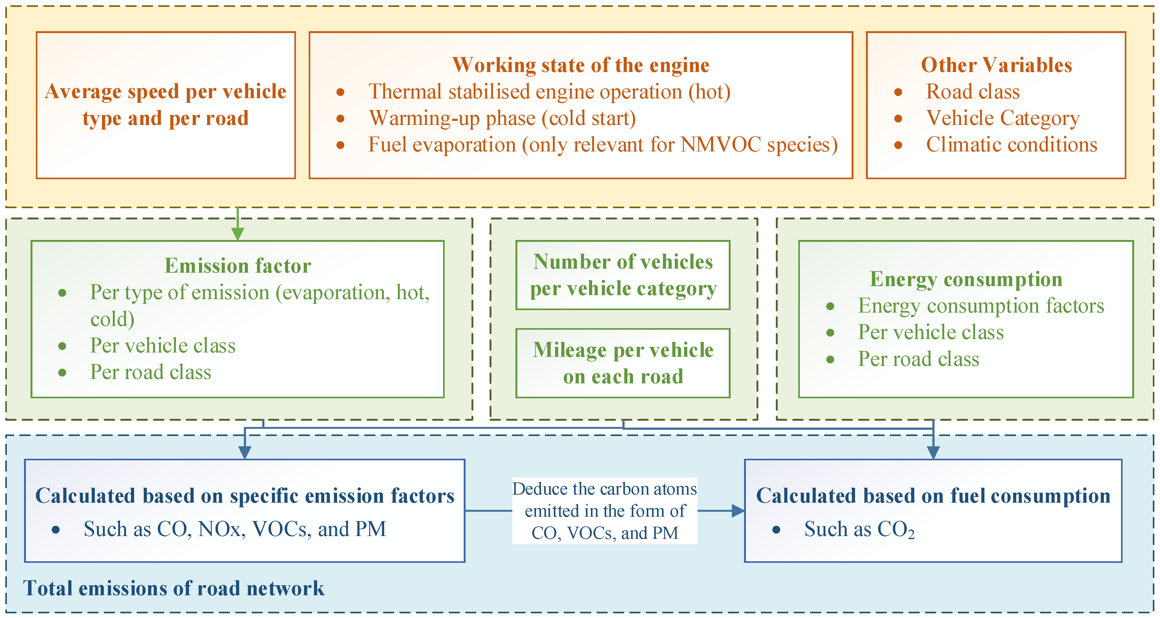
3.3. Travel Emission Calculation Model

The common emission models can be categorized into two main types: those based on driving conditions and those based on average speed. Emission models based on the vehicle-specific power (VSP) distribution, such as IVE and MOVES (Motor Vehicle Emission Simulator), focus on the actual driving conditions of vehicles. They are suitable for micro-scale studies and emphasize the impact of vehicle operating conditions on energy consumption emissions. However, these models typically require high-quality traffic data and often necessitate the integration of actual survey data.

On the other hand, emission models based on average speed include the MOBILE (Mobile Source Emission Factor Model) and COPERT (Computer Programme to Calculate Emissions from Road Transport) models. They are suitable for macro- and meso-scale studies and are commonly used for estimating traffic emissions and analyzing trends. Among them, the COPERT model, developed by the European Environment Agency (EEA), has the capability to calculate emissions for multiple pollutant species from various vehicle classifications. The emission standard in this model is compatible with the current vehicle emission control standards in China. Therefore, this study chose the COPERT model to analyze the emissions generated by ride-hailing. The model adopts a bottom-up approach for traffic emission calculations, as depicted in Figure 1.

Based on available data and calculation methods, COPERT categorizes pollutants into two groups. One group is calculated based on specific emission factors that are influenced by traffic conditions and engine parameters, such as CO, NO_x, VOCs, and PM. The other group, including CO₂ emissions, is computed based on fuel consumption. Depending on the operating conditions of the engine, COPERT divides the emission calculation of pollutant $k$ in the first group into three parts as follows:

$$E_{total}^k=E_{hot}^k+E_{cold}^k+E_{evap}^k$$

(12)

where $E_{total;i,j}^k\left[\mathrm{g}\right]$ represents the total emissions of pollutant $k$. $E_{hot}^k\left[\mathrm{g}\right]$ is the emissions during normal engine operation at operating temperature (hot stabilized emissions). $E_{cold}^k$ $\left[\mathrm{g}\right]$ is the emissions during transient engine warm-up processes (cold start emissions). $E_{evap}^k\left[\mathrm{g}\right]$ is the fuel evaporation emissions.

The calculation formula for the hot stabilized emissions $E_{hot}^k$ is as follows:

$$E_{hot}^k={\sum }_{i,j}{E}_{hot;i,j}^k$$

(13)

$$E_{hot;i,j}^k={VKT}_{i,j}\times N_{i,j}\times {EF}_{hot;i,j}^k$$

(14)

$${EF}_{hot;i,j}^k=\frac{{\alpha }_k\times {V_{i,j}}^2+{\beta }_k\times V_{i,j}+{\gamma }_k+{\delta }_k/V_{i,j}}{{\epsilon }_k\times {V_{i,j}}^2+{\zeta }_k\times V_{i,j}+{\eta }_k}$$

(15)

where $E_{hot;i,j}^k\left[\mathrm{g}\right]$ represents the hot stabilized emissions from vehicle type $j$ on road segment $i$. ${VKT}_i$ $[\mathrm{k}\mathrm{m}/\mathrm{v}\mathrm{e}\mathrm{h}.]$ and $N_{i,j}$ [$\mathrm{v}\mathrm{e}\mathrm{h}.]$ are the travel distance and number of vehicle type $j$ on road segment $i$. ${EF}_{hot:i,j}$ $[\mathrm{g}/\mathrm{k}\mathrm{m}]$ is the hot stabilized emissions factor. It can be calculated based on the average speed of vehicle type $j$ on road segment $i$, as shown in Equation (15). The coefficients in Equation (15) are detailed in the COPERT model and are associated with factors such as vehicle type, emission standards, and fuel type.

The calculation formula for the cold start emissions $E_{cold}^k$ is as follows:

$$E_{cold}^k={\sum }_j{E}_{cold;j}^k$$

(16)

$$E_{cold;j}^k={VKT}_j\times N_j\times {EF}_{hot;j}^k\times ({EF}_{cold;j}^k/{EF}_{hot;j}^k-1)\times {\beta }_j$$

(17)

$${EF}_{cold;j}^k/{EF}_{hot;j}^k=A_k\times V_j+B_k\times t_a+C_k$$

(18)

$${\beta }_j=0.6474-0.02545\times I_{trip,j}-(0.00974-0.000385\times I_{trip,j})\times t_a$$

(19)

where ${EF}_{cold;j}^k/{EF}_{hot;j}^k$ is the cold-over-hot ratio of vehicle type $j$. Similar to the heat emission factor, it can be calculated using an expression related to the vehicle’s average speed $V_j$ and the monthly average temperature $t_a$ [°C], as shown in Equation (18). The coefficients $A_k$, $B_k$, and, $C_k$ also have been obtained in the COPERT model. ${\beta }_j$ represents the proportion of the mileage of vehicle type $j$ during the cold start phase. It depends on the monthly average temperature $t_a$ and the driving pattern of vehicle, particularly the average travel distance $I_{trip,j}$ [$\mathrm{k}\mathrm{m}$].

The calculation formula for fuel evaporation emissions $E_{evap}^k$ is as follows:

$$E_{evap}^k=365\times N_{i,j}\times (e^d+S^c+S^{fi})+R$$

(20)

where $e^d$ $[\mathrm{g}/\mathrm{v}\mathrm{e}\mathrm{h}.]$ is emission factor for diurnal losses, which is correlated with environmental temperature, temperature difference, and fuel volatility. $S^c$ $[\mathrm{g}/\mathrm{v}\mathrm{e}\mathrm{h}.]$ and $S^{fi}$ $[\mathrm{g}/\mathrm{v}\mathrm{e}\mathrm{h}.]$ represent the average hot emission factor of gasoline powered vehicles equipped with carburetor and fuel injection. $R$ is the hot running losses.

The calculation of CO₂ emissions is based on fuel consumption. It is noteworthy that in this process, the deduction of carbon atoms emitted in the form of CO, VOCs, and PM needs to be considered. The calculation formula is as follows:

$$E_{total}^{{CO}_2}=44.011\times \frac{{FC}_{total}}{12.011+1.008r_{H:C}}-\frac{E_{total}^{CO}}{28.011}-\frac{E_{total}^{VOC}}{13.85}-\frac{E_{total}^{PM}}{12.011}$$

(21)

where $E_{total}^{{CO}_2}$ $\left[\mathrm{g}\right]$, $E_{total}^{CO}\left[\mathrm{g}\right]$, $E_{total}^{VOC}$ $\left[\mathrm{g}\right]$, and $E_{total}^{PM}$ $\left[\mathrm{g}\right]$ are the total emission of CO₂, CO, VOC, and PM, respectively. ${FC}_{total}$ $\left[\mathrm{T}\mathrm{J}\right]$ represents the fuel consumption. Its calculation method is similar to that of hot stabilized emissions, with the difference being the substitution of energy consumption factors for hot emission factors. $r_{H:C}$ is the ratio of hydrogen to carbon atoms in the fuel.

4. Data Description and Processing

4.1. Study Area

The experiment was conducted in Shenzhen City, Guangdong Province, China. Shenzhen City comprises nine administrative districts (Futian, Luohu, Nanshan, Yantian, Bao’an, Longgang, Longhua, Pingshan, and Guangming) and one functional area (Dapeng). Among them, the highlighted areas (Futian, Luohu, and Nanshan) are considered the urban centers. Transportation Analysis Zones (TAZs) are spatial units delineated based on a comprehensive consideration of factors such as transportation, land use, and population, providing a more comprehensive reflection of urban spatial characteristics and traffic conditions. Therefore, this study adopted TAZs as spatial analysis units and divided Shenzhen city into several TAZs based on previous research [80]. To obtain more accurate analysis results, the Dapeng area with fewer travel records and sparse traffic route distributions, as well as some TAZs with zero information, were excluded. Finally, 470 TAZs were obtained, as shown in Figure 2. Additionally, to observe the detailed spatio-temporal effects of variables on ride-hailing travel emissions, this study chose a time scale of 1 h as the time analysis unit, dividing one day into 24 time slots.

4.2. Dependent Variables

This study aims to analyze the spatio-temporal heterogeneity of key factors affecting emissions from ride-hailing services using the U-GTWR model. The average emission rate of ride-hailing services (emissions produced per kilometer on average) serves as the dependent variable in the model. It is calculated based on the vehicle trajectory data from both taxis and ride-hailing vehicles. The vehicle trajectory data are sourced from the Transport Operation Command Center (TOCC), recording vehicle movement information every 30 s. It includes vehicle license plate numbers, latitude–longitude positions, speed, travel angles, and corresponding timestamps.

This work extracted vehicle trajectory data from May 2019 (excluding the public holidays from 1 to 5 May) to compute the emissions of ride-hailing. During this process, it is necessary to differentiate between gasoline-powered vehicles and new energy vehicles in the vehicle trajectories. The most direct distinction between them lies in the license plate. The first difference is the color of the license plates. License plates for new energy vehicles are green, while those for gasoline-powered cars are blue. The second difference is the number of digits on the license plate. License plates for new energy vehicles consist of six digits, whereas those for gasoline-powered cars consist of five digits. Based on this, we can extract the trajectories of gasoline vehicles. Due to differences in travel patterns, destinations, and times between weekdays and weekends, the emissions from the two may differ. Therefore, the travel trajectories were further divided into weekdays and weekends for analysis. Subsequently, the trajectories were corrected and matched to the road network using map-matching algorithm technology. Then, based on the COPERT model, the total CO₂ emissions from ride-hailing trips were calculated for each hour. Finally, the emission rate of ride-hailing trips per hour in each TAZ was obtained by dividing the emission volume of each TAZ per hour by the total length of road segments in the TAZ.

Figure 3 illustrates the spatial distribution of the average CO₂ emission rate of ride-hailing travel during the morning and evening peak hours on weekdays and weekends. The spatial distribution of carbon emissions is characterized by non-uniformity. Specifically, downtown areas such as the Nanshan, Futian, and Luohu districts exhibit relatively higher average emission rates, which gradually decrease towards the city outskirts. Main arterial roads also display significant emission hotspots, with lower-grade roads connected to these arteries forming scattered local hotspots. Moreover, the average emission rates during morning peak hours surpass those during evening peak hours, and emissions are generally higher on weekdays compared to weekends.

4.3. Independent Variables

As for the independent variables of the U-GTWR model, we categorize them into four categories based on previous studies: travel demand, land use, demographic characteristics, and transportation network features. First, understanding the demand for different modes of transportation can help city planners in market positioning for ride-hailing services and in formulating more rational urban transportation policies, such as improving public transportation and planning road networks. This can impact the demand and emissions of ride-hailing trips, thereby promoting the development of sustainable modes of travel. This study separately considers the travel demand for four modes: bus, metro, shared bikes, and ride-hailing services. The travel dataset involved includes vehicle order data and smart card data. Specifically, the spatial and temporal distribution of bus and metro travel demand can be obtained from the smart card data, which records the boarding stations and times of passengers taking buses or metros. On the other hand, the spatial and temporal distribution of ride-hailing and bike-sharing travel demand can be obtained from the vehicle order data. The data records the latitude and longitude positions and times of vehicle pickups (or unlocking). Figure 4 illustrates the spatial distribution patterns of the daily demand for these four travel modes. It is evident that there are significant spatial variations in the travel demand for the four modes. Bus travel demand is evenly distributed throughout the study area, with a large number of trips occurring in the city center and fewer trips in peripheral areas. Metro travel demand is mainly concentrated in the western and southern parts of the city, where metro lines are densely distributed. The majority of bike-sharing and ride-hailing trips are concentrated in the central and southern parts of the city (specifically, the areas of Luohu, Futian, and Nanshan), while travel in other areas is relatively sparse.

The second category of factors considered is related to land use. Land use affects the spatial distribution of travel demand and the selection of travel modes, thus influencing regional travel emissions. Consequently, this study examines the impact of different types of land use on emissions from ride-hailing trips. The land-use variables are derived from point-of-interest (POI) data, represented by the average number of POI points per square meter. The POI data were obtained from Amap (https://ditu.amap.com/, accessed on 31 May 2019). However, the direct utilization of this data for discussion and research is not feasible due to inconsistencies between the classification standards of the POI data and urban land-use standards, as well as issues such as data redundancy and semantic duplication. Therefore, data preprocessing was conducted on the raw POI data. Firstly, missing and abnormal values were deleted to prevent any potential biases in the analysis. Then, duplicate data entries were removed to eliminate redundancy and streamline the dataset. Additionally, points with lower public awareness were excluded to enhance the interpretability and relevance of the research. Similar categories within the remaining POI data were merged based on land-use classification files and previous literature. Finally, land-use variables were grouped into six categories: commercial land, residential land, leisure land, catering land, public service land, and transportation facility land. Moreover, the presence of mixed-use areas also influences ride-hailing demand. Consequently, the extent of land-use mixing was measured by calculating the land-use entropy index.

Furthermore, population variables are key factors influencing emissions from ride-hailing services. This is because densely populated residential areas typically increase the demand for ride-hailing, especially in areas with limited public transportation access. Residents in these areas may prefer ride-hailing services as alternative commuting options. In this study, population data obtained from the WorldPop website (https://www.worldpop.org/, accessed on 31 May 2019) was used to calculate the population density per square meter within each TAZ region as a population variable. Additionally, the employment population within commercial areas may require more frequent business travel, where ride-hailing services could be a convenient transportation choice. Hence, the distribution of the employment population may also affect ride-hailing emissions. We further computed the employment population density within each TAZ region using employment data obtained from the Shenzhen Statistical Bureau.

Regarding the characteristics of the transportation network, in addition to the commonly considered indexes such as route density and station density, this study incorporates the accessibility and betweenness centrality of road network nodes. The accessibility of public transportation stations reflects the quality of service provided to passengers and is a critical factor influencing the choice of travel mode for surrounding travelers. If the availability of public transportation options is limited, people may rely more on ride-hailing services, thereby increasing the emissions generated by ride-hailing trips. In this study, we employ an accessibility analysis method based on minimum impedance [81] to calculate the accessibility of road network nodes. This method utilizes the average minimum impedance from a central point to all destination points as the accessibility evaluation indicator for the central point. The accessibility $A_i$ of node $i$ on the network can be calculated as follows:

$$A_i=\frac{1}{n-1}\sum _{\begin{array}{c}j=1\\ j\ne i\end{array}}^n(d_{ij})$$

(22)

where $d_{ij}$ [$\mathrm{m}\mathrm{i}\mathrm{n}$] represents the minimum time impedance between node $i$ and node $j$. The minute is chosen as the unit for accessibility because it can provide sufficient precision and is more aligned with people’s perceptions of time in daily life. It is more common and applicable in traffic planning and analysis, as shown in previous studies [82,83,84]. After obtaining the accessibility values for each node on the network, the inverse distance weighted (IDW) method is utilized to interpolate and estimate the accessibility of each TAZ unit. Based on the aforementioned approach, the accessibility of both the bus and metro network stations is computed, as depicted in Figure 5. The results reveal a gradual decrease in accessibility from the city center, particularly in the Futian District, towards the surrounding areas. This trend aligns with the denser concentration of public transportation stations in the city center, indicating a higher quality of public transportation services in this area compared to others.

Betweenness centrality measures the importance of nodes in a network by assessing their capacity to link diverse regions in the road network. Nodes characterized by higher betweenness centrality are usually pivotal intersections, as they frequently accommodate substantial traffic volume, thereby potentially exerting a considerable influence on travel emissions. The calculation of betweenness centrality for road network nodes follows the formula below:

$$C_B(i)=\sum _{s\ne i\ne t\in N}\frac{\sigma (s,t|i)}{\sigma (s,t)}$$

(23)

where $\sigma (s,t|i)$ represents the number of shortest paths between nodes $s$ and $t$ passing through node $i$, while $\sigma (s,t)$ denotes the total number of shortest paths between nodes $s$ and $t$. And the shortest path refers to minimizing the number of edges along the path. The betweenness centrality of TAZ is the average betweenness centrality value of the nodes located within that TAZ unit. The distribution of betweenness centrality for nodes in the bus network, metro network, and road network is illustrated in Figure 6. High-betweenness-centrality nodes in bus and metro networks are often crucial interchange stations, while high-betweenness-centrality nodes in road networks may serve as transportation hubs, such as intersections of major roads and minor roads. As shown in Figure 6, high-betweenness-centrality nodes in bus and road networks are evenly distributed. This is because the bus network and road network constitute the primary urban transportation infrastructure, necessitating comprehensive coverage in the entire city to cater to diverse travel demands. Such a designed transportation network can enhance accessibility and traffic flow throughout the city. In contrast, the metro system is concentrated in densely populated and high-demand areas within the city center, where high-betweenness-centrality nodes in the metro network are also clustered. This centralized metro network is designed to more effectively alleviate pressure on road traffic and mitigate environmental pollution.

4.4. Variable Statistics and Screening

Overall, we have compiled the values of each variable in different TAZ units for each hour of the day, resulting in a total sample size of $470\times 24=\mathrm{11,280}$. The statistical results are presented in

Table 1. Statistics and description of the variables.

Variable			Average	Standard Deviation	Description
Dependent variable
Ride-hailing emissions (Weekdays)		y	5.8110	12.2199	Emissions generated by ride-hailing travel per kilometer per hour on weekdays (kg/km)
Ride-hailing emissions (Weekend)			5.6494	12.4222	Emissions generated by ride-hailing travel per kilometer per hour on weekend (kg/km)
Independent variable
Travel demand (4)	Bus ridership (Weekdays)	x1	2.8636	2.4140	Natural logarithm of bus ridership per hour on weekdays
	Bus ridership (Weekend)		2.8300	2.3120	Natural logarithm of bus ridership per hour on weekend
	Metro ridership (Weekdays)	x2	1.0108	2.2659	Natural logarithm of metro ridership per hour on weekdays
	Metro ridership (Weekend)		0.9992	2.2293	Natural logarithm of metro ridership per hour on weekend
	Ride-hailing ridership (Weekdays)	x3	2.2241	2.1606	Natural logarithm of ride-hailing ridership per hour on weekdays
	Ride-hailing ridership (Weekend)		2.3599	2.0628	Natural logarithm of ride-hailing ridership per hour on weekend
	Bike-sharing ridership (Weekdays)	x4	1.9100	2.2343	Natural logarithm of bike-sharing ridership per hour on weekdays
	Bike-sharing ridership (Weekend)		3.7078	1.7060	Natural logarithm of bike-sharing ridership per hour on weekend
Land use (7)	Commercial land density	x5	155.4727	184.6213	The number of commercial lands per square kilometer
	Residential land density	x6	43.1141	50.6933	The number of residential lands per square kilometer
	Leisure land density	x7	53.1142	62.0186	The number of leisure lands per square kilometer
	Catering land density	x8	83.5013	96.3907	The number of catering lands per square kilometer
	Public service land density	x9	88.2451	101.3098	The number of public service lands per square kilometer
	Transportation facility land density	x10	47.7839	66.0291	The number of transportation facilities lands per square kilometer
	Land-use entropy index	x11	1.0718	0.2685	The index to evaluate the diversity of land use
Demographics (2)	Population density	x12	14.4973	14.4888	The number of people per square kilometer
	Employed population density	x13	1.8321	1.9911	The number of employed people per square kilometer
Traffic network structure (10)	Bus lines density	x14	91.7586	230.2714	The length of bus lines per square kilometer (km−1)
	Bus stations density	x15	45.1554	42.0940	The number of bus stations per square kilometer
	Bus accessibility	x16	27.7111	7.3157	The accessibility of bus stations (min)
	Bus network betweenness centrality	x17	0.0138	0.0182	The average values of betweenness centrality of nodes in the bus network
	Metro lines density	x18	1.8434	3.0026	The length of metro lines per square kilometer (km−1)
	Metro stations density	x19	0.3129	1.6045	The number of metro stations per square kilometer
	Metro accessibility	x20	39.6499	11.5565	The accessibility of metro stations (min)
	Metro network betweenness centrality	x21	0.0157	0.0384	The average values of node betweenness centrality in the metro network
	Road network density	x22	12.0990	7.6207	The length of road segments per square kilometer (km−1)
	Road network betweenness centrality	x23	0.0016	0.0023	The average values of node betweenness centrality in the road network

. To meet the normality assumption of the GTWR model, a logarithmic transformation is conducted on the travel counts [85].

Multicollinearity refers to the situation in a regression model where two or more independent variables exhibit a high degree of correlation. This condition can result in unstable estimates of regression coefficients, making it difficult to accurately estimate the effects of each independent variable on the dependent variable. In this study, the variance inflation factor (VIF) is introduced to evaluate the impact of multicollinearity. Based on multicollinearity tests, variables with VIF values greater than 7.5 were removed. Additionally, variables with insignificant correlation tests (p-value > 0.05) were also excluded. The remaining variables are listed in

Table 2. Results of the variable screening.

Variable		Weekdays (17)			Weekend (16)
		VIF	Coff.		VIF	Coff.
Bus ridership	x1	4.2756	0.0131		3.7600	−0.0143
Metro ridership	x2	1.8377	0.1401 ***	√	1.8401	0.1252 ***	√
Ride-hailing ridership	x3	7.3728	0.3482 ***	√	6.3744	0.3312 ***	√
Bike-sharing ridership	x4	5.2137	0.2664 ***	√		0.1702 ***
Commercial land density	x5	4.4186	0.2376 ***	√	4.4333	0.2041 ***	√
Residential land density	x6		0.3818 ***			0.3606 ***
Leisure land density	x7		0.3521 ***			0.3310 ***
Catering land density	x8	5.0998	0.2958 ***	√	5.1317	0.2805 ***	√
Public service land density	x9		0.3547 ***			0.3394 ***
Transportation facility land density	x10	6.6903	0.3993 ***	√	6.6972	0.3701 ***	√
Land-use entropy index	x11		−0.0634 ***			−0.0688 ***
Population density	x12	4.0244	0.3409 ***	√	4.0228	0.3243 ***	√
Employed population density	x13	3.3981	0.2784 ***	√	3.3857	0.2546 ***	√
Bus lines density	x14	1.3132	0.5893 ***	√	1.3135	0.6040 ***	√
Bus stations density	x15	5.4143	0.3075 ***	√	5.4157	0.2910 ***	√
Bus accessibility	x16	4.4289	−0.3185 ***	√	4.0165	−0.3053 ***	√
Bus network betweenness centrality	x17	1.7452	−0.0784 ***	√	1.7345	−0.0834 ***	√
Metro lines density	x18	1.8143	0.1614 ***	√	1.8158	0.1574 ***	√
Metro stations density	x19	1.6124	0.1467 ***	√	1.6140	0.1566 ***	√
Metro accessibility	x20		−0.4026 ***			−0.3863 ***
Metro network betweenness centrality	x21	1.3848	0.1242 ***	√	1.3778	0.1208 ***	√
Road network density	x22	6.6089	0.2769 ***	√	6.4430	0.2592 ***	√
Road network betweenness centrality	x23	1.4457	−0.0490 ***	√	1.4470	−0.0506 ***	√

(Note: *, **, and *** indicate significant at 90%, 95%, and 99% confidence levels, respectively).

. There are 17 variables affecting weekday ride-hailing emissions and 16 variables affecting weekend ride-hailing emissions, all of which have correlations with ride-hailing emissions at a 99% confidence level.

The difference in variable selection results between weekdays and weekends is the bike-sharing ridership variable. The correlation of bike-sharing ridership with ride-hailing emissions on weekdays is significant, whereas it appears insignificant on weekends. Therefore, the bike-sharing ridership variable is excluded from the analysis of ride-hailing emissions on weekends. This result is explainable. On weekdays, individuals typically face commuting needs, where bike-sharing may be more commonly used for short-distance commutes. Consequently, the usage of bike-sharing may compete with ride-hailing services on weekdays, resulting in a significant correlation. However, on weekends, individuals are inclined towards leisure and recreational activities. Bike-sharing is often utilized for short-distance leisure travel, while ride-hailing services may cater to specific needs such as returning home at night or traveling to particular destinations. This different usage demand may result in a weaker association between weekend bike-sharing trip volume and ride-hailing service emissions.

5. Results Analysis

5.1. Model Performance Comparison

The study compares proposed U-GTWR model with ordinary least square (OLS), GWR, and the GTWR model proposed by Huang et al. (hereinafter referred to as H-GTWR). Residual sum of squares ($RSS$), $R$-squared ($R^2$), and adjusted $R$-squared are utilized as performance metrics for model comparison. The computed performance metrics for each model are presented in Figure 7.

The OLS model does not account for the heterogeneity of variable distributions, assuming uniform regression coefficients for all observation points. It results in suboptimal $R^2$ and adjusted $R^2$. In contrast, the GWR model provides independent regression coefficients for each observation point, offering a more detailed analysis of potential spatially varying relationships between adjacent observation points. Compared to the OLS model, the GWR model exhibits a lower $RSS$ and a higher adjusted $R^2$, indicating better statistical performance. However, with an $R^2$ of only around 0.6, the GWR model’s consideration of heterogeneity is insufficient. The performance of both the GTWR and U-GTWR models indicates that extending the GWR model into the temporal dimension to address the spatio-temporal heterogeneity of variables significantly enhances the goodness of fit of the statistical outcomes. Particularly, regardless of analyzing weekday or weekend travel emissions, the U-GTWR model exhibits the best performance.

Compared to the H-GTWR model, the U-GTWR model exhibits a reduction in the RSS indicator by 60.2% and 63.5% for weekday and weekend analyses, respectively. Additionally, it increases the adjusted $R^2$ values by 9.8% and 10.8%, achieving explanatory powers of 94.4% and 94.7% for the spatio-temporal variations in ride-hailing travel emissions. These findings highlight the effectiveness of adaptively adjusting spatio-temporal bandwidths in capturing the spatio-temporal features of variables and enhancing model performance.

5.2. Spatio-Temporal Bandwidth Analysis

The U-GTWR model provides different spatio-temporal bandwidths $b_s$ and $b_t$ for all regression timestamps, as shown in

Table 3. Estimates of the spatio-temporal bandwidth.

Time	Weekdays		Weekend		Time	Weekdays		Weekend
	bs	bt (Unit: Hour)	bs	bt (Unit: Hour)		bs	bt (Unit: Hour)	bs	bt (Unit: Hour)
T1	0.2321	0	0.2319	0	T13	0.2181	1	0.2184	1
T2	0.2127	1	0.1296	1	T14	0.2307	6	0.2292	1
T3	0.1874	1	0.1980	2	T15	0.9966	1	0.9969	1
T4	0.1097	3	0.0422	3	T16	0.9996	1	0.9996	1
T5	0.0368	2	0.0296	3	T17	0.9993	1	0.9966	1
T6	0.0299	2	0.1291	1	T18	0.0341	17	0.0277	17
T7	0.1288	1	0.1300	1	T19	0.0287	2	0.0299	2
T8	0.1300	1	0.1303	1	T20	0.1966	1	0.2399	1
T9	0.1288	1	0.1322	1	T21	0.1417	1	0.1307	1
T10	0.1809	1	0.1300	1	T22	0.0311	2	0.0280	3
T11	0.1663	1	0.1641	1	T23	0.0299	3	0.0280	4
T12	0.2442	1	0.2342	1	T24	0.0322	2	0.0284	5

. For most timestamps, the temporal bandwidth $b_t$ of the U-GTWR model is approximately 1. This indicates that, in most instances, the data near the current timestamp significantly outweighs the influence of historical data on the model. Consequently, the model exhibits increased sensitivity and precision in considering spatio-temporal changes at these timestamps. However, for a few timestamps, such as $T_{18}$ (17:00–18:00), the temporal bandwidth $b_t$ extends to 17. This may be attributed to fluctuations in data within this time period or the occurrence of specific events, such as the evening peak hours. In such scenarios, the model adjusts the spatio-temporal bandwidth to better capture these sudden changes, ensuring the accuracy and robustness of the model.

The spatial bandwidth $b_s$ is expressed as the percentage of data points used in the estimation. A larger spatial bandwidth $b_s$ indicates that more neighboring observations are considered in the estimation process. In the analysis of weekday and weekend travel emissions utilizing the U-GTWR model, spatial bandwidth values exceeding 0.99 are observed during the regression timestamps between $T_{15}$ (14:00–15:00) and $T_{17}$(16:00–17:00). This could be attributed to the stronger spatial correlation of the data during the period from 14:00 to 17:00. This indicates that during these time intervals, the spatial distances between observation points have a more substantial influence on the model compared to temporal distances. Therefore, a larger spatial bandwidth is required to encompass a broader range of neighboring observations for a precise representation of spatio-temporal variations. Conversely, during other time intervals, due to the lower spatial correlation of the data, smaller spatial bandwidths are sufficient to meet the model’s requirements.

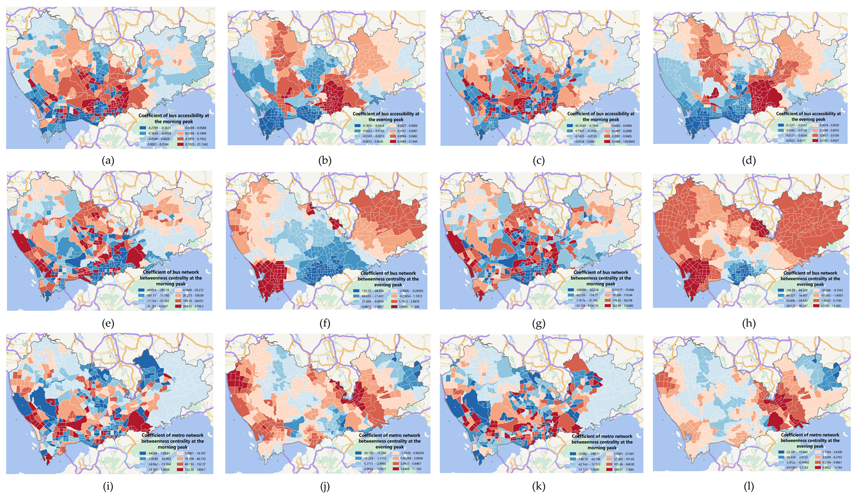
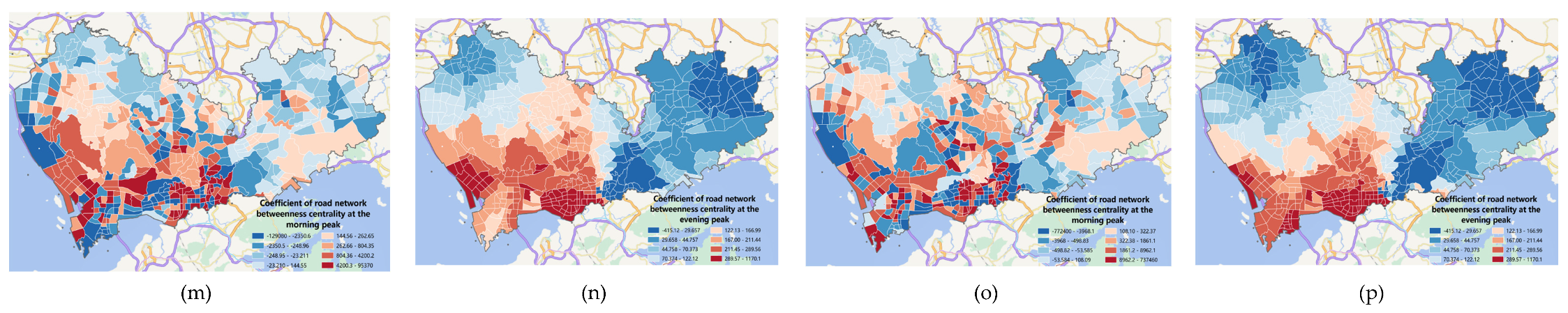
5.3. Analysis of Spatio-Temporally Heterogeneous Effects

As mentioned above, the U-GTWR model was utilized to explore the heterogeneous effects of various variables on ride-hailing travel emissions across different time and space regions.

Table 4. Coefficient estimates for spatio-temporally heterogeneous effects.

Variable		Mean	Std.	1st Qu.	Median	3st Qu.
Weekdays
Metro ridership	$x_2$	−0.326	2.298	−0.161	0.000	0.008
Ride-hailing ridership	$x_3$	0.778	1.513	0.037	0.326	1.342
Bike-sharing ridership	$x_4$	0.076	1.367	−0.080	0.028	0.370
Commercial land density	$x_5$	−0.005	0.544	−0.003	0.000	0.001
Catering land density	$x_8$	0.010	0.736	−0.003	0.000	0.013
Transportation facility land density	$x_{10}$	0.021	1.283	−0.002	0.004	0.033
Population density	$x_{12}$	0.015	3.935	−0.008	0.011	0.095
Employed population density	$x_{13}$	−0.275	53.937	−0.157	0.011	0.214
Bus lines density	$x_{14}$	0.097	7.853	0.001	0.007	0.030
Bus stations density	$x_{15}$	−0.059	6.996	−0.020	−0.002	0.003
Bus accessibility	$x_{16}$	−0.124	12.096	−0.002	0.004	0.040
Bus network betweenness centrality	$x_{17}$	600.883	62,502.976	−27.493	−1.228	2.058
Metro lines density	$x_{18}$	−1.896	265.719	−0.037	0.004	0.481
Metro stations density	$x_{19}$	5.843	791.567	−1.325	−0.040	0.313
Metro network betweenness centrality	$x_{21}$	−139.247	12,625.103	−5.726	−0.012	3.502
Road network density	$x_{22}$	−0.039	15.063	−0.187	−0.034	−0.002
Road network betweenness centrality	$x_{23}$	−795.522	222,774.734	12.203	96.892	320.894
Weekend
Metro ridership	$x_2$	−0.115	5.666	−0.089	0.000	0.008
Ride-hailing ridership	$x_3$	0.713	1.642	0.047	0.324	1.346
Commercial land density	$x_5$	−0.004	0.376	−0.004	0.000	0.001
Catering land density	$x_8$	0.002	0.573	−0.002	0.001	0.014
Transportation facility land density	$x_{10}$	0.042	1.576	−0.002	0.003	0.032
Population density	$x_{12}$	0.016	3.239	−0.012	0.006	0.090
Employed population density	$x_{13}$	−0.316	59.457	−0.094	0.010	0.194
Bus lines density	$x_{14}$	0.050	2.021	0.000	0.006	0.030
Bus stations density	$x_{15}$	−0.021	3.192	−0.022	−0.001	0.004
Bus accessibility	$x_{16}$	−0.074	10.763	−0.011	0.001	0.021
Bus network betweenness centrality	$x_{17}$	208.598	14,034.037	−23.521	−0.827	2.350
Metro lines density	$x_{18}$	−6.893	288.524	−0.025	0.002	0.436
Metro stations density	$x_{19}$	18.155	735.058	−0.983	−0.011	0.263
Metro network betweenness centrality	$x_{21}$	−44.587	2960.608	−3.061	0.233	5.470
Road network density	$x_{22}$	−0.034	20.334	−0.172	−0.023	0.001
Road network betweenness centrality	$x_{23}$	1044.160	148,441.500	8.592	91.820	332.229

presents the estimated coefficient values of the variables along with their corresponding statistical outcomes. The average value reflects the average impact of the variables on ride-hailing travel emissions, with a larger absolute coefficient value indicating a greater impact of the variable. Moreover, the standard deviation of the coefficients serves as a measure of the spatio-temporal heterogeneity. A higher standard deviation suggests a more pronounced spatio-temporal heterogeneity in the impact of the variable on travel emissions. In addition, the lower quartile, median, and upper quartile of the coefficients can reflect the relationship between the independent variables and ride-hailing travel emissions across different TAZs.

The betweenness centrality of traffic network nodes has the greatest influence on travel emissions, according to the average values of the coefficients. Furthermore, the standard deviation values indicate that the spatio-temporal heterogeneity of these variables is also significant, particularly within the road network. Quartile parameters and medians reveal a wider positive impact range of betweenness centrality in road network nodes. This is because the road network constitutes a core component of urban transportation networks. Nodes with higher betweenness centrality typically serve as critical hubs for traffic flow, significantly influencing vehicle movement and congestion [86,87]. Increasing the betweenness centrality of road network nodes may encourage more traffic flow, consequently leading to increased emissions from ride-hailing services. Conversely, the negative impact range of betweenness centrality in bus network nodes is broader. This is because areas with higher betweenness centrality in bus network nodes often offer more convenient, economical, and environmentally friendly public transportation options [88]. This scenario can reduce the demand for ride-hailing services, subsequently decreasing emissions generated by ride-hailing travel. Additionally, the negative impact range of betweenness centrality in metro network nodes is broader on weekdays, compared with the wider positive impact on weekends. This variation may be attributed to different travel demands on weekdays and weekends. Consequently, elevating the betweenness centrality of metro network nodes may enhance the attraction of metro for commuters during the weekdays, facilitating a potential shift towards more sustainable transportation choices.

The impact of metro and bike-sharing ridership variables on ride-hailing travel emissions expresses a change from positive to negative. This indicates that metro and bike-sharing services play both substitutive and complementary roles in ride-hailing travel. This finding aligns with previous research results [89,90]. However, analyzing this issue from the perspective of spatio-temporal heterogeneity remains novel. In the GTWR model-based analysis, coefficients representing the impact of variables exhibit both positive and negative effects, which is a common phenomenon. This is because the GTWR model allows for local estimation of parameters at each spatial location to better adapt to local characteristics. The disparity in the spatio-temporal distribution of variables results in different directional effects of the same variable on the dependent variable across different spatio-temporal locations. This also underscores the importance of considering spatio-temporal differences in variables when accurately capturing geographic phenomena.

To visually analyze the spatio-temporally heterogeneous effects of variables, Figure 8, Figure 9 and Figure 10 illustrate the spatial distribution of the impact coefficients of travel demand and road network structure variables on travel emissions during peak hours on weekdays and weekends, respectively. The results indicate significant spatial non-stationarity in the coefficients. The spatial patterns of the coefficients are similar between weekdays and weekends, while significant differences are observed between the morning and evening peak periods.

As shown in Figure 8a–d, during the morning peak period, the impact of metro ridership on ride-hailing travel emissions mainly follows the distribution of metro lines. In densely populated downtown areas where metro lines are concentrated, the impact of metro ridership on ride-hailing travel emissions is positive during the morning peak period and negative during the evening peak period. It is interpretable. During the morning peak hours on weekdays, people typically face strict commuting time constraints because they need to arrive at their workplaces or other destinations on time [91]. Although the metro serves as a primary mode of commuting, highly concentrated commuting demand may lead to issues such as congestion, resulting in increased waiting times for passengers [92,93]. Additionally, metro stations may be located some distance away from passengers’ final destinations, requiring them to use alternative travel modes (such as walking, buses, bicycles, or ride-hailing services) to complete the last leg of their journey [94,95]. These reasons might prompt some passengers to opt for ride-hailing services instead of waiting for the metro, resulting in increased ride-hailing emissions. In contrast, during the evening peak hours, people generally have more flexibility with their time and are not as constrained by strict work schedules as during the morning peak hours. Therefore, some individuals may prefer to use public transportation such as the metro rather than ride-hailing services to save costs and time. Based on these findings, urban planners can attract more commuters to choose the metro as their primary commuting mode during peak hours by improving the convenience, operational efficiency, and service quality of the metro. This approach could help alleviate ride-hailing emissions during peak hours.

Furthermore, we further observed that although the distributions on weekends and weekdays are similar, the positive impact of metro ridership on ride-hailing travel emissions is more widespread during the morning peak period on weekends. This suggests that in this period, the substitutive effect of metro travel on ride-hailing travel is weaker. This may be because the layout of metro lines primarily connects major activity areas of the city. Weekend travel demands may involve various destinations, some of which may not be fully accessible via metro lines, especially in peripheral areas of the city. In contrast, ride-hailing can more flexibly adapt to demand in different areas, resulting in a relatively weaker substitutive effect of metro travel on ride-hailing demand during this period. Similar findings have been reported in previous literature [13,96]. Therefore, in urban planning, it is essential to consider the layout of metro lines and the demand in surrounding areas, optimizing metro coverage to better meet travel demands during the weekend morning peak period.

The positive impact of ride-hailing ridership on ride-hailing travel emissions is predominantly concentrated in downtown areas, regardless of the time of day or week. The spatial distribution of coefficients is similar between weekends and weekdays, with slightly larger absolute values observed on weekdays, as shown in Figure 8e–h. This phenomenon is because downtown areas typically serve as commercial and office districts, which may generate more business trips and office commutes on weekdays, thereby increasing the demand for ride-hailing travel [97,98]. The Nanshan District demonstrates a more significant positive impact on ride-hailing travel emissions during evenings and weekends. This could be due to the concentration of commercial and entertainment establishments in this area [99], prompting individuals to opt for ride-hailing services during these periods. Hence, to mitigate congestion and emissions in downtown areas, various measures can be implemented. These include the implementation of time-based taxi service policies, the dynamic adjustment of taxi numbers based on demand fluctuations to improve operational efficiency, and the promotion of low-emission vehicles such as electric cars to reduce traffic emissions.

As described in Section 4.4, the bike-sharing ridership variable shows a significant correlation with ride-hailing travel emissions on weekdays but not on weekends. Figure 9 illustrates the spatio-temporal heterogeneity effect of bike-sharing ridership on ride-hailing travel emissions during peak hours on weekdays. In the Luohu District, bike-sharing travel demand shows negative and positive impacts during the morning and evening peaks, respectively. This disparity arises from the preference for shared bicycles over ride-hailing services during the morning rush hour, particularly for short-distance commuting, to circumvent road congestion constraints, save time, and reduce costs [96,100]. Consequently, shared bicycles contribute to a reduction in ride-hailing travel emissions. Conversely, residents may opt for ride-hailing services when returning home during the evening peak, particularly in low-light or adverse weather conditions. In such scenarios, the utilization rate of bike-sharing services may be relatively low, and the substitution effect of bike-sharing travel on ride-hailing travel is not significant, potentially even leading to an increase in demand for ride-hailing services.

Compared to Luohu District, Nanshan District and the western areas of Futian District have opposite effects during morning and evening peaks. Additionally, in the eastern regions of Futian District, bike-sharing demand shows a positive impact during both morning and evening peaks. This could be due to variances in urban land-use planning and transportation networks across different regions, leading to disparities in the suitability of bike-sharing and ride-hailing services during different time periods [89,101]. Specifically, bike-sharing may be better suited for short trips in the Luohu District, while commuting demands in Futian and Nanshan Districts might lean towards ride-hailing services. Therefore, policymakers can develop region-specific policies considering the disparities in the applicability of bike-sharing and ride-hailing services across different time periods. These policies have the potential to foster the advancement of environmentally friendly transportation options that better align with the needs of residents. For regions such as Luohu District, where bike-sharing demand shows a negative impact during morning peaks, government initiatives can promote bike-sharing for short-distance commutes. This can be achieved through the provision of cycling infrastructure, the establishment of bike lanes, and other measures aimed at reducing reliance on ride-hailing services. Additionally, to enhance the competitiveness of bike-sharing during evening peaks, collaborative efforts between the government and relevant enterprises can focus on enhancing the quality of bike-sharing services. This may involve improving bike maintenance standards, increasing the availability of parking spots, and enhancing the overall user experience. These actions aim to encourage residents to opt for bike-sharing as a preferred mode of transportation during various timeframes.

Figure 10 illustrates the spatio-temporal distribution of estimated coefficients related to the traffic network structure variables. The positive impact of bus accessibility on ride-hailing travel emissions is primarily concentrated in the central region of Shenzhen city, while the negative impact is particularly evident in the Nanshan and Futian districts during the evening peak period, as shown in Figure 10a–d. This is because Nanshan and Futian Districts serve as central business districts with a concentration of commercial, office, and service facilities, as well as a highly accessible public transportation network [99,102]. Travelers in the regions may prefer using public transit services for convenience or to reach destinations in the city center without relying on ride-hailing services, leading to a suppressive effect of bus accessibility on ride-hailing travel emissions. This effect is particularly pronounced during the evening peak period. In the central region, there are also important transportation hubs or intersections, as shown in Figure 6. Bus stops located in these areas often become popular spots for ride-hailing services [103]. Despite the enhanced accessibility of buses in these regions, individuals may still prefer opting for ride-hailing services due to their travel preferences [104]. Consequently, in these localities, bus accessibility tends to positively impact ride-hailing travel emissions. To mitigate this phenomenon, urban managers can further enhance the quality of public transportation services in the central areas by increasing bus routes, improving service frequency, and introducing intelligent bus systems. By improving the convenience and appeal of public transit options, they can decrease residents’ dependence on ride-hailing services. Moreover, setting up appropriate traffic signs and guidance systems at transportation hubs or intersections, along with providing convenient transfer facilities, are also effective measures to encourage residents to choose public transportation over ride-hailing services in these areas.

As shown in Figure 10i–p, the influence of network node betweenness centrality on ride-hailing travel emissions during the morning peak period appears to be more scattered across different travel modes, whereas it becomes more concentrated during the evening peak period. This phenomenon may be due to the widespread distribution of commuting activities and the complex traffic conditions during the morning peak period. The morning peak period typically represents the most congested period in urban transportation, characterized by heavy traffic flow and easily obstructed road sections [105]. Nodes with high betweenness centrality are prone to becoming bottlenecks in traffic congestion [87,106]. Surrounding these high-betweenness nodes, traffic flow may increase, leading to more emissions from ride-hailing traffic. Consequently, the positive and negative impacts of betweenness centrality on ride-hailing travel emissions are more scattered during the morning peak period, resembling the distribution observed in Figure 6. In contrast, during the evening peak period, there are significant differences in the influence of network node betweenness centrality on ride-hailing travel emissions among different travel modes. For instance, bus network node betweenness centrality exhibits a negative impact in the Futian district, while metro and road network node betweenness centrality show positive impacts. This implies that enhancing the betweenness centrality of bus network nodes in this area can help suppress the demand for ride-hailing travel. Specific policy measures may include increasing the density of bus routes in the Futian district, particularly those connecting important nodes within the district, and optimizing the planning of bus routes to ensure coverage of key commercial, residential, and office areas. In summary, the spatio-temporally heterogeneous effects of different network node betweenness centralities reflect variations in the competitiveness of different travel modes and residents’ travel preferences across different time periods. Therefore, urban managers should thoroughly understand the characteristics of each area when formulating urban transportation planning and management policies, and adopt differentiated strategies to promote more sustainable and low-carbon travel modes.

6. Conclusions

This study proposes a spatio-temporal geographically weighted regression model with an adaptive kernel function, aiming to explore the spatio-temporally heterogeneous effects of urban morphology and transportation-related factors on ride-hailing travel emissions. It comprehensively considers four categories of explanatory variables, comprising travel demand, land use, demographic statistics, and transportation networks. The traffic network structure plays a crucial role in influencing travel emissions by affecting traffic congestion levels and vehicle speeds. However, the impact mechanism for traffic network structures on travel emissions remains insufficiently explained in the current literature. Therefore, this research specifically focuses on traffic network structural characteristics, such as betweenness centrality and accessibility in multi-modal networks, with the goal of providing a more comprehensive understanding of the relationship between multiple travel modes, urban spatial structure, and emissions. According to the results of the experiments conducted in Shenzhen city, the U-GTWR model developed in this study outperforms OLS, GWR, and GTWR, demonstrating superior adaptation to the spatio-temporal heterogeneity of data. This indicates that the adaptive kernel function, which dynamically adjusts the spatio-temporal bandwidth based on the data distribution, can effectively enhance the interpretability of the GTWR model. The research findings reveal that the U-GTWR model achieves approximately 95% explanatory power for the spatio-temporal variation of ride-hailing travel emissions. Through the analysis of the influence coefficient of the model, the spatio-temporally heterogeneous effects of relevant factors on ride-hailing travel emissions are further discussed, providing valuable insights into urban transportation planning and low-carbon initiatives.

The experiments indicate that the betweenness centrality of transportation networks has a significantly higher impact on ride-hailing travel emissions compared to other factors. This further confirms the crucial role of traffic network structures in promoting low-carbon transportation development. Based on these research findings, we can offer the following recommendations for optimizing transportation resource allocation, enhancing public transit service levels, and fostering sustainable urban transportation development:

(1)

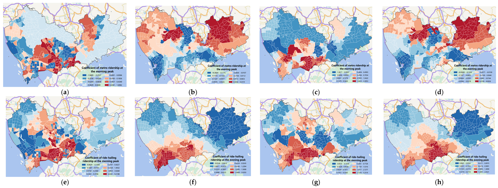
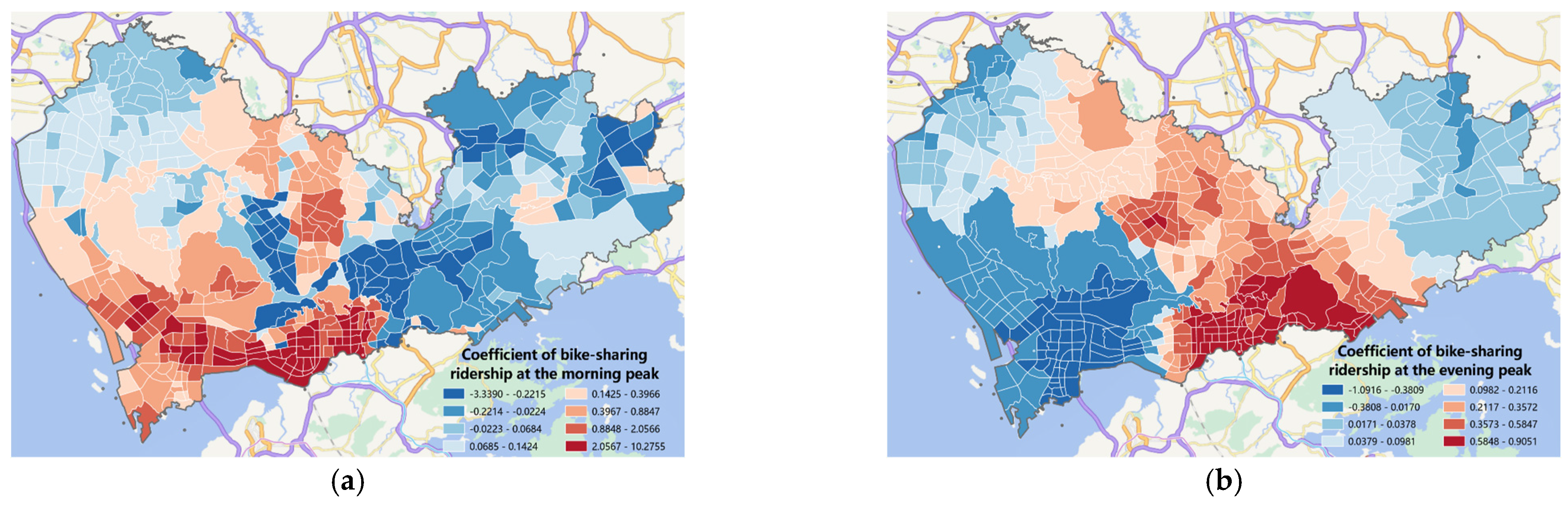
In terms of travel demand, the study found that metro travel demand in downtown areas has a positive impact on ride-hailing travel emissions during the morning peak and a negative impact during the evening peak. Therefore, urban managers can encourage more commuters to choose metro travel by improving the quality and efficiency of metro services. Additionally, it is important to consider the layout of metro lines and the surrounding areas’ demand to optimize the coverage of metro lines, better meeting the travel demand during weekend morning peaks. Moreover, considering the differences in the impact of bike-sharing and ride-hailing travel demand across different regions, region-specific policies should be adopted. For areas where bike-sharing demand has a negative impact, promoting the use of bike-sharing for short-distance commuting can reduce reliance on ride-hailing services. Conversely, for areas where bike-sharing demand has a positive impact, enhancing the quality of bike-sharing services can increase their competitiveness.

(2)

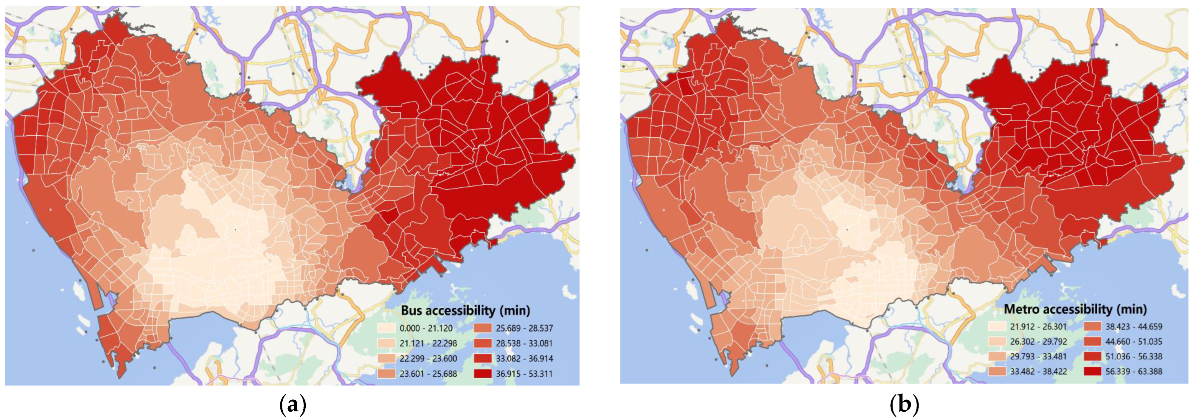
In terms of public transportation services, the study revealed that the impact of bus accessibility on ride-hailing travel emissions is primarily concentrated in the central areas of Shenzhen, with particularly significant negative effects observed in the Nanshan and Futian districts during the evening peak period. To address this phenomenon, urban managers can enhance the quality of bus services in central areas by increasing routes, improving frequency, and introducing intelligent systems to reduce the reliance of citizens on ride-hailing services. Additionally, measures such as installing traffic signs and providing transfer facilities at key areas such as transportation hubs and intersections can also encourage residents to choose public transportation. Furthermore, the impact of network node betweenness centrality on ride-hailing travel emissions appears to be more scattered during the morning peak period but more concentrated during the evening peak period. Therefore, urban managers should develop differentiated transportation planning and management policies based on the characteristics of each region to promote sustainable and low-carbon travel modes. For example, to address the negative impact of bus network node betweenness centrality in the Futian district, policy recommendations may include increasing bus route density and optimizing planning to cover important commercial, residential, and office areas.

These findings hold significant importance for mitigating urban traffic emissions and promoting the development of sustainable travel modes. While the applicability of the research findings to other regions may vary due to differences in urban infrastructure, transportation systems, and socio-economic factors, this methodological framework retains universal significance and can be applied across various cities. By integrating local urban morphology and transportation-related factors into the analysis, valuable insights can be provided for crafting carbon emission reduction strategies in different cities. It is important to note that the above policy recommendations directly stem from the analysis of regression coefficients obtained from the U-GTWR model. Therefore, through simulation or optimization techniques, further testing and validation of these recommendations would be valuable for future research. Additionally, it is essential to acknowledge the existing limitations in addressing the intricate nonlinear relationships among spatio-temporal characteristics. Future research endeavors would benefit from integrating additional machine learning or deep learning methodologies to enhance the model’s capacity for capturing complex relationships. Moreover, the U-GTWR model proposed in this study also presents numerous prospective applications in subsequent research. For instance, it can be utilized to devise transportation planning strategies and optimize urban spatial structures, addressing diverse facets such as travel demands, environmental conservation, and urban economic efficiency. Furthermore, the model also holds potential for integration into smart city platforms and mobile applications, facilitating the delivery of personalized travel advisory services tailored to urban residents.

References

1. Pant, P.; Harrison, R.M. Estimation of the contribution of road traffic emissions to particulate matter concentrations from field measurements: A review. Atmos. Environ. 2013, 77, 78–97. [Google Scholar] [CrossRef]
2. Birol, F. CO2 Emissions from Fuel Combustion Highlights, 2020th ed.; OECD/IEA: Paris, France, 2020. [Google Scholar]
3. Sui, Y.; Zhang, H.; Song, X.; Shao, F.; Yu, X.; Shibasaki, R.; Sun, R.; Yuan, M.; Wang, C.; Li, S.; et al. GPS data in urban online ride-hailing: A comparative analysis on fuel consumption and emissions. J. Clean. Prod. 2019, 227, 495–505. [Google Scholar] [CrossRef]
4. Zhao, P.; Kwan, M.-P.; Qin, K. Uncovering the spatiotemporal patterns of CO2 emissions by taxis based on Individuals’ daily travel. J. Transp. Geogr. 2017, 62, 122–135. [Google Scholar] [CrossRef]
5. Rodier, C. The Effects of Ride Hailing Services on Travel and Associated Greenhouse Gas Emissions. 2018. Available online: https://escholarship.org/uc/item/2rv570tt (accessed on 20 March 2024).
6. Rodier, C.; Michaels, J. The Effects of Ride-Hailing Services on Greenhouse Gas Emissions. 2019. Available online: https://escholarship.org/uc/item/4vz52416#main (accessed on 20 March 2024).
7. Tikoudis, I.; Martinez, L.; Farrow, K.; Bouyssou, C.G.; Petrik, O.; Oueslati, W. Ridesharing services and urban transport CO2 emissions: Simulation-based evidence from 247 cities. Transp. Res. Part D Transp. Environ. 2021, 97, 102923. [Google Scholar] [CrossRef]
8. Tirachini, A. Ride-hailing, travel behaviour and sustainable mobility: An international review. Transportation 2020, 47, 2011–2047. [Google Scholar] [CrossRef]
9. Wei, K.; Vaze, V.; Jacquillat, A. Transit planning optimization under ride-hailing competition and traffic congestion. Transp. Sci. 2022, 56, 725–749. [Google Scholar] [CrossRef]
10. Babar, Y.; Burtch, G. Examining the heterogeneous impact of ride-hailing services on public transit use. Inf. Syst. Res. 2020, 31, 820–834. [Google Scholar] [CrossRef]
11. Lv, Y.; He, L.; Sun, H.; Xu, G. Substituted Relationship between Ride-hailing and Public Transit and Emission Reduction Potential. J. Transp. Syst. Eng. Inf. Technol. 2023, 23, 11. [Google Scholar]
12. Luo, H.; Chahine, R.; Gkritza, K.; Cai, H. What motivates the use of shared mobility systems and their integration with public transit? Evidence from a choice experiment study. Transp. Res. Part C Emerg. Technol. 2023, 155, 104286. [Google Scholar] [CrossRef]
13. Li, X.; Du, M.; Zhang, Y.; Yang, J. Identifying the factors influencing the choice of different ride-hailing services in Shenzhen, China. Travel Behav. Soc. 2022, 29, 53–64. [Google Scholar] [CrossRef]
14. Loa, P.; Habib, K.N. Examining the influence of attitudinal factors on the use of ride-hailing services in Toronto. Transp. Res. Part A Policy Pract. 2021, 146, 13–28. [Google Scholar] [CrossRef]
15. Chen, J.; Li, W.; Zhang, H.; Cai, Z.; Sui, Y.; Long, Y.; Song, X.; Shibasaki, R. GPS data in urban online ride-hailing: A simulation method to evaluate impact of user scale on emission performance of system. J. Clean. Prod. 2021, 287, 125567. [Google Scholar] [CrossRef]
16. Ao, Y.; Yang, D.; Chen, C.; Wang, Y. Effects of rural built environment on travel-related CO2 emissions considering travel attitudes. Transp. Res. Part D Transp. Environ. 2019, 73, 187–204. [Google Scholar] [CrossRef]
17. Wu, X.; Tao, T.; Cao, J.; Fan, Y.; Ramaswami, A. Examining threshold effects of built environment elements on travel-related carbon-dioxide emissions. Transp. Res. Part D Transp. Environ. 2019, 75, 1–12. [Google Scholar] [CrossRef]
18. Shao, Q.; Zhang, W.; Cao, X.; Yang, J. Built environment interventions for emission mitigation: A machine learning analysis of travel-related CO2 in a developing city. J. Transp. Geogr. 2023, 110, 103632. [Google Scholar] [CrossRef]
19. Saberi, M.; Mahmassani, H.S.; Brockmann, D.; Hosseini, A. A complex network perspective for characterizing urban travel demand patterns: Graph theoretical analysis of large-scale origin–destination demand networks. Transportation 2017, 44, 1383–1402. [Google Scholar] [CrossRef]
20. Saberi, M.; Rashidi, T.H.; Ghasri, M.; Ewe, K. A complex network methodology for travel demand model evaluation and validation. Netw. Spat. Econ. 2018, 18, 1051–1073. [Google Scholar] [CrossRef]
21. Jenelius, E. Network structure and travel patterns: Explaining the geographical disparities of road network vulnerability. J. Transp. Geogr. 2009, 17, 234–244. [Google Scholar] [CrossRef]
22. Badia, H.; Argote-Cabanero, J.; Daganzo, C.F. How network structure can boost and shape the demand for bus transit. Transp. Res. Part A Policy Pract. 2017, 103, 83–94. [Google Scholar] [CrossRef]
23. Zheng, J.; Xu, M.; Li, R.; Yu, L. Research on group choice behavior in green travel based on planned behavior theory and complex network. Sustainability 2019, 11, 3765. [Google Scholar] [CrossRef]
24. Yang, Y.; Wang, C.; Liu, W. Urban daily travel carbon emissions accounting and mitigation potential analysis using surveyed individual data. J. Clean. Prod. 2018, 192, 821–834. [Google Scholar] [CrossRef]
25. Xu, B.; Lin, B. Factors affecting carbon dioxide (CO2) emissions in China’s transport sector: A dynamic nonparametric additive regression model. J. Clean. Prod. 2015, 101, 311–322. [Google Scholar] [CrossRef]
26. Gan, M.; Liu, X.; Chen, S.; Yan, Y.; Li, D. The identification of truck-related greenhouse gas emissions and critical impact factors in an urban logistics network. J. Clean. Prod. 2018, 178, 561–571. [Google Scholar] [CrossRef]
27. Xue, Y. Empirical research on household carbon emissions characteristics and key impact factors in mining areas. J. Clean. Prod. 2020, 256, 120470. [Google Scholar] [CrossRef]
28. Choi, K.; Zhang, M. The impact of metropolitan, county, and local land use on driving emissions in US metropolitan areas: Mediator effects of vehicle travel characteristics. J. Transp. Geogr. 2017, 64, 195–202. [Google Scholar] [CrossRef]
29. Ma, J.; Liu, Z.; Chai, Y. The impact of urban form on CO2 emission from work and non-work trips: The case of Beijing, China. Habitat Int. 2015, 47, 1–10. [Google Scholar] [CrossRef]
30. Qin, H.; Huang, Q.; Zhang, Z.; Lu, Y.; Li, M.; Xu, L.; Chen, Z. Carbon dioxide emission driving factors analysis and policy implications of Chinese cities: Combining geographically weighted regression with two-step cluster. Sci. Total Environ. 2019, 684, 413–424. [Google Scholar] [CrossRef] [PubMed]
31. Yuan, W.; Sun, H.; Chen, Y.; Xia, X. Spatio-Temporal evolution and spatial heterogeneity of influencing factors of SO2 Emissions in Chinese cities: Fresh evidence from MGWR. Sustainability 2021, 13, 12059. [Google Scholar] [CrossRef]
32. Cheng, R.; Zeng, W.; Zheng, Y. Exploring the Influence of Built Environment on Demand of Online Car-Hailing Travel Using Multi-Scale Geographically Temporal Weighted Regression Model. 2023. Available online: https://www.researchsquare.com/article/rs-3014459/v1 (accessed on 20 March 2024).
33. Kuonen, S. Estimating greenhouse gas emissions from travel–a GIS-based study. Geogr. Helv. 2015, 70, 185–192. [Google Scholar] [CrossRef]
34. Cao, X.; Yang, W. Examining the effects of the built environment and residential self-selection on commuting trips and the related CO2 emissions: An empirical study in Guangzhou, China. Transp. Res. Part D Transp. Environ. 2017, 52, 480–494. [Google Scholar] [CrossRef]
35. Christensen, L. Environmental impact of long distance travel. Transp. Res. Procedia 2016, 14, 850–859. [Google Scholar] [CrossRef]
36. Czepkiewicz, M.; Heinonen, J.; Ottelin, J. Why do urbanites travel more than do others? A review of associations between urban form and long-distance leisure travel. Environ. Res. Lett. 2018, 13, 073001. [Google Scholar] [CrossRef]
37. Akopov, A.S.; Beklaryan, L.A. Traffic Improvement in Manhattan Road Networks With the Use of Parallel Hybrid Biobjective Genetic Algorithm. IEEE Access 2024, 12, 19532–19552. [Google Scholar] [CrossRef]
38. Santos, O.; Ribeiro, F.; Metrôlho, J.; Dionísio, R. Using Smart Traffic Lights to Reduce CO2 Emissions and Improve Traffic Flow at Intersections: Simulation of an Intersection in a Small Portuguese City. Appl. Syst. Innov. 2023, 7, 3. [Google Scholar] [CrossRef]
39. Li, P.; Zhao, P.; Brand, C. Future energy use and CO2 emissions of urban passenger transport in China: A travel behavior and urban form based approach. Appl. Energy 2018, 211, 820–842. [Google Scholar] [CrossRef]
40. Xia, C.; Xiang, M.; Fang, K.; Li, Y.; Ye, Y.; Shi, Z.; Liu, J. Spatial-temporal distribution of carbon emissions by daily travel and its response to urban form: A case study of Hangzhou, China. J. Clean. Prod. 2020, 257, 120797. [Google Scholar] [CrossRef]
41. Hong, J.; Goodchild, A. Land use policies and transport emissions: Modeling the impact of trip speed, vehicle characteristics and residential location. Transp. Res. Part D Transp. Environ. 2014, 26, 47–51. [Google Scholar] [CrossRef]
42. Ding, C.; Wang, Y.; Xie, B.; Liu, C. Understanding the role of built environment in reducing vehicle miles traveled accounting for spatial heterogeneity. Sustainability 2014, 6, 589–601. [Google Scholar] [CrossRef]
43. Song, S.; Diao, M.; Feng, C.C. Individual transport emissions and the built environment: A structural equation modelling approach. Transp. Res. Part A Policy Pract. 2016, 92, 206–219. [Google Scholar] [CrossRef]
44. Yang, W.; Wang, S.; Zhao, X. Measuring the direct and indirect effects of neighborhood-built environments on travel-related CO2 emissions: A structural equation modeling approach. Sustainability 2018, 10, 1372. [Google Scholar] [CrossRef]
45. Barla, P.; Miranda-Moreno, L.F.; Lee-Gosselin, M. Urban travel CO2 emissions and land use: A case study for Quebec City. Transp. Res. Part D Transp. Environ. 2011, 16, 423–428. [Google Scholar] [CrossRef]
46. Zhu, X.; Li, R. An analysis of decoupling and influencing factors of carbon emissions from the transportation sector in the Beijing-Tianjin-Hebei Area, China. Sustainability 2017, 9, 722. [Google Scholar] [CrossRef]
47. Chow Alice, S.Y. Spatial-modal scenarios of greenhouse gas emissions from commuting in Hong Kong. J. Transp. Geogr. 2016, 54, 205–213. [Google Scholar] [CrossRef]
48. Ma, J.; Zhou, S.; Mitchell, G.; Zhang, J. CO2 emission from passenger travel in Guangzhou, China: A small area simulation. Appl. Geogr. 2018, 98, 121–132. [Google Scholar] [CrossRef]
49. Reichert, A.; Holz-Rau, C.; Scheiner, J. GHG emissions in daily travel and long-distance travel in Germany–Social and spatial correlates. Transp. Res. Part D Transp. Environ. 2016, 49, 25–43. [Google Scholar] [CrossRef]
50. Modarres, A. Commuting and energy consumption: Toward an equitable transportation policy. J. Transp. Geogr. 2013, 33, 240–249. [Google Scholar] [CrossRef]
51. Shim, G.E.; Rhee, S.M.; Ahn, K.H.; Chung, S.B. The relationship between the characteristics of transportation energy consumption and urban form. Ann. Reg. Sci. 2006, 40, 351–367. [Google Scholar] [CrossRef]
52. Qin, B.; Han, S.S. Planning parameters and household carbon emission: Evidence from high-and low-carbon neighborhoods in Beijing. Habitat Int. 2013, 37, 52–60. [Google Scholar] [CrossRef]
53. Zahabi, S.A.H.; Miranda-Moreno, L.; Patterson, Z.; Barla, P.; Harding, C. Transportation greenhouse gas emissions and its relationship with urban form, transit accessibility and emerging green technologies: A Montreal case study. Procedia-Soc. Behav. Sci. 2012, 54, 966–978. [Google Scholar] [CrossRef]
54. Sohrab, S.; Csikós, N.; Szilassi, P. Connection between the spatial characteristics of the road and railway networks and the air pollution (PM10) in urban–rural fringe zones. Sustainability 2022, 14, 10103. [Google Scholar] [CrossRef]
55. Zhou, S.; Lin, R. Spatial-temporal heterogeneity of air pollution: The relationship between built environment and on-road PM2.5 at micro scale. Transp. Res. Part D Transp. Environ. 2019, 76, 305–322. [Google Scholar] [CrossRef]
56. Yu, C.; Deng, Y.; Qin, Z.; Yang, C.; Yuan, Q. Traffic volume and road network structure: Revealing transportation-related factors on PM2.5 concentrations. Transp. Res. Part D Transp. Environ. 2023, 124, 103935. [Google Scholar] [CrossRef]
57. Çetin, M.; Sevik, H. Change of air quality in Kastamonu city in terms of particulate matter and CO2 amount. Oxid. Commun. 2016, 39, 3394–3401. [Google Scholar]
58. Glaeser, E.L.; Kahn, M.E. The greenness of cities: Carbon dioxide emissions and urban development. J. Urban Econ. 2010, 67, 404–418. [Google Scholar] [CrossRef]
59. Song, Y.; Miller, H.J.; Stempihar, J.; Zhou, X. Green accessibility: Estimating the environmental costs of network-time prisms for sustainable transportation planning. J. Transp. Geogr. 2017, 64, 109–119. [Google Scholar] [CrossRef]
60. De Coensel, B.; Can, A.; Degraeuwe, B.; De Vlieger, I.; Botteldooren, D. Effects of traffic signal coordination on noise and air pollutant emissions. Environ. Model. Softw. 2012, 35, 74–83. [Google Scholar] [CrossRef]
61. Brand, C.; Preston, J.M. ‘60–20 emission’—The unequal distribution of greenhouse gas emissions from personal, non-business travel in the UK. Transp. Policy 2010, 17, 9–19. [Google Scholar] [CrossRef]
62. Brand, C.; Goodman, A.; Rutter, H.; Song, Y.; Ogilvie, D. Associations of individual, household and environmental characteristics with carbon dioxide emissions from motorised passenger travel. Appl. Energy 2013, 104, 158–169. [Google Scholar] [CrossRef] [PubMed]
63. Lu, X.; Ota, K.; Dong, M.; Yu, C.; Jin, H. Predicting transportation carbon emission with urban big data. IEEE Trans. Sustain. Comput. 2017, 2, 333–344. [Google Scholar] [CrossRef]
64. Jermsittiparsert, K.; Chankoson, T. Behavior of tourism industry under the situation of environmental threats and carbon emission: Time series analysis from Thailand. Int. J. Energy Econ. Policy 2019, 9, 366–372. [Google Scholar] [CrossRef]
65. Shu, Y.; Lam Nina, S.N. Spatial disaggregation of carbon dioxide emissions from road traffic based on multiple linear regression model. Atmos. Environ. 2011, 45, 634–640. [Google Scholar] [CrossRef]
66. Yang, W.; Li, T.; Cao, X. Examining the impacts of socio-economic factors, urban form and transportation development on CO2 emissions from transportation in China: A panel data analysis of China’s provinces. Habitat Int. 2015, 49, 212–220. [Google Scholar] [CrossRef]
67. Xu, C.; Zhao, J.; Liu, P. A geographically weighted regression approach to investigate the effects of traffic conditions and road characteristics on air pollutant emissions. J. Clean. Prod. 2019, 239, 118084. [Google Scholar] [CrossRef]
68. Wu, J.; Jia, P.; Feng, T.; Li, H.; Kuang, H.; Zhang, J. Uncovering the spatiotemporal impacts of built environment on traffic carbon emissions using multi-source big data. Land Use Policy 2023, 129, 106621. [Google Scholar] [CrossRef]
69. Liu, J.; Li, S.; Ji, Q. Regional differences and driving factors analysis of carbon emission intensity from transport sector in China. Energy 2021, 224, 120178. [Google Scholar] [CrossRef]
70. Wang, S.; Shi, C.; Fang, C.; Feng, K. Examining the spatial variations of determinants of energy-related CO2 emissions in China at the city level using Geographically Weighted Regression Model. Appl. Energy 2019, 235, 95–105. [Google Scholar] [CrossRef]
71. Chen, X.; Zhao, Q.; Huang, F.; Qiu, R.; Lin, Y.; Zhang, L.; Hu, X. Understanding spatial variation in the driving pattern of carbon dioxide emissions from taxi sector in great Eastern China: Evidence from an analysis of geographically weighted regression. Clean Technol. Environ. Policy 2020, 22, 979–991. [Google Scholar] [CrossRef]
72. Lian, W.; Sun, X.; Xing, W.; Gao, T.; Duan, H. Coordinated development and driving factor heterogeneity of different types of urban agglomeration carbon emissions in China. Environ. Sci. Pollut. Res. 2023, 30, 35034–35053. [Google Scholar] [CrossRef] [PubMed]
73. Lyu, T.; Wang, Y.; Ji, S.; Feng, T.; Wu, Z. A multiscale spatial analysis of taxi ridership. J. Transp. Geogr. 2023, 113, 103718. [Google Scholar] [CrossRef]
74. Leung, Y.; Mei, C.L.; Zhang, W.X. Testing for spatial autocorrelation among the residuals of the geographically weighted regression. Environ. Plan. A 2000, 32, 871–890. [Google Scholar] [CrossRef]
75. Huang, B.; Wu, B.; Barry, M. Geographically and temporally weighted regression for modeling spatio-temporal variation in house prices. Int. J. Geogr. Inf. Sci. 2010, 24, 383–401. [Google Scholar] [CrossRef]
76. Fotheringham, A.S.; Crespo, R.; Yao, J. Geographical and temporal weighted regression (GTWR). Geogr. Anal. 2015, 47, 431–452. [Google Scholar] [CrossRef]
77. Dubé, J.; Legros, D. Spatial econometrics and the hedonic pricing model: What about the temporal dimension? J. Prop. Res. 2014, 31, 333–359. [Google Scholar] [CrossRef]
78. Hong, Z.; Wang, J.; Wang, H. Introducing bootstrap test technique to identify spatial heterogeneity in geographically and temporally weighted regression models. Spat. Stat. 2022, 51, 100683. [Google Scholar] [CrossRef]
79. Zhang, Z.; Li, J.; Fung, T.; Yu, H.; Mei, C.; Leung, Y.; Zhou, Y. Multiscale geographically and temporally weighted regression with a unilateral temporal weighting scheme and its application in the analysis of spatiotemporal characteristics of house prices in Beijing. Int. J. Geogr. Inf. Sci. 2021, 35, 2262–2286. [Google Scholar] [CrossRef]
80. Tu, W.; Cao, R.; Yue, Y.; Zhou, B.; Li, Q.; Li, Q. Spatial variations in urban public ridership derived from GPS trajectories and smart card data. J. Transp. Geogr. 2018, 69, 45–57. [Google Scholar] [CrossRef]
81. Allen, W.B.; Liu, D.; Singer, S. Accesibility measures of US metropolitan areas. Transp. Res. Part B Methodol. 1993, 27, 439–449. [Google Scholar] [CrossRef]
82. Gaglione, F.; Gargiulo, C.; Zucaro, F.; Cottrill, C. Urban accessibility in a 15-minute city: A measure in the city of Naples, Italy. Transp. Res. Procedia 2022, 60, 378–385. [Google Scholar] [CrossRef]
83. Capasso Da Silva, D.; King, D.A.; Lemar, S. Accessibility in practice: 20-minute city as a sustainability planning goal. Sustainability 2019, 12, 129. [Google Scholar] [CrossRef]
84. Moreno, C.; Allam, Z.; Chabaud, D.; Gall, C.; Pratlong, F. Introducing the “15-Minute City”: Sustainability, resilience and place identity in future post-pandemic cities. Smart Cities 2021, 4, 93–111. [Google Scholar] [CrossRef]
85. Chakour, V.; Eluru, N. Examining the influence of stop level infrastructure and built environment on bus ridership in Montreal. J. Transp. Geogr. 2016, 51, 205–217. [Google Scholar] [CrossRef]
86. Leung Ian, X.Y.; Chan, S.Y.; Hui, P.; Lio, P. Intra-city urban network and traffic flow analysis from GPS mobility trace. arXiv 2011, arXiv:11055839. [Google Scholar]
87. Henry, E.; Bonnetain, L.; Furno, A.; El Faouzi, N.E.; Zimeo, E. Spatio-temporal correlations of betweenness centrality and traffic metrics. In Proceedings of the 2019 6th International Conference on Models and Technologies for Intelligent Transportation Systems (MT-ITS), Cracow, Poland, 5–7 June 2019. [Google Scholar]
88. Dai, T.; Ding, T.; Liu, Q.; Liu, B. Node centrality comparison between bus line and passenger flow networks in Beijing. Sustainability 2022, 14, 15454. [Google Scholar] [CrossRef]
89. Tang, J.; Gao, F.; Han, C.; Cen, X.; Li, Z. Uncovering the spatially heterogeneous effects of shared mobility on public transit and taxi. J. Transp. Geogr. 2021, 95, 103134. [Google Scholar] [CrossRef]
90. Lee, Y.; Chen, G.Y.H.; Circella, G.; Mokhtarian, P.L. Substitution or complementarity? A latent-class cluster analysis of ridehailing impacts on the use of other travel modes in three southern US cities. Transp. Res. Part D Transp. Environ. 2022, 104, 103167. [Google Scholar] [CrossRef]
91. Thorhauge, M.; Vij, A.; Cherchi, E. Heterogeneity in departure time preferences, flexibility and schedule constraints. Transportation 2021, 48, 1865–1893. [Google Scholar] [CrossRef]
92. Ma, X.; Yang, J.; Ding, C.; Liu, J.; Zhu, Q. Joint analysis of the commuting departure time and travel mode choice: Role of the built environment. J. Adv. Transp. 2018, 2018, 4540832. [Google Scholar] [CrossRef]
93. Ha, J.; Lee, S.; Ko, J. Unraveling the impact of travel time, cost, and transit burdens on commute mode choice for different income and age groups. Transp. Res. Part A Policy Pract. 2020, 141, 147–166. [Google Scholar] [CrossRef]
94. Rahman, M.; Akther, M.S.; Recker, W. The first-and-last-mile of public transportation: A study of access and egress travel characteristics of Dhaka’s suburban commuters. J. Public Transp. 2022, 24, 100025. [Google Scholar] [CrossRef]
95. Meng, M.; Koh, P.P.; Wong, Y.D. Influence of socio-demography and operating streetscape on last-mile mode choice. J. Public Transp. 2016, 19, 38–54. [Google Scholar] [CrossRef]
96. Li, X.; Xu, J.; Du, M.; Liu, D.; Kwan, M.P. Understanding the spatiotemporal variation of ride-hailing orders under different travel distances. Travel Behav. Soc. 2023, 32, 100581. [Google Scholar] [CrossRef]
97. Dias, F.F.; Lavieri, P.S.; Kim, T.; Bhat, C.R.; Pendyala, R.M. Fusing multiple sources of data to understand ride-hailing use. Transp. Res. Rec. 2019, 2673, 214–224. [Google Scholar] [CrossRef]
98. Pan, R.; Yang, H.; Xie, K.; Wen, Y. Exploring the equity of traditional and ride-hailing taxi services during peak hours. Transp. Res. Rec. 2020, 2674, 266–278. [Google Scholar] [CrossRef]
99. Zhang, P.; Zhang, T.; Fukuda, H.; Ma, M. Evidence of Multi-Source Data Fusion on the Relationship between the Specific Urban Built Environment and Urban Vitality in Shenzhen. Sustainability 2023, 15, 6869. [Google Scholar] [CrossRef]
100. Bi, H.; Ye, Z.; Zhang, Y. Analysis of the integration usage patterns of multiple shared mobility modes and metro system. Transp. Res. Rec. 2021, 2675, 876–894. [Google Scholar] [CrossRef]
101. Liu, F.; Gao, F.; Yang, L.; Han, C.; Hao, W.; Tang, J. Exploring the spatially heterogeneous effect of the built environment on ride-hailing travel demand: A geographically weighted quantile regression model. Travel Behav. Soc. 2022, 29, 22–33. [Google Scholar] [CrossRef]
102. Tao, Z.; Zhou, J.; Lin, X.; Chao, H.; Li, G. Investigating the impacts of public transport on job accessibility in Shenzhen, China: A multi-modal approach. Land Use Policy 2020, 99, 105025. [Google Scholar] [CrossRef]
103. Ou, X.; Li, C. The Analysis of Bus Route Optimization Based on Taxi GPS Data. In Proceedings of the CICTP 2020, Xi’an, China, 14–16 August 2020; pp. 3282–3294. [Google Scholar]
104. Bi, H.; Ye, Z.; Hu, L.; Zhu, H. Why they don’t choose bus service? Understanding special online car-hailing behavior near bus stops. Transp. Policy 2021, 114, 280–297. [Google Scholar] [CrossRef]
105. Munch, E.; Proulhac, L. Is work hours’ flexibility really a solution to morning peak period congestion? Comparative analysis between Paris and San Francisco. J. Transp. Geogr. 2023, 113, 103712. [Google Scholar] [CrossRef]
106. Liu, W.; Li, X.; Liu, T.; Liu, B. Approximating betweenness centrality to identify key nodes in a weighted urban complex transportation network. J. Adv. Transp. 2019, 2019, 9024745. [Google Scholar] [CrossRef]
Figure 1. Calculation principles of the COPERT model.
Sustainability 16 04539 g001
Figure 2. Study area. (a) Shenzhen city; (b) TAZs in the study area.
Sustainability 16 04539 g002
Figure 3. Spatial distribution of the average CO2 emission rate of ride-hailing travel during peak hours on weekdays and weekends. (a) Emission rate at the morning peak on weekdays; (b) Emission rate at the evening peak on weekdays; (c) Emission rate at the morning peak on weekends; (d) Emission rate at the evening peak on weekends.
Sustainability 16 04539 g003
Figure 4. Spatial distribution of demand for different travel modes. (a) Bus ridership; (b) Metro ridership; (c) Bike–sharing ridership; (d) Ride–hailing ridership.
Sustainability 16 04539 g004
Figure 5. Accessibility of public transportation network stations. (a) Bus accessibility; (b) Metro accessibility.
Sustainability 16 04539 g005
Figure 6. Betweenness centrality distribution for nodes in the networks of different travel modes. (a) Bus network betweenness centrality; (b) Metro network betweenness centrality; (c) Road network betweenness centrality.
Sustainability 16 04539 g006
Figure 7. Result of model performance comparison. (a) Weekday; (b) Weekend.
Sustainability 16 04539 g007
Figure 8. Distribution of spatio–temporally heterogeneous effects of metro and ride-hailing ridership variables. (a) Coefficient of metro ridership at the morning peak on weekdays; (b) Coefficient of metro ridership at the evening peak on weekdays; (c) Coefficient of metro ridership at the morning peak on weekend; (d) Coefficient of metro ridership at the evening peak on weekend; (e) Coefficient of ride-hailing ridership at the morning peak on weekdays; (f) Coefficient of ride-hailing ridership at the evening peak on weekdays; (g) Coefficient of ride-hailing ridership at the morning peak on weekend; (h) Coefficient of ride-hailing ridership at the evening peak on weekend.
Sustainability 16 04539 g008
Figure 9. Distribution of spatio–temporally heterogeneous effects of bike-sharing ridership variables. (a) Coefficient of bike–sharing ridership at the morning peak on weekdays; (b) Coefficient of bike–sharing ridership at the evening peak on weekdays.
Sustainability 16 04539 g009
Figure 10. Distribution of spatio–temporally heterogeneous effects of network structure variables. (a) Coefficient of bus accessibility at the morning peak on weekdays; (b) Coefficient of bus accessibility at the evening peak on weekdays; (c) Coefficient of bus accessibility at the morning peak on weekend; (d) Coefficient of bus accessibility at the evening peak on weekend; (e) Coefficient of bus network betweenness centrality at the morning peak on weekdays; (f) Coefficient of bus network betweenness centrality at the evening peak on weekdays; (g) Coefficient of bus network betweenness centrality at the morning peak on weekend; (h) Coefficient of bus network betweenness centrality at the evening peak on weekend; (i) Coefficient of metro network betweenness centrality at the morning peak on weekdays; (j) Coefficient of metro network betweenness centrality at the evening peak on weekdays; (k) Coefficient of metro network betweenness centrality at the morning peak on weekend; (l) Coefficient of metro network betweenness centrality at the evening peak on weekend; (m) Coefficient of road network betweenness centrality at the morning peak on weekdays; (n) Coefficient of road network betweenness centrality at the evening peak on weekdays; (o) Coefficient of road network betweenness centrality at the morning peak on weekend; (p) Coefficient of road network betweenness centrality at the evening peak on weekend.
Sustainability 16 04539 g010aSustainability 16 04539 g010b