The Optimization of Steam Generation in a Biomass-Fired Micro-Cogeneration Prototype Operating on a Modified Rankine Cycle

Abstract

According to the United Nations, one of the sustainable development goals is to ensure access to affordable, reliable, sustainable, and modern energy for all. Among other options, these goals can be achieved by developing and introducing micro-scale combined heat and power systems powered by renewable energy sources, including solar and biomass energy. Considering renewable energy-powered cogeneration technologies, the most promising are steam/vapor turbines, Stirling engines, and thermoelectric generators. This paper focuses on the selected operational aspects and retrofitting optimization of the prototypical micro-cogeneration system powered by a biomass-fired batch boiler and operating according to the modified Rankine cycle. The existing installation was tested, and the amount of energy transferred from the oil to the condensate and steam and the efficiency of the evaporator and the superheater were determined. A retrofitting optimization aimed at maximizing the piston engine’s power output was conducted based on the results. In particular, it was shown that the system’s power output might be as high as 9 kW_e. Moreover, the analyzed system featured a high energy utilization factor of 97.9% at optimal operating conditions. In general, it was shown that the micro-scale steam Rankine system may successfully serve as an alternative technology for micro- and distributed cogeneration systems. As a technology supplied with renewable biomass energy and operating on a cheap and environmentally friendly working medium (water), it fits very well into the idea of sustainable energy system development.

1. Introduction

Global warming, environmental degradation, and a high share of energy generated from fossil fuels have emerged as significant concerns worldwide. Considering different sectors, around 30% of total energy is consumed for the operation of buildings (it is almost 130 EJ of energy). Another 21 EJ is used for other construction services. This energy is used mainly for central heating and hot water preparation [1,2]. To attain national energy savings goals and reduce carbon footprint, it is necessary to reduce the energy consumption of buildings. Furthermore, from the standpoint of sustainable development goals, bioenergy can be considered as an essential alternative for energy generation, thereby mitigating the advance of global warming caused by the extensive use of fossil fuels [3]. The development of clean technologies and the reduction in greenhouse gas emissions also depend on the impact of environmental taxation [4]. However, the use of biofuels has gained global interest because of their environmental benignity. Various conversion technologies have been developed and introduced to convert biomass into various energy products [5].

Combined heat and power generation (CHP), including micro-scale cogeneration systems (mCHP), can be considered as an alternative to traditional systems in terms of considerable energy saving and environmental conservation [6]. Such systems may help improve energy security, reduce greenhouse gas emissions to the atmosphere, provide cost savings due to the omission of electricity transmission or fuel transportation, and provide higher reliability since the system can work independently of the grid [7,8]. Nowadays, major efforts are focused on developing and implementing micro-CHP systems powered by renewable energy sources [9,10,11]. Among other options, cogeneration systems with solar concentrators [12,13], biomass-fired boilers [14], and wood-fired stoves [15] are considered. Moreover, hybrid systems are becoming more and more popular [16]. Considering an increased consumption of primary fuels, rising electricity prices, and technological progress of the micro-scale cogeneration units, biomass-fired micro-cogeneration systems have become ever more economically competitive compared to traditional installations. On the other hand, biomass-fired micro-cogeneration systems should be still improving to ensure high reliability and reduce investment costs [17,18].

In fact, the most popular biomass-fired micro-cogeneration technologies are those based on Stirling engines (SEs), the organic Rankine cycle (ORC), and thermoelectric generators (TEGs). Other technologies, such as the steam Rankine cycle (SRC), are not widely popular [19,20]. Classic, large-scale steam power plants operating according to the Rankine cycle require high operational parameters—typical steam boilers can handle up to 30 MPa and a maximum temperature of ca. 650 °C [21]. In advanced ultra-supercritical thermal power plants, the steam parameters can reach 700 ÷ 760 °C, 30 ÷ 35 MPa [22]. Such parameters are unattainable in micro-scale systems (and would be subjected to additional formal and legal requirements). Considering these limitations, ORC systems are better suited than conventional steam cycles for micro-scale plants with a few dozen kW_e. The enthalpy drop is much lower than that of those systems since the ORC uses organic fluids with favorable thermodynamic properties. Therefore, a turbine may expand the flow through a few stages [23,24]. On the other hand, water use is environmentally friendly and cheaper when compared to organic fluids. Moreover, the available temperature and heat generated in biomass-fired boilers are higher than in geothermal units. Therefore, introducing micro-cogeneration systems based on the modified Rankine cycle is a potentially interesting option, e.g., for residential applications, as the potential for primary energy savings and greenhouse gas (GHG) reduction is considered very high [25].

An example of a micro-CHP system that operates according to the Clausius–Rankine cycle with a single-stage piston engine as the expander was shown in Ref. [26]. The thermal and electrical power of the analyzed system were 104 kW_t and 23 kW_e, respectively, while the electrical efficiency was 14% and the total efficiency was 78%. Ref. [27] discussed the potential of introducing the Clausius–Rankine multi-stage system to increase the cogeneration process’s efficiency. It was assumed that the first stage would work with water as the working medium and the second stage would work with the organic fluid R11. The expected increase in the efficiency of waste heat utilization, in this case, was estimated at 15%. The example of the ORC system powered by a biomass boiler was examined in Ref. [14]. The proposed system had an electricity output of 2 kW_e, with an electrical efficiency of 7.5–13.5%. Another example of an ORC system that was supplied with biomass energy (a 50 kW_t pellet-fired boiler) was discussed in Ref. [28]. In this case, the maximum electrical power was 860 W_e [28]. Carraro et al. [29] developed a combined heat and power system with a biomass boiler supplying the micro-ORC unit. The system was presented as suitable for application in isolated microgrids. The authors obtained efficiency at the level of 7.3%, the energy utilization factor of the cogeneration system equal to 62%, and the ORC unit equal to 93%. With an oil temperature of about 150 °C, the achieved power production was 2.53 kW_e.

In addition to performance analysis of micro-CHP systems, many studies have been focused on analyzing the dedicated constructions of the turbines or the heat exchangers [30]. In Ref. [31], a process integrating hydrothermal carbonization, chemical looping with oxygen uncoupling, and the combined cycle was proposed for power generation, providing fast biomass processing speed, low SO_x and NO_x emissions, and efficient carbon capture. Considering a hydrochar feed rate of 100 kg/h, the observed net power generation was 260 kW_e, while the thermal efficiency was 35.3%. With carbon capture and compression to 100 bar, the thermal efficiency has dropped to 32.4%. Moreover, several investigations have been devoted to micro-scale trigeneration systems. For example, in Ref. [32], a trigeneration system powered by a pellet boiler with a maximum power of 50 kW_t was presented. The water was heated to the temperature of 100–140 °C and used to evaporate the low boiling agent HFE7100 in the evaporator. The modified scroll compressor then propelled the low-boiling medium vapors. The electrical power obtained was equal to 0.5 kW_e, with a boiler heating power of 9.6 kW_t and a cooling capacity of 6.6 kW_c. Worldwide literature also contains investigations based on dynamic simulations, including design and process integration of the ORC units utilizing biomass for power generation [33], exergoeconomic analysis of an integrated electric power generation system based on biomass utilization and ORC unit [34], performance analysis of a small-scale ORC trigeneration system [35], biomass gasification micro-cogeneration plants [36], hybrid biomass-solar CHP systems [37], and others [38,39].

This paper focuses on optimizing the currently developed prototypical micro-CHP system. The essential part of the presented work was the experimental analysis of the steam generation process in the evaporator and the superheater, steam temperature and pressure variations in the steam bus, and operational characteristics of the power generator. Based on the experimental results, a retrofitting optimization was performed to maximize the piston engine’s power. By considering several technological improvements, an in-house MATLAB [40] code incorporating the system’s thermodynamic and heat transfer model was developed. The prepared code was coupled with the REFPROP 9.0 [41] database to determine the water’s unknown thermophysical properties and state functions. The system optimization performed in the MATLAB environment showed that the examined SRC could be an efficient biomass-fired CHP unit. As such, it can successfully serve as one of the alternative cogeneration technologies.

2. Materials and Methods

The proposed design of the analyzed micro-cogeneration system was based on the modified Rankine cycle operation. Three main assumptions were made at the development phase of this system:

• The use of a batch boiler dedicated to straw combustion as a heat source;
• To maintain heat as a main product of the system’s operation;
• To provide low investment costs.

The system’s high efficiency was not a crucial factor from the standpoint of its development because straw was assumed to be a low-cost (or free) and widely available fuel. Therefore, the proposed system can be an interesting option for areas where straw is widely available (agricultural and others). On the other hand, if straw transport is necessary, it should also be considered when assessing the whole installation’s profitability.

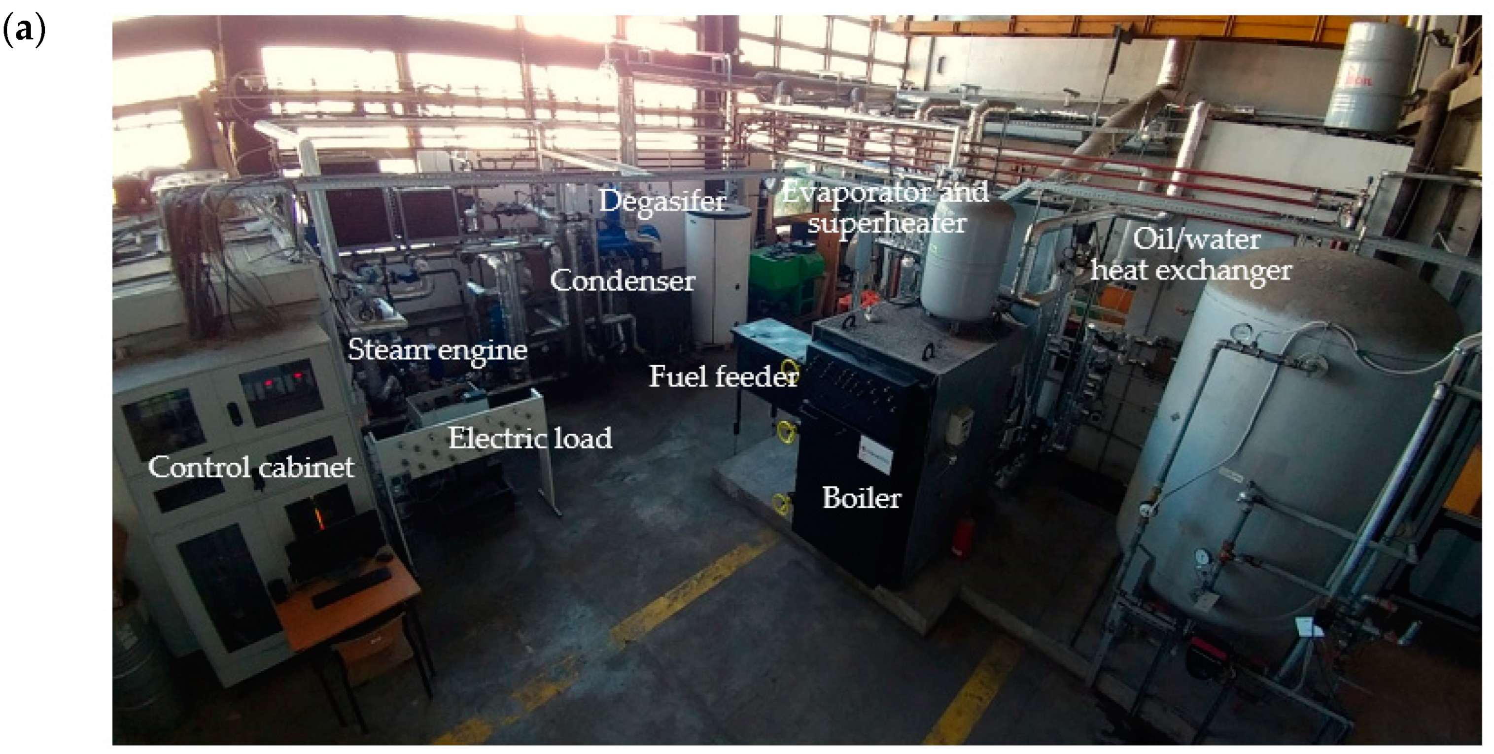
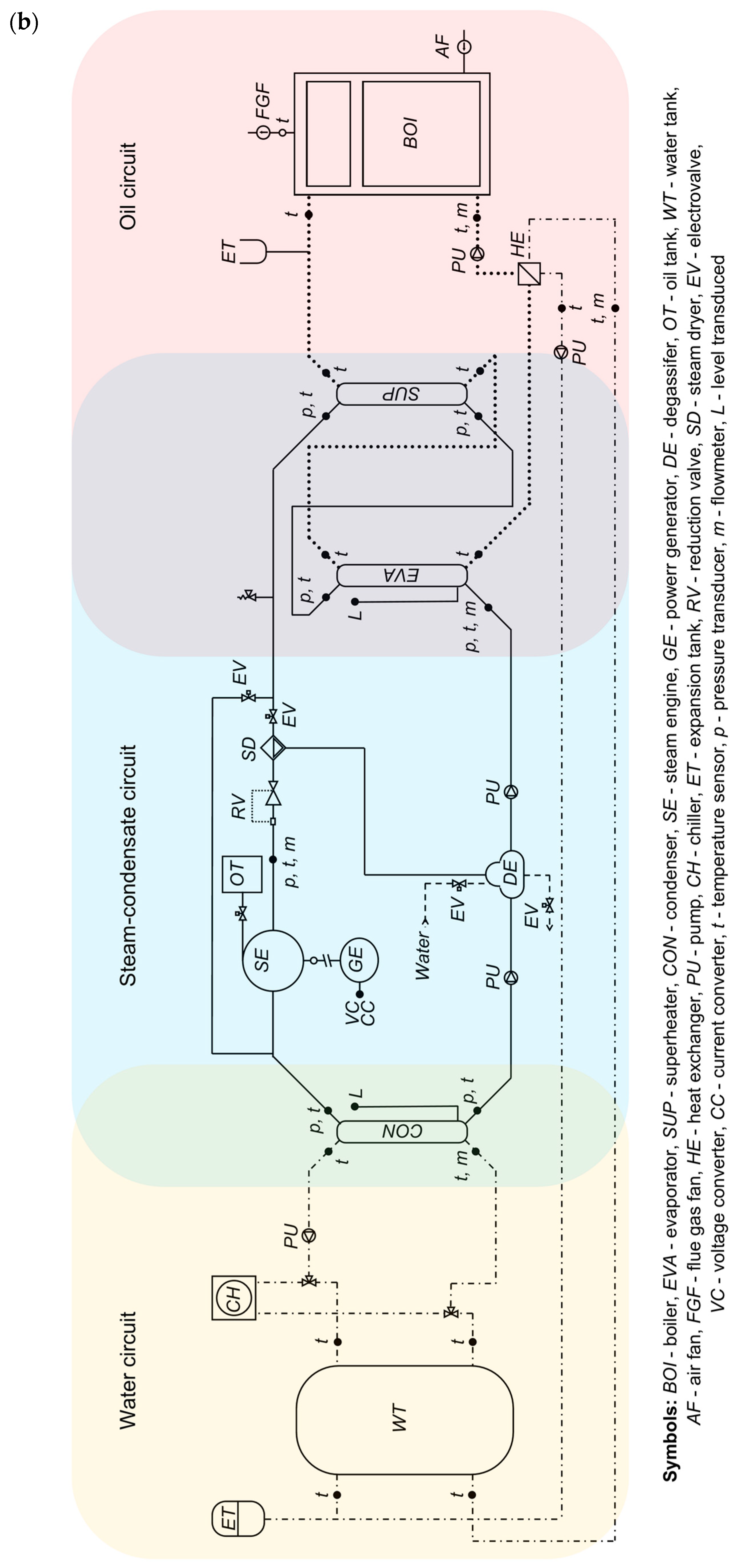
2.1. Construction of the Prototypical System

The analyzed system is divided into three circuits: the thermal oil circuit, the steam–condensate circuit, and the water circuit. In the thermal oil circuit, the oil is heated in a 100 kW_t straw-fired batch boiler. During the presented investigations, Orlen ITERM 6 Mb oil (commonly used in industrial heating and cooling installations) was used. The temperature range of ITERM 6Mb oil is determined by its solidification point, typically −13 °C, and the auto-ignition temperature is typically 252 °C. The density of the oil changes from 906 kg/m³ (0 °C) to 775 kg/m³ (220 °C), while its specific heat changes from 2.1415 kJ/(kgK) to 2.2797 kJ/(kgK), respectively. Hot thermal oil is transferred to shell and tube heat exchangers operating as an evaporator and superheater (shell-and-tube heat exchangers of the JAD type are mostly used in standard industrial installations or heat substations [42]). Moreover, an additional oil-to-water plate heat exchanger was used in the thermal oil circuit, which may be activated when the oil temperature exceeds the upper allowed temperature. Steam generated in the evaporator is then superheated in the superheater and conditioned in the steam dryer and reducing valve. After that process, the steam reaches the expander—double cylinder, acting steam engine V-type 20 hp (the nominal power of the steam engine was declared for the steam pressure of 13.8 bars and the rotation speed of 700 rpm). The engine is connected to a power generator by a belt. Partially expanded steam is condensed in the condenser (shell and tube heat exchanger of JAD type). After condensation, water is pumped to the degasser and the evaporator. The general view and simplified scheme of the system is shown in Figure 1.

The operation of the discussed system €s controlled by a PLC controller equipped with a set of extension modules, measurement elements, and actuators. Among others, the following parameters are measured and recorded by the system:

• Flue gas temperature at the outlet from the boiler;
• Thermal oil temperature (in the selected points) and flow;
• Condensate and steam temperature and pressure (at the selected points);
• The current and voltage generated in the power generator.

The main parameters of the equipment used during the discussed experiments are summarized in

Table 1. The main parameters of the equipment used during the discussed experiments.

Parameter	Equipment	Range	Accuracy
flue gas temperature	K-type (NiCR-Ni) thermocouple sensors	−40–1200 °C	±2.2 °C or ±0.75%
thermal oil temperature	Pt100 resistance sensors	−50–400 °C	tolerance ± 0.3 + 0.005 × [t]
thermal oil flow	ultrasonic flow meter	0–50 kg/h	measuring error up to 2%
condensate and steam temperature	Pt100 resistance sensors	−50–400 °C	tolerance ± 0.3 + 0.005 × [t]
condensate and steam pressure	transducers	0–16 bars
the current generated in the power generator	the current transducers	0–15 A	measuring error lower than ±0.5%
the voltage generated in the power generator	the voltage transducers	0–400 V	measuring error lower than ±0.5%

.

Furthermore, the following parameters are controlled by the PLC controller: inlet air temperature and flow, thermal oil flow, condensate, and steam flow, as well as cooling water flow (via inverters). The parameters mentioned above are available in a visualization created in the CoDeSys software (version 2.3).

2.2. Experimental Procedure

The main goal of the investigations carried out so far was to determine the working parameters of the discussed CHP system, assess the current limitations, and optimize the system configuration (using mathematical modeling).

Table 2. The assumptions for the analyzed series.

Parameter	Series 1	Series 2
The amount of rectangular straw bales in the initializing load	4	4
The amount of additional rectangular straw bales added during the combustion process	9	4
Assumed flue gas temperature at the boiler’s outlet	320–340 °C	320–340 °C
Assumed thermal oil temperature at the boiler’s outlet	190–210 °C	190–210 °C
Assumed pressure of the steam at the superheater’s outlet	8	8
The way of control the condensate pump operation	Continuous control	Two-state control
Electric load setting	Constant	Various

presents assumptions for two measurement series that differed, e.g., in the steam engine operation and a way of controlling the condensate pump operation (continuous and two-state control).

During the described tests, grey straw in the form of rectangular bales was burned. Straw bales were characterized by the weight that ranged from 7 to 13 kg and the average moisture content, which amounted to 17.5% in series 1 and 13.7% in series 2. Depending on the analyzed series, various additional fuel inputs were realized: from 4 to 9. The weight of straw bales fed by the fuel feeder per hour was similar in both series: 45–46 kg/h. Taking into account the average caloric value of the burned straw (ca. 14.4 MJ/kg—value calculated according to data included in [43]), the chemical energy in combusted straw may be estimated at a level of ca. 650–660 MJ/h.

2.3. Retrofitting Optimization of the System

An enhanced thermodynamic model is developed to conduct a retrofitting optimization of the system under examination. First, several technological improvements are set out and applied as one of the modeling assumptions. Then, to examine the system’s operation over a wide range of working conditions, several parameters are introduced (evaporation ratio ER) in this work or adopted (superheating degree SD) from the well-established studies. Next, after defining key equations for the thermodynamic and heat transfer analyses, the optimization problem is formulated. Several constraints are imposed to ensure reliable and technically feasible outcomes. To correctly predict the performance of the modernized system, the geometrical limitations (the heat exchangers stay the same) that keep the calculated heat exchanger areas close to their real values are also included.

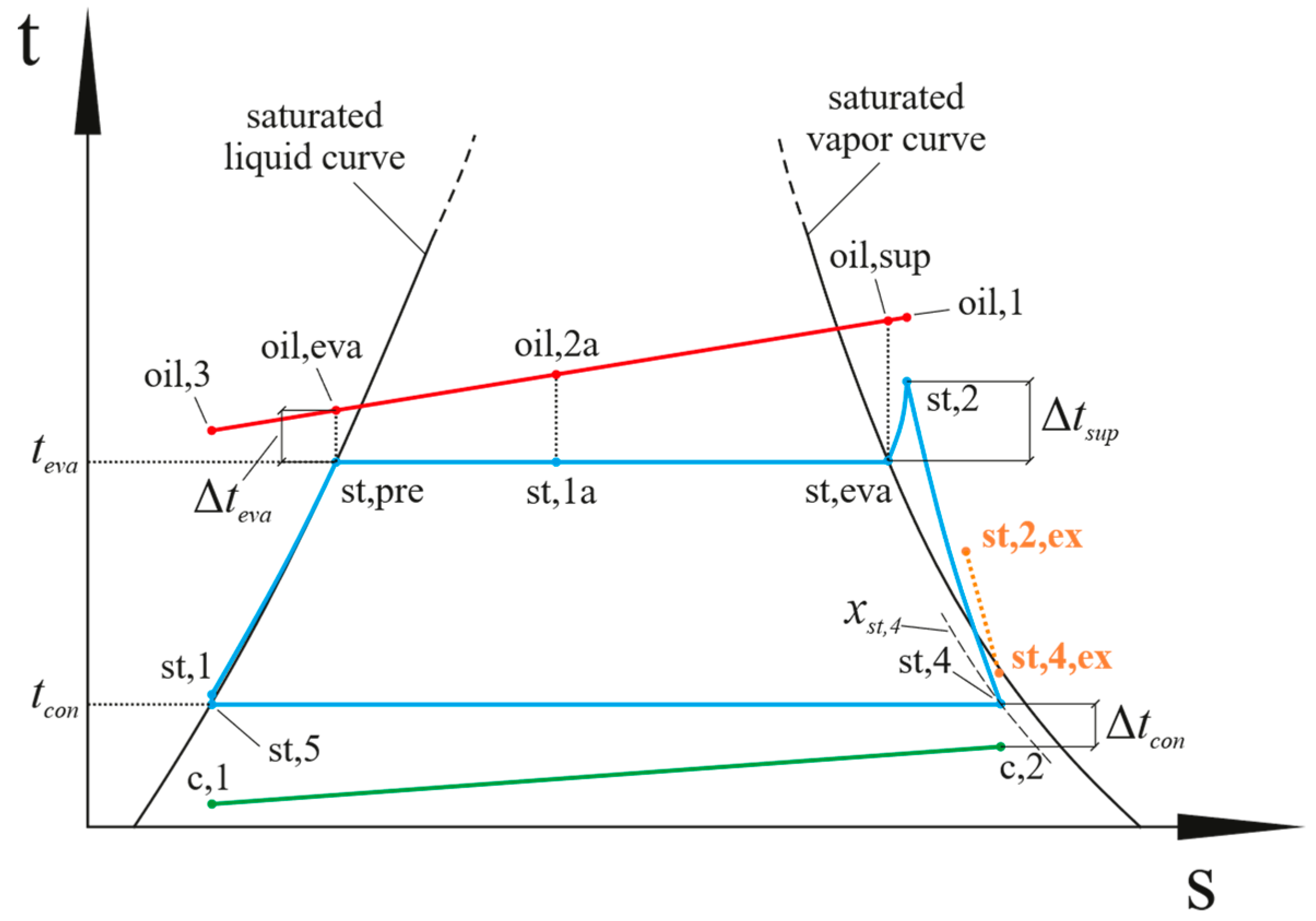
2.4. Thermodynamic Model

To enhance the performance of the system, the following technological improvements are included in the model: (1) the pipes connecting the superheater with the steam engine are well insulated, and their dimensions are lowered so that there are no heat and pressure losses during the flow of the steam, (2) the new power generator with a power capacity of up to 10.0 kW_e is applied, allowing the steam engine to develop higher power output, i.e., >1.50 kW, (3) system automation is introduced providing the system to operate at close-to-steady-state conditions.

In addition, to simplify modeling of the system, the following assumptions were made: (1) there are no heat and pressure losses in the heat exchangers and all connecting pipes, (2) the piston engine operates with a constant isentropic efficiency of η_i,PE = 0.50 [44], (3) the pump operates with the efficiency of η_i,P = 0.75 [45], (4) the kinetic and potential energy changes of the fluids are neglected.

Based on the abovementioned assumptions, the system should operate according to the thermodynamic cycle depicted in Figure 2. In the same figure, simplified temperature distributions of the heat carrier (thermal oil) and heat sink (cooling water) are illustrated as well. Water that implements the depicted thermodynamic cycle undergoes the following thermodynamic processes:

• Isobaric preheating (st,1–st-pre), evaporation (st,pre–st,eva), and superheating (st,eva–st,2) in the heat exchangers (“evaporator” and “superheater”);
• Irreversible expansion (st,2–st,4) in the steam engine;
• Isobaric condensation (st,4–st,5) in the condenser;
• Irreversible pressurizing (st,5–st,1) of the fluid in the pump.

In Figure 2, there is also an approximate illustration of the expansion process (st,2,ex–st,4,ex) that takes place in the existing, non-optimized installation state. Due to the partial expansion of the steam in the pipes connecting the superheater with the engine, the ideal state st,2 is shifted to st,2,ex. This effect and the higher steam pressure at the engine outlet substantially reduce the engine’s pressure ratio, thus decreasing the engine power outputs. The latter aspect is further discussed in Section 3.

While creating a thermodynamic model of the system, each component (or subcomponent covering a certain process) is considered a control volume. The unknown thermodynamic quantities, including heat transferred by the water in the individual processes, the power output of the piston engine, or power consumed by a pump, are determined with the use of mass (Equation (1)) and energy (Equation (2)) balance equations:

$$\sum {\dot{m}}_{in}=\sum {\dot{m}}_{out}$$

(1)

$$\sum {\dot{m}}_{in}{h}_{in}+\dot{Q}=\sum {\dot{m}}_{out}{h}_{out}+P_{out}$$

(2)

As mentioned in the previous sections, the evaporation process of the steam takes place partially in the “superheater”, which results from an insufficient heat transfer area of the “evaporator” (the names of these heat exchangers are given in quotes throughout this section since in the current configuration of the system, they do not work according to their original purpose). For this reason, at the outlet of the “superheater”, the thermal oil is cooled down to the temperature t_oil,2a, which is lower than the temperature t_oil,sup required to accomplish the superheating process (see Figure 2). Therefore, the specific value of t_oil,2a depends on the extent to which the steam is evaporated in the “superheater”. To include this phenomenon in the model, the evaporation ratio (ER) indicator is proposed in this study, and it is formulated as follows:

$$ER=\frac{{\dot{Q}}_{eva,sup}}{{\dot{Q}}_{eva}}=\frac{{\dot{m}}_{oil}{c}_{oil}\left(t_{oil,sup}-t_{oil,2a}\right)}{{\dot{m}}_{oil}{c}_{oil}\left(t_{oil,sup}-t_{oil,eva}\right)}$$

(3)

As seen in Equation (3), ER is defined as the ratio of the heat transferred during the evaporation of the steam in the “superheater” to the heat required for completing the evaporation of this fluid. The physical meaning of ER can be described by considering its limiting values, i.e., 0.00 and 1.00. For ER = 0.00, no evaporation heat is transferred in the “superheater”, while for ER = 1.00, the entire evaporation process is accomplished in the “superheater”.

A key parameter to be distinguished in the modeling of the Rankine cycle is the degree of superheating. In Figure 2, it is represented by Δt_sup that is defined as the difference between the temperature of the steam at state st,2 and the temperature of the steam at state st,eva. Apart from its impact on the power output and thermal efficiency of the cycle, Δt_sup also determines the state of the steam at the outlet of the piston engine. The latter aspect can be expressed by the steam quality x_st,4 (see Figure 2), the value of which should be kept above a certain level to avoid excessive formation of the water droplets. By recalling the superheating degree parameter (SD) applied in the study by Chatzopoulou et al. [46], the degree of superheating can be formulated as follows:

$$SD=\frac{∆t_{sup}}{t_{oil,1}-\left[∆t_{pinch,min}+t_{eva}\right]}$$

(4)

where Δt_pinch,min is the minimum allowable temperature difference between the thermal oil and water across the heat exchangers, and its assumed value is equal to 3.00 K. The SD parameter allows conveniently specifying a maximum possible superheating of the steam under given values of the evaporation temperature t_eva and the temperature of the heat carrier t_oil,1. Specifically, for SD = 1.00, the oil temperature t_oil,1 differs from the steam temperature t_st,2 by the minimum limit value. Meanwhile, for SD = 0.00, there is no superheating of the steam, and its state st,2 corresponds to the point that lies on the saturated vapor curve, i.e., the point marked as st,eva.

Another parameter substantially affecting the system performance is the difference Δt_eva between the heat carrier temperature t_oil,eva and the water temperature t_st,pre at the saturated liquid point (see Figure 2). By adopting the nomenclature given in Figure 2, this parameter can be formulated as follows:

$$∆t_{eva}=t_{oil,eva}-t_{eva}$$

(5)

Many scholars have shown that Δt_eva affects both thermodynamic performance [47] (via an impact on the net power output) and economic viability [48] (via an influence on the heat exchanger area). Even though the economic aspect is not an issue in this study (the model is built for an existing system with a predefined heat exchangers size), an impact on the heat transfer area is still crucial since it is one of the deciding factors in determining the feasible working conditions of the system.

The thermodynamic parameters of the evaporation t_eva and condensation t_con temperatures of the steam (marked in Figure 2) strongly affect the thermal efficiency of the SRC. Hence, they are also key for improving the performance of the entire SRC installation.

As one of the most significant performance indicators of the power plant capacity, the electrical power output of the piston engine is examined in this study. It is determined using the following equation:

$$P_{el}={\eta }_m{\eta }_{el}{\dot{m}}_{st}\left(h_{st,2}-h_{st,4}\right)$$

(6)

The mechanical η_m and electrical η_el efficiency are assumed to be equal to 85% and 95% [49], respectively. The specific enthalpy h_st,4 is calculated by applying definition of the isentropic efficiency of the piston engine:

$${\eta }_{i,PE}=\frac{h_{st,2}-h_{st,4}}{h_{st,2}-h_{st,4s}}$$

(7)

Apart from electricity production, the considered system is designed to supply the heat through the condensation process st,4–st,5. To evaluate the cogeneration performance of the Rankine cycle, the energy utilization factor ε_R is determined using the following equation:

$${\epsilon }_R=\frac{P_{net}+{\dot{Q}}_{con}}{{\dot{Q}}_{eva}}·100\mathrm{\%}$$

(8)

The net power output P_net is calculated as the difference between the electric power of the piston engine and the power consumed by the pump:

$$P_{net}=P_{el}-P_P$$

(9)

The power consumption of the pump is calculated as:

$$P_P={\dot{m}}_{st}\left(h_{st,1}-h_{st,5}\right)$$

(10)

As with determining the specific enthalpy h_st,4 at the outlet of the piston engine, the specific enthalpy h_st,1 at the outlet of the pump is computed with the use of isentropic efficiency of the pump:

$${\eta }_{i,P}=\frac{h_{st,1s}-h_{st,5}}{h_{st,1}-h_{st,5}}$$

(11)

The heat transferred during the evaporation and condensation processes are calculated from the following relationships:

$${\dot{Q}}_{eva}={\dot{m}}_{st}\left(h_{st,2}-h_{st,1}\right)$$

(12)

$${\dot{Q}}_{con}={\dot{m}}_{st}\left(h_{st,4}-h_{st,5}\right)$$

(13)

In the case of the SRC, the power consumed by the pump is usually negligible when compared to the power generated by the expander [50]. To verify this statement for the examined installation, the ratio RCG between the consumed and generated power of the cycle is calculated using the following equation:

$$RCG=\frac{P_P}{P_{el}}·100\%$$

(14)

The thermodynamic analysis is complemented by determining the thermal efficiency of the Rankine cycle:

$${\eta }_R=\frac{{\dot{m}}_{st}\left[\left(h_{st,2}-h_{st,4}\right)-\left(h_{st,1}-h_{st,5}\right)\right]}{{\dot{Q}}_{eva}}·100\%$$

(15)

2.5. Heat Transfer Analysis

The simplified heat transfer model is constructed to estimate the overall heat transfer coefficients k for the heat exchangers and to calculate the heat exchangers’ heat transfer areas. The overall heat transfer coefficients are estimated based on their mean values (see

Table 3. Constant parameters for conducting optimization procedure.

toil,1 [°C]	${\dot{V}}_{oil}$ [L min−1]	tc,1 [°C]	Δtcon [K]	Δtpinch,min [K]	ηi,PE [%]	ηm [%]	ηel [%]
210	46.3	20.0	10.0	3.00	50	85	95
ηi,P [%]	kpre [W m−2 K−1]	keva [W m−2 K−1]	ksup [W m−2 K−1]	kcon [W m−2 K−1]	AE,real [m2]	AS,real [m2]	ACON,real [m2]
75	300	567	35.6	485	5.10	5.10	10.7

) that are calculated for the selected experimental data points (the time interval between 95.0 min and 100 min was selected—see Figure 3). Meanwhile, the heat transfer areas are determined while conducting retrofitting optimization of the system (see Section 2.8). For both procedures, i.e., for determining coefficients k and heat transfer areas A, the logarithmic mean temperature difference (LMTD) method is employed. The equations corresponding to the individual heat exchangers and their sections are given below.

• “Evaporator”

The “evaporator” is divided into sections in which the processes of preheating and evaporation are conducted. It is worth noting that evaporation occurs in the “evaporator” and “superheater”. Therefore, the LMTD equations corresponding to the preheating and evaporation processes in the “evaporator” are as follows:

$$A_{pre}=\frac{{\dot{Q}}_{pre}}{k_{pre}∆t_{log,pre}}$$

(16)

$$A_{eva,E}=\frac{{\dot{Q}}_{eva,E}}{k_{eva}∆t_{log,eva,E}}$$

(17)

$$A_E=A_{pre}+A_{eva,E}$$

(18)

• “Superheater”

In the “superheater”, the evaporation process of the steam is completed, and then the superheating process of the saturated steam takes place. Thereby, the applied equations for the individual sections of the “superheater” (subscript S) can be written as:

$$A_{eva,S}=\frac{{\dot{Q}}_{eva,S}}{k_{eva}∆t_{log,eva,S}}$$

(19)

$$A_{sup}=\frac{{\dot{Q}}_{sup}}{k_{sup}∆t_{log,sup}}$$

(20)

$$A_S=A_{eva,S}+A_{sup}$$

(21)

• “Condenser”

In the condenser (subscript CON), only two-phase condensation of the steam takes place, and hence, the heat transfer equation can be written in the following form:

$$A_{CON}=\frac{{\dot{Q}}_{con}}{k_{con}∆t_{log,con}}$$

(22)

The fluids flow counter-currently in the heat exchangers. Accordingly, the general formula for the logarithmic mean temperature difference can be written as follows:

$$∆t_{log}=\frac{\left(t_{hot,in}-t_{cool,out}\right)-\left(t_{hot,out}-t_{cool,in}\right)}{ln\frac{\left(t_{hot,in}-t_{cool,out}\right)}{\left(t_{hot,out}-t_{cool,in}\right)}}$$

(23)

where the subscripts hot and cool refer to the hot and cool medium, while the subscripts in and out pertain to the inlet and outlet state of the fluid.

2.6. Input Parameters

The parameters that are constant during the optimization procedure are listed in Table 3. As indicated in Table 1, the temperature range of the thermal oil during the measurement series is between 190 °C and 210 °C. To assess the system’s maximum performance, the upper bound of that range is taken as the inlet thermal oil temperature t_oil,1. Since there were little variations in the volume flow rate of the thermal oil ${\dot{V}}_{oil}$, it was decided to calculate its mean value, relying on the measurement data encompassing the time interval of 95.0–100 min. The cooling water at the inlet to the condenser is set at the ambient temperature of 20.0 °C. The temperature difference Δt_con (see Figure 2) is assumed to be equal to 10.0 K, similarly as in [51].

2.7. Validation of the Model

The validation of the thermodynamic model applied in this study was shown in detail in [48], and therefore it is not presented herein.

2.8. Optimization Problem

As mentioned previously, the retrofitting optimization of the steam cycle is aimed at maximizing the electrical power output of the system. Thereby, the electrical power P_el is selected as the criterion to be optimized, and the genetic algorithm (GA) is employed as a tool to find the optimal operating conditions of the system. The parameters that are selected as decision variables include the following: (1) evaporation temperature t_eva, (2) superheating degree parameter SD, (3) temperature difference Δt_eva, (4) condensation temperature t_con, and (5) evaporation ratio ER. The single-objective optimization that aims to find the optimal value of P_el is formulated as follows:

$$\underset{\overrightarrow{X}}{\min }f\left(\overrightarrow{X}\right)=-P_{el}$$

(24)

subject to

$$t_{eva}\ge t_{con}$$

(25)

$$0\le SD\le 1$$

(26)

$$∆t_{pinch,min}\le ∆t_{eva}\le 20.0\mathrm{K}$$

(27)

$$0\le ER\le 1$$

(28)

$$x_{st,4}\ge 0.90$$

(29)

$$∆t_{pinch,HX}\ge ∆t_{pinch,min}$$

(30)

$$\frac{\left|A_E-A_{E,real}\right|}{A_{E,real}}\le 0.05$$

(31)

$$\frac{\left|A_S-A_{S,real}\right|}{A_{S,real}}\le 0.05$$

(32)

$$\frac{\left|A_{CON}-A_{CON,real}\right|}{A_{CON,real}}\le 0.05$$

(33)

The vector of decision variables $\overrightarrow{X}$ can be written as:

$$\overrightarrow{X}={\left[t_{oil,1},t_{eva},SD,∆t_{eva},t_{con},ER\right]}^T$$

(34)

To obtain technically feasible solutions to the problem defined in Equation (24), the constraints given in Equations (25)–(30) are imposed on the selected thermodynamic and heat transfer parameters. By imposing the constraint given in Equation (25), the non-feasible configurations of the Rankine cycle are excluded. The superheating degree SD and evaporation ratio ER are parameters defined in a range between 0.00 and 1.00, which is considered in the constraints presented in Equations (26) and (28). The temperature difference Δt_eva is limited (Equation (27)) similarly as in [47]. The limitation imposed on the steam quality (Equation (29)) allows avoiding excessive formation of the water droplets at the end of the expansion process in the piston engine. The pinch point temperature difference Δt_pinch,HX (i.e., the smallest temperature difference between the fluids across the heat exchanger) is always greater than Δt_pinch,min (Equation (30)) to exclude infeasible heat transfer conditions.

Since the optimization is performed for an existing system with a predefined heat exchangers size (the values of A_S,real, A_E,real and A_CON,real are given in Table 3), the calculated heat transfer areas of the “evaporator”, “superheater” and condenser should not deviate from their real values by more than 5.00%, which is expressed in Equations (31)–(33).

3. Results and Discussion

The energy flow in the boiler and oil circuit was analyzed at the beginning of the presented investigation. Data in

Table 4. Energy flow in the boiler and oil circuit.

Series No.	The Heat Generated in the Boiler and Transferred to the Oil MJ	Heat Transferred from Oil to Condensate and Steam MJ	Heat Transferred from Oil to Water MJ	Heat Losses in Pipes and Fittings MJ
1	721.4 ± 14.6	458.8 ± 9.3	200.3 ± 4.1	62.3 ± 1.3
2	574.6 ± 11.6	314.1 ± 6.4	233.2 ± 4.7	27.3 ± 0.5

show that more than 50% of the heat generated in the boiler was transferred from oil to condensate and steam in the evaporator and superheater (63.6% and 54.7%, respectively). Heat losses in the pipes and fittings were quite high—from 4.8% (series 2) to 8.6% (series 1). The uncertainties of energy values were calculated using the root sum of the squares.

On the other hand, taking into account the chemical energy contained in the straw inputs and the amount of heat generated in the boiler, its efficiency was quite low—ca. 51.7% and ca. 47.3% during series 1 and 2, respectively (compared to the nominal value of 82% given by manufacturer). Such low boiler efficiency resulted, e.g., from the combustion process starting on a cold boiler, working with a chimney draft up to 3–4 times higher compared to typical water units (high chimney draft was required to provide an assumed oil temperature at the outlet from the boiler), as well as from the manual control of the system operation.

3.1. The Steam Temperature and Pressure at the Outlet from the Superheater

The comparison of steam temperature and pressure variations at the outlet from the superheater during series 1 and series 2 is shown in Figure 3. In both series, the maximum steam temperature was ca. 200 °C (it was reached in the 9^0th minute). During the operation of the steam engine, the average steam temperature was ca. 185–190 °C. During series 1, the maximum steam pressure of 8.5 bar was reached in the 6^0th minute, while in series 2, the maximum steam pressure of 7.5 bar was observed in the 7^5th minute. In both cases, after opening the reduction valve, the pressure in the steam–condensate circuit was lowered due to the partial expansion of the steam in the pipeline. As a result, the average steam pressure at the superheater outlet during steam engine operation was, respectively, ca. 5 bars during series 1 and ca. 4 bars during series 2. The variations in the steam pressure were related to, among others, the current setting of the reduction valve, the set of electric loads connected to the steam engine, and the way the operation of the condensate pump was controlled.

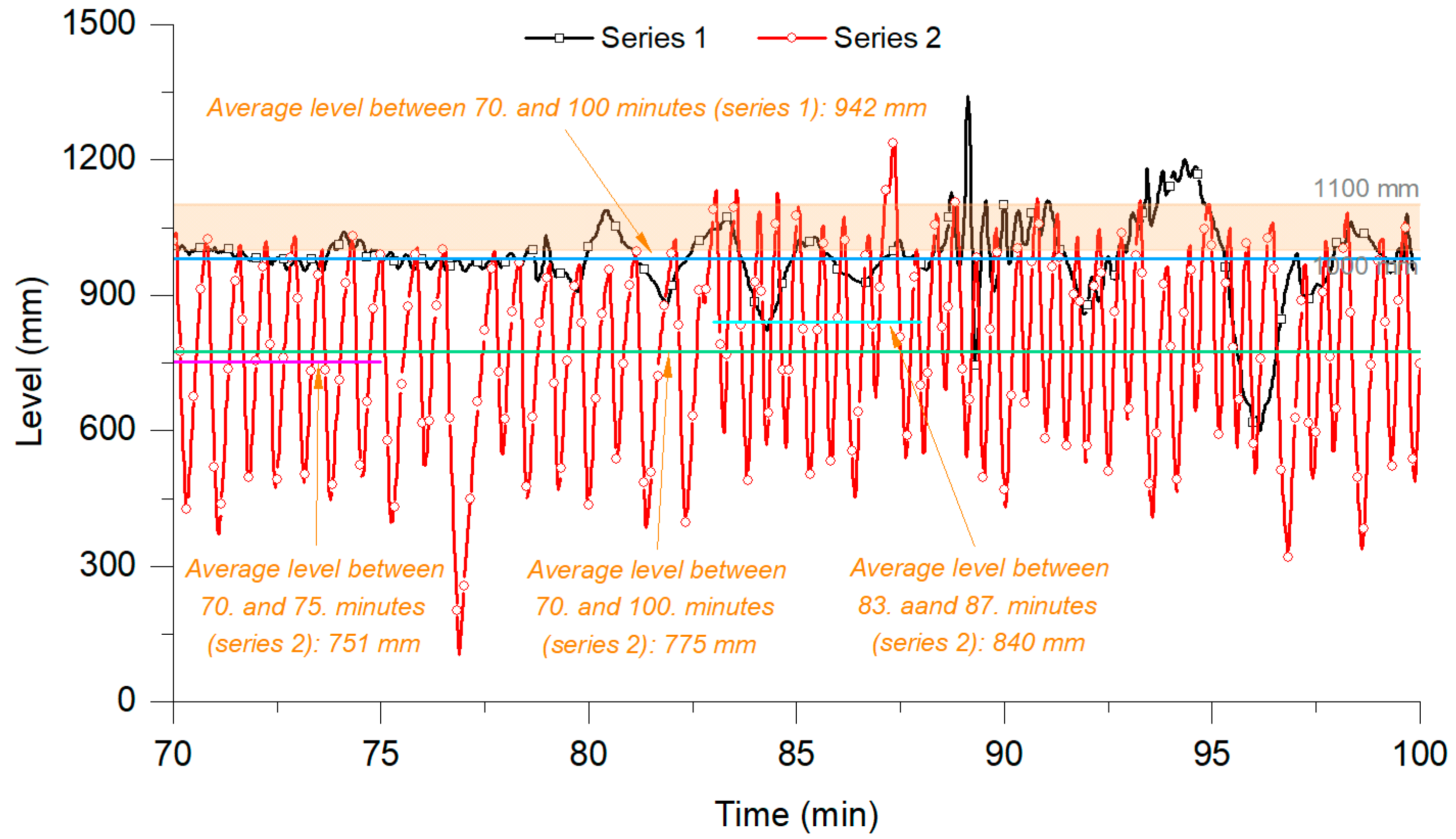
3.2. A Comparison of Continuous and Two-State Control of Condensate Pump Operation

Steam parameters at the superheater outlet depended on different factors, including the reducing valve set, steam engine operation (including electric load set), and condensate pump operation. Two different ways of controlling the condensate pump operation were analyzed during series 1 and 2. The level of water in the evaporator was assumed to be 1000 mm. In the case of series 1, the water level in the evaporator was controlled by continuously adjusting the setting of the condensate pump via the inverter. The average water level in the evaporator was ca. 933 mm. On the other hand, during series 2, the two-state control method was tested. Each time the water level exceeded the assumed value, the condensate pump was switched on for 10–30 s (the exact time was determined by the water level). To illustrate the differences in the water level variations in the evaporator during series 1 and series 2, the time between 70 and 100 min was tested, as presented in Figure 4. In the case of continuous control (series 1), the average water level in the evaporator was equal to 942 mm, while in the case of two-state control (series 2), the average water level in the evaporator was significantly lower—equal to 775 mm. On the other hand, it depended on the selection of signaling levels. During series 2, the average water level was 751 mm between the 7^0th and 7^5th minutes (when the pump was turned off when the water level reached 1000 mm) and 840 mm between the 8^3rd and 8^7th minutes (when the pump was turned off when the water level reached 1100 mm).

3.3. The Efficiency of the Evaporator and Superheater

The heat required for the evaporation of water in the evaporator and superheating of steam in the superheater was calculated for the time between the 7^5th and 8^5th minutes. The calculated values were compared with the amount of heat received from the oil. The efficiency of evaporation and superheating processes was determined. The results (along with the boundary conditions) are presented in

Table 5. The efficiency of the evaporator and superheater during series 2 (between 7^5th and 8^5th minutes).

Position	Evaporator	Superheater
The average temperature at the inlet to the heat exchanger [°C]	55.0	168.7
The average temperature at the outlet from the heat exchanger [°C]	168.7	187.4
The average pressure in the heat exchanger area (on the steam–condensate side) [bar]	6.8	6.7
Amount of condensate/steam [kg]	55.0	55.0
The amount of heat received from the oil [kWh]	8.67	2.63
The amount of heat transferred to the condensate/steam [kWh]	6.43	0.12
The average power in relation to the heat exchange surface [kW/m2]	9.8	3.0
Heat exchanger efficiency [%]	74.2	4.5

. The average superheater power related to its surface was over three times lower than that of the evaporator. Moreover, the efficiency of the superheater was almost 17 times lower than the evaporator efficiency (it was caused, e.g., by the fact that condensate was partially evaporated in the superheater area, which was not included in the calculations). On the other hand, in the next version of the micro-cogeneration system (version ready to test in real conditions before its final commercialization), the size of the superheater should be limited. As previously calculated, the required superheater size is lower than the evaporator. The currently installed superheater is oversized because its function may be switched to the evaporator (shell and tube heat exchangers are connected in series now, but they may also be connected in parallel).

3.4. Condensate and Steam Temperature Distribution in the Steam–Condensate Circuit

Condensate and steam temperature distribution in the steam–condensate circuit were analyzed during series 2. The electric load was set during tests to determine the operating characteristics of the power generator. The average steam temperature in the main phase of the system operation was measured as 151.7 °C, 171.6 °C, and 123.5 °C at the evaporator outlet, the superheater outlet, and the steam engine inlet, respectively. The average steam temperature drop in the pipeline between the superheater and the steam engine was, therefore, 48.1 K (compared to 52.8 K in the case of series 1). Such a significant decrease in the steam temperature resulted mainly from the large pipe volume (and consequently reduced steam velocity), the too-small thickness of the pipes’ thermal insulation (only 30 mm of mineral wool), and heat losses on partially uninsulated valves and other components. Moreover, during the described tests, all installation run-ups were performed from a cold state, so a part of the heat transferred from the oil to condensate, and steam was used to preheat steam/condensate circuit components (in the initial phase of the steam/condensate circuit operation). Variations in the condensate temperature were caused by way of controlling its level in the evaporator (two-state control strategy during series 2). The variations in the steam and condensate temperatures in the steam–condensate circuit when the steam engine operated during series 2 are shown in Figure 5.

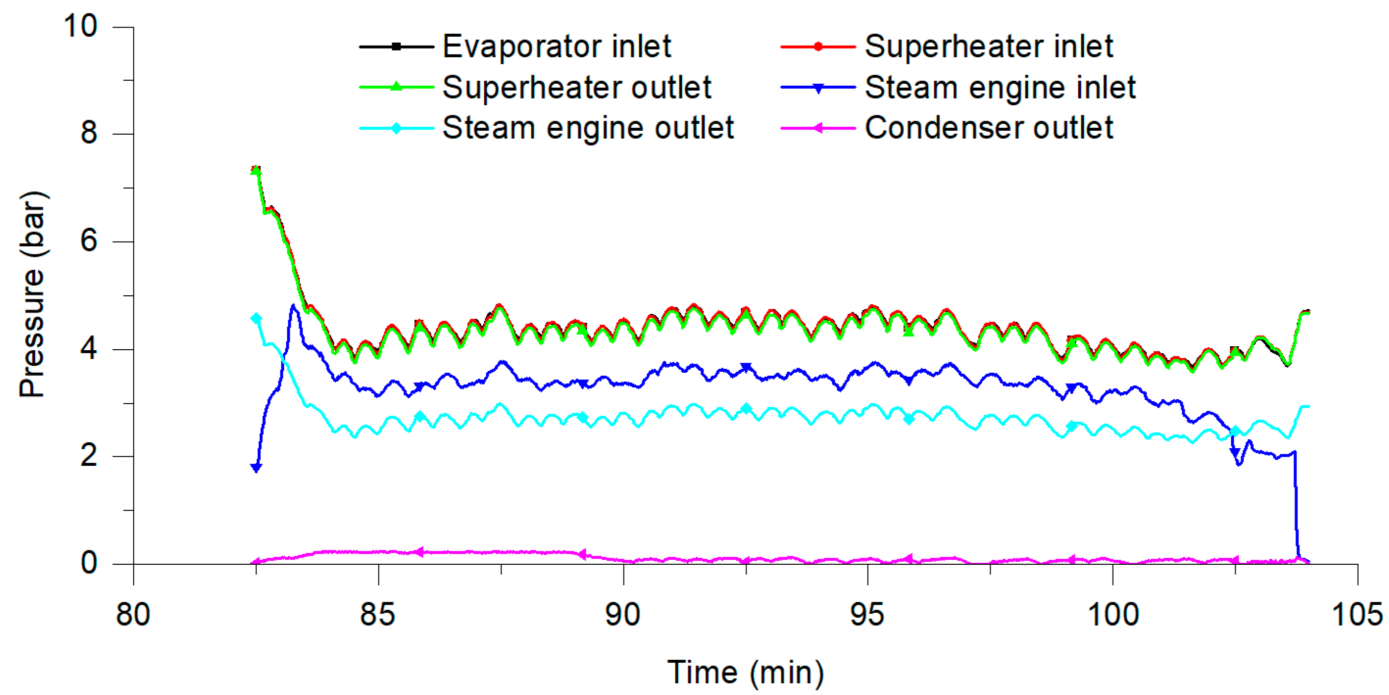
3.5. Condensate and Steam Pressure Distribution in the Steam–Condensate Circuit

During series 2, the reduction valve was opened in the 3^5th minute of the combustion process (the beginning of the main phase). Up to the 7^5th minute, steam flowed through the bypass (the steam engine was switched off). Hence, there was a gradual increase in pressure in the individual parts of the steam–condensate circuit for this series. As the reference point, the pressure at the superheater outlet was chosen. After reaching the level of 7.0 bars, the steam engine was switched on, and after reaching the level of 7.5 bars, the set of reduction valve was changed from 30% to 80%. Modification of the reducing valve setting caused an increase in the steam flow and a significant drop in the steam pressure at the superheater outlet (from 7.5 to 4.0 bars). Then, between 84 and 103 min, steam pressure at the superheater outlet was maintained at an average level of 4.3 bars. At the same time, the average steam pressure at the inlet of the steam engine was only 3.3 bars, and the average steam pressure at the inlet of the condenser was 2.7 bars (see Figure 6).

3.6. Steam Temperature and Pressure Variations in the Steam Pipeline

The main problem from the standpoint of the steam–condensate circuit operation is a significant drop in temperature and pressure.

Table 6. Temperature and pressure variations in the selected parts of the steam–condensate circuit.

Element	Pressure Variations, Bars	Temperature Variations, K
Evaporator and superheater	−0.07	+151.3
Pipeline between superheater and steam engine	−0.89	−52.3
Steam engine	−0.71	−46.5

shows steam temperature and pressure changes in the evaporator and superheater, the pipeline between the superheater outlet and steam engine inlet, and the steam engine (during series 2). The highest pressure drop (0.89 bar) was observed in the pipeline between the superheater and the steam engine (approximately 0.06 bar/m). The pressure drop in the pipeline was greater than in the steam engine. This situation was caused mainly by the steam cooling in the pipeline (a temperature drop of 52.3 K) and local pressure losses on the elbows, valves, and other elements.

3.7. Operating Characteristics of the Power Generator

The power generated in the power generator resulted from the actual steam parameters (pressure, flow, temperature) and the setting of the electric load. During this process, maximum power point tracking was realized by changing the settings of the electric load from 0 to 2.0 kW_e. The maximum power was approx. 1.15 kW_e, and it was achieved when thermal power generated in the boiler was observed at the level of approx. 110 kW_t. Consequently, the share of electricity generation in the total energy generation was only 1.05%. Such low power resulted mainly from a very low power generator capacity (simple construction of the generator with a maximum power of ca. 1.5 kW_e was used at the current stage). Other limitations were also caused by a low steam inlet pressure (a consequence of limitations in the oil and steam temperature and steam bus construction, including, e.g., large pipe capacity) or too-large steam pressure at the engine outlet.

3.8. Optimization Results

The results of the optimization procedure are listed in

Table 7. Results of a single-objective optimization.

Decision Variables					Objective Function
teva [°C]	SD [-]	Δteva [K]	tcon [°C]	ER [-]	Pel [kWe]
143	0.80	3.00	46.4	0.56	9.03

. As seen, the optimized value of the electrical power output of the system is equal to 9.03 kW_e. For a more complete picture of the relation between the power output P_el and individual decision variables, a parametric analysis was conducted, and its findings are presented in Figure 7.

A peak value (~10 kW_e) of the power output P_el is observed in Figure 7a, in which the influence of the evaporation temperature t_eva is examined. It is noted that the optimized value of t_eva (143 °C) is higher than t_eva corresponding to the point of maximum power output. The inability to obtain the highest value of P_el is related to severe constraints (particularly those related to heat transfer areas) imposed on the system parameters. For example, the values of t_eva lower than 143 °C correspond to higher mass flow rates of the steam (due to lower heat required for the preheating and evaporation of the water), which results in unacceptably high heat transfer areas.

As shown in Figure 7b, the superheating degree SD parameter slightly affects the power output P_el. However, SD plays a key role in satisfying constraints defined in Equation (32) since it affects the heat transfer area of the “superheater”.

In the case of the temperature difference Δt_eva and the condensation temperature t_con that are examined in Figure 7c,d, similar trends can be observed. For both parameters, their lower values are associated with higher power outputs P_el, which is reflected in the optimal solutions listed in Table 7.

As shown in Figure 7e, the evaporation ratio ER does not affect the power output P_el of the system. However, as a parameter which determines the heat distribution between the “evaporator” and “superheater”, it allows finding a number of feasible solutions under different working conditions of the system. In other words, by applying ER in the optimization procedure, a more flexible selection of the operating parameters is provided and, thereby, higher power outputs of the SRC installation can be found.

The optimized values of the remaining performance indicators that were considered within the frame of thermodynamic analysis are listed in

Table 8. Performance indicators corresponding to optimal working conditions of the System.

${\dot{\mathit{Q}}}_{\mathit{e}\mathit{v}\mathit{a}}$ [kW]	${\dot{\mathit{Q}}}_{\mathit{c}\mathit{o}\mathit{n}}$ [kW]	PP [kW]	Pnet [kW]	RCG [%]	εR [%]	ηR [%]
103	91.4	0.02	9.01	0.22	97.9	10.9

. Compared to the existing installation, the retrofitted SRC system features an increased electrical power output P_net (9.01 kW_e compared to 1.15 kW_e) and improved thermal cycle efficiency η_R (10.9% compared to 1.05%). After optimizing its performance, the SRC installation also exhibits excellent energy utilization factor ε_R of about 98%. It is worth noting that this result is similar to that achieved (93.0%) for the highly efficient micro-CHP installation based on the ORC technology [30].

As anticipated, the power consumption of the pump accounts for a very small fraction of the piston engine power, which is reflected in a low value of the RCG ratio (0.22%). For comparison, in the micro-CHP systems that operate with other working mediums (hydrocarbons, refrigerants), such a low power requirement is practically unattainable, and the RCG ratio may reach the value of even more than 20.0% [51].

Even though the findings which are summarized in Table 8 are based on the optimization procedure and have not yet been experimentally recreated, they indicate the strong potential of the examined system after introducing the previously mentioned improvements. The experimental verification of an upgraded configuration of the installation will be addressed in future studies.

4. Conclusions

The prototype of the micro-CHP system with a straw-fired boiler and modified Rankine cycle was briefly characterized and tested. An experimental analysis of the selected steam–condensate circuit was conducted, including a comparison of two control scenarios, the condensate level in the evaporator, steam temperature, and steam pressure variations, as well as the operating characteristics of the power generator. The main findings resulting from the carried-out investigations are as follows:

• The use of continuous control of condensate pump operation allowed providing a more stable condensate level in the evaporator. Between the 70^th and 100^th minutes of the combustion process, the average water level was 942 mm in the case of a continuous control and 775 mm in the case of a two-state control.
• In the considered time, the average superheater power related to its surface was over three times lower compared to the evaporator, and the efficiency of the superheater was calculated to be ca. 17 times lower than the evaporator efficiency.
• Significant drops in the steam temperature and pressure were observed in the pipeline between the superheater outlet and steam engine inlet: 52.3 K and 0.89 bar, respectively.
• The maximum obtained electrical power was only ca. 1.15 kW_e. The main reason for such a low value was a very low power generator capacity, but other limitations were caused also by low steam pressure (which was a consequence of limitations in oil and steam temperature and steam bus construction, including large pipe capacity). Based on the observed system limitations, the required modifications were listed.
• Based on the suggested technological improvements, an original thermodynamic model incorporating new (evaporation ratio, ER) and well-established (superheating degree, SD) parameters was developed. Making use of the model, a retrofitting optimization of the system was conducted.
• The results of a retrofitting optimization of the system show that the electrical power output may be as high as 9.0 kW_e.
• At the optimal operating conditions, the studied system was characterized by an energy utilization factor of 97.9%.

Overall, it was demonstrated that the small-scale SRC has potential to serve as an alternative technology for micro- and distributed cogeneration systems. Being a technology that can be supplied with renewable biomass energy, and that is based on a cheap and environmentally friendly working medium (water), it perfectly fits into the idea of sustainable development of energy systems, and hence, it should be further promoted.

References

1. Ventura, C.; Wu, Q. Theoretical Evaluation of Photovoltaic Thermal Water Source Heat Pump, Application Potential and Policy Implications: Evidence from Yangtze River Economic Belt, China. Sustainability 2023, 15, 13638. [Google Scholar] [CrossRef]
2. Energy Statistics—An Overview—Statistics Explained. Available online: https://ec.europa.eu/eurostat/statistics-explained/index.php?title=Energy_statistics_-_an_overview#Final_energy_consumption (accessed on 29 October 2023).
3. Delgado-Plaza, E.; Carrillo, A.; Valdés, H.; Odobez, N.; Peralta-Jaramillo, J.; Jaramillo, D.; Reinoso-Tigre, J.; Nuñez, V.; Garcia, J.; Reyes-Plascencia, C.; et al. Key Processes for the Energy Use of Biomass in Rural Sectors of Latin America. Sustainability 2022, 15, 169. [Google Scholar] [CrossRef]
4. Koval, V.; Laktionova, O.; Udovychenko, I.; Olczak, P.; Palii, S.; Prystupa, L. Environmental Taxation Assessment on Clean Technologies Reducing Carbon Emissions Cost-Effectively. Sustainability 2022, 14, 14044. [Google Scholar] [CrossRef]
5. Tshikovhi, A.; Motaung, T.E. Technologies and Innovations for Biomass Energy Production. Sustainability 2023, 15, 12121. [Google Scholar] [CrossRef]
6. Dentice d’Accadia, M.; Sasso, M.; Sibilio, S.; Vanoli, L. Micro-Combined Heat and Power in Residential and Light Commercial Applications. Appl. Therm. Eng. 2003, 23, 1247–1259. [Google Scholar] [CrossRef]
7. Hawkes, A.D.; Leach, M.A. Cost-Effective Operating Strategy for Residential Micro-Combined Heat and Power. Energy 2007, 32, 711–723. [Google Scholar] [CrossRef]
8. Malmquist, A. Swedish Micro-CHP Solution—Externally Fired Microturbine System (Conference)|ETDEWEB. In Proceedings of the 2. World Conference on Pellets; Joenkoeping, Sweden, 30 May–1 June 2006. [Google Scholar]
9. Alanne, K.; Saari, A. Sustainable Small-Scale CHP Technologies for Buildings: The Basis for Multi-Perspective Decision-Making. Renew. Sustain. Energy Rev. 2004, 8, 401–431. [Google Scholar] [CrossRef]
10. Qiu, K.; Hayden, A.C.S. Integrated Thermoelectric and Organic Rankine Cycles for Micro-CHP Systems. Appl. Energy 2012, 97, 667–672. [Google Scholar] [CrossRef]
11. Colonna, P.; Casati, E.; Trapp, C.; Mathijssen, T.; Larjola, J.; Turunen-Saaresti, T.; Uusitalo, A. Organic Rankine Cycle Power Systems: From the Concept to Current Technology, Applications, and an Outlook to the Future. J. Eng. Gas. Turbine Power 2015, 137, 100801. [Google Scholar] [CrossRef]
12. Ju, X.; Xu, C.; Liao, Z.; Du, X.; Wei, G.; Wang, Z.; Yang, Y. A Review of Concentrated Photovoltaic-Thermal (CPVT) Hybrid Solar Systems with Waste Heat Recovery (WHR). Sci. Bull 2017, 62, 1388–1426. [Google Scholar] [CrossRef]
13. George, M.; Pandey, A.K.; Abd Rahim, N.; Tyagi, V.V.; Shahabuddin, S.; Saidur, R. Concentrated Photovoltaic Thermal Systems: A Component-by-Component View on the Developments in the Design, Heat Transfer Medium and Applications. Energy Convers. Manag. 2019, 186, 15–41. [Google Scholar] [CrossRef]
14. Liu, H.; Shao, Y.; Li, J. A Biomass-Fired Micro-Scale CHP System with Organic Rankine Cycle (ORC)—Thermodynamic Modelling Studies. Biomass Bioenergy 2011, 35, 3985–3994. [Google Scholar] [CrossRef]
15. Champier, D. Thermoelectric Generators: A Review of Applications. Energy Convers. Manag. 2017, 140, 167–181. [Google Scholar] [CrossRef]
16. Figaj, R.; Sornek, K.; Podlasek, S.; Żołądek, M. Operation and Sensitivity Analysis of a Micro-Scale Hybrid Trigeneration System Integrating a Water Steam Cycle and Wind Turbine under Different Reference Scenarios. Energies 2020, 13, 5697. [Google Scholar] [CrossRef]
17. Veringa, H.J.; Biomass, E. Advanced Techniques for Generation of Energy from Biomass and Waste; Energy Research Center of the Netherlands (ECN): Westerduinweg, The Netherlands, 2004. [Google Scholar]
18. Konstantinavičienė, J. Assessment of Potential of Forest Wood Biomass in Terms of Sustainable Development. Sustainability 2023, 15, 13871. [Google Scholar] [CrossRef]
19. Matuszewska, D.; Olczak, P. Evaluation of Using Gas Turbine to Increase Efficiency of the Organic Rankine Cycle (ORC). Energies 2020, 13, 1499. [Google Scholar] [CrossRef]
20. Sornek, K. Prototypical Biomass-Fired Micro-Cogeneration Systems—Energy and Ecological Analysis. Energies 2020, 13, 3909. [Google Scholar] [CrossRef]
21. Khalil, E. Steam Power Plants. WIT Trans. State Art. Sci. Eng. 2008, 42, 99–139. [Google Scholar]
22. Zhang, T. Methods of Improving the Efficiency of Thermal Power Plants. J. Phys. Conf. Ser. 2020, 1449, 12001. [Google Scholar] [CrossRef]
23. Chen, H.; Goswami, D.Y.; Stefanakos, E.K. A Review of Thermodynamic Cycles and Working Fluids for the Conversion of Low-Grade Heat. Renew. Sustain. Energy Rev. 2010, 14, 3059–3067. [Google Scholar] [CrossRef]
24. Drescher, U.; Brü, D. Fluid Selection for the Organic Rankine Cycle (ORC) in Biomass Power and Heat Plants. Appl. Therm. Eng. 2006, 27, 223–228. [Google Scholar] [CrossRef]
25. Pereira, J.S.; Ribeiro, J.B.; Mendes, R.; Vaz, G.C.; André, J.C. ORC Based Micro-Cogeneration Systems for Residential Application—A State of the Art Review and Current Challenges. Renew. Sustain. Energy Rev. 2018, 92, 728–743. [Google Scholar] [CrossRef]
26. Badami, M.; Mura, M. Preliminary Design and Controlling Strategies of a Small-Scale Wood Waste Rankine Cycle (RC) with a Reciprocating Steam Engine (SE). Energy 2009, 34, 1315–1324. [Google Scholar] [CrossRef]
27. Chen, S.K.; Lin, R. A Review of Engine Advanced Cycle and Rankine Bottoming Cycle and Their Loss Evaluations; SAE Technical Papers 830124; SAE: New Yor, NY, USA, 1983. [Google Scholar] [CrossRef]
28. Qiu, G.; Shao, Y.; Li, J.; Liu, H.; Riffat, S.B. Experimental Investigation of a Biomass-Fired ORC-Based Micro-CHP for Domestic Applications. Fuel 2012, 96, 374–382. [Google Scholar] [CrossRef]
29. Carraro, G.; Bori, V.; Lazzaretto, A.; Toniato, G.; Danieli, P. Experimental Investigation of an Innovative Biomass-Fired Micro-ORC System for Cogeneration Applications. Renew Energy 2020, 161, 1226–1243. [Google Scholar] [CrossRef]
30. Wajs, J.; Mikielewicz, D.; Jakubowska, B. Performance of the Domestic Micro ORC Equipped with the Shell-and-Tube Condenser with Minichannels. Energy 2018, 157, 853–861. [Google Scholar] [CrossRef]
31. Villegas, E.; Nguyen, T.D.; Gan, Y.X.; Coronella, C.J.; Zuzga, M.; Li, M. Chemical Looping with Oxygen Uncoupling of Hydrochar in a Combined Cycle for Renewable and Low-Emission Power Generation. Digit. Chem. Eng. 2022, 5, 100051. [Google Scholar] [CrossRef]
32. Jradi, M.; Riffat, S. Experimental Investigation of a Biomass-Fuelled Micro-Scale Tri-Generation System with an Organic Rankine Cycle and Liquid Desiccant Cooling Unit. Energy 2014, 71, 80–93. [Google Scholar] [CrossRef]
33. Ependi, S.; Nur, T.B. Design and Process Integration of Organic Rankine Cycle Utilizing Biomass for Power Generation. IOP Conf. Ser. Mater. Sci. Eng. 2018, 309, 012055. [Google Scholar] [CrossRef]
34. Azish, E.; Assareh, E.; Azizimehr, B.; Lee, M. Exergoeconomic Analysis of an Integrated Electric Power Generation System Based on Biomass Energy and Organic Rankine Cycle. Aust. J. Mech. Eng. 2023, 4, 1–12. [Google Scholar] [CrossRef]
35. Colantoni, A.; Villarini, M.; Marcantonio, V.; Gallucci, F.; Cecchini, M. Performance Analysis of a Small-Scale ORC Trigeneration System Powered by the Combustion of Olive Pomace. Energies 2019, 12, 2279. [Google Scholar] [CrossRef]
36. Cirillo, D.; Di Palma, M.; La Villetta, M.; Macaluso, A.; Mauro, A.; Vanoli, L. A Novel Biomass Gasification Micro-Cogeneration Plant: Experimental and Numerical Analysis. Energy Convers. Manag. 2021, 243, 114349. [Google Scholar] [CrossRef]
37. Di Fraia, S.; Figaj, R.D.; Massarotti, N.; Vanoli, L. An Integrated System for Sewage Sludge Drying through Solar Energy and a Combined Heat and Power Unit Fuelled by Biogas. Energy Convers. Manag. 2018, 171, 587–603. [Google Scholar] [CrossRef]
38. Calise, F.; Capuozzo, C.; Carotenuto, A.; Vanoli, L. Thermoeconomic Analysis and Off-Design Performance of an Organic Rankine Cycle Powered by Medium-Temperature Heat Sources. Sol. Energy 2014, 103, 595–609. [Google Scholar] [CrossRef]
39. Calise, F.; Dentice D’Accadia, M. Simulation of Polygeneration Systems. Energies 2016, 9, 925. [Google Scholar] [CrossRef]
40. The MathWorks Inc. MATLAB, Version R2019a; The MathWorks Inc.: Natick, MA, USA, 2019. [Google Scholar]
41. Lemmon, E.W.; Huber, M.L.; McLinden, M.O. NIST Standard Reference Database 23: Reference Fluid Thermodynamic and Transport Properties-REFPROP, Version 9.1; National Institute of Standards and Technology, Standard Reference Data Program: Gaithersburg, MD, USA, 2018. [Google Scholar]
42. EMET-IMPEX. Available online: https://emet-impex.com.pl/ (accessed on 6 December 2023).
43. Boundy, B.; Diegel, S.W.; Wright, L.; Davis, S.C. Biomass Energy Data Book; Oak Ridge National Laboratory: Oak Ridge, TN, USA, 2011. [Google Scholar]
44. Zhao, Y.; Liu, G.; Li, L.; Yang, Q.; Tang, B.; Liu, Y. Expansion Devices for Organic Rankine Cycle (ORC) Using in Low Temperature Heat Recovery: A Review. Energy Convers. Manag. 2019, 199, 111944. [Google Scholar] [CrossRef]
45. Shengjun, Z.; Huaixin, W.; Tao, G. Performance Comparison and Parametric Optimization of Subcritical Organic Rankine Cycle (ORC) and Transcritical Power Cycle System for Low-Temperature Geothermal Power Generation. Appl. Energy 2011, 88, 2740–2754. [Google Scholar] [CrossRef]
46. Chatzopoulou, M.A.; Simpson, M.; Sapin, P.; Markides, C.N. Off-Design Optimisation of Organic Rankine Cycle (ORC) Engines with Piston Expanders for Medium-Scale Combined Heat and Power Applications. Appl. Energy 2019, 238, 1211–1236. [Google Scholar] [CrossRef]
47. Jankowski, M.; Borsukiewicz, A. Multi-Objective Approach for Determination of Optimal Operating Parameters in Low-Temperature ORC Power Plant. Energy Convers. Manag. 2020, 200, 112075. [Google Scholar] [CrossRef]
48. Jankowski, M.; Borsukiewicz, A.; Szopik-Depczynska, K.; Ioppolo, G. Determination of an Optimal Pinch Point Temperature Difference Interval in ORC Power Plant Using Multi-Objective Approach. J. Clean. Prod. 2019, 217, 798–807. [Google Scholar] [CrossRef]
49. Chatzopoulou, M.A.; Lecompte, S.; De Paepe, M.; Markides, C.N. Off-Design Optimisation of Organic Rankine Cycle (ORC) Engines with Different Heat Exchangers and Volumetric Expanders in Waste Heat Recovery Applications. Appl. Energy 2019, 253, 113442. [Google Scholar] [CrossRef]
50. Borsukiewicz-Gozdur, A. Pumping Work in the Organic Rankine Cycle. Appl. Therm. Eng. 2013, 51, 781–786. [Google Scholar] [CrossRef]
51. Xiao, L.; Wu, S.-Y.; Yi, T.-T.; Liu, C.; Li, Y.-R. Multi-Objective Optimization of Evaporation and Condensation Temperatures for Subcritical Organic Rankine Cycle. Energy 2015, 83, 723–733. [Google Scholar] [CrossRef]
Figure 1. The general view (a) and simplified scheme (b) of the analyzed micro-CHP system.
Sustainability 16 00009 g001aSustainability 16 00009 g001b
Figure 2. T-s diagram of the Rankine cycle.
Sustainability 16 00009 g002
Figure 3. Steam temperature (a) and pressure z (b) variations at the outlet from the superheater during series 1 and series 2.
Sustainability 16 00009 g003
Figure 4. The differences in the water level variations in the evaporator during series 1 and series 2 (between 70th and 100th minutes).
Sustainability 16 00009 g004
Figure 5. Variations in steam and condensate temperature during series 2.
Sustainability 16 00009 g005
Figure 6. Variations in the steam and condensate pressure during series 2.
Sustainability 16 00009 g006
Figure 7. Relationships between the electrical power output Pel and individual decision variables: (a) evaporation temperature teva, (b) superheating degree SD, (c) temperature difference Δteva, (d) condensation temperature tcon, and (e) evaporation ratio ER.
Sustainability 16 00009 g007