Article

Influence of Parameters in SDM Application on Citrus Presence in Mediterranean Area

by
Giuseppe Antonio Catalano
,
Provvidenza Rita D’Urso
*,
Federico Maci
and
Claudia Arcidiacono
Department of Agriculture, Food and Environment, University of Catania, Via S. Sofia n. 100, 95123 Catania, Italy
*
Author to whom correspondence should be addressed.
Sustainability 2023, 15(9), 7656; https://doi.org/10.3390/su15097656
Submission received: 14 March 2023 / Revised: 17 April 2023 / Accepted: 5 May 2023 / Published: 6 May 2023
(This article belongs to the Special Issue Temperature-Related Biodiversity Change)

Abstract

:
Within the context of Agriculture 4.0, the importance of predicting species distribution is increasing due to climatic change. The use of predictive species distribution models represents an essential tool for land planning and resource conservation. However, studies in the literature on Suitability Distribution Models (SDMs) under specific conditions are required to optimize the model accuracy in a specific context through map inspection and sensitivity analyses. The aim of this study was to optimize the simulation of the citrus distribution probability in a Mediterranean area based on presence data and a random background sample, in relation to several predictors. It was hypothesized that different parameter settings affected the SDM. The objectives were to compare different parameter settings and assess the effect of the number of input points related to species presence. Simulation of citrus occurrence was based on five algorithms: Boosted Regression Tree (BRT), Generalized Linear Model (GLM), Multivariate Adaptive Regression Splines (MARS), Maximum Entropy (MaxEnt), and Random Forest (RF). The predictors were categorized based on 19 bioclimatic variables, terrain elevation (represented by a Digital Terrain Model), soil physical properties, and irrigation. Sensitivity analysis was carried out by (a) modifying the values of the main models’ parameters; and (b) reducing the input presence points. Fine-tuning the parameters for each model according to the literature in the field produced variations in the selection of predictors. Consequently, probability changed in the maps and values of the accuracy measures modified. Results obtained by using refined parameters showed a reduced overfitting for BRT, yet associated with a decrease in the AUC value from 0.91 to 0.81; minor variations in AUC for GLM (equal to about 0.85) and MARS (about 0.83); a slight AUC reduction for MaxEnt (from 0.86 to 0.85); a slight AUC increase for RF (from 0.88 to 0.89). The reduction in presence points produced a decrease in the surface area for citrus probability of presence in all the models. Therefore, for the case study analyzed, it is suggested to keep input presence points above 250. In these simulations, we also analyzed which covariates and related ranges contributed most to the predicted value of citrus presence, for this case study, for different amounts of input presence points. In RF simulations, for 250 points, isothermality was one of the major predictors of citrus probability of presence (up to 0.8), while at increasing of the input points the contribution of the covariates was more uniform (0.4–0.6) in their range of variation.

1. Introduction

In the age of Agriculture 4.0, new innovative approaches are needed for sustainable process management of cultivations to fulfil the requirements and reduce the environmental impact of production.
In the Mediterranean area, the effect of the environmental pollution has produced an average annual temperature increase of about 1.4 °C [1]. A reduction in freshwater quality and availability is also expected due to saltwater intrusion and increased extraction. Therefore, resource management is an object of interest for research in this field.
In this context, predictive Species Distribution Models (SDMs) have become an essential tool for a number of environmental issues relating to agriculture, such as species occurrence under climate change.
The SDMs analyze the links between species location and environmental conditions so as to identify areas with the greatest propensity to accommodate the plant [2].
Recent advances in species distribution modelling have concentrated on novel methods based on presence/absence and/or presence-only data and machine-learning algorithms to predict the probability of species occurrence [3].
A key obstacle preventing the use of SDM is creating reliable and repeatable models, thus dependable processes should be suggested and easily repeatable outcomes such as response curves for expert review should be taken into account.
Few research studies have been oriented to the agricultural sector, whereas most of the SDM applications apply to the biological sector, such as for invasive species [4,5], medicinal plants [6,7], and species occurrence under climate change, for example, Lobaria polmonare (L.) [8], plankton [9], and birds [10].
Examples of research studies in the agricultural sector encompass rice production in two West African countries [2], and some studies are specifically aimed at investigating the predicted distribution of cash crops. In this regard, Zouabi [11] investigated the direct and indirect effects of precipitation and temperature on citrus cultivation in Tunisia. In relation to olive grove cultivations, Ashraf et al. [12] predicted the potential distribution of Olea ferruginea in Pakistan. Previous studies of the authors [13] applied MaxEnt to estimate cactus pear biomass.
Since different algorithms frequently provide different results for the same modelling problem [14], the choice of model selection and parameter specification are important to build a model [15].
Moreover, most of the algorithms are computationally intensive; therefore, it is of utmost importance to investigate algorithm suitability for the specific problem and fine-tune the related parameters in order to save computational time.
Research attempts have been made to analyze a number of factors that may affect input data, such as the choice of resolution of environmental layers used in modelling [16]. Further research is needed in this field to analyze other factors that may affect predictions.
Due to the prediction capacity of SDM algorithms, the use of predictive SDM represents an essential tool for managing resources and land planning under specific climatic conditions, especially in those regions where there is resource scarcity, such as in Mediterranean areas. Sicilian agriculture contributes 46.5% to national production with a value of EUR 600 million. The citrus production in the province of Syracuse is of utmost importance for agricultural economy since citrus is one of the main cultivations that contributes to the economic development of the region (i.e., about 501 million tons of product in the period 2011–2014) [17,18]. A recent study by Catalano et al. [19] combined a Geographic Information System (GIS) and SDM-Based Methodology to investigate the feasibility of SDM application to citrus in the Mediterranean climate of Syracuse. The study analyzed the main influencing factors on the species distribution and simulated the effects of deficit irrigation on the spatial distribution of citrus cultivation.
A further step in the literature is represented by the optimization of the models applied for the simulation since they have high potential in sustainable land planning and resource conservation to build decision support systems for agriculture [20]. Therefore, the aim of this study was to optimize the simulation of the citrus distribution probability in a Mediterranean area based on presence data and a random background sample, in relation to several predictors. It was hypothesized that different parameter settings affected the SDM. The main objectives of this research study included selection of models’ parameters for the specific application and comparison among the SDM algorithms when parameters are modified from the default ones, and the assessment of models’ sensitivity to the number of input presence data and image resolution.

2. Materials and Methods

The statistical modelling algorithms were executed in the Software for Assisted Habitat Modelling (SAHM) coupled with the visual interface VisTrails (VisTrails v.2.2.3 and SAHM v.1.2.1), which has been widely utilized in environmental niche modelling [5,21,22,23,24]. The algorithms considered were the Generalized Linear Model (GLM), Multivariate Adaptive Regression Splines (MARS), Boosted Regression Tree (BRT), Random Forest (RF), and Maximum Entropy (MaxEnt).
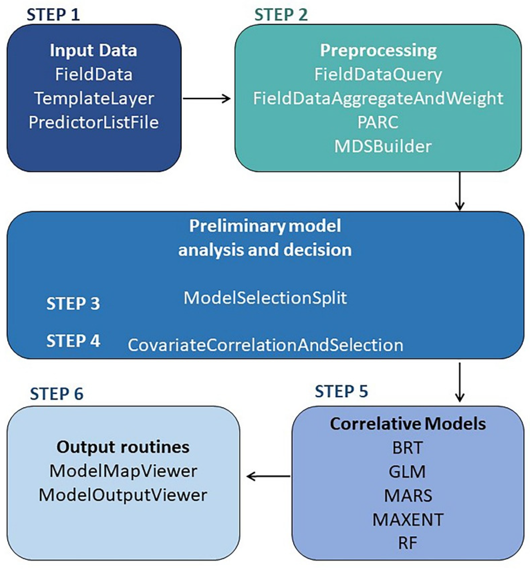
Model formulation included 6 fundamental steps (Figure 1). In the first step, predictor and citrus georeferenced data were considered. A TemplateLayer with a specific pixel size in a geographic coordinate system was defined and applied to the subsequent modelling. The second step involved synchronization of all layers by using the Projection, Aggregation, Resampling, and Clipping (PARC) module to match the template layer properties. The preliminary analysis carried out in the third step consisted of data splitting: 70% of the data was used for training and 30% for testing. In Step 4, uncorrelated predictors were selected by using the CovariateCorrelationandSelection module. Step 5 consisted of tuning the parameters for the individual algorithm. Step 6 involved analyzing accuracy measures and providing a graphical output.
At the end, a sensitivity analysis was carried out on the number of input species presence points and on the predictors’ resolution imposed by the TemplateLayer, which also affects the output.

2.1. Study Area Description

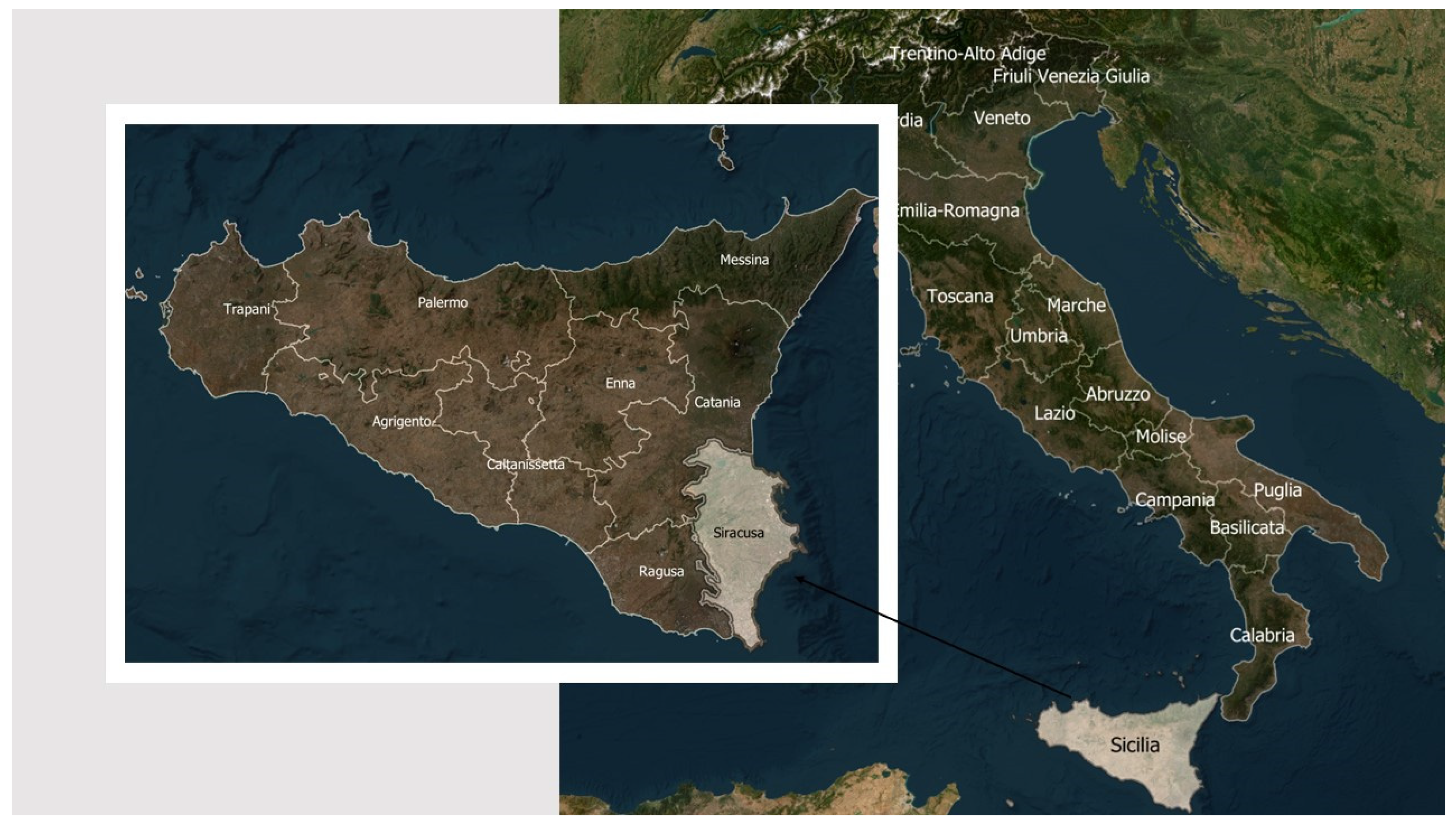
The case study was the province of Syracuse, in Sicily (Italy) (Figure 2), since this is a widely cultivated citrus growing area. Moreover, it represents one of the major citrus-producing areas in Italy. According to the 2014 ISTAT census, 17,000.00 ha are cultivated with citrus in the province with a production of about 350 million t [25]. The province of Syracuse has an area of approximately 2100 km2 and borders with the Ionian Sea to the east and with the Catania plan to the north, whereas the south of the province is characterized by the Hyblaean mountains (Figure 2).

2.2. Presence Data Gathering and Production of Predictors’ Maps

Predictors in raster format and citrus geolocation data in vector format were gathered and prepared for the first step, and the specific Templatelayer module considered in this study had a pixel size of 20 m in a WGS84 geographic coordinate system.
The simulation period was related to the year 2000 and citrus presence data were acquired for that year. The points of presence were identified by using the Sicilian Technical Regional Cartography (TRC) and IT2000 orthophotos available in the Sicilian Land Information System (SITR) (https://www.sitr.regione.sicilia.it/portal/home/item.html?id=06b441f103024aa4b1b9f966b1e4e3f9, accessed on 23 September 2022). Both maps were overlapped in GIS software (ArcGIS® for Desktop 10.3 and QGIS 3.10.0) to obtain a new map. This overlap allowed us to obtain a map with precise localization of presence points.
The resulting dataset was composed of 10,000 citrus presence points and represented as UTM WGS84 coordinates. This dataset was used as input data in VisTrails:SAHM. Pseudoabsence points cannot be included, as in Young [26], because historical data were not available. Furthermore, pseudoabsence points could be affected by anthropic activity, e.g., when citrus plants are eradicated due to reasons unrelated to crop unsuitability in that area, such as phytopathologies.
Linked to PARC, the PredictorsListFile module allowed us to add predictors in the MDSBuilder module. The considered predictors were as follows: 19 bioclimatic variables defined by WorldClim [27]; the Digital Terrain Model (DTM); soil physical properties; and irrigation.
The 19 bioclimatic variables (Table 1) for the three decades from 1970 to 2000 were acquired from the WorldClim database (https://www.worldclim.org/data/worldclim21.html, accessed on 23 September 2022) in .tiff format by using GIS tools. In most of the literature, WorldClim data are utilized for this kind of studies as they are suitable to give a broad representation of monthly, seasonal, and annual bioclimatic conditions.
In addition, the set of predictors was enriched by the DTM of the area, which provided valuable information on the height at which plant occurrence could be most probable. This layer was acquired from the Sicilian Region Land Information System website (https://www.sitr.regione.sicilia.it/portal/apps/webappviewer/index.html?id=f3f54ac44ae04a3584885eaaf0b84d70, accessed on 23 September 2022), with a resolution of 20 m, and DTM_20 was the associated predictor variable name in this study.
Soil physical properties were acquired from the European Soil Database and soil properties webpage (available at https://esdac.jrc.ec.europa.eu/resource-type/european-soil-database-soil-properties, accessed on 23 September 2022) and entered as categorial variable in SAHM software.
The irrigation variable points were acquired from the A.C.Q.U.A. project (“Agrumicultura Consapevole della Qualità e Uso dell’Acqua”—“Awareness of Quality and Use of Water in Citrus Cultivation”) [28]. These irrigation data were converted into continuous data in order to produce a raster map of the variable, named Sir_Irr (m3 ha−1) hereafter, by using the “Kriging Ordinary” interpolation method with default settings.
All layers were transformed to match the template layer properties by using the PARC module of the SAHM. The bilinear method for resampling was utilized, while the mean and majority filter methods for aggregation were selected for continuous and categorical predictors, respectively.
In fact, model implementation requires that rasters are perfectly overlapping and have exactly the same number of cells; therefore, a single raster mask delimiting the study area was defined in VisTrails:SAHM to ensure that all raster layers had the same dimensions and was carried out by coupling Templatelayer and PARC modules.
In addition, 10,000 randomly generated background points were considered in the Merged Data Set (MDS) Builder module.

2.3. Fine-Tuning Models’ Parameters

The SAHM uses 5 models with various default parameters. In this study, the values of the main parameters were modified by using data available in the literature to assess whether model performance improved.
In the following, the relevant specific settings of the five models (MaxEnt, Boosted Regression Tree, MARS, Generalized Linear Model, and Random Forest) used in VisTrails:SAHM are reported in order to define the parameters and the values considered.
The three main parameters in the BRT model are the Learning Rate (LR), the Tree Complexity (TC), and the Number of Trees (NT).
The BRT algorithm begins with a single decision tree, and then trees are added. Adding trees explains the error better with a deviance reduction. Based on this principle, increasing the number of trees reduces the impact of each tree [29]. When the default setting is applied, the BTR model adjusts the parameter values based on the input data by autoregulation [6,30]. BRT generally suffers from overfitting [31], which takes place when the fit between predicted values and actual data in models with a large number of predictors is misleadingly good [32]. Overfitting often occurs when a great number of predictors is selected in the Pearson–Spearman–Kendall matrix and may cause random errors in the results. Therefore, although more complicated models may seem more suitable, the predictions they produce may be poorer [33].
GLM is a linear regression method where a predictor is selected to be included or dropped from the considered set of predictors based on a predefined Simplification Method to minimize overfitting [34]. In this study, the influence of the Simplification Method on the GLM model by using Akaike information criterion (AIC) or Bayesian information criterion (BIC) was assessed.
MARS fits piecewise logistic regression models to presence/absence data. The MARS model overfitting is controlled by a penalty term (MarsPenalty) that can optionally be set by the user [5].
MaxEnt uses presence-only data to predict the distribution of a species based on the theory of maximum entropy [35]. In the MaxEnt model within SAHM software, one of the most important parameters is the BetaMultiplier (named Regularization Multiplier in MaxEnt software) [29]. Other MaxEnt parameters considered in this study were Replicates and Maximum Iterations.
The RF is a widely used and high-performing machine learning technique. It is an ensemble of classification or regression trees [36]. The RF model has three main parameters [37]: the number of trees (NTrees), the number of possible directions for splitting at each node of each tree (MTry), and the number of observations in each cell below which the cell is not split (NodeSize).
The value of NTrees produced by the algorithm autoregulation in this study was equal to 1000. With regard to MTry, Biau [36] demonstrated that this parameter exerts a minor impact on the model performances, and in some cases [37], high values of MTry were found to be associated with a reduction in the predictive performance. The NodeSize value can be set to 1 for classification or to 5 for regression. In this study, the influence of the choice between two values was assessed.
The default or autoregulated values and the refined values of the above-described parameters considered in this study are reported in Table 2. The refined values of the parameters were set according to the findings of some authors [22,30,38,39,40,41,42]. Table 2 also reports the parameter ranges considered in a number of simulation analyses carried out to assess how the algorithms are affected by a broader change in parameter settings. Therefore, the SAHM software was applied by using the following parameter settings (Table 2): (a) default/autoregulation values; (b) values in the range analyzed; (c) refined values based on the literature. Simulations performed with (a) settings were compared to those with (c), while simulations with (b) settings gave additional information on model sensitivity to parameter settings.

2.4. Sensitivity of the Model for Number of Presence Data and Raster Resolution

The number of presence data was reduced to find out the model sensitivity to this input, from 10,000 to 250 points.
In previous research [43], the modification of the rate between the dataset for training and testing highlighted a good robustness of the models; therefore, the percentage was set to 70% for training and 30% for testing.
Response curves were computed for the simulations at different amounts of input presence data. These response curves describe a measure of predictors’ importance in explaining the species distribution in the territory [44] by providing the general relationship between each predictor range and the suitability for the species. These curves represent a useful tool for experienced researchers to assess the outcomes of the elaborations by the biological meaning of the species.
Input raster resolution was modified from 20 m to 1 km by using the QGIS software to verify the sensitivity of the models to a change in resolution; these analyses were also carried out in relation to the number of input presence points ranging from 250 to 10,000.

2.5. Assessment of Models’ Applications

Evaluation accuracy measures derived from the confusion matrix, i.e., True Skill Statistic (TSS), and the Area Under the Receiver Operating Characteristic Curve (AUC), a standard statistical method widely used to evaluate the accuracy of species distribution models, were utilized to assess the model results and allowed comparisons between them.
The greater the Area Under the Curve (i.e., the closer the curve is to the top of the graph), the greater the discriminating power of the test. The significant AUC values are between 0.5 and 1.0 [45]. Prediction accuracy is considered to be similar to random for AUC values lower than 0.5; poor for values in the range 0.5–0.7; fair in the range 0.7–0.9; and excellent for values greater than 0.9 [46]. Moreover, ΔAUC values between training and testing greater than 0.05 indicate that the model is subjected to overfitting.
TSS values range between −1 (performance no better than random) and +1 (perfect agreement) [45].

3. Results

To facilitate comparison between maps, for each simulation, the threshold computed by SAHM for each model was acquired to convert the continuous probability maps into binary maps that identify suitable and unsuitable territorial areas for citrus. The threshold method of probability computes the threshold value by considering equal the probability that the model correctly classifies a suitable area and the probability that the model correctly classifies an unsuitable area (i.e., Sensitivity = Specificity) [24].

3.1. Fine-Tuning Models’ Parameters

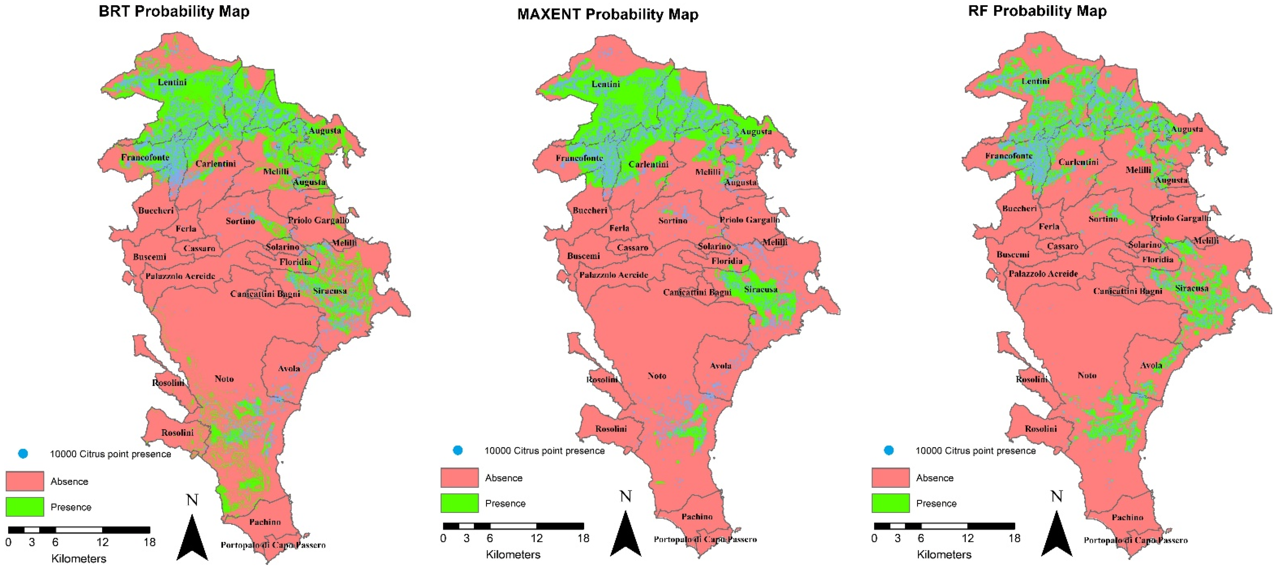
The execution of the five different algorithms was carried out by using the values of the models’ parameters described in Section 2.3. Specific sensitivity analyses were performed by modifying the default values of the parameters one at a time and keeping the others at their default values. This analysis, based on refined parameters, was compared with that performed by using default parameters and model autoregulation, obtained in a previous study [19], the main results of which are reported in Figure 3 and Table 3 (and Supplementary Materials, Figure S1) to facilitate the comparison with the outcomes of this study.
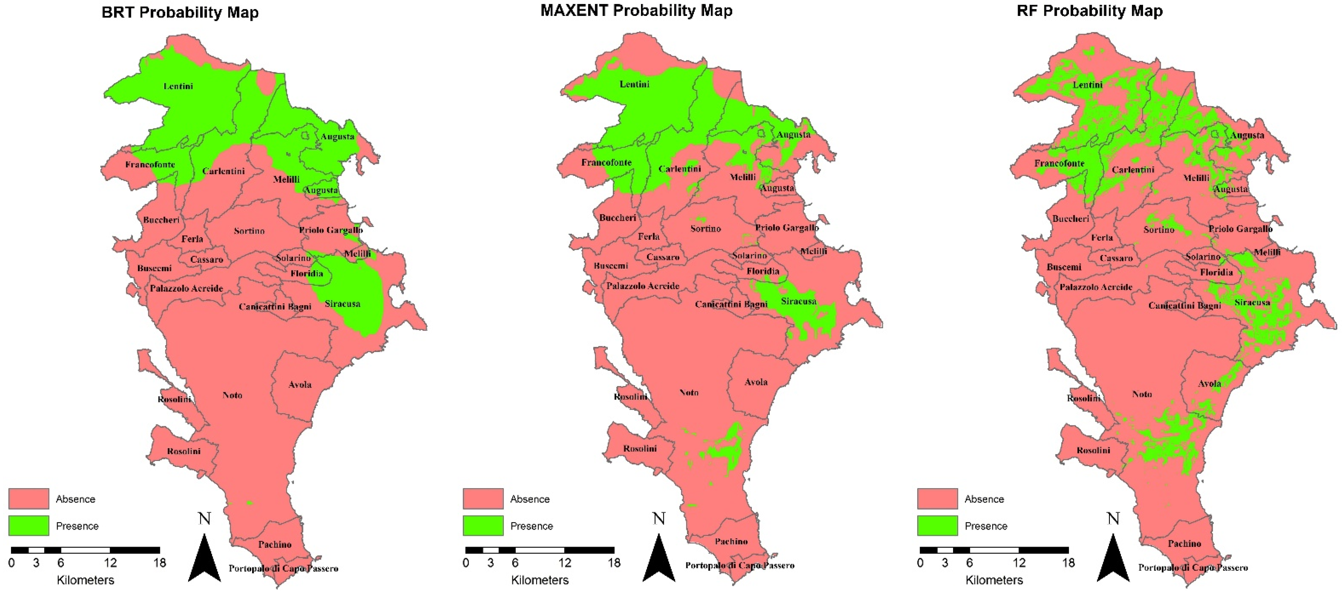
The analysis based on refined parameters produced the results reported in Figure 4 and Table 4.
The ΔAUC value for BRT improved, showing a reduction in overfitting, while the other accuracy measures decreased, though they were still above the threshold of fair prediction accuracy. However, this simulation by BRT was incoherent from the point of view of the citrus species distribution in the territory due to the absence of the species in the southern area of the province and a general increase in less detailed predicted areas for the species (i.e., more uniform areas without holes).
Moreover, from the sensitivity analyses performed, in relation to increments of LR from 0.001 to 0.1, predicted areas for the species decreased to the point of determining no presence in some areas, and corresponding ΔAUC values increased. Finally, by increasing NTrees, from 500 to 5000, the predicted surface area increased, though elaboration time increased, as also observed by Elith [29].
Sensitivity of parameters for GLM and MARS produced low variations for both predicted presence of the species and accuracy measures.
For MaxEnt, by increasing the BetaMultiplier (i.e., 0.5, 1, 1.5, 3, and 5), the AUC values progressively decreased (from 0.86 to 0.83), and ΔAUC reduced from 0.014 to 0; therefore, overfitting decreased but model performance was reduced. The choice of a high value of this parameter could be useful in the cases when MaxEnt suffers from overfitting, with the aim of keeping it one of the available models.
As regards the amplitude and distribution of predicted surfaces in the study area, the increase in the regulator value reduces the quality of the model simulation. In fact, a low regulator equal to 0.5 produced a smaller and more detailed predicted surface; when increasing the regulator, citrus presence is no longer predicted in the southern zone of the province.
For the RF model, the application of the value 5000 for NTrees, compared to the value 500, produced an increase in computational times and small differences in the results, both for the accuracy measures (AUC increased from 0.88 to 0.89) and in the distribution of the predicted surfaces. MTry and NodeSize variations did not significantly affect the results; this finding could be related to the high number of input presence points [42].
In conclusion, the comparison between Table 3 and Table 4 shows that GLM, MARS, and RF models provided more stable results, with surface area variations ranging from 0 to about 17 km2. The variations in parameter settings produced a slight impact on BRT model outcomes (surface area variation equal to 43.24 km2) and the highest on MaxEnt model findings (surface area variation equal to 223.60 km2). For this latter model, the prediction is highly modified in the south and northeast areas of the province (especially within Sortino municipality) and, thus, in the areas having a lower number of input points of citrus presence.
Table 4 shows that all models performed much better than random (AUC > 0.5) since they all exhibited AUCs > 0.8. Moreover, all models produced TSS > 50%. The models RF, MaxEnt, GLM, MARS, and BRT models showed, in that order, high predictive performance for training, whereas in terms of consistent evaluation accuracy measures between training and testing, RF, MARS, and GLM performed better than MaxEnt and BRT.
In summary, the use of the specific parameters suggested by the literature made it possible to reduce the overfitting for the BRT, but with a decrease in the AUC value, from 0.91 to 0.81, an increase in the TSS for all models was encountered.

3.2. Sensitivity of the Model for the Number of Presence Data

The modification of the input presence points determined a variation in SDM predictions and in the accuracy measures. For instance, the higher the reduction in input presence points, the higher the reduction in predicted presence for BRT, MARS, and GLM models in the eastern and southern areas where the number of input points is lower (i.e., about 13% of the input points). All the models showed an increase in the surface area of the predicted presence when increasing the number of input presence points. The GLM model predicted a wider surface in the north of the study area compared to the other models, while in MARS, the surface widened in the south. When the number of input points reduced, the RF model preserved the presence areas but with less detail (i.e., more uniform areas without holes) (see Supplementary Materials, Figure S3).
Furthermore, the analysis of the surface data highlights that for the GLM, MARS, and RF models, the predicted surface area decreases as the input points increase, making the results more refined (Table 5).
By analyzing the accuracy measures, the models GLM and RF were found to be influenced by the reduction in the number of input points, whereas the MARS, BRT, and MaxEnt models were less affected.
With regard to AUC, the BRT model showed high AUC (i.e., a range between 0.91 and 0.94 for the training). However, there was overfitting for all the hypotheses since ΔAUC values were higher than 0.05. Conversely, the other models were less affected by overfitting with a maximum value of ΔAUC equal to 0.04, produced by MaxEnt for the 250-point simulation. The GLM model showed AUC values between 0.81 and 0.82, and reached a value of 0.85 in the simulation at 10,000 points. The MARS (AUC = 0.82–0.83) and MaxEnt (AUC = 0.86–0.88) models did not exhibit large variations. The RF model (AUC = 0.83–0.88) was initially affected by the lower number of points and reached the maximum AUC value in the simulation at 10,000 points.
With regard to the analysis of the TSS values, the RF model produced a gradual increase in the values as the number of input points increased, from 0.49 for 250 points to 0.62 for 10,000 points, and a minimum of 500 input points was required to have TSS ≥ 0.5. GLM and MARS were stable on values around the threshold of 0.5 and exceeded it only in the simulation at 10,000 points; therefore, for these models, it is advisable to have a large number of input presence data. TSS generally decreased as input points increased, with minimum values of 0.55 and 0.65 (for training) in the 10,000-point simulation, for MaxEnt and BRT, respectively.
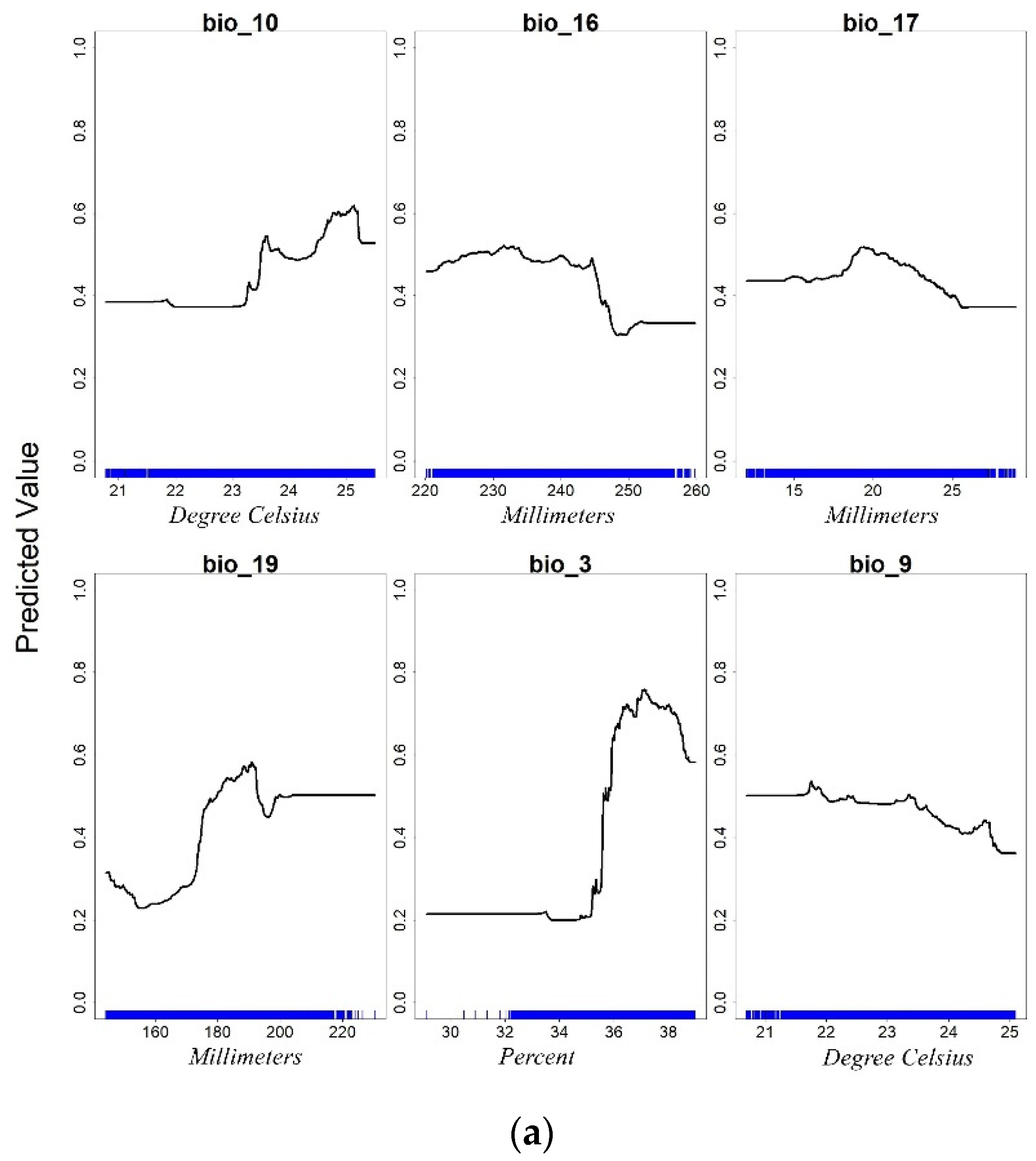
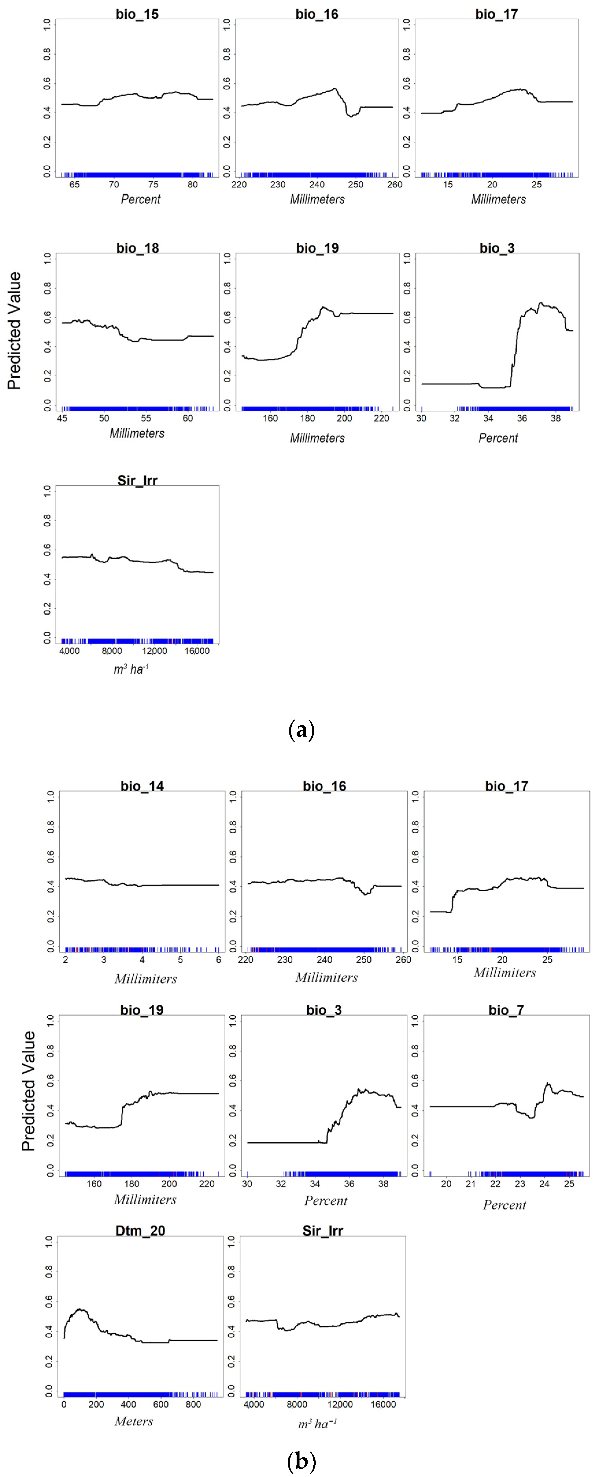
With regard to response curves, the simulations of RT model for 250 and 10,000 input points are reported in Figure 5. This figure graphically depicts the shape and the magnitude of the covariates, displaying the link between the values of the covariates and the citrus suitability according to the predictions of the RF algorithm.
When the input points were reduced from 10,000 to 250, the number of predictors decreased from 8 (i.e., BIO_15, BIO_16, BIO_17, BIO_19, BIO_3, BIO_9, DTM_20, Sir_Irr) to 6 (i.e., BIO_10, BIO_16, BIO_17, BIO_19, BIO_3, BIO_9). The biovariables had a major effect in explaining the citrus presence with 250 input points, whereas biovariables had a lower effect with 10,000 input points since DTM_20 and Sir_Irr became influencing parameters. Consequently, at the 250-input-point simulation, the contribution of biovariables to the predicted value was higher, markedly in some cases, such as those of Bio_3 (Isothermality) and Bio_9 (Mean Temperature of Driest Quarter).
Isothermality (BIO_3) showed a left-skewed response curve and a maximum suitability between 35% and 38%; this range would indicate that high suitability is connected to lower variability of daily and nightly temperatures within a month compared to the year.
The shape of the curves generally changed, especially for Bio_16 (Precipitation of Wettest Quarter), which reduced its contribution for values above 245 mm, and for the maximum contribution of Bio_17 (Precipitation of Driest Quarter), which shifted from 24 to 20 mm on the x axis. Elevation (Dtm_20) contributed up to about 400 m, as previously found [19], and irrigation (Sir_irr) provided a constant contribution in its range of variation.
Bio_15 (Precipitation Seasonality) exhibited a constant curve with the highest values ranging between 68% and 80%. This predictor describes the variability of the precipitations in the year; the higher the index value, the higher the variability of the precipitations. According to the Intergovernmental Panel on Climate Change 2012 report, high variability indicates a concentration of precipitation in a short period of time, such as in Mediterranean regions [47].
Bio_19 (Precipitation of Coldest Quarter) exhibited a sigmoid response curve with the highest values above 180 mm.

3.3. Sensitivity of the Model to Resolution

A comparison between 20 m resolution and 1 km resolution simulations, keeping the number of input presence points equal to 10,000, and reducing it to 250, allowed us to analyze whether the models were affected by resolution and to what extent when input presence data were modified.
In Figure 6 (and Supplementary Materials, Figure S4), the maps of the 1 Km simulations carried out by the different models are reported for the 10,000-point simulation. In green color, the areas of predicted presence generally encompass the input presence points (in blue), except for GLM, which failed most to simulate correctly in the southeastern coastal area of the province (mainly in Avola and Noto municipalities) and also in the central one (Sortino municipality). The comparison of these maps (Figure 6 and Figure S4) with those at a 20 m resolution (Figure 3) confirm the failure of GLM, and of MARS to some extent, to predict the citrus presence in those areas and in the south of the province. Overall, the lower the resolution, the higher the surface areas of predicted presence (Table 6); in detail, the difference between the values of surface areas for the two resolutions (S20m − S1km) ranged between 182.2 km2 of BRT and 411.7 km2 of RF, except for MaxEnt, which decreased by 47.1 km2.
The reduction in spatial resolution to 1 km produced a general reduction in the models’ performance in terms of accuracy measures (Table 7) compared to values associated with 20 m resolution (Table 3). The values of TSS indicated a low accuracy for the models, and the AUC values dropped drastically by about 0.2. Conversely, overfitting was not encountered in the 10,000-point simulations, as the values related to ΔAUC10,000 of the models did not reach the threshold of 0.05. At 250 input presence points, the values of AUC were high (>0.75) but with a high overfitting for BRT and RF, whereas the TSS decreased under 0.5 for GLM, MARS, and RF.
At a resolution of 1 km (Figure 7), the increase in the input points produced an increase in the covariate number, and the general remarks described for the 20 m resolution simulation (Section 3.2) were confirmed. Thus, the contribution of the 19 biovariables to the predicted value decreased when increasing the number of input points, and the influence of DTM_20 and Sir_Irr increased. Thermal and precipitation biovariable ranges adequately described the climatic conditions in Mediterranean regions; in fact, Bio_7 (Temperature Annual Range) predictor, ranging between approximately 20 °C and 25 °C, was in the interval considered for citrus species in Spain [48], and the values of the variability of the precipitations (Bio_15) as well as the precipitation in the driest quarter (Bio_17) effectively denoted the precipitation scarcity in the territory.
4. Discussion

The analyses carried out in this study on models’ parameters allowed for the investigation of the performance of the models in relation to a specific case study.
Based on refined parameters, the analysis of the maps produced by the SDMs showed significant changes in the prediction of the BRT model. In detail, a reduction in overfitting was obtained compared to default parameters. The prediction showed more uniform areas and a lower precision in the southern area compared to the prediction with default parameters.
In this regard, in a previous study by Catalano et al. [19], the BRT model was found to suffer from overfitting compared to other models. Since, according to Elith [30], the specific features of BRT raise a number of practical issues in model fitting, in this study, the model outcomes were assessed from a territorial point of view. The results of this research study optimized the use of the BRT with benefits in terms of the accuracy and applicability of the model.
Similarly, the MaxEnt model was affected by the changes in the parameters’ settings in the eastern and southern areas, where there were a lower number of input presence points. In a study by West et al. [22], the authors suggested considering different factors (i.e., Slope, Eastness, Greenness index, Solar radiation) to predict invasive species distribution; therefore, further simulation efforts could be made in future studies to broaden the number of predictors for a more precise identification of the drivers of species occurrence. Based on the literature, the MaxEnt model can be considered a promising tool for land managers to carry out an initial assessment of species suitability for a territory, since it is possible to obtain a prediction with a small initial set of data points, when time and resources are limited.
GLM, MARS, RF, and MaxEnt were the best performing models, while BRT underperformed regardless of the changed parameters. In fact, the self-tuning capability of the BRT can be reduced by the settings of the model parameters [6]. Differences in model performance are often associated with model complexity; models with longer running times appear to produce better accuracy measures [2].
With regard to RF, as confirmed by Diaz [42], the MTry parameter can lead to higher error rates when few input presence points are used. This confirms the importance of working on large amounts of input data and that, in this case study, no significant effects were observed due to the 10,000 input presence points. In fact, models trained with a large number of occurrences generally outperform models built with a lower number of occurrences, and also have less variation in their results. These findings suggest that models trained with an insufficient number of species occurrences are less likely to perform well. Therefore, the use of a high number of background points (i.e., 10,000 in this case study) and a suitable number of presence points related to the investigated surface increased the performance and prediction of SDMs. This is in line with the study of Barbet-Massin [49].
In this study, the number of input presence data was found to affect the MARS, BRT, and MaxEnt models less in terms of accuracy. Therefore, these models could be more suitably applied in simulations where multiple species are considered and a different amount of input presence data is available for the various species. However, overfitting is a key weakness to be duly considered in the choice of the model to apply; BRT, for instance, exhibited this drawback for its application in this study, as observed in other studies [31].
In this study, elevation was among the main predictors, when a high number of presence points were considered. In detail, it indicated the suitability of the species up to a value of 400 m. Therefore, in the specific territory, it would suggest that the species distribution is driven by a temperature reduction due to an increase in elevation, following the gradient south–north. Therefore, areas located above 400 m presented marginal climatic conditions for citrus cultivation.
However, model performance was found to be greatly affected by the resolution. The spatial scale of the study was affected by the study extent and the resolutions of the available input rasters (i.e., the resolution ranged from a 20 m DTM, and a high presence data density, to the 1 km resolution of WorldClim biovariables). This prompted us to consider that DTM could have a higher effect on the probability of presence compared to bioclimatic variables that were less detailed.
According to Phillips et al. [42], MaxEnt is a robust method well suited to species distribution modelling for biodiversity conservation and climate change prediction. The MaxEnt model is one of the most applied models and the impact of beta-regulations on performance and final results has been investigated. Based on the results obtained, the regulator penalized the areas with fewer input presence points. Therefore, whether the regulator value is related to the number of input presence points should be investigated.
According to Guisan [16], it is necessary to carry out more tests to determine the resolution ratio, the number of points, and the extension of the study area for a good prediction result since the significant influence of the grain size could be due to multiple factors. For example, the use of a low resolution encloses different conditions in one pixel and consequently would lead to the selection of unsuitable habitats for the plant.
Conversely, the use of a high resolution can lead to forced resampling and, consequently, the result could not provide consistent information under real conditions.

5. Conclusions

Fitting an SDM involves a series of steps that requires different choices and well-justified decisions. This study has investigated the effect of changing algorithms parameters and data width on SDM performance.
The results demonstrated that the number of presence points has a key impact on the expected presence of the species. It is crucial to consider an adequate number of input presence points in relation to the SDM sensitivity to this parameter, bearing in mind that all the outcomes should be assessed from an agricultural point of view. Furthermore, the resolution chosen for the input levels must be proportional to the study area and the number of input presence points to maximize model performance and obtain reliable predictions. The reliability of the prediction is related both to the parameters’ optimization as well as its representativeness in a real context. In fact, a reliable prevision should check whether the output of the models is in line with the crop distribution, soil features, and environmental conditions.
Although this modelling application included models’ parameters and many variables with effects on covariates and presence data width, further research is needed to explore other potential important predictors and their quality. In fact, in the context of crop suitability mapping, uncertainties may arise by a number of other circumstances such as the adoption of novel techniques, new crop varieties, specific economic drivers, and trade that could influence crop production. Thus, the effort to introduce new spatial explicit predictors’ data related to those drivers of change in the species distribution could significantly improve the connected models’ predictive capability for sustainable resource management and land planning.
The outcomes of this study have broadened the information basis, thus contributing to support utilization of SDMs, coupled with GIS tools, in studies related to the environmental sector and sustainable use of resources.

Supplementary Materials

The following supporting information can be downloaded at: https://www.mdpi.com/article/10.3390/su15097656/s1, Figure S1: Probability maps of species distribution for a 0.8 value for Pearson-Spearman-Kendall coefficients threshold, 10,000 presence points, default values of models’ parameters, and 20-m resolution, for GLM and MARS models; Figure S2: Probability maps of species, with 10,000 presence points, 20-m resolution, and refined values of models’ parameters for GLM and MARS models; Figure S3: Probability maps of species distribution for 250–500–1000 presence points and for default values of parameters; Figure S4: Maps of predicted citrus presence (green) or absence (red) for the different models, at a 1-Km resolution and 1000 and 250 input presence points for GLM and MARS model.

Author Contributions

Conceptualization, C.A. and G.A.C.; methodology, C.A. and G.A.C.; software, G.A.C.; validation, P.R.D. and C.A.; formal analysis, P.R.D. and F.M.; investigation, P.R.D. and C.A.; resources, C.A.; data curation, G.A.C. and F.M.; writing—original draft preparation, C.A. and G.A.C.; writing—review and editing, C.A., F.M. and P.R.D.; visualization, P.R.D.; supervision, C.A.; project administration, C.A.; funding acquisition, C.A. All authors have read and agreed to the published version of the manuscript.

Funding

The research study was funded and APC entirely paid by the University of Catania through the project ‘PON “RICERCA E INNOVAZIONE” 2014–2020, Azione II—Obiettivo Specifico 1b—Progetto “Miglioramento delle produzioni agroalimentari mediterranee in condizioni di carenza di risorse idriche—WATER4AGRIFOOD”, Cod. progetto: ARS01_00825, CUP: B64I20000160005. This study was also carried out in line with the Agritech National Research Center and received funding from the European Union Next-GenerationEU (PIANO NAZIONALE DI RIPRESA E RESILIENZA (PNRR)—MISSIONE 4 COMPONENTE 2, INVESTIMENTO 1.4—D.D. 1032 17/06/2022, CN00000022). This manuscript reflects only the authors’ views and opinions, neither the European Union nor the European Commission can be considered responsible for them.

Institutional Review Board Statement

Not applicable.

Informed Consent Statement

Not applicable.

Data Availability Statement

Data are available on request.

Acknowledgments

The authors wish to thank the Sicilian Region for SITR data (https://www.sitr.regione.sicilia.it/, accessed on 23 September 2022).

Conflicts of Interest

The authors declare no conflict of interest.

References

  1. Cramer, W.; Guiot, J.; Fader, M.; Garrabou, J.; Gattuso, J.P.; Iglesias, A.; Lange, M.A.; Lionello, P.; Llasat, M.C.; Paz, S.; et al. Climate change and interconnected risks to sustainable development in the Mediterranean. Nat. Clim. Chang. 2018, 8, 972–980. [Google Scholar] [CrossRef]
  2. Akpoti, K.; Kabo-Bah, A.T.; Dossou-Yovo, E.R.; Groen, T.A.; Zwart, S.J. Mapping suitability for rice production in inland valley landscapes in Benin and Togo using environmental niche modeling. Sci. Total Environ. 2020, 709, 136165. [Google Scholar] [CrossRef]
  3. Elith, J.; Leathwick, J.R. Species distribution models: Ecological explanation and prediction across space and time. Annu. Rev. Ecol. Evol. Syst. 2019, 40, 677–697. [Google Scholar] [CrossRef]
  4. Baer, K.C.; Gray, A.N. Biotic predictors improve species distribution models for invasive plants in Western US Forests at high but not low spatial resolutions. For. Ecol. Manag. 2022, 518, 120249. [Google Scholar] [CrossRef]
  5. West, A.M.; Jarnevich, C.S.; Young, N.E.; Fuller, P.L. Evaluating potential distribution of high-risk aquatic invasive species in the water garden and aquarium trade at a global scale based on current established populations. Risk Anal. 2019, 39, 1169–1191. [Google Scholar] [CrossRef]
  6. Yang, X.Q.; Kushwaha, S.P.S.; Saran, S.; Xu, J.; Roy, P.S. Maxent modeling for predicting the potential distribution of medicinal plant, Justicia adhatoda L. in Lesser Himalayan foothills. Ecol. Eng. 2013, 51, 83–87. [Google Scholar] [CrossRef]
  7. Yi, Y.J.; Cheng, X.; Yang, Z.F.; Zhang, S.H. Maxent modeling for predicting the potential distribution of endangered medicinal plant (H. riparia Lour) in Yunnan, China. Ecol. Eng. 2016, 92, 260–269. [Google Scholar] [CrossRef]
  8. Nascimbene, J.; Casazza, G.; Benesperi, R.; Catalano, I.; Cataldo, D.; Grillo, M.; Isocrono, D.; Matteucci, E.; Ongaro, S.; Potenza, G.; et al. Climate change fosters the decline of epiphytic Lobaria species in Italy. Biol. Conserv. 2016, 201, 377–384. [Google Scholar] [CrossRef]
  9. Brun, P.; Vogt, M.; Payne, M.R.; Gruber, N.; O’Brien, C.J.; Buitenhuis, E.T.; Le Quéré, C.; Leblanc, K.; Luo, Y.-W. Ecological niches of open ocean phytoplankton taxa. Limnol. Oceanogr. 2015, 60, 1020–1038. [Google Scholar] [CrossRef]
  10. Diniz-Filho, J.A.F.; Mauricio Bini, L.; Fernando Rangel, T.; Loyola, R.D.; Hof, C.; Nogués-Bravo, D.; Araújo, M.B. Partitioning and mapping uncertainties in ensembles of forecasts of species turnover under climate change. Ecography 2009, 32, 897–906. [Google Scholar] [CrossRef]
  11. Zouabi, O.; Kadria, M. The direct and indirect effect of climate change on citrus production in Tunisia: A macro and micro spatial analysis. Clim. Chang. 2016, 139, 307–324. [Google Scholar] [CrossRef]
  12. Ashraf, U.; Ali, H.; Chaudry, M.N.; Ashraf, I.; Batool, A.; Saqib, Z. Predicting the Potential Distribution of Olea fer-ruginea in Pakistan incorporating Climate Change by Using Maxent Model. Sustainability 2016, 8, 722. [Google Scholar] [CrossRef]
  13. Leanza, P.M.; Valenti, F.; D’Urso, P.R.; Arcidiacono, C. A combined MaxEnt and GIS-based methodology to estimate cactus pear biomass distribution: Application to an area of southern Italy. Biofuels Bioprod. Biorefin. 2022, 16, 54–67. [Google Scholar] [CrossRef]
  14. Qiao, L.; Mayer, C.; Liu, S. Distribution and interannual variability of supraglacial lakes on debris-covered glaciers in the Khan Tengri-Tumor Mountains, Central Asia. Environ. Res. Lett. 2015, 10, 014014. [Google Scholar] [CrossRef]
  15. Jarnevich, C.S.; Stohlgren, T.J.; Kumar, S.; Morisette, J.T.; Holcombe, T.R. Caveats for correlative species distribution modeling. Ecol. Inform. 2015, 29, 6–15. [Google Scholar] [CrossRef]
  16. Guisan, A.; Graham, C.H.; Elith, J.; Huettmann, F.; the NCEAS Species Distribution Modelling Group. Sensitivity of predictive species distribution models to change in grain size. Divers. Distrib. 2007, 13, 332–340. [Google Scholar] [CrossRef]
  17. Istat. Atlante dell’agricoltura in Sicilia. In Una Lettura Guidata Delle Mappe Tematiche; Istat: Rome, Italy, 2014. [Google Scholar]
  18. Del Bravo, F.; Finizia, A.; Lo Moriello, M.S.; Ronga, M. La competitività della filiera agrumicola in Italia. Rete Rural. Naz. 2014, 2020, 2020. [Google Scholar]
  19. Catalano, G.A.; Maci, F.; D’Urso, P.R.; Arcidiacono, C. GIS and SDM-Based Methodology for Resource Optimisation: Feasibility Study for Citrus in Mediterranean Area. Agronomy 2023, 13, 549. [Google Scholar] [CrossRef]
  20. Miller, J. Species Distribution Modeling. Geogr. Compass 2010, 4, 490–509. [Google Scholar] [CrossRef]
  21. Jarnevich, C.S.; Talbert, M.; Morisette, J.; Aldridge, C.; Brown, C.S.; Kumar, S.; Manier, D.; Talbert, C.; Holcombe, T. Minimizing effects of methodological decisions on interpretation and prediction in species distribution studies: An example with background selection. Ecol. Model. 2017, 363, 48–56. [Google Scholar] [CrossRef]
  22. West, A.M.; Kumar, S.; Brown, C.S.; Stohlgren, T.J.; Bromberg, J. Field validation of an invasive species Maxent model. Ecol. Inform. 2016, 36, 126–134. [Google Scholar] [CrossRef]
  23. Hayes, M.A.; Cryan, P.M.; Wunder, M.B. Seasonally-dynamic presence-only species distribution models for a cryptic migratory bat impacted by wind energy development. PLoS ONE 2015, 10, e0132599. [Google Scholar] [CrossRef] [PubMed]
  24. Chang, T.; Hansen, A.J.; Piekielek, N. Patterns and variability of projected bioclimatic habitat for Pinus albicaulis in the Greater Yellowstone Area. PLoS ONE 2014, 9, e111669. [Google Scholar] [CrossRef] [PubMed]
  25. Valenti, F.; Porto, S.M.; Chinnici, G.; Cascone, G.; Arcidiacono, C. A GIS-based model to estimate citrus pulp availability for biogas production: An application to a region of the Mediterranean Basin. Biofuels Bioprod. Biorefin. 2016, 10, 710–727. [Google Scholar] [CrossRef]
  26. Young, N.E.; Jarnevich, C.S.; Sofaer, H.R.; Pearse, I.; Sullivan, J.; Engelstad, P.; Stohlgren, T.J. A modeling workflow that balances automation and human intervention to inform invasive plant management decisions at multiple spatial scales. PLoS ONE 2020, 15, e0229253. [Google Scholar] [CrossRef] [PubMed]
  27. O’donnell, M.S.; Ignizio, D.A. Bioclimatic predictors for supporting ecological applications in the conterminous United States. US Geol. Surv. Data Ser. 2012, 691, 4–9. [Google Scholar]
  28. University of Catania 2012, CREA, Distretto Agrumi Sicilia and CocaCola Foundation, A.C.Q.U.A. PROJECT RESULTS. 2020. Available online: https://www.distrettoagrumidisicilia.it/wp-content/uploads/Dossier-Acqua5.pdf (accessed on 9 June 2022).
  29. Morales, N.S.; Fernández, I.C.; Baca-González, V. Configurazione dei parametri di MaxEnt e piccoli campioni: Stiamo prestando attenzione alle raccomandazioni? Una revisione sistematica. PeerJ 2017, 5, e3093. [Google Scholar] [CrossRef] [PubMed]
  30. Elith, J.; Leathwick, J.R.; Hastie, T. A working guide to boosted regression trees. J. Anim. Ecol. 2008, 77, 802–813. [Google Scholar] [CrossRef] [PubMed]
  31. Suleiman, A.; Tight, M.R.; Quinn, A.D. Hybrid Neural Networks and Boosted Regression Tree Models for Predicting Roadside Particulate Matter. Environ. Model Assess. 2016, 21, 731–750. [Google Scholar] [CrossRef]
  32. Breiner, F.T.; Guisan, A.; Bergamini, A.; Nobis, M.P. Overcoming limitations of modelling rare species by using ensembles of small models. Methods Ecol. Evol. 2015, 6, 1210–1218. [Google Scholar] [CrossRef]
  33. Heikkinen, R.K.; Luoto, M.; Araújo, M.B.; Virkkala, R.; Thuiller, W.; Sykes, M.T. Methods and uncertainties in bioclimatic envelope modelling under climate change. Prog. Phys. Geogr. 2006, 30, 751–777. [Google Scholar] [CrossRef]
  34. Morisette, J.T.; Jarnevich, C.S.; Holcombe, T.R.; Talbert, C.B.; Ignizio, D.; Talbert, M.K.; Silva, C.; Koop, D.; Swanson, A.; Young, N.E. VisTrails SAHM: Visualization and workflow management for species habitat modeling. Ecography 2013, 36, 129–135. [Google Scholar] [CrossRef]
  35. Khanum, R.; Mumtaz, A.S.; Kumar, S. Predicting impacts of climate change on medicinal asclepiads of Pakistan using Maxent modelling. Acta Oecol 2013, 49, 23–31. [Google Scholar] [CrossRef]
  36. Biau, G.; Scornet, E. A random forest guided tour. Test 2016, 25, 197–227. [Google Scholar] [CrossRef]
  37. Valavi, R.; Elith, J.; Lahoz-Monfort, J.J.; Guillera-Arroita, G. Modelling species presence-only data with random forests. Ecography 2021, 44, 1731–1742. [Google Scholar] [CrossRef]
  38. Eilers, P.H.C.; Marx, B.D. Generalized linear additive smooth structures. J. Comput. Graph. Stat. 2002, 11, 758–783. [Google Scholar] [CrossRef]
  39. Chen, X.; Aravkin, A.Y.; Martin, R.D. Generalized Linear Model for Gamma Distributed Variables via Elastic Net Regularization. arXiv 2018, arXiv:1804.07780. [Google Scholar]
  40. Phillips, S.J.; Dudík, M. Modeling of species distributions with Maxent: New extensions and a comprehensive evaluation. Ecography 2008, 31, 161–175. [Google Scholar] [CrossRef]
  41. Phillips, S.J.; Anderson, R.P.; Schapire, R.E. Maximum entropy modeling of species geographic distributions. Ecol. Model. 2006, 190, 231–259. [Google Scholar] [CrossRef]
  42. Díaz-Uriarte, R.; Alvarez de Andrés, S. Gene selection and classification of microarray data using random forest. BMC Bioinform. 2006, 7, 3. [Google Scholar] [CrossRef]
  43. Catalano, G.A.; Maci, F.; Valenti, F.; D’Urso, P.R.; Arcidiacono, C. Application of geospatial models for suitability and distribution potential of citrus: A case study in eastern Sicily. In Proceedings of the 12th International AIIA Conference, Biosystems Engineering towards the Green Deal, Palermo, Italy, 19–22 September 2022. [Google Scholar]
  44. Naimi, B.; Araújo, M.B. Sdm: A reproducible and extensible R platform for species distribution modelling. Ecography 2016, 39, 368–375. [Google Scholar] [CrossRef]
  45. D’Arrigo, G.; Provenzano, F.; Torino, C.; Zoccali, C.; Tripepi, G. I test diagnostici e l’analisi della curva ROC. G. Ital. Nefrol. 2011, 28, 642–647. [Google Scholar] [PubMed]
  46. Di Napoli, M.; Carotenuto, F.; Cevasco, A.; Confuorto, P.; Di Martire, D.; Firpo, M.; Pepe, G.; Raso, E. Machine learning ensemble modelling as a tool to improve landslide susceptibility mapping reliability. Landslides 2020, 17, 1897–1914. [Google Scholar] [CrossRef]
  47. Saidi, H.; Dresti, C.; Ciampittiello, M. Il cambiamento climatico e le piogge: Analisi dell’evoluzione delle piogge stagionali e degli eventi estremi negli ultimi 50 anni nella stazione di Pallanza. Biol. Ambient. 2014, 28, 2. [Google Scholar]
  48. Primo-Capella, A.; Martínez-Cuenca, M.-R.; Forner-Giner, M.Á. Cold Stress in Citrus: A Molecular, Physiological and Biochemical Perspective. Horticulturae 2021, 7, 340. [Google Scholar] [CrossRef]
  49. Barbet-Massin, M.; Jiguet, F.; Albert, C.H.; Thuiller, W. Selecting pseudo-absences for species distribution models: How, where and how many? Methods Ecol. Evol. 2012, 3, 327–338. [Google Scholar] [CrossRef]
Figure 1. Pipeline of the model in VisTrails:SAHM.
Sustainability 15 07656 g001
Figure 2. Study area localization within Italy and Sicily.
Sustainability 15 07656 g002
Figure 3. Probability maps of species distribution for 10,000 presence points, default values of models’ parameters, and 20 m resolution, for BRT, MaxEnt, and RF models (maps related to GLM and MARS results are reported in Supplementary Materials, Figure S1).
Sustainability 15 07656 g003
Figure 4. Probability maps of species, with 10,000 presence points, 20 m resolution, and refined values of models’ parameters for BRT, MaxEnt, and RF models (maps related to GLM and MARS results are reported in Supplementary Materials, Figure S2).
Sustainability 15 07656 g004
Figure 5. Response Curves for RF model at 250 pt (a) and 10,000 pt (b) of input presence points, at a resolution of 20 m.
Sustainability 15 07656 g005aSustainability 15 07656 g005b
Figure 6. Maps of predicted citrus presence (green) or absence (red) for the different models, at a 1 km resolution and 10,000 (ac) input presence points (blue) and 1 km resolution and 250 input presence points (df) for BRT, MaxEnt, and RF models (maps related to GLM and MARS results are reported in Supplementary Materials).
Sustainability 15 07656 g006
Figure 7. Response curves for RF model for 250 input citrus presence points (a) and 10,000 input citrus presence points (b), at a 1 km resolution.
Sustainability 15 07656 g007
Table 1. List of the 19 bioclimatic variables.
VariablesDescriptionUnit of Measure
BIO1Annual Mean Temperature°C
BIO2Mean Diurnal Range°C
BIO3Isothermality%
BIO4Temperature Seasonality°C
BIO5Max Temperature of Warmest Month°C
BIO6Min Temperature of Coldest Month°C
BIO7Temperature Annual Range°C
BIO8Mean Temperature of Wettest Quarter°C
BIO9Mean Temperature of Driest Quarter°C
BIO10Mean Temperature of Warmest Quarter°C
BIO11Mean Temperature of Coldest Quarter°C
BIO12Annual Precipitationmm
BIO13Precipitation of Wettest Monthmm
BIO14Precipitation of Driest Monthmm
BIO15Precipitation Seasonality (Coefficient of Variation)%
BIO16Precipitation of Wettest Quartermm
BIO17Precipitation of Driest Quartermm
BIO18Precipitation of Warmest Quartermm
BIO19Precipitation of Coldest Quartermm
Table 2. Parameter settings of the models in the various simulations.
ModelsParametersDefault or Autoregulation Value [19]Parameter Range AnalyzedRefined Values
BRTLearning Rate0.0760.001–0.10.001
Tree Complexity201–53
Number of Trees300500–50001000
RFMTry11–22
NTrees1000500–5000500
NodeSize21–51
MARSMarsPenalty22–2.52.5
GLMSimplificationMethodAICAIC-BICAIC
MaxEntReplicates15–2015
Maximum Iterations50005000–10,0005000
BetaMultiplier10.5–51
Table 3. Presence and absence surface areas for species distribution and AUC values for training, 10,000 presence points, default values of parameters, and 20 m resolution.
Surface Area (km2)BRTGLMMARSMaxEntRF
Red (absence)1589.391618.611597.801426.661701.51
Green (presence)519.59484.35505.17676.30401.45
AUC for training0.910.850.830.860.88
ΔAUC0.0820.0020.0010.0060.000
Table 4. Surface areas of citrus probability of presence or absence for each SDM, and accuracy measures for training and related ΔAUC, obtained by using refined models’ parameters.
Surface Area (km2)BRTGLMMARSMaxEntRF
Red (absence)1546.141618.611597.801650.261718.07
Green (presence)562.83484.35505.16452.709384.89
AUC0.810.840.830.850.89
TSS0.740.520.510.550.62
ΔAUC0.0060.0020.0010.0060.000
Table 5. Predicted citrus surface area (km2) at different values of input presence points, for 20 m resolution, and default parameters with autoregulation.
Input Presence Points
Models 250500100010,000
BRTAbsence1778.61749.41782.81589.4
Presence330.4359.6326.1519.6
GLMAbsence1565.21577.61562.41618.6
Presence543.8531.4546.6484.4
MARSAbsence1591.41587.91579.11597.8
Presence517.6521.1529.9505.2
MaxEntAbsence1679.11665.01652.81426.7
Presence429.9444.0456.2676.3
RFAbsence1583.01648.21685.11701.5
Presence525.9460.8423.8401.5
Table 6. Surface area (km2) of predicted citrus presence or absence for the different models, at a 1 km resolution and 10,000 or 250 input presence points.
Surface Areas (km2)
Input PointsBRTGLMMARSMaxEntRF
Absence (red)10,00014821357143614531302
25016331509155616411515
Presence (green)10,000627752673656807
250476600553468594
Table 7. Accuracy measures for the different models, at a 1 km resolution and 10,000 or 250 input presence points.
BRTGLMMARSMaxEntRF
TrainingTestingTrainingTestingTrainingTestingTrainingTestingTrainingTesting
AUC2500.950.830.790.830.800.840.850.840.750.81
AUC10,0000.770.720.700.720.730.750.750.750.530.57
TSS2500.550.530.440.550.450.550.540.570.390.82
TSS10,0000.390.330.290.290.330.380.360.350.050.12
Disclaimer/Publisher’s Note: The statements, opinions and data contained in all publications are solely those of the individual author(s) and contributor(s) and not of MDPI and/or the editor(s). MDPI and/or the editor(s) disclaim responsibility for any injury to people or property resulting from any ideas, methods, instructions or products referred to in the content.