Managing Disruptions in a Biomass Supply Chain: A Decision Support System Based on Simulation/Optimisation

Abstract

To design and deploy their supply chains, companies must naturally take quite different decisions, some being strategic or tactical, and others of an operational nature. This work resulted in a decision support system for optimising a biomass supply chain in Portugal, allowing a more efficient operations management, and enhancing the design process. Uncertainty and variability in the biomass supply chain is a critical issue that needs to be considered in the production planning of bioenergy plants. A simulation/optimisation framework was developed to support decision-making, by combining plans generated by a resource allocation optimisation model with the simulation of disruptive wildfire scenarios in the forest biomass supply chain. Different scenarios have been generated to address uncertainty and variability in the quantity and quality of raw materials in the different supply nodes. Computational results show that this simulation/optimisation approach can have a significant impact in the operations efficiency, particularly when disruptions occur closer to the end of the planning horizon. The approach seems to be easily scalable and easy to extend to other sectors.

1. Introduction

The performance of a biomass supply chain (SC) heavily depends on its design and on how operations are planned, as higher levels of coordination and optimisation are required to maximise efficiency [1,2]. With sustainable and clean energy production capabilities, biomass energy can play, in the near future, a crucial role as a promising alternative to fossil fuels. Given abundant raw materials, ease of storage, and the potential for global production, the biomass industry is experiencing a significant growth, but there is still room for improvement in terms of profitability [3,4].

Efficient supply chain management is vital to reduce costs, to adapt to unexpected events, and to ensure demand fulfilment. Transportation and transformation of the wood into smaller particles (“chipping”) encompass a significant portion of the biomass supply chain costs [5]. Identifying operational sites, capacities and routes, as well as performing the right assignment of operations, is crucial to reduce forest biomass logistic costs and to face disruptive events, thus rendering supply chains more resilient [6]. In addition to its moisture content and low bulk density, the unique characteristics of forest biomass, such as availability and susceptibility to weather variability, make the design and management of these supply chains more complex and challenging [7,8].

Biomass is a renewable energy source derived from various organic materials, such as agricultural residues from trimming and harvestings, garden residues, and forest remains resulting from the timber industry, silvicultural operations, and wildfires [9,10]. All these forest residues can be harvested in multiple forms as logs, slabs of wood or already in “chips”. Moreover, “chipping” will help increase transportation and logistics efficiency because unprocessed wood takes more space than the processed one, and therefore handling biomass is easier [11,12,13].

The architecture of the biomass SC (see Figure 1) encompasses several stages, including feedstock production and harvesting, transportation, storage, energy production, and end customers.

When planning bioenergy production derived from biomass, it is essential to consider all the stakeholders in the supply chain, and divide the various stages in two segments: downstream and upstream. The upstream segment encompasses the processes prior to the power plant, with a focus on biomass harvesting, transportation and storage terminals. The downstream segment encompasses energy production and distribution to final customers [7,14,15]. This research addresses the challenges in the upstream segment, with a specific emphasis on three key steps: biomass collection; storage; and transport.

Figure 1. Biomass supply chain (adapted from [15]).

Figure 1. Biomass supply chain (adapted from [15]).

The initial stage in the biomass SC is structured around biomass production, harvesting and collection. This stage includes growing crops or gathering organic matter for use as raw material, and faces various significant challenges, including the limited dedicated land for production and the unpredictability of resource availability [5]. Moreover, gathering biomass from farmlands or forests presents a set of difficulties, such as a need for more standardization in the collection process, narrow harvesting windows, rapid biomass decomposition, and the requirement for multiple collection sites [16]. Other constraints to consider are related to the amount of accessible biomass, the time of year, the weather conditions, and the need for new plantations [5,12]. The last two aspects link the harvesting and transport operations with the moisture content and calorific value of biomass. The spatial variation of the supply nodes needs to be considered since areas with more biomass need fewer transport trips and time than smaller and isolated areas [13]. The importance of the heating value in biomass transport should be highlighted [2]. This means that biomass that generates more heat should be transported earlier than when the amount of moisture is lower and therefore the calorific value is higher.

The second stage of the process is related to the storage solutions used to mitigate the effects of demand variability. This work proposes the use of terminals, as intermediate warehouses, to store biomass from several feedstock sites and to process the biomass (chipping). The main challenges in this component of the supply chain are related to the determination of their location and to the capacity to satisfy energy demand [3,12].

To seamlessly link the different nodes in the supply chain, the definition of the transportation routes is critical. Trucks are the most popular form of transport in this business, as they can come quite close to the raw materials source and have greater adaptability when compared to other modes such as trains [16,17]. It is still an option to take trains or boats when distances are greater, but have less flexibility [3,11]. According to [18], using trains might help shorten delivery times when there is heavy road congestion. Moreover, as biomass is light and takes up much space, planes are not a practical alternative for transportation [3].

However, the mode of transport selected can be influenced by several other factors, such as distance, adaptability, biomass density, fleet size, speed, load capacity, and the availability of vehicles [5]. Additionally, by scheduling and synchronising trucks and “chippers,” optimisation algorithms can limit the route’s length and duration, lowering operational costs associated with idle “chippers” and truck waiting [2,19].

Another main challenge in the biomass SC is the presence of multiple types of uncertainty, for example, biomass availability, demand, production, transportation modes, and pricing. These disturbances significantly impact the supply chain’s efficiency, causing high additional wood acquisition costs and, quite often, a long recovery time to return to normal business conditions. They need therefore to be considered in the SC decision-making processes [9,20]. Unpredictable meteorological circumstances, unstable economic situations, changing biofuel-related policies and regulations, and development in biofuel producing technology are also factors that might contribute to uncertainty [21].

The biomass feedstock availability and the land cost are also relevant uncertainties to take into account [22]. Our research focus on the variability of the quantity of raw material in piles. Moreover, the yield of biomass crops can be affected by various factors, such as climate change, pests, diseases, and the fact that biomass resources are geographically dispersed [23,24]. Changes in weather patterns, temperature, fires, and precipitation can affect the growth of crops and the productivity of the land used for feedstock production [25]. This can lead to fluctuations in feedstock availability and cost, making it difficult for energy producers and planners to adjust the SC to the different types of disruptive events. Furthermore, variations in raw material quantity might make it difficult for energy producers to plan and budget feedstock acquisition, thus increasing the cost of producing energy from biomass.

The primary driving force behind this research is the practical need for a dependable and economical supply chain architecture that considers the complexity and uncertainty of biomass logistics operations [26]. Simulation, under the form of discrete event simulation (DES), appears, therefore, to be a promising approach to deal with SC-related decision processes.

Simulating a supply chain has been done quite often in the past, particularly when risks and uncertainties are high, thus allowing different types of “what-if” analysis and the assessment of benefits and impacts [27]. Simulation has the potential to test alternative scenarios for a real system, allowing conclusions to be drawn about how the system should be set up and used [28]. However, when the number of scenarios to test is very large, optimisation tools might be adopted to bound the number of feasible good solutions worth considering. A decision support system (DSS) based on a combination of simulation and optimisation can be used to anticipate and reduce the consequences of disruptive events in the biomass SC, thus improving the system’s performance.

In this research, we propose a simulation/optimisation framework as a basis for a DSS to help mitigate the effects of disruptive events in a biomass SC. The DSS can support the processes of designing, analysing, and managing the SC, identifying potential vulnerabilities, and evaluating the effectiveness of different strategies for dealing with disruptions. The adopted approach uses initial plans generated by an optimisation model for resource allocation. This model, combined with simulation, is also used as a replanning tool to deal with disruptions. In the case of a biomass SC, this methodology can provide decision-makers with a better understanding of the potential impacts of disruptive events on the supply chain, and offers them a set of key performance indicators (KPIs) supporting more informed decisions about how to mitigate unforeseen impacts.

The main contributions of this work are: (1) a simulation/optimisation approach to support the design and planning of biomass SCs; (2) a DSS for improving real-time planning of biomass SCs; (3) a set of procedures to evaluate impacts of disruptive events in a biomass SC; and (4) the assessment of the approach in a real case study.

The paper is organized as follows. After this introduction, Section 2 presents the relevant literature background, highlighting the main gaps found in the state of the art and practice. Section 3 presents the developed methodology, starting with the mathematical formulation of an optimisation model, and describing the simulation architecture and tools to allow the combination of simulation with optimisation. Section 4 briefly describes the case study and the disruptive events used to test the supply chain resilience. Finally, Section 5 presents some conclusions and possible extensions of the work, with a particular focus on the potential replication to other supply chains.

2. Literature Background

This section addresses various problems raised in the literature and briefly presents some solutions that have been proposed for those problems. Approaches to deal with uncertainty, disruptions, and operations planning and replanning, are also presented.

Zahraee et al. [29] performed a comprehensive literature review covering around 300 publications with problems, methods, and sustainability challenges in the domain. In terms of decision processes in the biomass SC, these authors consider the traditional three main levels: strategic, tactical, and operational.

• Strategic decisions are long-term decisions that set the overall direction and scope of the SC. Examples of strategic decisions in a Biomass SC include selecting the most suitable biomass conversion technologies, deciding on the types of products and markets to focus on, and choosing the optimal locations for production facilities.
• Tactical decisions are medium-term decisions that bridge the gap between high-level strategic decisions and day-to-day operational decisions. These decisions typically cover a time frame of weeks to months and focus on optimising processes and resources to achieve specific objectives. Examples of tactical decisions in a Biomass SC include determining the optimal mix of feedstocks for bioenergy production, selecting transportation modes and routes, and choosing suppliers.
• Operational decisions are short-term decisions made on a daily or weekly basis, to keep the SC running smoothly. Examples of operational decisions in a Biomass SC include scheduling production, dispatching shipments, and managing inventory levels.

In terms of “static” methods, geographic information systems (GIS) are quite relevant when applied to strategic decisions. Regarding simulation models, many studies were done [29], but there is no reference to an application of this type of models to operational decisions. A number of works adopt optimisation strategies, either using exact methods (mathematical programming) or approximated approaches (heuristics and meta-heuristics).

Since it is possible to postpone chipping operations to terminals rather than carrying them out at the forest roadside, possibly with efficiency gains, the design of flexible logistics networks combines long-term decisions related to the location and capacity of the terminals with tactical decisions related to machine allocation. Some papers [1,30,31,32] propose planning models that combine strategic and tactical decisions, that served as a basis for the development of the mathematical model.

Da Silva, E.F., et al. [33] study the optimum allocation of log storage yards in Amazonia, which has similarities with our approach to opening intermediate nodes. Ref. [19] studied the timing of “chips” transportation for in-field chipping activities, whose effectiveness relies on several factors and also on the routes of the trucks used to do the transportation of wood. The system’s goal was to reduce transportation costs, including fixed costs, travel durations, and waiting periods, while still achieving the user-specified minimal level of chipper utilisation.

Reference [34] mentions that a hybrid simulation/optimisation strategy may be beneficial for two reasons. First, operational and disruption risks are considerable in practice. A deterministic approach would result in a supply chain design whose resilience level is not adequate in the reality, potentially increasing economic losses due to system disruptions. Second, rather than simply measuring resilience or costs, as the pure simulation would do, resilience should be optimised to face risks appropriately. However, designing too much robust supply networks would be relatively expensive, and, therefore, a trade-off between the resilience level and costs is required.

Akhtari, S. and T. Sowlati [35] proposed a hybrid model for strategic and tactical planning of the supply chain that considers medium-term changes in biomass supply and demand. The integrated plan is produced by a hybrid model using recursive optimisation and simulation. The optimisation model handles strategic and tactical planning, whereas the simulation model works at the operational level. The AIMMS software (AIMMS, Haarlem, The Netherlands) was used to construct and solve the optimisation model, and AnyLogic (AnyLogic North America, Chicago, IL, USA) was used to build and execute the simulation model.

Zhang et al. [36] developed an integrated methodology, incorporating GIS, and simulation and optimisation models. A simulation/optimisation approach is used as a decision support tool for obtaining lower overall costs and energy usage. This was a novel and relevant approach for the biofuel SC design, defining the locations and capacities of biofuel facilities.

Furthermore, with the introduction of the internet of things (IoT), real-time data acquired from sensors spread by all supply chain elements, may be usefully utilised to develop a supply chain network. Cui [37] proposes a method for enhancing supply chain resilience through IoT, and additionally, SC informatisation has advanced to a new level, with intelligent supply chains (iSC). Also, Ivanov et al. [38] propose a framework that integrates findings from two distinct domains, the influence of digitalisation on SC management (SCM) and the impact of SCM on ripple effect control. As a result, the design process would become more efficient and considerably more dependable, as IoT provides supply chain managers with a consistent stream of real-time data, from which they can construct adaptable contingency plans and disaster response methods.

In this sense, problem-solving strategies based on multi-objective approaches and decision support systems are needed to allow decision-makers address the supply chain design according to their preferences and specific requirements. Additionally, the use of simulation/optimisation with a possible connection to real-time data seems to be quite interesting to explore.

Summarizing, the main research question naturally emerges: how can a DSS be used to deal with biomass SC uncertainties and replan operations to mitigate disruptive events? This question stems from the need to understand how to efficiently manage the biomass SC, ensuring that both resiliency and robustness are taken into account in decision-making processes. Moreover, integrating IoT into the systems will enable a continuous supply chain self-assessment, while decision-makers may review and redesign the SC network, based on disruptive events and offering a flexible and rapid system recovery, thus constructing smarter and more efficient supply chain networks.

3. Methodological Approach

This section outlines the adopted modelling approach, including the procedure to obtain a satisfactory solution for this real-world logistics problem. A mathematical programming model for flexible supply chain planning is presented, along with the developed simulation model, its essential components and its capabilities. This section also describes the architecture of the decision-support system, that combines the simulation and optimisation models.

3.1. Systems’s Architecture

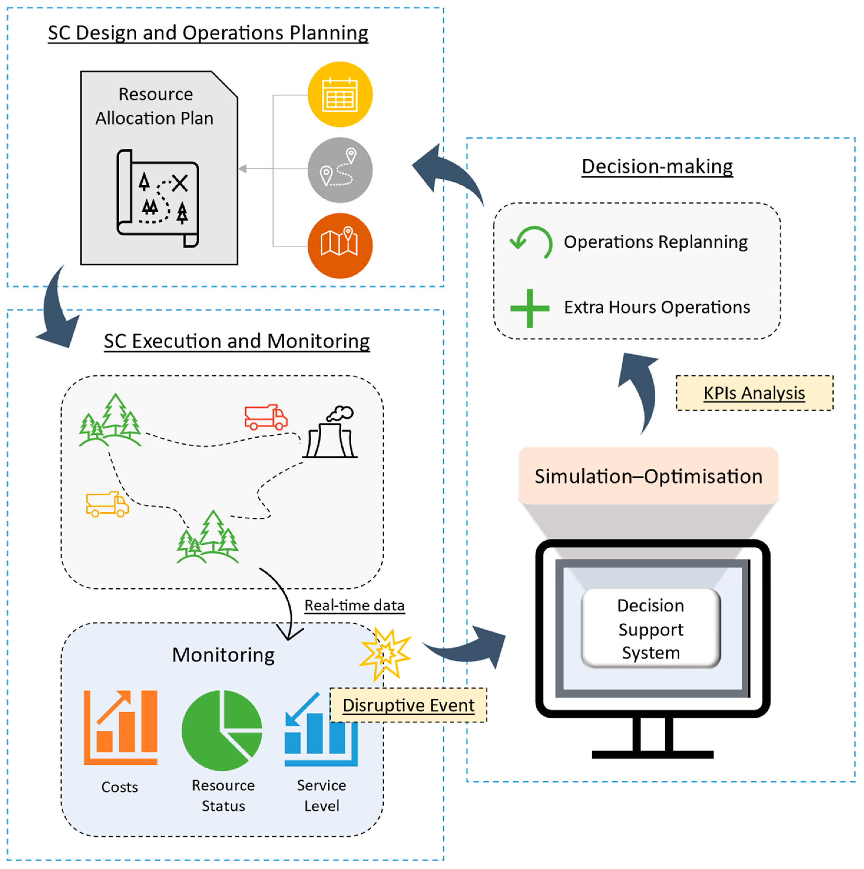
The architecture of the system developed in this work is sketched in Figure 2. Its main component is a decision support tool or system (DSS), that helps the decision-maker choose the best SC design and decide the day-to-day operations to perform along the SC. Moreover, the system was developed to be easily scalable and able to be used in other sectors and industries.

The developed DSS component encompasses a simulation/optimization integrated procedure that supports the construction of mitigation plans to maximise the amount of processed biomass. The system/decision-making process is organized as follows:

The initial optimisation model will generate three resource allocation plans. Each plan defines all the operations and biomass transportation actions to be performed during the planning horizon and will serve as input to the simulation model.

Periodically or with human intervention, the simulation model can be triggered using data coming from real-time execution and monitoring, containing a snapshot of all the biomass and resources flow along the chain. The simulation model checks and evaluates the disruptions impacts during the planning horizon, thus evaluating the robustness of the pre-allocated plan throughout time.

A trigger system is initiated if a disruption occurs. Based on simulation/optimisation key performance indicators (KPIs), the decision-maker selects what replanning method is used to mitigate the effects in the supply chain. Two types mitigation strategies of replanning procedures were defined: (a) related to extra operations and extra hours, without changing the initial resource allocation plan; (b) replanning using the optimisation model to obtain a new allocation plan for the remaining planning horizon.

With new changes to the original allocation plan, the process loop is closed and the steps above are continuously performed until the end of the time horizon.

The following sections present the optimisation and the simulation models in detail, analysing their potential, strengths, and limitations.

3.2. Resource Allocation Model

This section outlines the mathematical programming formulation developed for the supply chain network design problem. We have adopted a two-stage stochastic model based on a formulation of a working paper presented by [39]. Even if this formulation is not part of the current research, we present it here and explain its role on our methodological framework. Moreover, the model has undergone some changes to integrate replanning, taking into account the actual state of the chain and the occurrence of disruptions.

The model is based on a facility location problem with resource allocation. It considers a set of supply nodes to meet the demand of delivery nodes and includes a new echelon in this supply chain, the terminal nodes, that can store processed material from supply nodes. Decisions are related to where to process (supply nodes or terminals), when to process, for how long, and which machine (chipper) is allocated to perform these operations.

The model provides a set of operational plans by allocating teams and machines to the several supply nodes, to process the raw material needed to satisfy the monthly orders from the delivery nodes. These plans define the number of hours worked by each team and machine, the flows of processed and unprocessed material, and stock decision variables that guarantee the conservation of flows over time.

In addition to the previous parameters, there are parameters related to strategic-tactical decisions, such as the availability of the material in supply nodes, the demand in delivery nodes, and the possibility of opening terminal nodes. The short-term decisions are integrated into medium-term decisions to ensure the feasibility of solutions. All these decisions will be evaluated for a set of scenarios, related to a disruptive event that occurs in the supply chain.

The decision variables, sets, and parameters are presented first, followed by the objective function and the model constraints.

Sets

$P$	Set of raw material piles at the roadside
$M$	Set of power plants/mills
$O$	Set of terminals for raw material storage and chipping
$A$	Set of possible arcs, $A\left[P,O\right]=\left\{\left(p,o,l,c\right):\mathrm{p}\in P,o\in O,l\in \mathrm{L},\mathrm{c}\in \mathrm{C}\right\};$ $A\left[P,M\right]=\left\{\left(p,m,l,c\right):\mathrm{p}\in P,m\in \mathrm{M},l\in \mathrm{L},\mathrm{c}\in \mathrm{C}\right\};A\left[O,M\right]=\left\{\left(o,m,l,c\right):\mathrm{o}\in \mathrm{O},m\in \mathrm{M},l\in \mathrm{L},\mathrm{c}\in \mathrm{C}\right\},$ $A=A\left[P,O\right]\cup A\left[P,M\right]\cup A\left[O,M\right]$
$K$	Set of machines
$I$	Set of possible allocations, $I=\{\left(k,\mathrm{i},l,m\right):\mathrm{k}\in \mathrm{K},\mathrm{i}\in \mathrm{P}\cup \mathrm{O},\mathrm{l}\in \mathrm{L},\mathrm{c}\in \mathrm{C}\}$
$T$	Set of macro-periods for example months, $T=\{1,\dots ,\omega \}$
$L$	Set of micro-periods for example days, i = 1, …, $\omega ;L\left(i\right)=L\left(1\right)\cup \dots \cup L\left(\omega \right)$, where L(i) is the set of micro-periods of macro-period i, for i $\in \{1,\dots ,\omega \}$
$C$	Set of scenarios

Decision variables (first stage)

$\begin{array}{ll}{y}_o & \left\{\begin{array}{ll}1& \mathrm{if} \mathrm{terminal} \mathrm{node} o\in O \mathrm{is} \mathrm{open};\\ 0& \mathrm{otherwise}.\end{array}\right.\\ q_k & \left\{\begin{array}{ll}1& \mathrm{if} \mathrm{machine} k\in K \mathrm{is} \mathrm{used};\\ 0& \mathrm{otherwise}.\end{array}\right.\end{array}$

Decision variables (second stage)

$$\begin{array}{cc}\hfill x_{kilc} & \left\{\begin{array}{ll}1& \mathrm{if} \mathrm{machine} k\in K \mathrm{is} \mathrm{present} \mathrm{at} \mathrm{location} i\in S \mathrm{in} \mathrm{microperiod} l\in L\\ & \mathrm{in} \mathrm{scenario} c\in C;\\ 0& \mathrm{otherwise}.\end{array}\right.\hfill \\ \hfill z_{kilc} & \left\{\begin{array}{ll}1& \mathrm{if} \mathrm{machine} k\in K \mathrm{was} \mathrm{deployed} \mathrm{at} \mathrm{location} i\in S \mathrm{in} \mathrm{microperiod} l\in \mathrm{L}\\ & \mathrm{in} \mathrm{scenario} c\in C;\\ 0& \mathrm{otherwise}.\end{array}\right.\hfill \\ \hfill f_{ijlc} & \mathrm{flow} \mathrm{of} \mathrm{processed} \mathrm{material} \mathrm{traversing} \mathrm{arc} \left(i,j,l,c\right)\in A\left(ton\right)\hfill \\ & \\ \hfill e_{polc} & \mathrm{flow} \mathrm{of} \mathrm{raw} \mathrm{material} \mathrm{from} \mathrm{supply} \mathrm{node} p\in P \mathrm{to} \mathrm{terminal} o\in O \mathrm{in}\hfill \\ \hfill & \mathrm{microperiod} l\in \mathrm{L} \mathrm{in} \mathrm{scenario} c\in C \left(\mathrm{ton}\right)\hfill \\ \hfill r_{omlc} & \mathrm{flow} \mathrm{of} \mathrm{processed} \mathrm{material} (\mathrm{in} \mathrm{supply} \mathrm{node} p\in P) \mathrm{from} \mathrm{terminal}\hfill \\ \hfill & o\in O \mathrm{to} \mathrm{delivery} \mathrm{node} m\in M \mathrm{in} \mathrm{microperiod} l\in \mathrm{L} \mathrm{in} \mathrm{scenario} c\in C \left(\mathrm{ton}\right)\hfill \\ \hfill h_{kilc} & \mathrm{number} \mathrm{of} \mathrm{hours} \mathrm{worked} \mathrm{by} \mathrm{machine} k\in K \mathrm{at} \mathrm{location} i\in S \mathrm{in} \mathrm{microperiod}\hfill \\ \hfill & l\in \mathrm{L} \mathrm{in} \mathrm{scenario} c\in C\hfill \\ \hfill hextr{a}_{kilc} & \mathrm{number} \mathrm{of} \mathrm{extra} \mathrm{hours} \mathrm{worked} \mathrm{by} \mathrm{machine} k\in K\hfill \\ \hfill & \mathrm{at} \mathrm{location} i\in S \mathrm{in} \mathrm{microperiod} l\in L \mathrm{in} \mathrm{scenario} c\in C\hfill \\ \hfill s_{olc} & \mathrm{quantity} \mathrm{of} \mathrm{unprocessed} \mathrm{material} \mathrm{at} \mathrm{terminal} o\in O \mathrm{in} \mathrm{the} \mathrm{end} \mathrm{of}\hfill \\ \hfill & \mathrm{microperiod} l\in L \mathrm{in} \mathrm{scenario} c\in C \left(\mathrm{ton}\right)\hfill \\ \hfill v_{olc} & \mathrm{quantity} \mathrm{of} \mathrm{processed} \mathrm{and} \mathrm{stored} \mathrm{material} \mathrm{in} \mathrm{terminal} o\in O\hfill \\ \hfill & \mathrm{in} \mathrm{the} \mathrm{end} \mathrm{of} \mathrm{microperiod} l\in L \mathrm{in} \mathrm{scenario} c\in C \left(\mathrm{ton}\right)\hfill \\ \hfill w_{olc} & \mathrm{quantity} \mathrm{of} \mathrm{processed} \mathrm{material} \mathrm{in} \mathrm{supply} \mathrm{node} p\in P \mathrm{stored} \mathrm{in} \mathrm{terminal}\hfill \\ \hfill & o\in O \mathrm{in} \mathrm{the} \mathrm{end} \mathrm{of} \mathrm{microperiod} l\in L \mathrm{in} \mathrm{scenario} c\in C \left(\mathrm{ton}\right)\hfill \end{array}$$

Parameters (deterministic)

$$\begin{array}{cc}\hfill b_o & \mathrm{storage} \mathrm{capacity} \mathrm{at} \mathrm{terminal} o\in O\left(ton\right)\hfill \\ \hfill g_{mt} & \mathrm{demand} \mathrm{of} \mathrm{processed} \mathrm{material} \mathrm{at} \mathrm{delivery} \mathrm{node} m\in M\left(ton\right) \mathrm{in} \mathrm{macro}-\mathrm{period} t\in T\hfill \\ \hfill r_k & \mathrm{machine} \mathrm{productivity} k\in K\left(ton/h\right)\hfill \\ \hfill \psi & \mathrm{productivity} \mathrm{conversion} \mathrm{ratio}\hfill \\ \hfill d_{po} & \mathrm{travel} \mathrm{distance} \mathrm{from} p\in P \mathrm{to} o\in O \left(\mathrm{km}\right)\hfill \\ \hfill d_{pm} & \mathrm{travel} \mathrm{distance} \mathrm{from} p\in P \mathrm{to} m\in M \left(\mathrm{km}\right)\hfill \\ \hfill d_{om} & \mathrm{travel} \mathrm{distance} \mathrm{from} o\in O \mathrm{to} m\in M \left(\mathrm{km}\right)\hfill \\ \hfill \gamma & \mathrm{conversion} \mathrm{ratio} \mathrm{of} \mathrm{the} \mathrm{transport} \mathrm{capacity} \mathrm{of} \mathrm{a} \mathrm{truck} \mathrm{with} \mathrm{unprocessed} \mathrm{material}\hfill \\ \hfill q & \mathrm{transport} \mathrm{capacity} \mathrm{of} \mathrm{a} \mathrm{truck} \mathrm{with} \mathrm{processed} \mathrm{material} \left(ton\right)\hfill \\ \hfill {\alpha }_{ki} & \mathrm{hourly} \mathrm{working} \mathrm{cost} \mathrm{for} \mathrm{machine} k\in K (€) \mathrm{at} \mathrm{location} i\in S\hfill \\ \hfill s & \mathrm{truck} \mathrm{distance} \mathrm{cost} (€/km)\hfill \\ \hfill \omega & \mathrm{end} \mathrm{of} \mathrm{planning} \mathrm{horizon}\hfill \\ \hfill c_k & \mathrm{cost} \mathrm{of} \mathrm{selecting} \mathrm{machine} k\in K\hfill \\ \hfill \tau & \mathrm{total} \mathrm{working} \mathrm{time} \mathrm{per} \mathrm{microperiod} l\in L\hfill \\ \hfill {\sigma }_o & \mathrm{cost} \mathrm{of} \mathrm{opening} \mathrm{a} \mathrm{terminal} o\in O (€)\hfill \\ \hfill {\beta }_i & \mathrm{cost} \mathrm{of} \mathrm{machine} \mathrm{deploying} \mathrm{to} \mathrm{location} i\in S (€)\hfill \end{array}$$

Parameters (stochastic)

$$\begin{array}{cc}\hfill p_c & \mathrm{probability} \mathrm{of} \mathrm{occurrence} \mathrm{of} \mathrm{scenario} c\in C\hfill \\ \hfill a_{ptc} & \mathrm{availability} \mathrm{of} \mathrm{raw} \mathrm{material} \mathrm{in} \mathrm{supply} \mathrm{node} p\in P\left(ton\right) \mathrm{in} \mathrm{macroperiod} t\in T\hfill \\ \hfill & \mathrm{in} \mathrm{scenario} c\in C\hfill \\ \hfill A_{ptc} & ={\displaystyle \sum _{t^{\prime }\in T:t^{\prime }\le t}}\Vert a_{ptc}\hfill \end{array}$$

Some parameters used in this formulation are transversal to any business and others are specific to the forest biomass supply chain. Trucks with unchipped material cannot carry the same load weight, as this type of material occupies three times more volume than chips, resulting in the use of a conversion ratio of the transport capacity of a truck with unprocessed material, parameter $\left(\gamma \right)$. Productivity conversion ratio $\psi$ reflects productivity losses related to road slope, quantity of material, set-up times, and location access. Since the cost per kilometer of transporting a machine from one location to another is not very high when compared to the costs of loading, unloading, and set-up of the machines, an average cost per deployment of a machine of one location to another (i.e., from one terminal to another terminal) was considered. Some parameters vary across the planning horizon. That is the case, for example, of the quantity available in a pile throughout the time periods, and the demand during the planning horizon. The model is sufficiently comprehensive to be easily adapted to other supply chains. 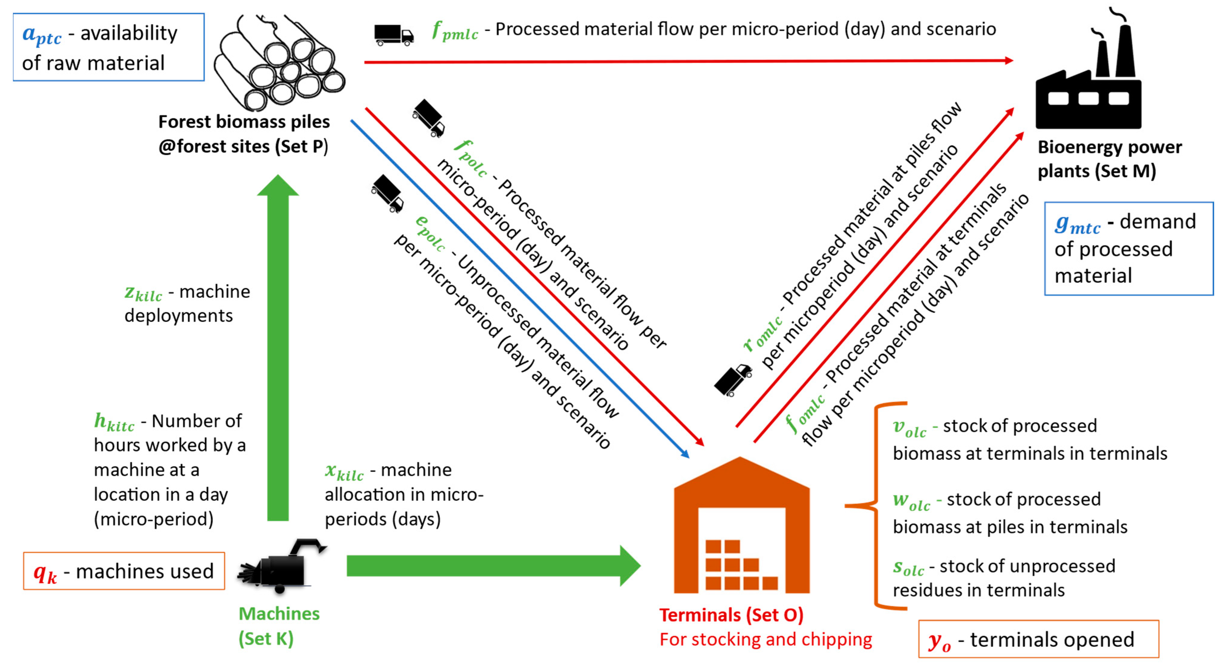Figure 3 presents the biomass logistics supply chain, along with the decision variables and the parameters associated with the operations.

Objective Function

$$\begin{array}{rr}& \mathrm{m}\mathrm{i}\mathrm{n}\\ & ({\displaystyle \sum _{\left(i,j,l,c\right)\in A}}\frac{d_{ij}\cdot s\cdot f_{ijlc}}{q}\\ & +{\displaystyle \sum _{\left(p,o,l,c\right)\in A:\left[P,O\right]}}\frac{d_{po}\cdot s\cdot e_{polc}}{q\cdot \gamma }\\ & +{\displaystyle \sum _{\left(o,m,l,c\right)\in A:\lceil O,M]}}\frac{d_{om}\cdot s\cdot r_{omlc}}{q}\\ & +{\displaystyle \sum _{o\in O}}{\sigma }_o\cdot y_o+{\displaystyle \sum _{k\in K}}{c}_k\cdot q_k\\ & +{\displaystyle \sum _{\left(k,i,l,c\right)\in I}}{\beta }_i\cdot z_{kilc}\\ & +{\displaystyle \sum _{\left(k,i,l,c\right)\in I}}{\alpha }_{ki}\cdot (h_{kilc}+hextr{a}_{kilc}))\cdot p_c\end{array}$$

(1)

The objective function was designed to minimise total costs: the costs of transporting processed and unprocessed material between the different nodes; the monthly cost of opening and keeping the terminal nodes open; the cost of deploying a machine in a given location; and finally, the processing costs, that depend on the working hours of each machine. This stochastic model generates a plan involving the strategic decisions related to opening terminals and the machines to be used. This model is run with a set of scenarios with an associated probability of occurrence. This way, the objective function also considers the probability of occurrence of each scenario $(p_c$). In the specific case of considering only one scenario, the probability of occurrence of this scenario will be 100%, thus the parameter is always considered, and cannot be zero.

Constraints

$$\begin{gathered} \sum _{\left(o,l\right):\left(p,o,l,c\right)\in A\left[P,O\right]\wedge l\in \mathrm{L}\left(1\right)\cup \dots \cup L\left(t\right)}{f}_{polc}+\sum _{\left(m,l\right):\left(p,m,l,c\right)\in A\left[P,M\right]\wedge l\in \mathrm{L}\left(1\right)\cup \dots \cup L\left(t\right)}{f}_{pmlc}+ \\ \sum _{\left(o,l\right):\left(p,o,l,c\right)\in A\left[P,O\right]\wedge l\in \mathrm{L}\left(1\right)\cup \dots \cup L\left(t\right)}{e}_{polc}\le A_{ptc}, \forall p\in P,\forall t\in T \end{gathered}$$

(2)

$$s_{olc}+v_{olc}+w_{olc}\le b_o, \forall o\in O,\forall l\in L$$

(3)

$$\begin{gathered} {\sum }_{\left(p,l\right):\left(p,m,l,c\right)\in A\left[P,M\right]\wedge l\in \mathrm{L}\left(1\right)\cup \dots \cup L\left(t\right)}{f}_{pmlc}+ \\ {\sum }_{\left(o,l\right):\left(o,m,l,c\right)\in A\left[O,M\right]\wedge l\in \mathrm{L}\left(1\right)\cup \dots \cup L\left(t\right)}{f}_{omlc}+ \\ {\sum }_{\left(o,l\right):\left(o,m,l,c\right)\in A\left[O,M\right]\wedge l\in \mathrm{L}\left(1\right)\cup \dots \cup L\left(t\right)}{r}_{omlc}\ge g_{mtc}, \forall m\in M,\forall t\in T \end{gathered}$$

(4)

$$\sum _{i:\left(k,i,l,c\right)\in I}{x}_{kilc}\le 1, \forall k\in K,\forall l\in L$$

(5)

$$\sum _{k:\left(k,p,l,c\right)\in I}{x}_{kplc}\le 1, \forall p\in P,\forall l\in L$$

(6)

$$f_{pmlc}\le A_{ptc}\sum _{k\in K:\left(k,p,l,c\right)\in I}{x}_{kplc},\forall \left(p,m,l,c\right)\in A[P,M],l\in \mathrm{L}\in T,\forall t\in T$$

(7)

$$f_{ojlc}\le b_o,\forall \left(o,j,l,c\right)\in A:o\in O$$

(8)

$$f_{polc}\le b_o{y}_o, \forall \left(p,o,l,c\right)\in A:p\in P,o\in O$$

(9)

$$r_{ojlc}\le b_o{y}_o, \forall \left(o,j,l,c\right)\in A:o\in O$$

(10)

$$h_{kilc}\le x_{kilc}\tau \forall \left(k,i,l,c\right)\in I$$

(11)

$$hextr{a}_{kilc}\le x_{kilc}\tau \forall \left(k,i,l,c\right)\in I$$

(12)

$$\sum _{k\in K:(k,p,l,c)\in I}{h}_{kplc}\ge \sum _{m\in M:\left(p,m,l,c\right)\in A}\frac{f_{pmlc}}{r_k\cdot \psi } \forall p\in P,\forall l\in L$$

(13)

$$z_{kilc}\ge x_{kilc}-x_{ki\left(l-1\right)c} \forall \left(k,i,l,c\right)\in I$$

(14)

$$z_{ki0\mathrm{c}}\ge x_{ki0\mathrm{c}} \forall \left(k,i,\left(0\right),c\right)\in I$$

(15)

$$n\cdot y_o\ge \sum _{k\in K:\left(k,o,l,c\right)\in I,l\in L}{x}_{kolc} \forall o\in O,\forall t\in T$$

(16)

$$s_{olc}=s_{o\left(l-1\right)c}+\sum _{p\in p:\left(p,o,l,c\right)\in A[P,O]}{e}_{polc}-\sum _{k\in K:\left(k,o,l,c\right)\in I}\left(h_{kolc}+hextr{a}_{kolc}\right)r_k \forall o\in O,\forall l\in L$$

(17)

$$s_{o\left(0\right)c}=\sum _{p\in P:\left(p,o,\left(0\right),c\right)\in A[P,O]}{e}_{po\left(0\right)c}-\sum _{k\in K:\left(k,o,\left(0\right),c\right)\in I}\left(h_{ko\left(0\right)c}+hextr{a}_{ko\left(0\right)c}\right)r_k \forall o\in O,\forall c\in C$$

(18)

$$v_{olc}=v_{o\left(\mathrm{t}-1\right)c}+\sum _{k\in K:\left(k,o,l,c\right)\in I}\left(h_{kolc}+hextr{a}_{kolc}\right)r_k-\sum _{m\in M:\left(o,m,l,c\right)\in A[O,M]}{f}_{omlc} \forall o\in O,\forall l\in L,\forall c\in C$$

(19)

$$v_{o\left(0\right)c}=\sum _{k\in K:\left(k,o,\left(0\right),c\right)\in I)}\left(h_{ko\left(0\right)c}+hextr{a}_{ko\left(0\right)c}\right)r_k-\sum _{m\in M:\left(o,m,\left(0\right),c\right)\in A[O,M]}{f}_{om\left(0\right)c} \forall o\in O,\forall c\in C$$

(20)

$$w_{olc}=w_{o\left(t-1\right)c}+\sum _{p\in P:\left(p,o,l,c\right)\in A[P,O]}{f}_{polc}-\sum _{m\in M:\left(o,m,l,c\right)\in A[O,M]}{r}_{omlc} \forall o\in O,\forall c\in C$$

(21)

$$w_{o\left(0\right)c}=\sum _{p\in P:\left(p,o,\left(0\right),c\right)\in A[P,O]}{f}_{po\left(0\right)c}-\sum _{m\in M:\left(o,m,\left(0\right),c\right)\in A[O,M]}{r}_{om\left(0\right)c} \forall o\in O,\forall c\in C$$

(22)

$$\sum _{\left(o,l\right):\left(p,\mathrm{o},l,c\right)\in A\left[P,O\right]\wedge l\in L}{f}_{polc}+\sum _{\left(m,l\right):\left(p,m,l,c\right)\in A\left[P,M\right]\wedge l\in L}{f}_{pmlc}+\sum _{\left(o,l\right):\left(p,o,l,c\right)\in A[P,O]l\in \mathrm{L}}{e}_{polc}=A_{p\omega c}, \forall p\in P,\forall c\in C$$

(23)

$$x_{kilc},z_{kilc},q_{k,}{y}_{o,}\in \left[\mathrm{0,1}\right]$$

(24)

$$f_{ijlc},e_{polc},r_{omlc},h_{kilc},hextr{a}_{kilc},s_{olc},v_{olc},w_{olc}\ge 0$$

(25)

The model is basically a facility location problem (FLP), in which a set of supply nodes was selected to meet the demand of delivery nodes. For this purpose, the model needs to ensure that the following constraints are fulfilled: the flow leaving supply nodes cannot exceed its availability (Constraint (2)); capacity at terminal nodes (Constraint (3)); demand satisfaction (Constraint (4))—the flow from processing nodes in each time period meets the demand of delivery nodes in that time period.

The model also includes constraints related to the assignment of machines. It is not possible to have the same machine allocated to two or more locations on the same day (micro period) (Constraint (5)), and no more than one machine may be present on the same supply node at the same time (Constraint (6)). There is only a flow of processed material from a supply node to another node, only when at least one machine is in this supply node (Constraint (7)). There is only a flow of processed material in the terminal node from a terminal node to a power plant when some machine is present in this terminal node (Constraint (8)).

The number of processing hours is upper bounded by the duration of the micro period (day) working time (Constraints (11) and (12)); the number of processing hours of a specific machine in a supply node is greater than or equal to its processing productivity of raw material (Constraint (13)); the conversion ratio $\psi$ reflects productivity losses related to road slope, the quantity of material and location access. Constraints (14) and (15) ensure that there is only one machine deployment from one place to another in a given micro period, and guarantee that a deployment is only accountable when a machine change location in the next micro-period. This means that there has only been a machine deployment if the terminal where the machine is currently working is different from where it was working the prior day.

Constraints (9), (10), and (16) account for the possibility of opening a terminal node. A terminal node must be open if flows occur from a terminal node and/or there is machine allocated to it. There will not be any machine allocation $\left(x_{kol}\right)$ or flow $\left(r_{oml}\right)$ for the duration of each time period $\left(y_o\right)$, if there is not a terminal node available and ready to receive biomass in that time period. Constraints (17)–(22) assure flow conservation by stock constraints. Constraint (23) ensure that at the end of the planning horizon, all raw material available in each supply node must be processed, that is, transported to a destination node (processed or unprocessed). Finally, constraints (24) and (25) define the domain of the decision variables.

3.3. Simulation Model

The discrete event simulation (DES) model described in this paper was implemented using the FlexSim software 2023 (FlexSim Software Products, Orem, UT, USA) [40]. The model is integrated with a GIS system and with the previous described optimisation model, in order to analyse and compare the feasibility of various SC configurations and operations planning alternatives.

For the validation of the results obtained by using the pre-generated allocation plans as input of the simulation model, some previous work [41] was used as a basis. In this work, the supply chain setup in FlexSim was very similar to the previous work and included:

• Modelling of the network points (piles, terminals and power plants) on the FlexSim map, with the associated locations;
• Creation of the “chippers” and terminals established by the optimisation model;
• Data conversion from input files to data tables, concerning pile supply, power plants demand, processing times, deployments of machines, and transportation amounts of processed and unprocessed biomass from one location to another;
• Creation of routes connecting all network points.

Before running the simulation model, resource allocation plans are automatically loaded on FlexSim data tables. After the network setup, the execution includes the operation of resources and biomass flow, i.e., the transportation of the “chippers”, the “chipping” process, and the transportation of processed or unprocessed biomass from piles to terminals and to the bioenergy power plants.

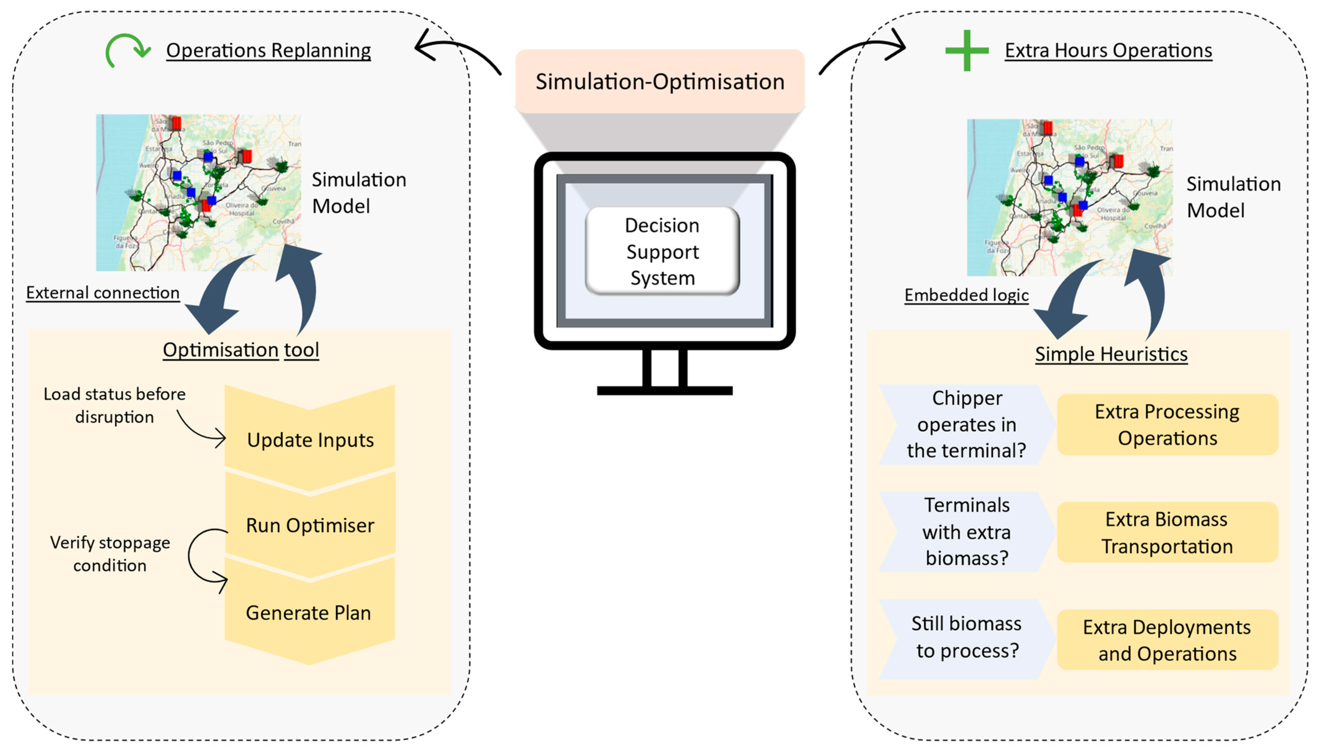
The replanning method includes the trigger system explained above, allowing the decision-maker to choose one of the two mitigation strategies. Figure 4 presents the simulation methodology of the DSS and the way the two strategies operate. The first one is related to adding extra operations to the initial plan, and the second strategy consists of a complete replanning of the operations in the supply chain, with the optimisation model previously developed.

3.3.1. Replanning with Simulation Embedded Heuristics

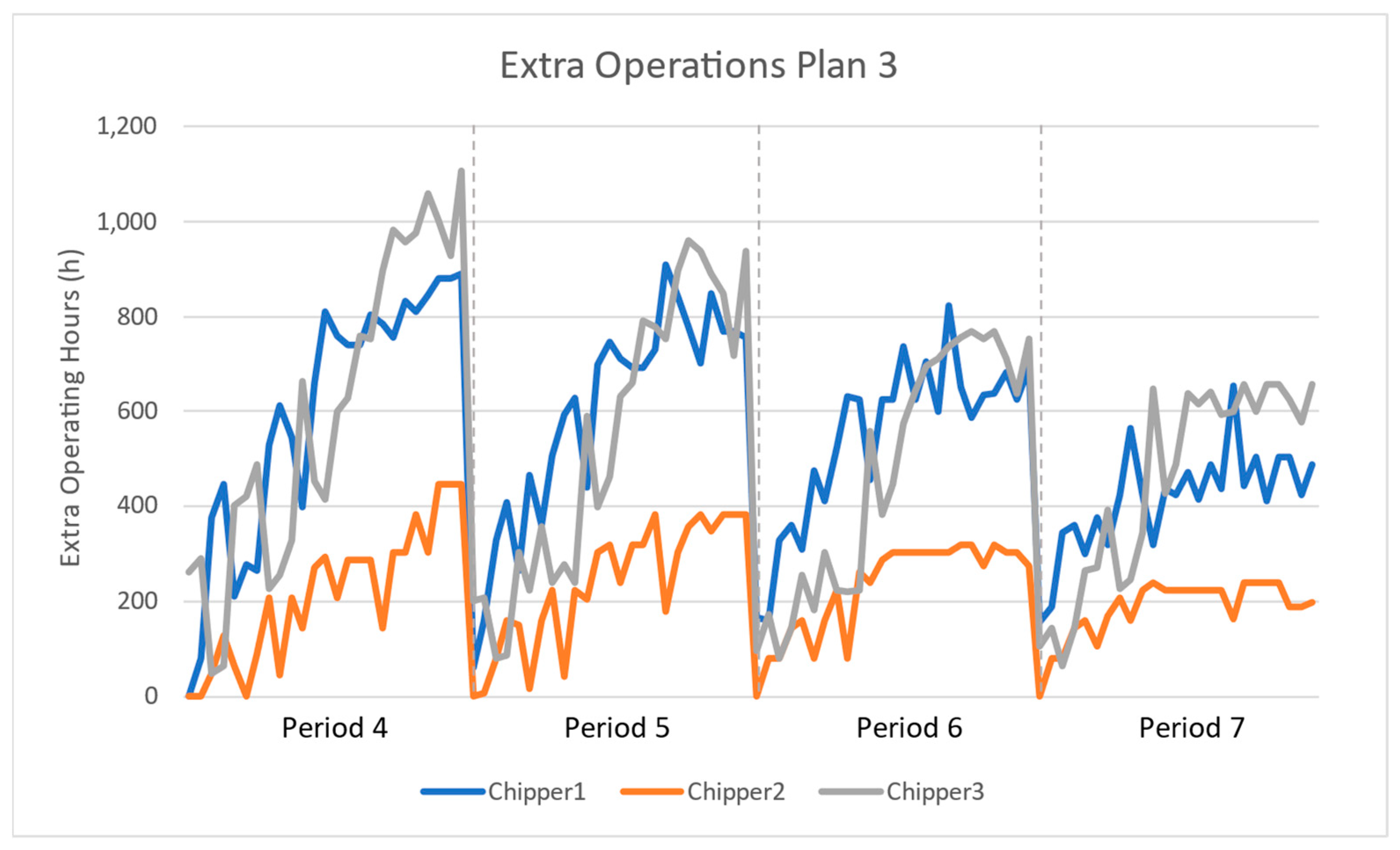
The first mitigation strategy is related to replanning with simple heuristics. These heuristics add extra operations to the pre-defined plan if certain conditions occur. For this purpose, several steps are performed. The first step is to determine whether chippers are already in operation at the terminal; if so, further processing can occur in the same day, utilising extra hours. The second step is to determine if the current processed biomass in the terminal is sufficient to fulfil demand; if so, an additional order of transportation is triggered by transferring biomass from the terminal to the power plant. Finally, if there is still biomass to process, five days at the end of each month can hold extra chippers’ deployments and processing. In this case, each chipper can only be deployed once (the first available chipper is deployed at the terminal and operates up to 16 extra hours each day until the end of the month).

3.3.2. Replanning with Simulation/Optimisation

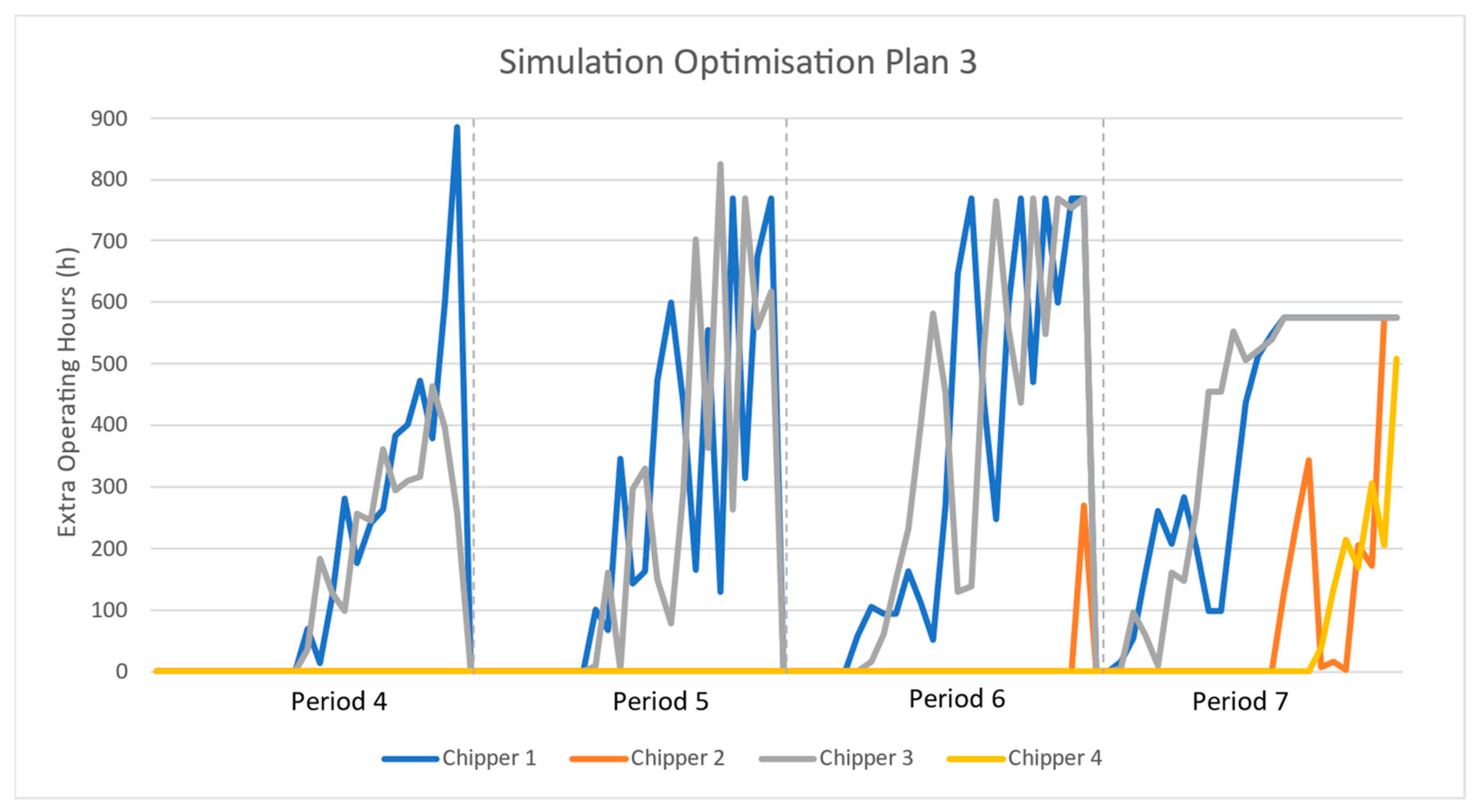
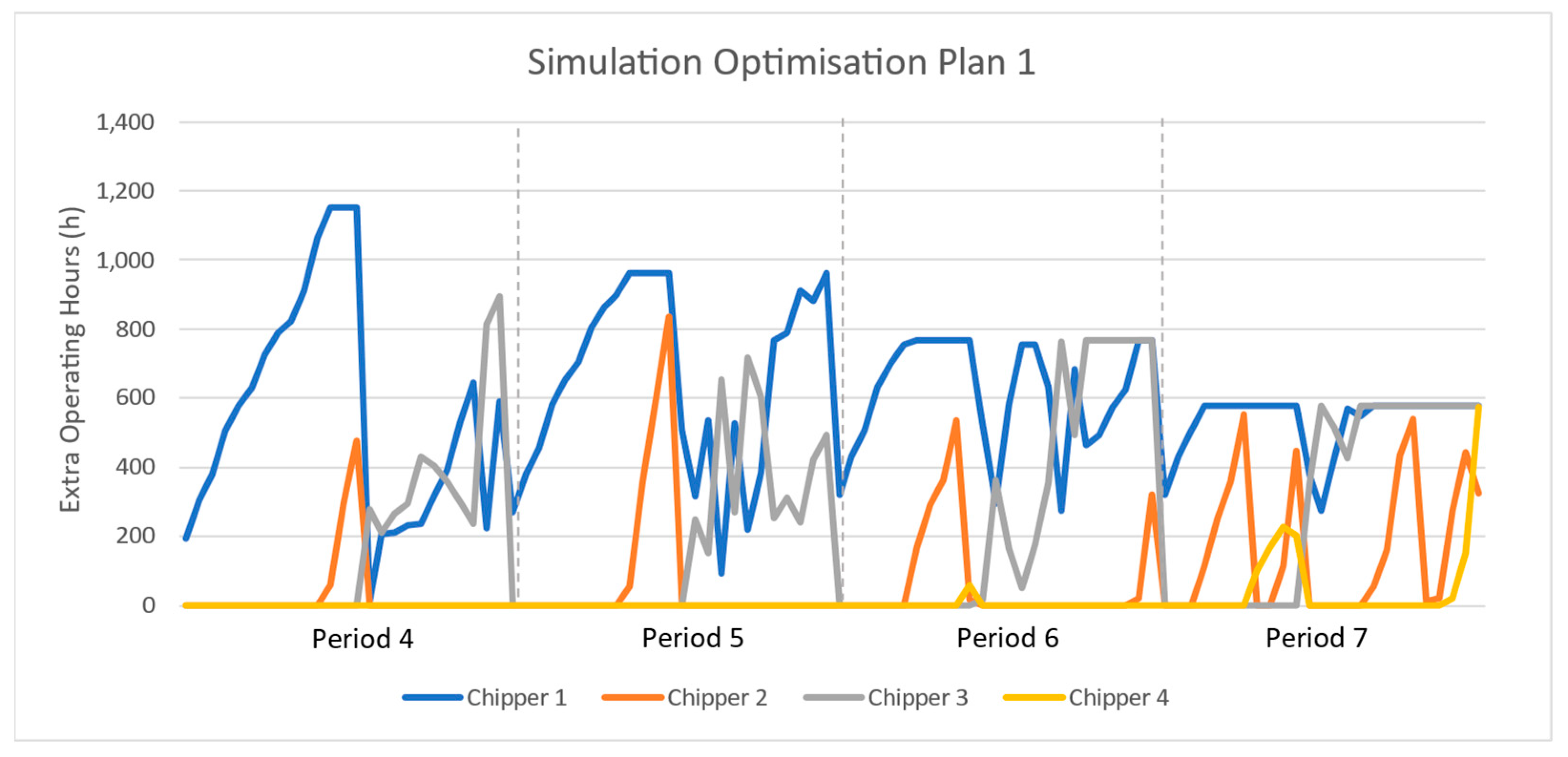
The second mitigation strategy is related to the optimisation model and takes advantage of an external connection to python, to determine a new resource allocation plan after the disruption event occurs. This hybrid approach will replan all the operations and processes of the remaining months, disregarding the initial plan. This includes:

• The creation of a JSON file with the information on the biomass SC after the disruption has occurred; the file contains the “chippers” location, the amount of biomass to process in the terminals, the demand to fulfil in each power plant and the biomass in each pile;
• A call of the optimisation model (developed using python) with the JSON file as input through FlexSim (the overall process uses the FlexSim interface and connections);
• Running the optimisation model to obtain a new resource allocation plan with available chippers and terminals;
• A FlexSim new setup, using a new replanning data table and associated routes;
• The identification and update of new terminals and chippers to buy, adding them to the model.

After the modelling phase, a parameters data table is also used for testing and assessing alternatives. The execution of the base model starts when the network configuration and scenario description have been completed. Dynamic dashboards collect performance metrics to be analysed by the planners.

4. Case Study

Section 4.1 describes the case study used in this work. Section 4.2 presents the process to generate the scenarios that were tested in this approach.

4.1. Case Study

A realistic case study [41] was designed based on a biomass supplier company running a supply chain (SC) in Portugal. The company is responsible for “chipping” and transporting wood chips to fulfil the power plant’s expected monthly demand. The company agrees to supply a certain amount of processed biomass to each power plant once a month.

For this purpose, the company makes contracts with forest owners who provide locations with forest residues for the biomass production, known as piles. Forest residues are about 30% of all wood harvest in the logging industry (specially pine and eucalyptus). These residues (slabs, branches, and barks removed from tress) are transported to the forest roadside, to make them more accessible to trucks and chippers. In addition, the piles are geographically dispersed all over the region, as there are many harvesting locations to include in the operation plans.

An operations planning horizon of nine months is considered (going from March to November) thus avoiding operations in rainy periods. However, the summer period directly affects SC planning due to the risk of fires. Each month is assumed to have 24 working days, and each day has eight hours of regular work (one shift) and the possibility of eight hours of extra work (a second shift).

Two types of resources were considered in this case study: trucks and “chippers”. The “chippers” are responsible for processing the forest residues and can be deployed at different locations. The maximum number of available “chippers” is limited to four. The company has already acquired two chippers, and two other chippers can be acquired later, either at the beginning of the year at a lower price, or during the year at a higher but fixed price.

There is no bound on the number of trucks that can be used in moving the biomass from one node to another. It is important to note that the volume of the processed biomass will be reduced by nearly three times, making the biomass processing ratio around 0.3. Due to the volume, each truck has a capacity of 25 tonnes for chipped material but only 8 tonnes for unprocessed biomass. For this specific case study, trucks were the chosen transport mode because the supply chain area is quite small and the biomass harvesting locations are difficult to access by other transport methods.

The company can also acquire some terminals over the planning horizon or, as an alternative, can hire a maximum of 5 terminals, in the beginning. Terminal 1 is always hired because it is where the “chippers” are stored. These terminals are used both to perform the chipping operations and to store the biomass.

Two decision levels are considered: “short-term” and “long-term”, associated to months and days, respectively. For the 9 months of operation, the company wants to define how many piles (location of the feedstock) should be used, and how many “chippers” and terminals should be operating and purchased. The day-to-day planning includes deploying and assigning the “chippers” to the piles and terminals, choosing the routes for transporting biomass, and deciding how many hours the “chippers” will operate daily. However, these plans will change in case a disruption occurs, and if there are changes in the supply or in the demand.

Earlier research [41] has suggested that processing biomass only at terminals would have better results in a real-world context, helping to prevent disruptive events and associated undesired results. It was also possible to conclude that if all the biomass is processed, the SC is better prepared to handle variations in both supply and demand. Based on this know-how, three plans were defined, assuming that biomass processing could only occur in terminals and had to be fully processed.

Therefore, the difference between plans is related to the number of “chippers” in operation and their capacity to process biomass hourly.

Table 1. Chippers production capacity and chippers used by each plan.

	Production Capacity (Tons/Hour)	Plan 1	Plan 2	Plan 3
Chipper 1	20	x	x	x
Chipper 2	10	x		x
Chipper 3	20		x	x
Chipper 4	10

shows the “chippers” included in each plan and their production capacity. Plan 1 is based on “chippers” 1 and 2, already acquired by the company, thus implying no investment. Plans 2 and 3 use “chipper” 3, yielding therefore an investment in a new chipper. In addition, Plan 3 also uses “chipper” 2, mainly if a disruption occurs.

However, as mentioned earlier, it is possible to purchase “chippers” or terminals somewhen during the planning horizon. There are two types of purchase. A “chipper” can be bought at the beginning of the planning horizon, and is paid in instalments throughout the year, even if not used. Or, as an alternative, it can be bought in the middle of the year, which means a unique payment. The same happens for terminals.

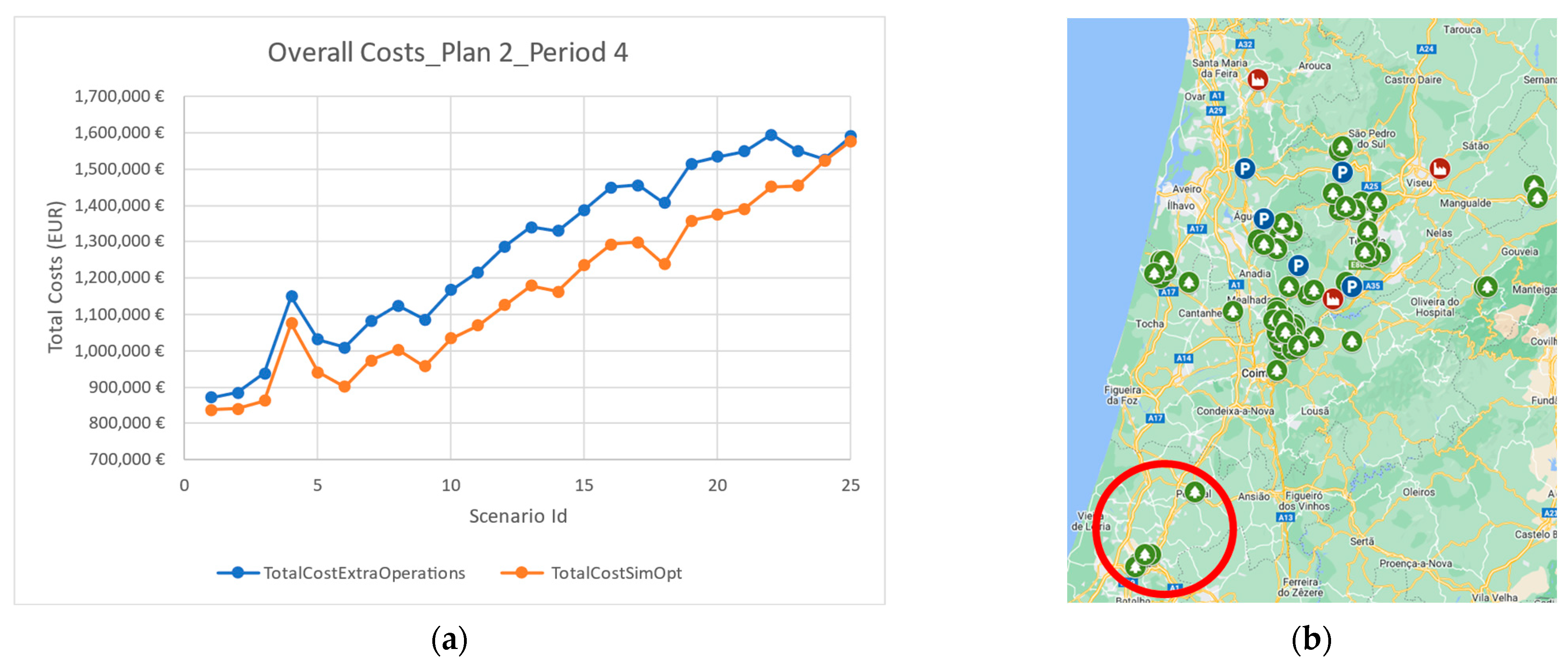
Figure 5 represents the current logistics network composed of 64 wood piles (points in green), three bioenergy plants (points in red), and finally, five possible locations for terminals (points in blue). Figure 5a gives a visual representation of a supply chain map, and the data of the case study in the simulation model is presented in Figure 5b.

4.2. Generation of Scenarios

As previously mentioned, in this work, a series of scenarios was defined to represent disruptive events occurring in the biomass supply chain. For this study, the occurrence of a fire in the forest was the disruption considered. A forest fire is a common and unpredictable situation that can lead to a significant increase of the amount of unprocessed biomass in the piles. This increase happens because biomass residues come mainly from the wood industry, so if the wood is completely burned companies cannot use it, and therefore, more residues have to be used in the biomass industry. Furthermore, the number of piles can increase, and the extra biomass must be transported and processed.

In this context, a scenario is defined by the number of piles affected by the fire that will generate different amounts of extra biomass. The piles impacted by the fire were generated using a fire propagation simulator proposed by [42] that accounts for the geography of the land, the winds, and the duration of the fire.

Table 2. Examples of scenarios with the number of piles affected by the fire and the amount of extra biomass generated.

Scenario ID	Piles Affected by the Fire (ID)	Number of Piles	Amount of Extra Biomass (Tons)
1	23; 28; 48; 59	4	5245
2	1; 3; 5; 14; 15	5	7430
3	10; 11; 38; 41; 44; 64	6	8959
4	51; 52; 53; 54; 55	5	11,505
5	14; 15; 23; 28; 48; 49; 56; 57; 58; 59	10	12,910
6	2; 3; 5; 12; 14; 15; 56	7	13,965
7	2; 3; 14; 15; 23; 28; 48; 49; 56; 57; 59	11	15,925
8	8; 9; 17; 18; 19; 20; 21; 25; 26; 40; 41; 43; 60; 61	14	17,150
9	3; 5; 12; 13; 29; 30; 31; 32; 35; 36; 37; 39; 50; 63	14	17,835
10	8; 9; 17; 18; 19; 20; 21; 22; 25; 26; 40; 41; 43; 60; 61; 62	16	19,580
11	1; 2; 3; 4; 14; 15; 23; 24; 28; 33; 34; 48; 49; 56; 57; 58; 59	17	22,650
12	7; 8; 9; 16; 17; 18; 19; 20; 21; 24; 25; 26; 33; 34; 40; 42; 43; 60; 61	19	24,995
13	6; 7; 8; 9; 17; 18; 19; 20; 21; 22; 25; 26; 40; 42; 43; 47; 51; 60; 61; 62	20	27,395
14	3; 5; 6; 7; 10; 11; 12; 16; 22; 27; 32; 33; 35; 38; 41; 44; 47; 62; 64	19	29,199
15	6; 7; 8; 9; 16; 17; 18; 19; 20; 21; 22; 24; 25; 26; 27; 34; 40; 42; 43; 47; 60; 61; 62	23	30,275
16	6; 7; 8; 9; 16; 17; 18; 19; 20; 21; 22; 23; 24; 25; 26; 27; 28; 34; 40; 42; 43; 48; 60; 61; 62	25	32,855
17	4; 6; 7; 8; 9; 16; 17; 18; 19; 20; 21; 22; 24; 25; 26; 27; 33; 34; 40; 41; 42; 43; 44; 47; 60; 61; 62	27	33,980
18	1; 2; 3; 4; 5; 6; 10; 11; 12; 13; 14; 15; 24; 27; 29; 30; 31; 32; 33; 34; 44; 47; 50; 62	24	35,005
19	1; 2; 3; 4; 5; 6; 7; 8; 9; 15; 16; 22; 24; 25; 26; 27; 28; 33; 34; 40; 41; 42; 43; 44; 47; 48; 56; 57; 59; 62	30	37,785
20	2; 3; 4; 6; 7; 8; 9; 11; 14; 15; 16; 22; 24; 25; 26; 27; 28; 33; 34; 40; 41; 42; 43; 44; 47; 48; 56; 58; 59; 62	30	38,825
21	1; 2; 3; 4; 6; 7; 8; 9; 11; 16; 17; 18; 20; 22; 24; 25; 26; 27; 33; 34; 40; 41; 42; 43; 44; 47; 48; 60; 61; 62	30	39,490
22	1; 2; 3; 4; 6; 7; 8; 9; 14; 15; 16; 22; 23; 24; 25; 26; 27; 28; 33; 34; 40; 42; 43; 47; 48; 49; 56; 57; 58; 59; 62	31	41,075
23	2; 3; 4; 6; 7; 8; 9; 10; 11; 16; 17; 18; 19; 20; 21; 22; 24; 25; 26; 27; 33; 34; 40; 41; 42; 43; 44; 47; 60; 61; 62	31	42,100
24	2; 4; 6; 7; 8; 9; 10; 11; 12; 16; 17; 18; 21; 22; 25; 26; 27; 33; 34; 38; 40; 41; 42; 43; 44; 47; 60; 61; 62; 64	30	45,144
25	1; 2; 3; 4; 6; 7; 8; 9; 10; 11; 12; 15; 16; 17; 18; 20; 21; 22; 24; 25; 26; 27; 33; 34; 40; 41; 42; 43; 44; 47; 48; 60; 61; 62	34	48,160

presents the 25 scenarios generated in this work. Scenario 1 starts with 5245 tons of extra biomass, this quantity being progressively increased until scenario 25, with 48,160 tons. The fire scenario is also defined by the period in which it occurs and by the forest age (adult or young).

5. Results

This section presents and analyses the results obtained for each scenario. In this context, the main purpose of the computational experiments is to evaluate the performance of the three generated plans, using the two considered mitigation approaches for replanning (extra operations, and simulation/optimisation) mainly based on the simulation results. These results should reflect the uncertainty and variability dimensions added by the occurrence of disruptions.

5.1. Analysis of Results

The proposed approach was tested in the case study, for all the scenarios. These tests were performed for the 3 plans, in 4 different periods associated to the months with higher probability of a fire occurrence. The “solver” used to build the mathematical model was Gurobi 10.0 (Gurobi Optimization, Houston, TX, USA), and Python 3.10 (The Python Software Foundation, Wilmington, DE, USA) was used set up and parametrise the model. FlexSim 2023 was used to create the simulation model.

A set of 600 simulation runs was generated, to provide significant management insights to planners, on the impacts of flexible planning in various circumstances. Three initial resource allocation plans were used, along with the two mitigation strategies described above.

5.1.1. Service Level

Figure 6 shows the average values of “service level” (the percentage of processed biomass in the total available biomass), with 25 scenarios separated by four periods, in a total of 100 scenarios (25 × 4). The “simulation/optimisation” led to better results than “adding extra operations”, in terms of service level, with all plans getting a value of 100% for all the periods.

In what concerns the performance of the plans, as expected, plans using more “chippers” or more capacity achieve better values of service level. This is well evidenced in Plan 3 (three available “chippers”), with the highest service level. Regarding the fire occurrence, the impact of extra operations decreases as the fire period gets closer to the end of the planning horizon. This is justified because the number of available hours to perform extra operations decreases throughout time, meaning less biomass is processed by “chippers”.

Although Plan 1 processes less biomass, it does not require any additional investment since the company already owns the two utilized “chippers”. This observation suggests we need to perform a more careful cost-benefit analysis.

5.1.2. Overall Costs

Regarding costs, Figure 7 shows the total SC costs (without considering penalty costs for not processing all available biomass) split by period (each with 25 scenarios) and using both mitigation strategies. In general, using the simulation/optimisation approach is more costly than using “extra operations” (simulation heuristics). However, comparing both strategies during period 4 for Plans 2 and 3, with simulation heuristics having a service level closer to 100% (see Figure 6), these heuristics have higher costs. This happens because, while this approach processes biomass only with overtime, the simulation/optimisation approach can replan all operations using fewer extra operations.

Furthermore, regarding the period of fire occurrence, as the fire duration increases, the costs of extra operations decrease and the costs of simulation/optimisation increase. As stated in the previous section, this deviation arises because the extra operations cannot process everything as the period increases and there is no penalty cost for unprocessed biomass. In addition, it is also possible to observe a similar result when using simulation/optimization for Plans 2 and 3. This can be justified because, in Plan 3, “chipper 2” is only reserved for emergencies, this leading to similar operations when compared with Plan 2, thus having similar costs.

An interesting fact is the almost linear correlation between scenarios and costs for the same period. Still, some deviations are evident. Figure 8a presents an example relating the total costs of the two mitigation strategies, for Plan 2 in period 4. Here, the main point to analyse is the peak associated to scenario 4, that is replicated for all periods, plans and mitigation strategies.

This situation occurred because scenario 4 had 5 piles affected by the fire located at the most southern part of the region (Figure 8b). Thus, these piles are very far away from the terminals, with an increase in transportation costs from the piles to the terminals.

5.1.3. “Chippers” Operation Overtime

Most of the costs are related to the overtime each “chipper” needs to process all the extra biomass, justifying, therefore, an analysis of how the extra hours of each “chipper” vary throughout the different periods.

Regarding the replanning options, the extra operating hours are higher on average in the simulation heuristics mitigation strategy than in the simulation/optimisation. This is easily justified by the fact that simulation/optimisation can replan the day-to-day operations and therefore consume less overtime.

Figure 9 shows that, for Plan 3, “chipper” 2, as it is only used for emergencies, has fewer overtime hours when compared to “chippers” 1 and 3.

Figure 10 presents a similar analysis for the simulation/optimisation strategy. Comparing with the extra operations, “chipper” 2 is rarely used, although the company already owns it. “Chipper” 3 is used more than “chipper” 2 because it has a higher production capacity, thus being more profitable. Therefore, “chipper” 2 is only used as a last resource, preference being given to “chippers” 1 and 3. The purchase of “chipper” 4 occurs only in period 7 since “chipper” 4 has the same production capacity as “chipper” 2. Hence “chipper” 2 will always have priority because no new investment is necessary.

To analyse the purchase of a new “chipper”, Figure 11 presents each “chipper” overtime hours for Plan 1, and the simulation/optimisation mitigation strategy. Initially, Plan 1 had only two “chippers”, and the purchase of a new chipper only occurs when the extra time cost of “chipper” 2 surpasses the price of the new “chipper” 3. After the purchase, “chippers” 1 or 3 have similar performances. Nevertheless, “chipper” 3 is much more used than “chipper” 2, as it is cheaper, and it has higher production capacity. This type of analysis could, therefore, be used to support the investment decisions in this context.

5.1.4. Scenarios In-Depth Analysis

Some particular situations seem to justify a deeper analysis. For example, Plan 1, during period 6 (Figure 12), processes all available biomass in the first four scenarios, but does not do it in scenario 5 (710 tons of biomass to process). In scenario 6, Plan 1 is again capable of processing everything (but not in scenarios 7 and 8, with 1205 and 1430 tons of unprocessed biomass).

Similar behaviours can be observed for Plan 2 in periods 5 and 6 (Figure 13).

A deeper analysis of these situations showed that this “non-characteristic” behaviour seemed to be related to the size of the fire area, with particular relevance for small areas. Such occurrences will result in biomass being transported to the same terminal and not to multiple terminals. This type of analysis can naturally provide insights to the planners on how the fire area might impact the SC operations planning.

5.1.5. Cross-Objective Assessment

Finally, a preliminary simultaneous analysis was performed on the two considered primary objectives: total costs and total processed biomass. Figure 14 presents 4 periods of the planning horizon. Costs using the extra operations are represented by the light blue line, and costs using the simulation/optimisation approach correspond to the dark blue line. The light green line is the amount of processed biomass using the extra operations, and the dark green line is the processed biomass of the simulation/optimisation.

As mentioned previously, as the fire occurrence duration increases, the amount of biomass processed by the extra operations decreases, this being quite evident in Figure 14. However, in the extra operations case, it is interesting to observe what happens when biomass ceases to be 100% processed. In this case, the value of the costs begins to stagnate, as there are no cost penalties for unprocessed biomass. In the simulation/optimisation approach, biomass is always 100% processed, so the costs, as expected, continuously increase.

In conclusion, the analysis performed in this section allowed us to assess the robustness of the two mitigation strategies. Although the penalty costs for not processing all the biomass were not considered, it was possible to identify the main benefits of each strategy, with a clear advantage for the simulation/optimisation approach. It is, however, clear that those penalty costs should be taken into account in further research.

6. Conclusions and Future Work

The main objective of this work was to design and develop a simulation/optimisation approach, to be used as a decision support tool, capable of estimating the effects of disruptive events in a biomass SC and help replanning operations and mitigate negative impacts of disruptions. The developed model combines GIS technology with simulation and optimisation modelling techniques, forming a DSS to handle multi objectives, with a focus on less costs and on higher amounts of biomass processed.

The methods applied in this work had never been used to readjust daily operations in case of disruptions, or as a DSS with multiple objectives, this representing an interesting contribution to the stream of research in this area. Moreover, the use of terminals as an auxiliary facility for biomass processing is considered an added value, as it helps to coordinate transport and chipping operations, thus reducing their costs. Finally, it would be interesting to extend the approach to deal with biomass deterioration, as suggested by some literature in the area.

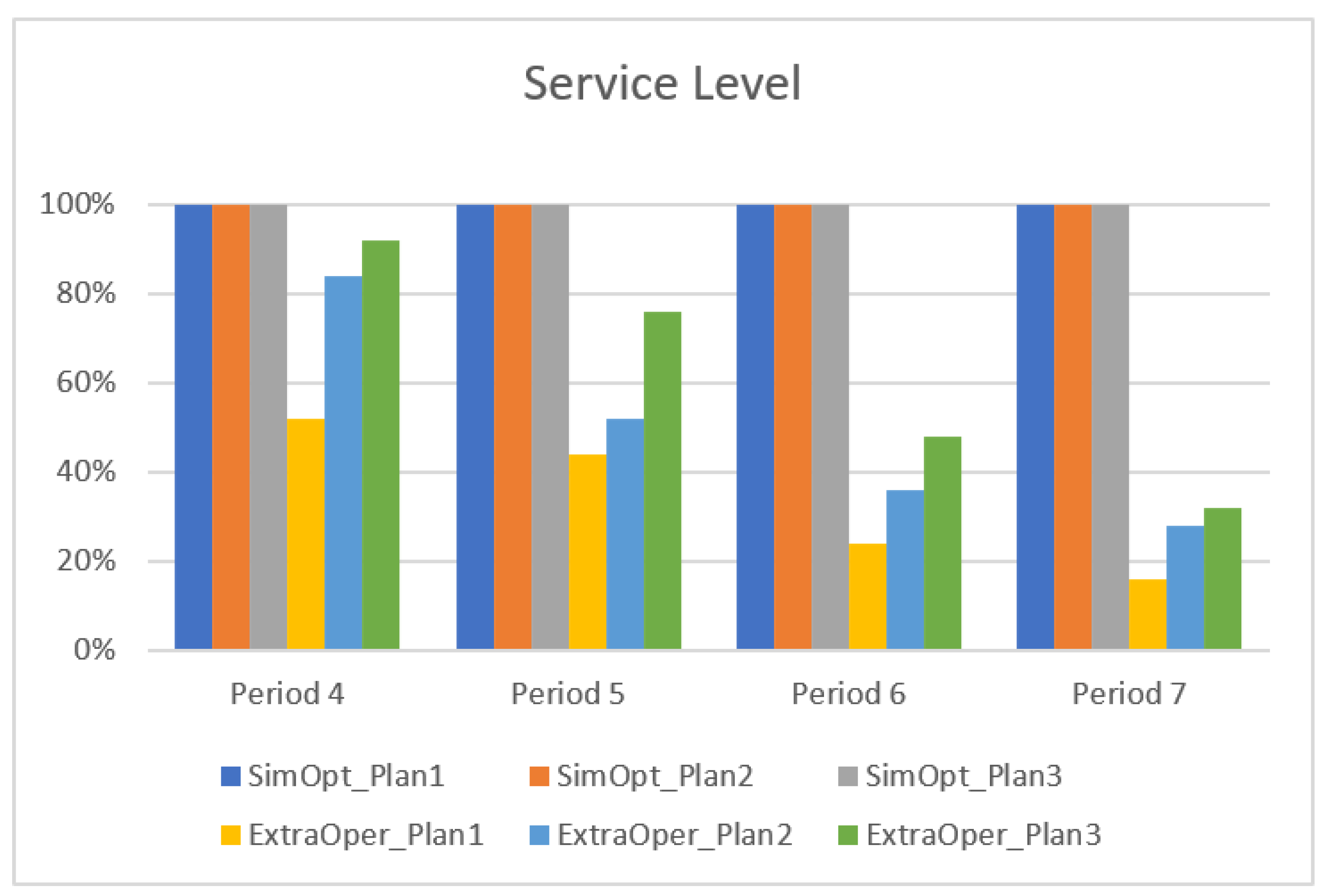
A simulation/optimisation approach was the basis for the development of a mitigation strategy whose performance was compared with a “extra operations” (simulation heuristics) strategy. The developed approach was able to process all biomass for the three initial plans, by replanning the operations, with no need to add extra operations. The costs are naturally higher, and for a fair comparison purpose, a cost penalty for the unprocessed biomass needs to be incorporated.

In summary, the proposed framework seems to adequately address multiple types of disruptions in biomass supply chains, facilitating the assessment and selection of operational plans and the replanning process.

The decision support tool proposed in this work was developed for the forest-to-bioenergy sector, but the performed experiments show its robustness and efficiency, suggesting a possible replication of the methodology to other sectors. Moreover, complementary work should be done to address different types of disruptive events such as uncertainty in breakdowns, machine deterioration, increase in demand and transport delays. Moreover, different forms of biomass and uncertainty on the biomass availability in the piles could be considered, as a way to increase resilience.

It should also be noted that approaches linking planning, monitoring, and control systems with IoT components, still need to be more widely used. In terms of future work, IoT components could be added to the system, providing the basis for a “digital twin” of the supply chain. In fact, providing decision-makers with a steady stream of real-time data will support the creation of more flexible contingency plans, and the design of effective disaster response strategies.

Finally, from the decision maker’s perspective, the design and adoption of broader supply chain resilience metrics could provide planners with insights on how to better manage the risk of disruptions. Extending the current system to explicitly include a multi-objective decision platform would allow the decision-makers to explore trade-off strategies, taking into account the perspectives of the different stakeholders.