


Regional Differences and Convergence of Technical Efficiency in China’s Marine Economy under Carbon Emission Constraints

Abstract
:1. Introduction
2. Literature Review
2.1. Sustainable Development of the Marine Economy
2.2. Efficiency of Marine Economy
3. Research Design
3.1. Model of Measurement of Marine Technical Efficiency and Influencing Factors
3.1.1. Basic Model
3.1.2. Variable Design
- (1)
- Input-output variablesSince Equations (1) and (2) both contain production frontier functions, choosing reasonable input-output variables is significant to measure technical efficiency scientifically. Referring to the existing literature and based on the research objectives of this paper, the following input-output variables are selected:
- ①
- Output variableGross ocean product (Gop): Gross ocean product in the coastal provinces reflects the economic output of the marine economy in each province. To reduce the impact of price on the gross ocean product, this paper takes 2005 as the base period to calculate the actual value of the gross ocean product of each province. The GOP data is from China Marine Statistical Yearbook.
- ②
- Input variables
- Carbon dioxide emission (CO2): The paper adopts a single-output SFA model, so carbon dioxide emission is analyzed as an input variable. Since carbon dioxide emission is not published by each province directly, the carbon dioxide emission data used in each province are derived from the China Emission Accounts and Datasets (CEADs) [37,38,39] which are compiled by several research institutes. Because most scholars have shown that GDP has an obvious positive correlation with carbon emissions, the carbon dioxide emissions of marine industries in each province can be calculated by multiplying the proportion of gross marine product to the gross domestic product by carbon dioxide emissions in the province.
- Labor input (L): It reflects the changes in the number of employees in the process of marine economic development in each province. This paper selects “sea-related employment” as the labor input variable. Data comes from China Marine Statistical Yearbook.
- Capital input (K): Due to the lack of capital input of the marine economy in related provinces in the existing statistical data, it selects the fixed investment in the marine economy of each province as capital input. It is calculated by total investment in fixed assets and the proportion of gross ocean product in the gross domestic product in each province. It also selects 2005 as the base year. The data on total investment in fixed assets comes from China Statistical Yearbook.
- (2)
- Influencing factors variables
- ①
- Industrial structure (Is): Marine-related industries can be divided into the first, second, and third industries. Among them, the marine secondary industry mainly consists of manufacturing and mining sectors, with more carbon emissions than other industries. Therefore, it adopts the proportion of gross ocean product in the secondary industry to gross ocean product as an indicator to measure the industrial structure. It assumes that this indicator has a negative impact on η in each province. GOP in the secondary industry comes from China Marine Statistical Yearbook.
- ②
- Structure of property rights (Prs): In the context of economic restructuring, many state-owned and private enterprises coexist in China’s marine-related industries. Studies have shown that the efficiency of state-owned enterprises is lower than that of private enterprises [40,41]. Therefore, the variable adopted is the proportion of the number of people employed by state-owned enterprises to the total employment in the province at the end of the year. These indicators are from the China Statistical Yearbook and the Statistical Yearbook of each province. It assumes that this proportion has a negative impact on η.
- ③
- Foreign direct investment (FDI): Foreign direct investment has brought about the intensification of the connection between the domestic market and the international market. The increase in Sino-foreign joint ventures, Sino-foreign cooperative operations, and wholly foreign-owned enterprises can increase competition among enterprises, and promote the upgrading of industrial structure and improvement of technological level. As a result, this paper examines the influence of foreign direct investment on the technical efficiency of China’s marine low-carbon economy, assuming that foreign direct investment has a positive impact on η. Data comes from China Statistical Yearbook.
- ④
- Energy structure (Es): Carbon emissions from different energy sources used in the production process are also very different. If the use of carbon-containing energy accounts for a relatively large proportion, the carbon emission will be relatively high. Therefore, it chooses the proportion that coal consumption accounts for total energy consumption as a proxy variable of energy structure. The data on different energy consumption is from China Energy Statistics Yearbook. It assumes that it has a significant negative impact on η.
- ⑤
- Energy price (Ep): In general, high energy prices will increase producers’ costs. Therefore, to reduce costs, producers will heighten energy efficiency as much as possible. It selects purchasing price indicator for raw materials, fuels, and power of producers in each province as a proxy variable for energy price, which comes from China Statistical Yearbook, and the indicator is converted in the base period of 2005. It assumes that this variable has a positive impact on η.
- ⑥
- Technique level (Tec): Under normal circumstances, the research results of scientific research institutions can greatly promote the improvement of the technical level of related industries [42]. The number of scientific papers published by marine scientific research institutions can indicate the status of marine scientific research institutions engaged in research and development within a period. A large number of published scientific papers indicates that the R&D achievements are rich, which can promote the improvement of the technical level of the marine economy and improve efficiency. In this paper, the number of scientific and technological papers of marine scientific research institutions in each province is selected as the proxy variable of technical level, assuming that the variable has a positive impact on η. Data comes from China Marine Statistical Yearbook. Special definition of each variable can be found in Table 1.
3.1.3. Econometric Model
3.2. Kernel Density Estimation
3.3. Stochastic Convergence of Technical Efficiency
3.4. Sample Selection and Data Sources
4. Empirical Results
4.1. Stability Test and Cointegration Test
4.2. Stochastic Convergence of Technical Efficiency
4.3. Dynamic Evolution of Technical Efficiency
4.4. Analysis of Factors Influencing Technical Efficiency of the Marine Economy
4.5. Stochastic Convergence
5. Conclusions
- (1)
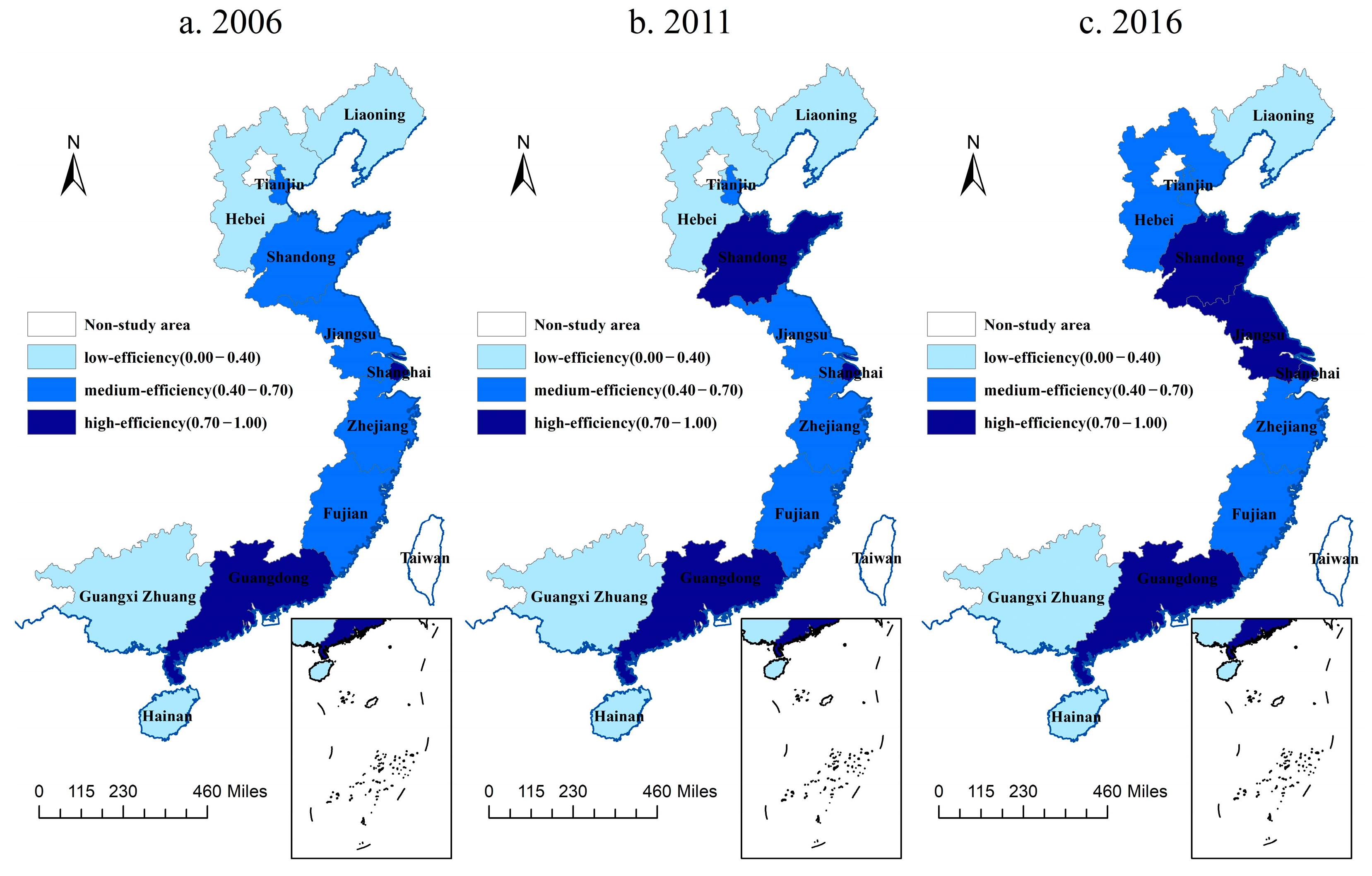
- The technical efficiency of the marine low-carbon economy varies substantially in different regions of China. During the study period, the maximum and minimum annual average values of η are 0.4917 and 0.6037, respectively. The overall η of all provinces and cities is on the rise. Guangdong and Shanghai are in the lead. The technical efficiency of Guangdong has surpassed Shanghai since 2010 and reached 0.9895 in 2016. The marine economic development of Fujian does not match the η. The marine economic development is relatively good, but the η is low. The technical efficiencies of Hainan and Guangxi provinces are relatively low, both below 0.3. The coefficients of variation of the 11 coastal provinces are large. Therefore, the government needs to further increase its emphasis on marine science and technology, and strengthen cooperation within various regions and the entire coastal area to reduce regional gaps and improve coordinated development capabilities.
- (2)
- From 2006 to 2009, the technical efficiency of coastal provinces is generally low, and there is a cluster of η in various regions. As time passed, the 11 provinces and cities began to differentiate gradually, and the technical efficiency of some provinces increased. However, apart from the Yangtze River Delta and the Pan-Pearl River Delta, there is no common development trend in other regions and the entire 11 coastal provinces and cities. In general, the changes in η in coastal provinces have shown a process from concentration to differentiation. The development gap between regions has become larger, and the development speed of each province is different. Based on strengthening cooperation, local governments should continue to strengthen their support for marine economic development and constraints on marine environmental management.
- (3)
- The number of marine scientific papers published and the proportion of the output value of marine secondary industry have a positive effect on η, while the proportion of state-owned enterprise employment, foreign direct investment, producer purchase price index, and coal consumption proportion have a negative impact on η. The influence of property rights structure, industrial structure, and energy consumption structure is more obvious. As a result, the government must continue to promote low-carbon production in the marine economy, actively encourage private capital to invest in marine-related industries, and heighten the development of the marine low-carbon economy through advances in marine science and technology.
Author Contributions
Funding
Institutional Review Board Statement
Informed Consent Statement
Data Availability Statement
Conflicts of Interest
References
- Fernández-Macho, J.; González, P.; Virto, J. An index to assess maritime importance in the European Atlantic economy. Mar. Policy 2016, 64, 72–81. [Google Scholar] [CrossRef]
- Arbolino, R.; De Simone, L.; Carlucci, F.; Yigitcanlar, T.; Ioppolo, G. Towards a sustainable industrial ecology: Implementation of a novel approach in the performance evaluation of Italian regions. J. Clean. Prod. 2018, 178, 220–236. [Google Scholar] [CrossRef]
- Wang, Y.; Wang, N. The role of the marine industry in China’s national economy: An input–output analysis. Mar. Policy 2019, 99, 42–49. [Google Scholar] [CrossRef]
- Friedlingstein, P.; Andrew, R.M.; Rogelj, J.; Peters, G.P.; Canadell, J.G.; Knutti, R.; Luderer, G.; Raupach, M.R.; Schaeffer, M.; van Vuuren, D.P.; et al. Persistent growth of CO2 emissions and implications for reaching climate targets. Nat. Geosci. 2014, 7, 709–715. [Google Scholar] [CrossRef]
- Lin, Y. Coupling analysis of marine ecology and economy: Case study of Shanghai, China. Ocean Coast. Manag. 2020, 195, 105278. [Google Scholar] [CrossRef]
- Fu, X.; Kong, W.; Jiang, Q.; Zhang, M. China’s marine economy growth and marine environment pollution: An empirical test based on generalized impulse response function. China Fish. Econ. 2016, 6, 83–88. [Google Scholar]
- Kang, S.; Rui-Rui, C.; Jing-Feng, C. Co-evolution simulation research of marine economy sustainalble development path. China Popul. Resour. Environ. 2014, 11, 395–398. [Google Scholar]
- Ren, W.; Wang, Q.; Ji, J. Research on China’s marine economic growth pattern: An empirical analysis of China’s eleven coastal regions. Mar. Policy 2018, 87, 158–166. [Google Scholar] [CrossRef]
- Ren, W.; Ji, J. How do environmental regulation and technological innovation affect the sustainable development of marine economy: New evidence from China’s coastal provinces and cities. Mar. Policy 2021, 128, 104468. [Google Scholar] [CrossRef]
- Ye, F.; Quan, Y.; He, Y.; Lin, X. The impact of government preferences and environmental regulations on green development of China’s marine economy. Environ. Impact Assess. Rev. 2021, 87, 106522. [Google Scholar] [CrossRef]
- Bennett, N.J. Navigating a just and inclusive path towards sustainable oceans. Mar. Policy 2018, 97, 139–146. [Google Scholar] [CrossRef]
- Islam, M.M.; Shamsuddoha, M. Coastal and marine conservation strategy for Bangladesh in the context of achieving blue growth and sustainable development goals (SDGs). Environ. Sci. Policy 2018, 87, 45–54. [Google Scholar] [CrossRef]
- Liu, W.; Li, F.; Che, K.; Umole, C.; Jia, Z.; Li, Q. Study on the comprehensive evaluation of low carbon city based on PSR model and normalized index transformation. E3S Web Conf. 2020, 194, 05050. [Google Scholar] [CrossRef]
- Shi, B.; Yang, H.; Wang, J.; Zhao, J. City green economy evaluation: Empirical evidence from 15 sub-provincial cities in China. Sustainability 2016, 8, 551. [Google Scholar] [CrossRef]
- Wang, X.E.; Wang, S.; Wang, X.; Li, W.; Song, J.; Duan, H.; Wang, S. The assessment of carbon performance under the region-sector perspective based on the nonparametric estimation: A case study of the northern province in China. Sustainability 2019, 11, 6031. [Google Scholar] [CrossRef]
- Yang, X.; Li, R. Investigating low-carbon city: Empirical study of Shanghai. Sustainability 2018, 10, 1054. [Google Scholar] [CrossRef]
- Keivani, E.; Abbaspour, M.; Abedi, Z.; Ahmadian, M. Promotion of Low-Carbon Economy through Efficiency Analysis: A Case Study of a Petrochemical Plant. Int. J. Environ. Res. 2020, 15, 45–55. [Google Scholar] [CrossRef]
- Li, W.; Bao, L.; Wang, L.; Li, Y.; Mai, X. Comparative evaluation of global low-carbon urban transport. Technol. Forecast. Soc. Chang. 2019, 143, 14–26. [Google Scholar] [CrossRef]
- Meng, M.; Fu, Y.; Wang, T.; Jing, K. Analysis of low-carbon economy efficiency of Chinese industrial sectors based on a RAM model with undesirable outputs. Sustainability 2017, 9, 451. [Google Scholar] [CrossRef]
- Ren, W.; Ji, J.; Chen, L.; Zhang, Y. Evaluation of China’s marine economic efficiency under environmental constraints—An empirical analysis of China’s eleven coastal regions. J. Clean. Prod. 2018, 184, 806–814. [Google Scholar] [CrossRef]
- Ding, L.; Yang, Y.; Wang, L.; Calin, A.C. Cross Efficiency Assessment of China’s marine economy under environmental governance. Ocean Coast. Manag. 2020, 193, 105245. [Google Scholar] [CrossRef]
- Zheng, H.; Zhang, L.; Zhao, X. How does environmental regulation moderate the relationship between foreign direct investment and marine green economy efficiency: An empirical evidence from China’s coastal areas. Ocean Coast. Manag. 2022, 219, 106077. [Google Scholar] [CrossRef]
- Proskuryakova, L.; Kovalev, A. Measuring energy efficiency: Is energy intensity a good evidence base? Appl. Energy 2015, 138, 450–459. [Google Scholar] [CrossRef]
- Wang, Z.; Yuan, F.; Han, Z. Convergence and management policy of marine resource utilization efficiency in coastal regions of China. Ocean Coast. Manag. 2019, 178, 104854. [Google Scholar] [CrossRef]
- Zhang, Y.; Wang, W.; Liang, L.; Wang, D.; Cui, X.; Wei, W. Spatial-temporal pattern evolution and driving factors of China’s energy efficiency under low-carbon economy. Sci. Total Environ. 2020, 739, 140197. [Google Scholar] [CrossRef]
- Laso, J.; Vázquez-Rowe, I.; Margallo, M.; Irabien, Á.; Aldaco, R. Revisiting the LCA+DEA method in fishing fleets. How should we be measuring efficiency? Mar. Policy 2018, 91, 34–40. [Google Scholar] [CrossRef]
- Li, G.; Zhou, Y.; Liu, F.; Wang, T. Regional differences of manufacturing green development efficiency considering undesirable outputs in the Yangtze River Economic Belt based on super-SBM and WSR system methodology. Front. Environ. Sci. 2021, 8, 631911. [Google Scholar] [CrossRef]
- Van Nguyen, Q.; Pascoe, S.; Coglan, L. Implications of regional economic conditions on the distribution of technical efficiency: Examples from coastal trawl vessels in Vietnam. Mar. Policy 2019, 102, 51–60. [Google Scholar] [CrossRef]
- Li, G.; Zhou, Y.; Liu, F.; Tian, A.R. Regional difference and convergence analysis of marine science and technology innovation efficiency in China. Ocean Coast. Manag. 2021, 205, 105581. [Google Scholar] [CrossRef]
- Li, S.J.; Fan, C. Analysis and comparison of stochastic frontier analysis and data envelopment analysis method. Stat. Decis. 2009, 7, 25–27. [Google Scholar]
- Kontodimopoulos, N.; Papathanasiou, N.D.; Flokou, A.; Tountas, Y.; Niakas, D. The impact of non-discretionary factors on DEA and SFA technical efficiency differences. J. Med. Syst. 2011, 35, 981–989. [Google Scholar] [CrossRef]
- Zhu, C.L.; Yue, H.Z.; Shi, P. Studies on China’s economic growth efficiency under the environmental constraints. J. Quant. Tech. Econ. 2011, 5, 3–20. [Google Scholar]
- Niavis, S.; Vlontzos, G. Seeking for Convergence in the agricultural sector performance under the changes of uruguay round and 1992 CAP reform. Sustainability 2019, 11, 4006. [Google Scholar] [CrossRef]
- Yang, W.; Shi, J.; Qiao, H.; Shao, Y.; Wang, S. Regional technical efficiency of Chinese iron and steel industry based on bootstrap network data envelopment analysis. Socio-Econ. Plan. Sci. 2017, 57, 14–24. [Google Scholar] [CrossRef]
- Farrell, M.J. The measurement of productive efficiency. J. R. Stat. Soc. 1957, 120, 253–281. [Google Scholar] [CrossRef]
- Battese, G.E.; Coelli, T.J. A model or technical inefficiency effects in a stochastic production frontier for panel data. Empir. Econ. 1995, 20, 325–332. [Google Scholar] [CrossRef]
- Shan, Y.; Guan, D.; Zheng, H.; Ou, J.; Li, Y.; Meng, J.; Mi, Z.; Liu, Z.; Zhang, Q. Data descriptor: China CO2 emission accounts 1997–2015. Sci. Data 2018, 5, 170201. [Google Scholar] [CrossRef]
- Shan, Y.; Huang, Q.; Guan, D.; Hubacek, K. China CO2 emission accounts 2016–2017. Sci. Data 2020, 7, 54. [Google Scholar] [CrossRef]
- Shan, Y.; Liu, J.; Liu, Z.; Xu, X.; Shao, S.; Wang, P.; Guan, D. New provincial CO2 emission inventories in China based on apparent energy consumption data and updated emission factors. Appl. Energy 2016, 184, 742–750. [Google Scholar] [CrossRef]
- Arocena, P.; Oliveros, D. The efficiency of state-owned and privatized firms: Does ownership make a difference? Int. J. Prod. Econ. 2012, 140, 457–465. [Google Scholar] [CrossRef]
- Lu, T.; Liu, X.X. The Gaizhi models and Gaizhi performance in Chinese transition-based on empirical analysis on the firm survey data. Econ. Res. J. 2005, 6, 94–103. [Google Scholar]
- Xu, X.F.; Wei, Z.F.; Ji, Q.; Wang, C.L.; Gao, G.W. Global renewable energy development: Influencing factors, trend predictions and countermeasures. Resour. Policy 2019, 63, 101470. [Google Scholar] [CrossRef]
- Onghena, E.; Meersman, H.; Van de Voorde, E. A translog cost function of the integrated air freight business: The case of FedEx and UPS. Transp. Res. Part A Policy Pract. 2014, 62, 81–97. [Google Scholar] [CrossRef]
- Carlino, G.A.; Mills, L.O. Are U.S. regional incomes converging?: A time series analysis. J. Monet. Econ. 1993, 32, 335–346. [Google Scholar] [CrossRef]
- Evans, P.; Karras, G. Convergence revisited. J. Monet. Econ. 1966, 37, 249–265. [Google Scholar] [CrossRef]
- Luo, Y.; Lu, Z.; Long, X. Heterogeneous effects of endogenous and foreign innovation on CO2 emissions stochastic convergence across China. Energy Econ. 2020, 91, 104893. [Google Scholar] [CrossRef]


| Variables | Units | Hyp. | Sym. | Proxy Variables |
|---|---|---|---|---|
| Output | 10,000 RMB | - | Gop | Gross ocean product, 2005 as the basic year |
| Carbon dioxide emissions | 10,000 tons | - | CO2 | Carbon dioxide emission in the marine economy |
| Labor input | 10,000 people | - | L | Sea-related employment |
| Capital input | 10,000 RMB | - | K | Fixed investment in the marine economy, 2005 as the basic year |
| Industrial structure | - | negative | Is | The output value of the marine secondary industry/GOP |
| Structure of property rights | - | negative | Prs | People employed by state-owned enterprises/Total employment |
| Foreign direct investment | 100,000,000 USD | positive | Fdi | Foreign direct investment |
| Energy structure | - | negative | Es | Coal consumption/Total energy consumption |
| Energy price | - | positive | Ep | Purchasing price indicator for raw materials, fuels, and power of producers, 2005 as the basic year |
| Technique level | papers | positive | Tec | Number of scientific papers published by marine scientific research institutions |
| Variables | Maximum | Minimum | Mean | Standard Deviation |
|---|---|---|---|---|
| Gop | 62,713,393.23 | 3,007,000.00 | 22,908,260.97 | 15,729,348.43 |
| CO2 | 21,411.22 | 427.22 | 5448.86 | 4288.09 |
| L | 868.50 | 81.50 | 305.04 | 210.13 |
| K | 88,204,902.50 | 1,239,446.77 | 18,860,537.44 | 15,516,497.74 |
| Is | 0.68 | 0.19 | 0.44 | 0.10 |
| Prs | 0.75 | 0.16 | 0.40 | 0.16 |
| Fdi | 357.60 | 4.47 | 117.56 | 88.95 |
| Es | 0.80 | 0.26 | 0.54 | 0.14 |
| Ep | 143.67 | 95.62 | 116.28 | 10.79 |
| Tec | 3072.00 | 11.00 | 724.94 | 638.80 |
| Variables | Original Value | First-Order Difference | ||
|---|---|---|---|---|
| T-Statistic | p-Value | T-Statistic | p-Value | |
| lnGop | 16.6852 | 0.7805 | 56.1110 | 0.0001 |
| lnCO2 | 30.7089 | 0.1022 | 77.4750 | 0.0000 |
| lnL | 110.440 | 0.0000 | 175.527 | 0.0000 |
| lnK | 8.76834 | 0.9945 | 78.0923 | 0.0000 |
| [lnCO2]2 | 29.5350 | 0.1302 | 77.0286 | 0.0000 |
| [lnL]2 | 108.457 | 0.0000 | 173.605 | 0.0000 |
| [lnK]2 | 7.68797 | 0.9979 | 80.4224 | 0.0000 |
| [lnCO2] × [lnL] | 31.5872 | 0.0847 | 44.2881 | 0.0033 |
| [lnCO2] × [lnK] | 26.6369 | 0.2253 | 79.8509 | 0.0000 |
| [lnL] × [lnK] | 17.1298 | 0.7562 | 59.2864 | 0.0000 |
| Is | 13.6180 | 0.9145 | 57.2918 | 0.0001 |
| Prs | 6.11158 | 0.9997 | 43.2067 | 0.0045 |
| Fdi | 30.7492 | 0.1014 | 78.8859 | 0.0000 |
| Es | 17.3342 | 0.7447 | 56.2237 | 0.0001 |
| Ep | 30.9632 | 0.0969 | 46.8718 | 0.0015 |
| Tec | 26.9372 | 0.2136 | 77.1782 | 0.0000 |
| Var. | Par. | Statistical Magnitude | Var. | Par. | Statistical Magnitude | ||
|---|---|---|---|---|---|---|---|
| Estimated Value | T Statistics | Estimated Value | T Statistics | ||||
| Cons | β0 | −21.169 *** | −11.117 | Cons | ξ0 | 0.210 | 1.272 |
| lnCO2 | β1 | 0.744 | 1.629 | Is | ξ1 | −1.318 *** | −8.155 |
| lnL | β2 | −0.753 | −1.151 | Prs | ξ2 | 0.783 *** | 3.885 |
| lnK | β3 | 4.315 *** | 16.294 | Fdi | ξ3 | 0.0002 | −1.707 |
| [lnCO2]2 | β4 | 0.424 *** | 8.214 | Es | ξ4 | 0.871 *** | 3.938 |
| [lnL]2 | β5 | 0.028 | 0.999 | Ep | ξ5 | 0.006 *** | 3.933 |
| [lnK]2 | β6 | −0.236 *** | −17.328 | Tec | ξ6 | −0.001 *** | −8.892 |
| [lnCO2] × [lnL] | β7 | −1.236 *** | −8.093 | σ2 | - | 0.021 *** | 7.880 |
| [lnCO2] × [lnK] | β8 | −0.043 | −0.775 | γ | - | 0.988 *** | 77.947 |
| [lnL] × [lnK] | β9 | 0.682 *** | 8.523 | - | - | - | - |
| 2006 | 2007 | 2008 | 2009 | 2010 | 2011 | 2012 | 2013 | 2014 | 2015 | 2016 | Mean | Region | |
|---|---|---|---|---|---|---|---|---|---|---|---|---|---|
| Tianjin | 0.5068 | 0.5118 | 0.5404 | 0.5511 | 0.5704 | 0.5585 | 0.6094 | 0.6489 | 0.7391 | 0.9395 | 0.6045 | 0.6164 | Bohai Rim |
| Hebei | 0.2831 | 0.2836 | 0.3007 | 0.3217 | 0.3211 | 0.3132 | 0.3257 | 0.3408 | 0.3994 | 0.4010 | 0.4304 | 0.3383 | Bohai Rim |
| Liaoning | 0.3147 | 0.3289 | 0.3400 | 0.3310 | 0.3431 | 0.3791 | 0.3678 | 0.3845 | 0.3816 | 0.3378 | 0.3457 | 0.3504 | Bohai Rim |
| Shanghai | 0.9764 | 0.9903 | 0.9557 | 0.8600 | 0.8559 | 0.8229 | 0.8170 | 0.7799 | 0.8198 | 0.8174 | 0.8634 | 0.8690 | Yangtze River Delta |
| Jiangsu | 0.4819 | 0.5264 | 0.5226 | 0.5618 | 0.6003 | 0.5993 | 0.6314 | 0.6387 | 0.7173 | 0.7601 | 0.7825 | 0.6202 | Yangtze River Delta |
| Zhejiang | 0.4350 | 0.4466 | 0.4796 | 0.5136 | 0.5169 | 0.5458 | 0.5232 | 0.5024 | 0.4714 | 0.4850 | 0.4933 | 0.4921 | Yangtze River Delta |
| Fujian | 0.4062 | 0.4104 | 0.4102 | 0.4324 | 0.4196 | 0.4362 | 0.3917 | 0.3872 | 0.4438 | 0.5117 | 0.5400 | 0.4354 | Pan-Pearl River Delta |
| Shandong | 0.6318 | 0.6830 | 0.7135 | 0.6882 | 0.7312 | 0.7503 | 0.7665 | 0.8149 | 0.8683 | 0.9001 | 0.9171 | 0.7696 | Bohai Rim |
| Guangdong | 0.7718 | 0.6836 | 0.8301 | 0.8322 | 0.9282 | 0.9798 | 0.9876 | 0.9328 | 0.9880 | 0.9806 | 0.9895 | 0.9004 | Pan-Pearl River Delta |
| Guangxi | 0.3308 | 0.2807 | 0.2724 | 0.2457 | 0.2568 | 0.2508 | 0.2657 | 0.2829 | 0.3000 | 0.3204 | 0.3366 | 0.2857 | Pan-Pearl River Delta |
| Hainan | 0.2704 | 0.2957 | 0.2758 | 0.2270 | 0.2104 | 0.2035 | 0.1994 | 0.2056 | 0.1893 | 0.1872 | 0.2013 | 0.2242 | Pan-Pearl River Delta |
| Mean | 0.4917 | 0.4946 | 0.5128 | 0.5059 | 0.5231 | 0.5308 | 0.5351 | 0.5381 | 0.5744 | 0.6037 | 0.5913 | - | - |
| Maximum | 0.9764 | 0.9903 | 0.9557 | 0.8600 | 0.9282 | 0.9798 | 0.9876 | 0.9328 | 0.9880 | 0.9806 | 0.9895 | - | - |
| Minimum | 0.2704 | 0.2807 | 0.2724 | 0.2270 | 0.2104 | 0.2035 | 0.1994 | 0.2056 | 0.1893 | 0.1872 | 0.2013 | - | - |
| Regions | IPS W-Stat | p-Value | ADF-Fisher Chi-Square | p-Value | PP-Fisher Chi-Square | p-Value |
|---|---|---|---|---|---|---|
| 11 coastal provinces and cities | −0.110 | 0.456 | 26.274 | 0.240 | 12.232 | 0.952 |
| Three regions | −0.319 | 0.375 | 7.958 | 0.241 | 4.505 | 0.609 |
| Yangtze River Delta | −1.691 | 0.046 | 13.075 | 0.042 | 13.454 | 0.036 |
| Pan-Pearl River Delta | −1.440 | 0.075 | 15.507 | 0.050 | 3.464 | 0.902 |
| Bohai Rim | 1.249 | 0.894 | 4.833 | 0.775 | 4.597 | 0.800 |
Disclaimer/Publisher’s Note: The statements, opinions and data contained in all publications are solely those of the individual author(s) and contributor(s) and not of MDPI and/or the editor(s). MDPI and/or the editor(s) disclaim responsibility for any injury to people or property resulting from any ideas, methods, instructions or products referred to in the content. |
© 2023 by the authors. Licensee MDPI, Basel, Switzerland. This article is an open access article distributed under the terms and conditions of the Creative Commons Attribution (CC BY) license (https://creativecommons.org/licenses/by/4.0/).
Share and Cite
Li, G.; Wang, J.; Liu, F.; Wang, T.; Zhou, Y.; Tian, A. Regional Differences and Convergence of Technical Efficiency in China’s Marine Economy under Carbon Emission Constraints. Sustainability 2023, 15, 7632. https://doi.org/10.3390/su15097632
Li G, Wang J, Liu F, Wang T, Zhou Y, Tian A. Regional Differences and Convergence of Technical Efficiency in China’s Marine Economy under Carbon Emission Constraints. Sustainability. 2023; 15(9):7632. https://doi.org/10.3390/su15097632
Chicago/Turabian StyleLi, Gen, Jingwen Wang, Fan Liu, Tao Wang, Ying Zhou, and Airui Tian. 2023. "Regional Differences and Convergence of Technical Efficiency in China’s Marine Economy under Carbon Emission Constraints" Sustainability 15, no. 9: 7632. https://doi.org/10.3390/su15097632
APA StyleLi, G., Wang, J., Liu, F., Wang, T., Zhou, Y., & Tian, A. (2023). Regional Differences and Convergence of Technical Efficiency in China’s Marine Economy under Carbon Emission Constraints. Sustainability, 15(9), 7632. https://doi.org/10.3390/su15097632