Poverty and Gender: Determinants of Female- and Male-Headed Households with Children in Poverty in the USA, 2019

Abstract

Attaining economic parity and reducing poverty between the genders are critical steps toward attaining the United Nations’ Sustainable Development Goals. Despite progress, women in the US still earn USD 0.83 for every USD 1.00 that a man earns. With rising shares of single/female-headed households with children in American society in recent years, such gaps in earnings exacerbate the misery of children living in such households. In 2019, female-headed households with children had poverty rates almost twice (36.5%) that of single/male-headed families (16.3%). This paper uses five-year American Community Survey estimates from the National Historical Geographic Information System to empirically examine the spatial distribution and determinants of female-versus-male-headed households with children living in poverty in the counties of the USA. Lower levels of educational attainment are associated with higher levels of poverty for both genders. A bachelor’s degree in education is associated with higher poverty for female-headed households, whereas majoring in business, sciences, engineering, and arts/humanities is associated with lower poverty for male-headed households. Service-sector occupations inherently contribute to higher poverty for both groups. Over-representation in management/professional and natural-resources, construction, and maintenance-type occupations works well for male-headed households, whereas management/professional, sales/office, and service-based occupations associate with higher poverty for female-headed households—pointing toward the “working poor”—comprising largely of the active female labor force in the new economy. Full- and part-time work status alleviates poverty for female-headed households, whereas part-time work is associated with higher poverty for males.

1. Introduction

On 8 March 2023, the United Nations’ Chief Guterres made international news when he noted that it would take another 300 years to attain gender equality in the world [1]. Despite this harsh reality for women all around the world, this statement should be accepted with humility, as disproportionate levels of income inequality and gender poverty have remained major concerns well into the twenty-first century. While significant economic growth and progress have been made all over the world, income inequality and a lack of upward mobility have remained important topics of academic scholarship for quite some time. Even with visible economic growth and progress since the recession of 2007–2009, the gaps between the rich and the poor have continued in the US, and these gaps have become more exacerbated for women compared to men in all age groups and far worse for women of color compared to men of the same races/ethnicities.

Income inequality is unavoidable in any society, but too much inequality can permanently damage the fabric of a social system. A society where the rich become richer and the poor become poorer can have serious consequences for the overall health and wellbeing of its population [2,3,4]. The negative consequences of such gaps manifest through numerous social, economic, and cultural break-ups in a society, and inadvertently, women are impacted by these much worse compared to men across all racial/ethnic groups, including increased rates of divorce, a rise in single-parent households, negligence of children involved in broken marriages, and the like. Even now, women continue to earn only USD 0.83 for every USD 1.00 that a man earns [5]. Based on the US Census Bureau, there seems to be a strong “motherhood penalty” [1]. Despite reasonable success in educational and occupational attainment, women have still been unable to fully translate their human capital skills and credentials into economic success [6,7,8]. Globally, never-married women are the fastest-growing cohort in the labor market, yet their median earning is 92.1% of what never-married men make, and this gap has increased during the last decade, when they earned 95.8% of what men earned [1]. In the USA, single women with children have a median family wealth of USD 7000 compared to USD 59,000 for single men with children; these statistics for single women versus single men without children are USD 57,000 and USD 65,000, respectively [1,9]. However, whether these earnings and wealth gaps between single male-headed households and single female-headed households translate differently in terms of poverty levels is still unknown. This paper specifically focuses on this aspect of contemporary poverty and inequality across the genders—an everyday truth of American society where the share of single/divorced (Since the data pertains to female-headed households, with or without children (no-spouse present), for this analysis I am assuming that these might be the divorced, single-mom/single-dad cases, and hence I use single/divorced in the text for simplicity) women and female-headed households has been increasing, with much greater financial burdens felt by them and especially by those who have children.

This paper, thus, examines the spatial patterns of single-male-headed households with children and single-female-headed households with children living in poverty in the counties of the USA. Further, it also attempts to empirically explain the varying levels of poverty for these groups by exploring their association with detailed categories of select explanatory variables pertaining to educational and occupational attainments and their work status—all of which are critical toward improving one’s earnings potential. This paper uses data from the five-year (2015–2019) American Community Survey (ACS) estimates available from the National Historical Geographic Information System (NHGIS) [10]. In addressing the above purposes, I use county as the scale of analysis, whereas three types of dependent variables include: (1) female-headed households with children living in poverty; (2) female-headed households without children living in poverty; and (3) male-headed households with children living in poverty. This research finds that higher levels of poverty among single female-headed households correlate strongly with the black population in the country. Additionally, while lower educational attainments associate with higher poverty for both genders, female-headed households have disadvantages if they graduate with education majors whereas majors in science, engineering, business, and arts/humanities associate with lower poverty among male-headed households. An interesting finding of this research points toward the “working poor”—largely the female-headed households (with and without children), comprising an active labor force in the new economy, who suffer the greatest risks of living in poverty.

2. Background Context

2.1. A Brief Overview of Gendered Work and Wage Gaps

Throughout the world, extreme levels of wealth and income concentration have strengthened the economic and political power of a few individuals—largely males, comprising the topmost segment of society [9]. Globally and within the US, women are underrepresented in the highest-paid and best-quality positions [9,11]. Women are overrepresented in service sectors and other occupations such as restaurant services, retail, tourism, front-desk clericals, care activities, and hospitality that are traditionally associated with lower wages [6,12]. The enormous amount of time spent on unpaid activities could have been utilized toward productive and income-generating livelihoods, which could have contributed to their economic wellbeing [13,14]. Even now, based on the U.S. Department of Labor and Fortune, female-dominated occupations such as childcare and restaurant service work continue to occupy the lower rungs of the U.S. wage ladder, and women make up 63% of total workers earning the federal minimum wage—a wage rate stuck at USD 7.25 since 2009 [15]. In 2016, women still represented only 5% of CEOs at Fortune 500 firms, whereas CEOs’ average take-home salary was USD 13.1 million [15,16].

Regarding gender equality, the United Nations indicated that in order to achieve gender equality and parity, women must be included in technology and innovation industries such that the United Nations’ Sustainable Development Goals (UN-SDGs) can be achieved—the only blueprint toward creating a just and equitable future by 2030 [17]. It is expected that by mid-century, almost 75% of all jobs will be related to STEM (science, technology, engineering, or math) disciplines, yet women comprise only 30% of the workforce in the world’s 20 largest global tech companies [17]. Within the US, even though women comprise almost half of the country’s workforce, men comprise an overwhelming majority of the top earners. Women hold only 27% of the top 10% of income-earners, 17% of the top 1%, and only 11% of the top 0.1% [11,12]. An analysis of the topmost earners in the US labor force suggests that the share of women in the top 10% earners has increased from about 5% in 1962 to 27.5% in 2014; these figures for the top 1% earners changed from 3% (1962) to 16.5% (2014), and those in the topmost 0.1% changed from 2% (1962) to 11% (2014) only [18]. Such disparities in income/wealth and an overwhelming control of the politically and economically elite top 1% genre are not only confined to the US; instead, they exist all over the world, including several developing economies. Based on a survey conducted during 2010–2014 by the National Bureau of Economic Research and the London School of Economics, in the eight richest/highest-income countries of the world, males comprised the largest shares of the top-paying positions; the same survey also concluded that within the US, in 2012, women comprised only 14–22% of the top 1% earners [19].

Concerning wage gaps, the Economic Policy Institute, the Institute for Women’s Policy Research, and other scholars suggest that in 2016, women working full-time still earned an average of 81 cents for every dollar that a man earned, and these gaps were much wider when part-time workers were included in the sample [20]. These gaps are wider for racial/ethnic groups and for women of color, with the largest pay gaps between men and women of white and Asian groups [21]. This occurs not because Latina and black women have made more progress toward equity; instead, this occurs because the average pay for men in these groups is far below those of whites and Asians, even in 2020 [21]. Further, women generally end up doing a considerably higher amount of unpaid work—from housekeeping to caring for children and the elderly, cooking, cleaning, and everything else, voluntarily or involuntarily, that needs to be carried out to efficiently manage their homes and their household finances [6,7,8,13,14,22]. Recent research has shown that women working in professional/management types of jobs tend to earn a better income [17]. Based on the U.S. Census Bureau (2020), the largest pay gaps between males and females occur in management positions, with men making an average of USD 88,000 in 2016 as against only USD 55,000 for women; the smallest gaps appeared in construction—an industry perceived as masculine, with women comprising only 9% of its total labor force. According to the Institute for Policy Studies’s analysis of World Bank and World Development Indicators, even though the gendered wage gaps in the USA are quite large, they are not the worst, as there are numerous other countries where women do far worse. For example, among the OECD group of higher-income countries, the gap is the highest in South Korea, with men earning 37% more than women; Luxembourg, in contrast, has the narrowest gap, with men making only 3.4% more than women. The gender gaps in OECD countries are smaller because a good proportion of workers are covered by collective bargaining (i.e., union) agreements [15,17].

Based on the International Labor Organization’s (ILO) analysis of data from 21 countries, using data for at least one year from 2013 to 2015, the two countries with the highest imbalance were the West Bank and Gaza, with men devoting only 16% of their time on unpaid domestic and caregiving activities; in contrast, Belgium had the fairest distribution, with men spending 63% of their time on these activities, and they ranked at the top [23,24,25]. While the ILO agrees that more work is needed to develop more accurate global gender gap analyses, in reality, the availability and accessibility of good-quality data have remained a problem for a long time in the majority of the world, and this has dissuaded researchers from engaging in quality and timely research on gender gap analyses. In addition, The Washington Center Report and other scholars suggest that despite numerous policies proposed by the Think Tanks, their approval by Congress, and on-the-ground implementation and abidance, contemporary capitalism is quite challenging [5,26].

2.2. A Factual Overview of Gender Gaps in Poverty

The US, despite being one of the richest economies in the world, still has a significant share of its population living below the poverty line. Though the official poverty rate in 2020 was 11.4%—1% higher than its 2019 level, what is surprising is that this rise in poverty level occurred for the first time after consecutive annual declines during the last five years. About 37.2 million people lived in poverty in 2020—an uptick of 3.3 million since 2019 [21].

When evaluating the long-term change in poverty for the overall population in the US, the Census 2020 income and poverty report indicates that while the statistics changed from 40 million (23.5%) in 1959 to 34 million (10.5%) in 2019, the poverty gap between the genders had indeed widened during these 50–60 years. In 2016, almost 13.4% of adult women (18–64 years), which is about 13.4 million, lived in poverty compared to 9.7% of adult men (9.4 million); in 1968, these statistics were 10.8% (6.1 million) for women and 7.2% for men (3.7 million)—indicating a steep rise for women living in poverty. The poverty rates for females and males in 18–64 years were 10.8% and 8.1%, respectively, in 2019; these figures were 14.5% and 14.4% for children ≤18 years, and 10.3% versus 7.2% for ≥65 years—confirming disadvantage for females across all ages and much worse among the oldest.

Based on reports and figures compiled by the US Census Bureau 2019 and 2020 Annual Social and Economic Supplements (CPS ASEC), the poverty rates between males, females, and married families are significantly different. The poverty rates for married couples as well as female-headed and male-headed households in 2019 were 4.0%, 22.2%, and 11.5%, respectively—indicating the benefits of being in married status and the significantly higher poverty rates for female-headed households [27]. These figures for married couples, female-headed households, and male-headed households when children below the age of 18 lived together were 6.4%, 36.5%, and 16.3%, respectively [27]. According to the National Women’s Law Center, these figures were not much different in 2016, with a poverty rate of 35.6% for single-women headed households with children—more than twice the 17.3% for single-men headed households with children. Based on the Census 2020 report, however, poverty rates also increased for married-coupled families during 2019–2020, from 4% (2019) to 4.7% (2020); these statistics for families with a female head were significantly high—22.2% in 2019, which increased to 23.4% in 2020; the figures for male-headed families during 2019 and 2020 were at about 11.4%, far below female-headed families. Such gaps in poverty rates among families, especially because of their female-versus-male-headed status, can have severe negative impacts, especially when children are involved. Given that most often women are the caretakers of children involved in broken/divorced households, and/or if a woman decides to have children regardless of marriage/partner, they end up suffering from the “motherhood penalty”.

Such exacerbated rates of poverty and unequitable earnings between the genders also have severe implications for their wealth accumulation, retirement savings, and other health insecurities. In the US, men have three times more retirement savings funds compared to women, and when one adds up different types of savings, the gap widens further [28]. Based on the statistics provided by Collinson, the CEO of Transamerica Center for Retirement Studies, in 2017, American women held a median retirement savings of USD 42,000 compared to USD 123,000 for men; the figures for less than USD 10,000 in retirement were 21% for women versus 12% for men. Thus, lifelong gender pay gap translates into old-age insecurities and ailments since the pension plan and Social Security payouts are based partly on their past earnings, and given their old age, a large share of women are physically incapable of contributing toward their finances—which forces them into higher poverty.

2.3. Origin of Gender Inequality and Theoretical Conceptualization

Post-Fordism has been associated with the beginning of the most severe forms of inequality in the USA. While the economic restructuring in the American Manufacturing Belt (AMB) benefitted the Southeastern and Western regions of the USA, it also triggered varied levels of socioeconomic inequalities among different population groups and communities of color, furthering the divide between the richest and the poorest segments over time [3,29,30,31,32,33]. The post-Fordist processes were likened to the decline of middle-class jobs, along with the bifurcation between high-paying jobs that required considerable investment in education and human capital skills versus low-end jobs that required fewer-to-no skills [33,34,35,36,37,38,39]. Given a relatively higher share of women, immigrants, and minorities possessing lower levels of skills and education, they ended up experiencing disproportionate shares of discrimination in the labor market that aggravated already existing inequalities and poverty [40,41,42,43]. The new economy demanded newer, flexible skills, which were accessible to the upper-middle and wealthier segments of society, and those with money, time, and enthusiasm were able to upgrade their skills to fit in and reap the largest margins of the benefits [44,45,46]. However, given the overburdened status of women largely in low-wage paid activities, pulling out time for skill development was difficult. These led to the cyclic reproduction of gendered gaps in earnings. Since the restructuring of the 1970s, several states in the USA have also undergone severe cuts in state-supported welfare-activities, which have had adverse consequences for the poor, minorities, and women, including female-headed households with children [33,34,35,37,39,47].

Finally, in their scholarly endeavors to explain the under- and over-representation of women in low-wage occupations—the crux of earnings gaps and poverty—scholars have used a variety of theoretical lenses. These include Becker’s (1994) Human Capital Theory (HCT), which likens the demand and supply aspects of labor with their over-/under-representation, and the Neoclassical Economic Theory (NET), which attributes pure economic incentives as the driving force in picking up jobs/occupations [22,48]. Both of these theories, however, ignore the complex ways in which the demographic, socio-economic, historical, and cultural contexts of a person’s upbringing impact his/her acquisition of human capital skills that might affect his/her occupational choices. Anne Bonds (2013) and other Feminist Political Ecology (FPE) theorists questioned such simplistic/binary perspectives provided by the HCT and the NET since these masked the complex processes of feminization (and racialization) of economic practices in the contemporary world [49]. The Labor Market Segmentation Theory (LMST) rejects the binary/linear connection between gendered labor market outcomes and their educational skills; instead, it attributes the institution-specific rules and regulations and the socially constructed policies as instrumental in reproducing disparities that best fit their narratives [22]. Thus, the LMST aligns with the critical perspectives of FPE theorists in explaining the nuanced ways in which gender intersects with race/ethnicity, religion, caste, nationality, immigration status, sexuality, etc. that produce complex and nested layers of hierarchy and power dynamics that impact gender labor participation in complex ways [50,51,52,53,54].

To sum up, this detailed review of the literature identifies gender gaps in earnings and poverty in the USA and globally. However, the spatial distribution of poverty among gender-based single-parent households with children and their determinants is still unknown. Additionally, whether similar types of determinants (e.g., educational, occupational, and work status categories) impact gendered poverty outcomes similarly or differently is unknown. This research addresses these gaps by empirically examining the association between detailed categories of select determinants and gendered poverty outcomes in the USA.

3. Research Design

3.1. Study Area and Scale of Analysis

This study analyzes the spatial patterns and major predictors of single male-headed and single female-headed households with children living in poverty across the 3142 counties of the USA. While the study area includes the conterminous USA and counties from the states of Alaska and Hawaiian Islands, I exclude Puerto Rico due to its lopsided demography and extreme poverty, which could distort overall findings. At a total population of 324,697,795, non-Hispanic whites comprise 60.70% of the total, followed by Hispanics (18.01%), blacks (12.31%), and Asians-with-Hawaiian and Pacific Islanders (5.62%) (

Table 1. Racial/ethnic composition of the study area (3142 counties of the USA, excluding Puerto Rico).

Population by Race, 2019	Total by Race/Ethnicity	Percent of Total Population
Total Population	324,697,795	100.00
Non-Hispanic-Total Population	266,218,425	81.99
Non-Hispanic-white	197,100,373	60.70
Non-Hispanic-black	39,977,554	12.31
Non-Hispanic-American Indians	2,160,378	0.67
Non-Hispanic-Asians with Hawaiian and Pacific Islanders	18,249,465	5.62
Non-Hispanic-All-Other Races	8,730,655	2.69
Hispanics	58,479,370	18.01

).

I use counties as the scale of analysis due to the size of the entire USA—my study area—and the consistency of the spatial boundary of counties over time, enabling its temporal analysis in the future. Given the size of the USA, counties serve well in adequately capturing the localized variations in gendered dimensions of poverty, inequality, and other parameters.

3.2. Data and Methodology

Detailed categories of data for educational attainment and major fields of specialization in bachelor’s degrees, occupational attainment, income, poverty, and work status by gender are extracted from the five-year (2015–2019) ACS estimates available from the NHGIS. I compute selected categories of explanatory variables required for this research. These include the share of males and females with various categories of educational attainment and majors in bachelor’s degrees, and the share of females (out of the total labor force) with various categories of work status based on total hours worked per week and total numbers of weeks worked per year, and male-female ratios for work status categories. Thereafter, I also compute ten additional explanatory variables—occupation-based over/underrepresentations for males and females both—measured by Location Quotients-(LQs), and these are used in correlations and regression models based on the Y-dependent variable being analyzed. To compute the LQ-values for five major occupations for both genders, I follow Moineddin et al. (2003)’s specifications [55]:

LQ_i = (e_i/e)/(E_i/E)

(1)

where e_i is the employment (all employment figures are in numbers, not percentages) in occupation _i in the local region/county for a specific gender; e is the total employment in the county; E_i is the employment of the specific gender in occupation _i at the national level and E is the total employment in all five occupations at the national level.

After running basic descriptive statistics to gain a feel for gendered dimensions of major variables, I make choropleth maps for select variables of poverty-by-gender and for work-status ratios (Figure 1 and Figure 2) and examine their spatial patterns. This is followed by Pearson’s bivariate correlations to identify a shortlist of variables that make sense for further use in the regression models. For example, my decision to exclude all income variables from three regression models and to exclude male-to-female ratios for work status categories from females’ regression models was based on the complexity of explaining specific associations and the redundancy of income variables in predicting poverty. The correlation analysis provided meaningful associations with work status variables for females (e.g., share-females, worked ≥35 h/week, 50–52 weeks/year, and other categories). Thus, I decided to use these in the regression models pertaining to female-headed poverty (with and without children), whereas I retained the male/female work status ratio variables for use in the regression model for male-headed households with children living in poverty. I chose the share of five major racial/ethnic groups in all three regression models. For female and male-specific poverty models, however, I chose gender-specific values for the LQs and educational categories (all except bachelor’s) and majors in bachelor’s. After running a few iterations of Ordinary Least Squares models, I opted for the stepwise regression method for finalizing the best fit models for the three dependent variables. The regression models have the following generic specification:

Y_i = α + X₁ × β₁ + X₂ × β₂ + …………+ X_n × β_n……… + e

(2)

where _i = 1, 2, and 3—represents the three dependent variables of Y₁, Y₂, Y₃ as illustrated below:

Y₁: Female-headed households with children, living in poverty in 2019,

Y₂: Female-headed households without children, living in poverty in 2019,

Y₃: Male-headed households with children, living in poverty in 2019,

whereas

X_k—are the select independent variables, with k = 1, 2, …….n,

α is the intercept (constant) on each model,

β_k are the coefficients on each independent variable, with k = 1, 2, …….n, and

ε is the residuals in each model.

Each of these best-fit models explains the variance in the Y-variable with the R-square value. When interpreting these coefficients, a positive or negative Beta value would imply the strength and direction of each explanatory variable, with negative Betas implying lower poverty rates and positive Betas implying higher poverty rates.

4. Analysis and Findings

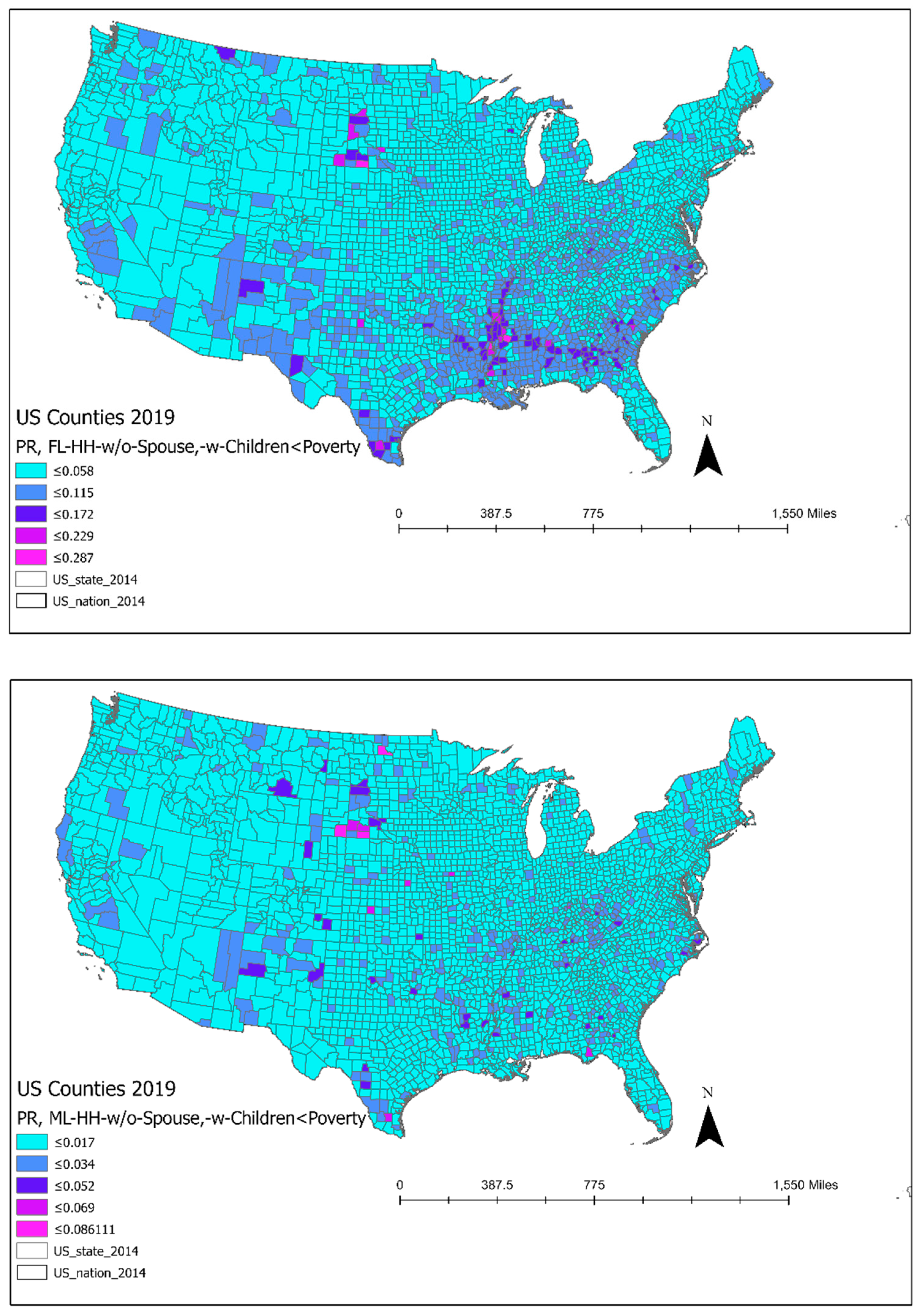
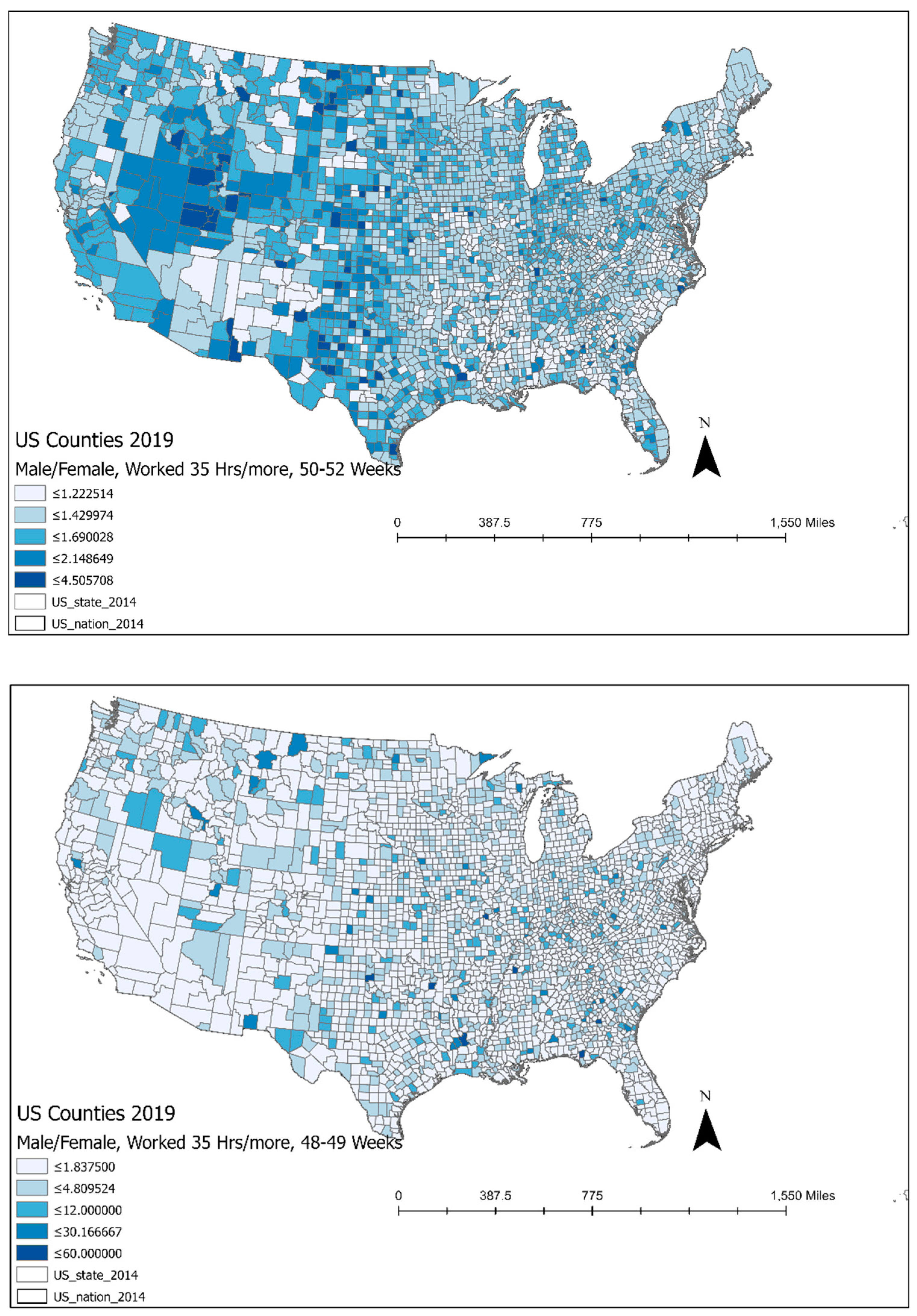
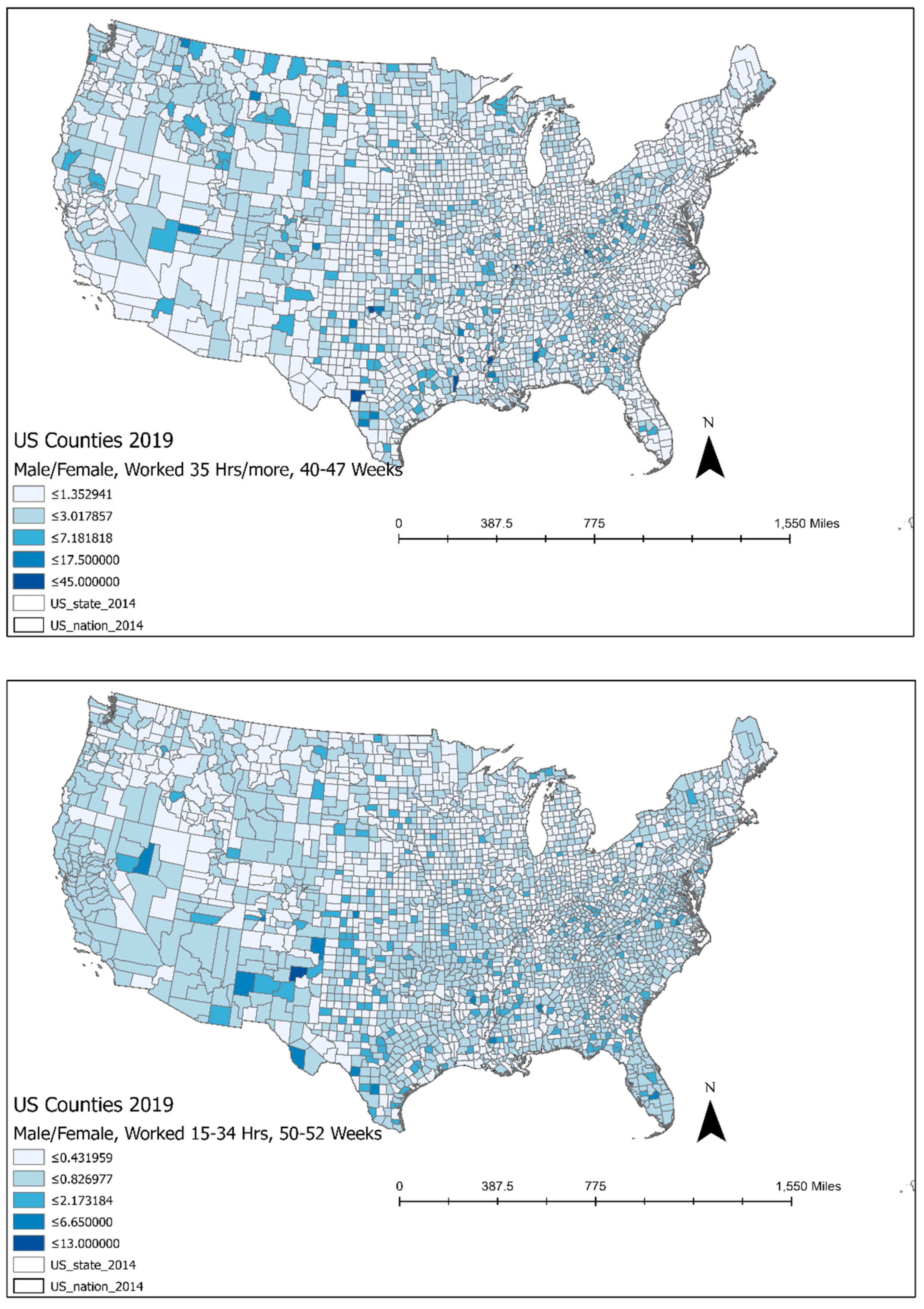
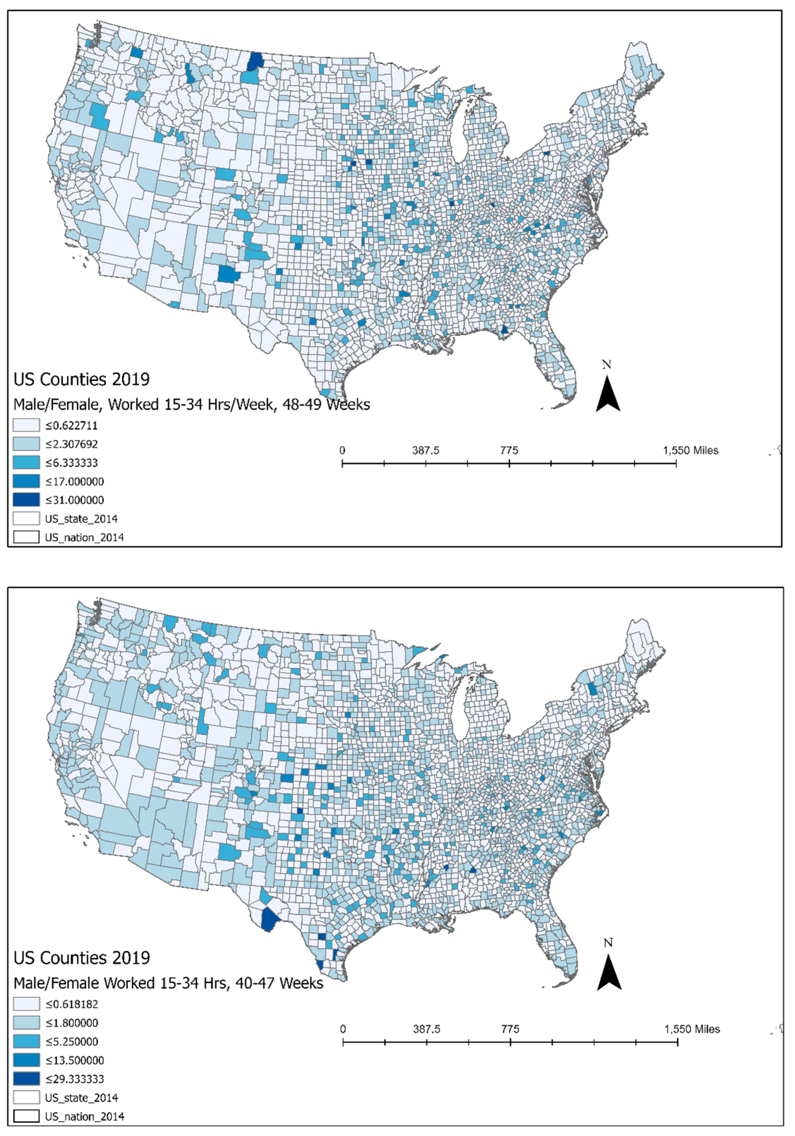
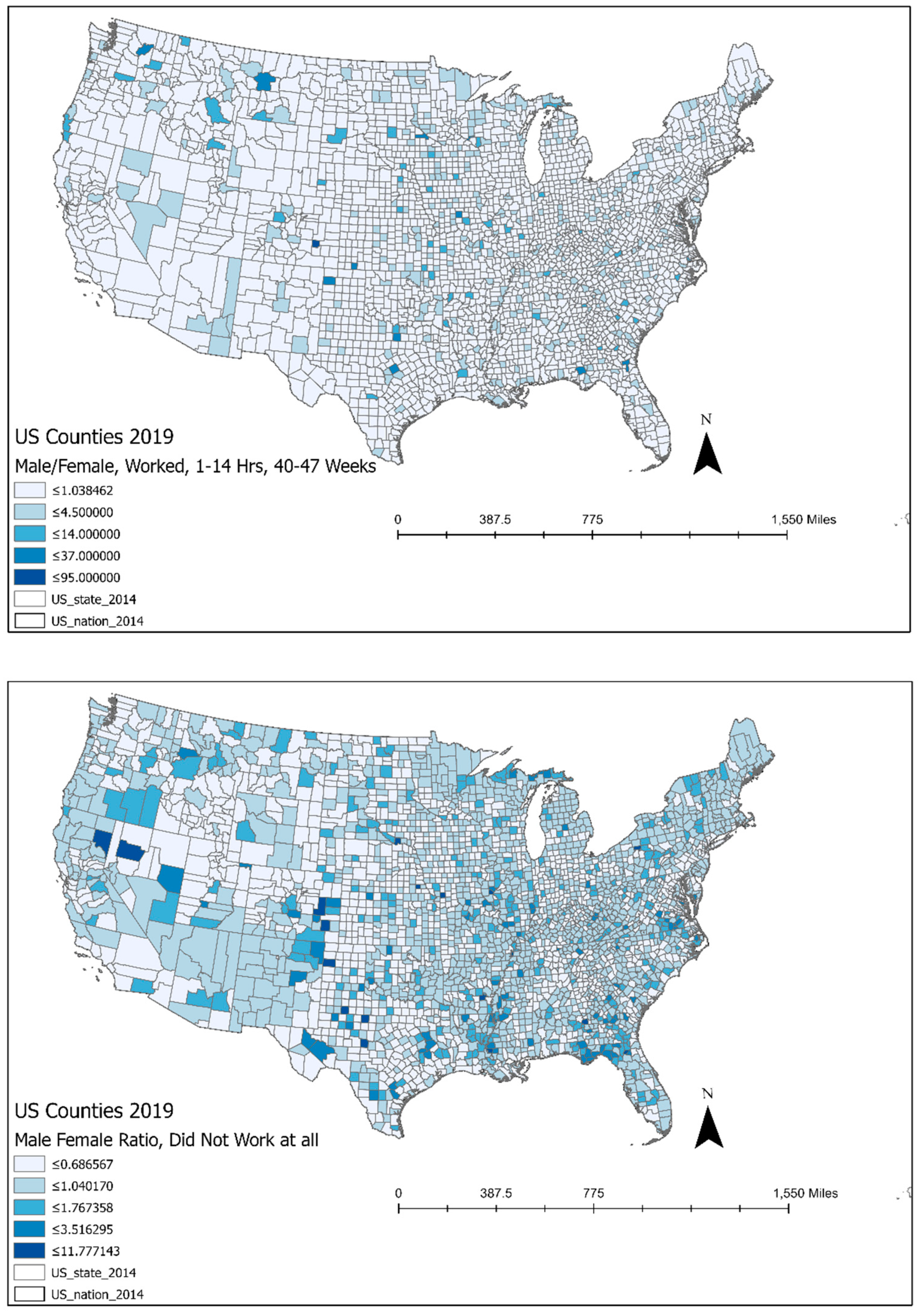
4.1. Visual Analysis of Major Variables: Gendered Poverty and Work Status

Choropleth maps were made for male-headed and female-headed households living in poverty (with children) and for select categories of male-to-female work status ratios and interpreted for their spatial patterns. As obvious from Figure 1, the female-headed households with children living in poverty have spatial clusters along the Mississippi Delta, the southeastern USA along the Black Belt, the Appalachian region, the Cotton Belt, southwestern USA, patches of central California where agriculture is the main occupation (Bakersfield, Portville, etc.), and random countries in other parts of the USA.

These patterns corroborate other prior research—with higher poverty in counties with relatively higher shares of diversity (largely blacks and Hispanics) and, as indicated by the Census reports, in random counties of reservations (Native Americans) [56,57,58]. The historical contexts of slavery and plantation economies and long decades of racial/ethnic discrimination, without doubt, have manifested into clusters of racialized poverty, and female-headed poverty shows up accordingly.

Figure 1. Female-headed and male-headed households with children living in poverty (no spouse), 2019.

Figure 1. Female-headed and male-headed households with children living in poverty (no spouse), 2019.

The male/female work-status ratios for those who worked above 35 h/week and other categories of work (≥35 h/week, 15–34 h/week, 1–14 h/week) for up to 40 weeks/year only are illustrated in Figure 2. The most obvious patterns emerging from a visual analysis of these maps are that as the number of hours worked/week decreases, the shades of blue become lighter and lighter—implying male advantage regarding full-time work status for the majority of the year (worked 40 weeks or more/year). The ratio of male/female work status for 1–14 h/week for up to 40 weeks/year, likewise, shows lighter shades of blue. Additionally, male/female ratios for those who did not work at all obtained a maximum value of 11.78, illustrated by the darkest blue counties (last map, Figure 2), which have a spatial randomness to them. However, some of these darkest shades of blue mirror the spatial patterns of overall poverty, with numerous counties along the Mississippi Delta, the Black Belt, Appalachia, and the like. A few of the random dark blue counties also show high poverty among the Native Americans. Finally, maps for those who worked less than 40 weeks/year are not presented here for brevity; likewise, maps for various categories of educational attainment, including majors in bachelor’s, and location quotients are also not presented here and are available upon request.

Figure 2. Male/female work ratios (≥35 h/week, 15–34 h/week, 1–14 h/week, did not work at all).

Figure 2. Male/female work ratios (≥35 h/week, 15–34 h/week, 1–14 h/week, did not work at all).

4.2. Educational Attainment across Gender, 2019

A basic descriptive analysis of the entire data indicates wide gaps in educational attainment across the genders, especially in STEM and professional disciplines (

Table 2. Educational attainment (A) and majors in bachelor’s (B) by gender, 2019.

A: Broad Categories, 25 Years/Older	Males		Females
	Mean	Max.	Mean	Max.
Share, No School at all	0.006	0.063	0.005	0.091
Share, No HS Diploma	0.065	0.343	0.055	0.393
Share, HS Diploma	0.179	0.437	0.163	0.272
Share, Some College/Associate	0.143	0.282	0.165	0.324
Share, Bachelor’s	0.066	0.251	0.077	0.204
Share, Master’s	0.023	0.148	0.034	0.144
Share, Professional	0.007	0.057	0.005	0.040
Share, Doctorate	0.005	0.137	0.003	0.040
B: Major in Bachelor’s Degree	Mean	Max.	Mean	Max.
Share, Science and Engineering	0.183	0.571	0.111	0.545
Share, Science and Engineering-related field	0.029	0.166	0.081	0.271
Share, Business	0.095	0.312	0.082	0.426
Share, Education	0.056	0.459	0.164	0.477
Share, Arts, Humanities, Others	0.088	0.750	0.109	0.432

A,B). The maximum values for males occur in the categories of High School Diploma, No High School Diploma, Some College/Associate; then those with Bachelor’s, Master’s, and Doctorate Degrees. In contrast, the maximum values for females occur for No High School diploma (39.3%), Some College/Associate (32.4%), High School diploma (27.2%), Bachelor’s (20.4%), Master’s (14.4%), Professional (4.0%), and Doctoral Degrees (4.0%). As is obvious from this table, males have significant advantage in terms of Doctoral and Bachelor’s Degrees, alongside High School Diplomas.

Concerning majors in a bachelor’s degree, the maximum values for females occur for science and engineering (54.5%), education (47.7%), arts/humanities/others (43.2%), business (42.62%), and science and engineering-related fields (27.1%); for these same majors, males have much higher maximum values in science and engineering, followed by education, business, and science and engineering-related fields. Mean values for these educational categories suggest higher percentages of women majoring in education (16.4%), arts/humanities (10.9%), science and engineering (11.1%), business (8.2%), and finally science and engineering-related (8.1%) disciplines (Table 2B). Men overwhelmingly major in science and engineering (18.3%), business (9.5%), arts/humanities (8.8%), education (5.6%), and lastly, science and engineering-related (2.8%) disciplines. These statistics are important to understand as the earnings capacity and poverty levels among men and women are intricately tied together. Even though the earnings and poverty levels of single women with children cannot be entirely explained by their educational attainment or skills, their different levels of education and skills are also manifestations of the societal, cultural, and policy contexts of a society, and I hope these will show up in the regression models with meaningful results.

4.3. Bivariate Correlations Analysis

The bivariate correlation analysis (

Table 3. Bivariate correlation analysis for female and male-headed households in poverty, with and without children and explanatory variables, 2019.

Explanatory Variables and Dependent Variables	Y1:FHwC	Y2:FHNC	Y3:MHwC
A: Share of Major Racial/Ethnic Groups (out of Total Population, 2019)
Non-Hispanic white	−0.539 **	−0.547 **	−0.202 **
Non-Hispanic black	0.597 **	0.622 **	0.102 **
Non-Hispanic American Indians	0.224 **	0.222 **	0.383 **
Non-Hispanic Asians-w-Hawaiian and Pacific Islanders	−0.120 **	−0.119 **	−0.099 **
Non-Hispanic All-Others	−0.043 *	−0.050 **	0.033
Hispanics	0.073 **	0.060 **	−0.004
B: Share, Educational Attainment and Majors in Bachelor’s Degree, Males and Females (≥25 Years)
No-School, Male	0.257 **	0.265 **	0.074 **
No High School, Male	0.471 **	0.497 **	0.264 **
High School Diploma, Male	0.163 **	0.175 **	0.210 **
Some College/Associate, Male	−0.311 **	−0.336 **	−0.118 **
Bachelor’s Degree, Male	−0.415 **	−0.431 **	−0.316 **
Master’s Degree, Male	−0.313 **	−0.320 **	−0.245 **
Professional Degrees, Male	−0.212 **	−0.214 **	−0.193 **
Doctorate, Male	−0.162 **	−0.157 **	−0.152 **
No School, Female	0.234 **	0.242 **	0.060 **
No High School, Female	0.525 **	0.546 **	0.282 **
High School Diploma, Female	0.204 **	0.214 **	0.167 **
Some College/Associate, Female	−0.110 **	−0.128 **	−0.036 *
Bachelor’s Degree, Female	−0.394 **	−0.413 **	−0.306 **
Master’s Degree, Female	−0.182 **	−0.186 **	−0.166 **
Professional Degrees, Female	−0.130 **	−0.123 **	−0.132 **
Doctorate, Female	−0.132 **	−0.130 **	−0.142 **
Science/Engineering, Male	−0.318 **	−0.324 **	−0.222 **
Science/Engineering-related field, Male	−0.02	−0.022	0.028
Business, Male	−0.025	−0.019	−0.123 **
Education, Male	−0.048 **	0.038 *	0.149 **
Arts/Humanities/Others, Male	−0.002	0.000	−0.025
Science/Engineering, Female	−0.114 **	−0.110 **	−0.079 **
Science/Engineering-related field, Female	−0.038 *	0.040 *	0.092 **
Business, Female	0.120 **	0.121 **	0.002
Education, Female	0.266 **	0.268 **	0.207 **
Arts/Humanities/Others, Female	−0.034	−0.034	−0.048 **
C: Location Quotients by Gender, Five Major Occupations
LQ-Male, Management, Business, Science and Arts	−0.410 **	−0.424 **	−0.260 **
LQ-Male, Service Occupations	0.203 **	0.217 **	0.174 **
LQ-Male, Sales and Office Occupations	−0.122 **	−0.121 **	−0.101 **
LQ-Male, Natural Resources, Construction and Maintenance	−0.038 *	−0.042 *	0.011
LQ-Male, Production, Transport, Material Moving	0.188 **	0.188 **	0.113 **
LQ-Female, Management, Business, Science and Arts	−0.135 **	−0.137 **	−0.083 **
LQ-Female, Service- Occupations	0.272 **	0.275 **	0.169 **
LQ-Female, Sales and Office Occupations	0.105 **	0.121 **	0.027
LQ-Female, Natural Resources, Construction and Maintenance	−0.018	−0.025	−0.029
LQ-Female, Production, Transport, Material Moving	0.216 **	0.221 **	0.098 **
D: Income Characteristics by Gender by Work Status (Inflation Adjusted), 2019
Median Household Income, Overall	−0.564 **	−0.585 **	−0.365 **
Median Household Income, Male, Overall	−0.441 **	−0.457 **	−0.305 **
Median Household Income, Male-Worked Fulltime	−0.421 **	−0.434 **	−0.275 **
Median Household Income, Male-Worked Parttime	−0.219 **	−0.224 **	−0.099 **
Median Household Income, Female, Overall	−0.340 **	−0.345 **	−0.213 **
Median Household Income, Female-Worked Fulltime	−0.394 **	−0.401 **	−0.225 **
Median Household Income, Female-Worked Parttime	−0.221 **	−0.229 **	−0.122 **
E: Share, Female Work Status: Hours Worked/Week, #of Weeks Worked/Year (Out of Total Labor)
Worked 35 h or more/Week, 50–52 Weeks/Year	−0.304 **	−0.328 **	−0.243 **
Worked 35 h or more/Week, 40–49 Weeks/Year	−0.143 **	−0.157 **	−0.072 **
Worked 35 h or more/Week, 14–39 Weeks/Year	0.074 **	0.060 **	0.064 **
Worked 35 h or more/Week, 1–13 Weeks/Year	0.124 **	0.118 **	0.099 **
Worked 15–34 h/Week, 50–52 Weeks/Year	−0.317 **	−0.345 **	−0.179 **
Worked 15–34/Week, 40-to-49 Weeks/Year	−0.249 **	−0.264 **	−0.149 **
Worked 15–34 h/Week, 14–39 Weeks/Year	0.074 **	0.060 **	0.064 **
Worked 15–34 h/Week, 1–13 Weeks/Year	−0.341 **	−0.357 **	−0.199 **
Worked 1–14 h/Week, 50–52 Weeks/Year	−0.208 **	−0.220 **	−0.112 **
Worked 1–14 h/Week, 40–49 Weeks/Year	−0.203 **	−0.210 **	−0.138 **
Worked 1–14 h/Week, 14–39 Weeks/Year	−0.271 **	−0.280 **	−0.172 **
Worked 1–14 h/Week, 1–13 Weeks/Year	−0.209 **	−0.222 **	−0.105 **
Did Not Work at all	0.513 **	0.550 **	0.303 **

Note: ** Correlation is significant at the 0.01 level (2-tailed); * Correlation is significant at the 0.05 level (2-tailed). Y1:FHwC: Share, Female-headed households—with children, living in poverty in 2019; Y2:FHNC: Share, Female-headed households—without children, living in poverty in 2019; Y3:MHwC: Share, Male-headed households—with children, living in poverty in 2019.

) shows that the presence of blacks and American Indians is associated with higher poverty levels for all three dependent variables, whereas the share of Hispanics is associated with higher poverty among female-headed households, both with and without children. These indicate the sad reality of contemporary American society, where female poverty and overall poverty have a very strong aspect of color to them—and these concern blacks, Hispanics, and Native Americans—as noted in the Census report as well [9]. Regarding education, in general, lower levels of education (high school diploma and below) associate with higher poverty for all three dependent variables; in contrast, better educational levels associate with lower poverty, albeit the strength of r-values depends on the major in a bachelor’s degree. Majoring in science and engineering among both genders is associated with lower poverty for all three dependent variables.

Concerning five major types of occupations, overrepresentation of males and females in service and production/transport/material moving is associated with higher poverty for all three dependent variables; the same holds true for females in sales/office occupations. Other occupation-types for both genders (management/professional and natural resources/construction) are associated with lower poverty for all dependent variables, though these are insignificant for LQ-values among females, likely due to their severe under-representation in this industry. Median household incomes (overall) and for males and females—all associate with lower poverty—as expected. Given its direct association with reducing poverty, I do not use any income variables in the regression models.

Regarding work status, in general, full-time working women have lower poverty rates with or without children, as is the case with men. As expected, the association is positive (i.e., higher poverty for female-headed households) for women working 39 weeks/year or less; so is the case with men—which is not surprising. Interestingly, women working 15–34 h/week and for 14–39 weeks/year are also associated with higher poverty. All other categories of work status for women are associated with lower poverty, which points toward the fact that a fuller work status for females is critical to alleviating female poverty, with or without children.

4.4. Regressions Models for Female-Headed and Male-Headed Households with Children in Poverty

After attempting OLS models with select variables of importance, I used the stepwise method to derive the best-fit regression model for each Y-variable. As noted in

Table 4. Regression models for female-headed households in poverty, with and without children (no spouse), 2019.

	Y: Share, Female-Headed Households in Poverty (With Children)				Y: Share, Female-Headed Households in Poverty (No Children)
Variables	B	Beta	t-Value	Sig.	B	Beta	t-Value	Sig.	VIF
(Constant)	0.014		1.696	0.090	0.016		1.748	0.081
Share, Non-Hispanic White	−0.090	−0.598	−19.283	0.000	−0.103	−0.586	−20.238	0.000	8.326
Share, Non-Hispanic Black	0.010	0.047	1.930	0.054	0.015	0.060	2.629	0.009	5.112
Share, Non-Hispanic Asians-w-Hawaiian/Pacific Islanders	−0.098	−0.098	−6.909	0.000	−0.101	−0.087	−6.555	0.000	1.745
Share, Non-Hispanic All Others	−0.086	−0.049	−3.646	0.000	−0.119	−0.058	−4.637	0.000	1.566
Share, Hispanics	−0.063	−0.285	−11.375	0.000	−0.078	−0.305	−13.054	0.000	5.415
Share, No High School, Female	0.289	0.264	15.612	0.000	0.345	0.270	13.713	0.000	3.847
Share, High School Diploma, Female	0.143	0.167	9.817	0.000	0.149	0.150	8.056	0.000	3.432
Share. Some College/Associate, Female	0.133	0.122	8.582	0.000	0.130	0.103	6.759	0.000	2.289
Share. Master’s Degree, Female	0.184	0.103	5.711	0.000	0.182	0.088	4.811	0.000	3.297
Share, Education, Female	0.047	0.091	6.831	0.000	0.050	0.084	6.676	0.000	1.554
LQ-Female, Service Occupations	0.035	0.153	12.117	0.000	0.043	0.159	13.215	0.000	1.438
LQ-Female, Management, Business, Sc. and Arts	0.068	0.189	10.389	0.000	0.084	0.201	11.791	0.000	2.879
LQ-Female, Production, Transport, Material Moving	0.023	0.123	8.226	0.000	0.028	0.126	8.882	0.000	2.006
LQ-Female, Sales and Office	0.024	0.075	5.964	0.000	0.034	0.093	7.888	0.000	1.379
Share, Females, Did Not Work at all	x	x	x	x	0.022	0.026	1.279	0.201	4.077
Share, Females, Worked 15–34 h/Week, 1–13 Weeks/Year	−0.164	−0.055	−4.254	0.000	−0.196	−0.056	−4.394	0.000	1.616
Share, Females, Worked ≥35 h/Week, 50–52 Weeks/Year	−0.182	−0.202	−15.850	0.000	−0.226	−0.215	−14.078	0.000	2.317
R-value	0.799				0.828
R-squared value	0.638				0.685
Adjusted R-square	0.636				0.683

, A and B, the presence of blacks, and the share of those with lower levels of education (i.e., no High School diploma, with high school diploma, some college/associate) receive positive Betas for female-headed households with children and without children living in poverty. These findings reiterate the effects of historical and contextual issues pertaining to race and gender in the USA, where limited educational outcomes particularly impact female poverty rates. The share of whites, Asians, Hispanics, and all other groups receive negative Betas, whereas the share of blacks receives positive Betas (0.047 and 0.060) in both models A and B. This is indicative of the intersectionality between race and gender, and given the positive Betas for blacks, it becomes more obvious that a large part of female poverty correlates strongly with the black population—implying higher poverty among black women. Higher poverty rates also corroborate strongly with the poverty clusters in Figure 1. Additionally, females with lower levels of educational skills are likely unable to translate them into better-paid jobs and financial well-being, and as noted in other research as well, having children pushes them further into poverty [8]. However, the share of females with a master’s degree also receives positive Beta for female-headed households in poverty, with and without children. This result is surprising, as one would expect better educated women to have a better capacity to safeguard against poverty. This new finding points toward the possibility that the presence of children and/or the single/divorced status of women might be extra stressors, even among the better educated. However, this will require further testing through targeted case studies.

When examining the majors in bachelor’s degrees among females, those majoring in education receive positive Beta—indicating higher poverty. Thus, “education” as a major is not the best way to safeguard against poverty, especially for single women, with or without children. This also points toward the fact that in the USA, teachers/education sector, generally perceived as feminine occupations, remain one of the lowest-paid occupations regardless of the instructor’s qualifications. Indeed, several media and news channels continue to run documentaries on the financial woes of teachers and how the schoolteachers work multiple jobs to make ends meet—largely because of their exceptionally low salaries.

The LQs in management, service, sales/office, and production/transportation-type occupations are associates with positive Betas, implying higher poverty levels among women engaged in these occupations. Some of these findings point toward the relative lower pay in these occupations, as noted in other work [6,7,8]. However, this new finding points toward the working poor—that section of society—largely the women who comprise an active labor force in the new econony and are living in poverty.

Regarding work status, it is a no-brainer that full-time work all throughout the year (35 h/week, 50–52 h/year) attributes toward reducing poverty among women (negative Beta), albeit the Beta is slightly stronger for single females compared to those with children. Even the share of females who worked only 15–34 h/week for 1–13 weeks/year also receives negative Beta, implying lower poverty. The share of females who did not work at all does not show up in the model for female-headed households with children, whereas this variable shows up for those without children but is insignificant. The R-Square values are very good for both models—0.638 (with children) and 0.685 (without children). The new findings from these models point toward the fact that full-time and even part-time work for single women helps reduce poverty, especially for those with children. Finally, the VIF values point toward some multicolliearity between major population groups (whites, blacks, and Hispanics), all of which are critical to measuring poverty in the entire country. Since removing them would drastically reduce the sample size and produce unreliable results, they were retained in the models.

When modeling male-headed households with children living in poverty (

Table 5. Regression Model for Male-Headed Households with Children in Poverty, 2019Y₃= Male Headed Households with Children in Poverty.

	B	Beta	t-Value	Sig.	VIF
(Constant)	0.042		14.469	0.000
Share, Non-Hispanic White	−0.026	−0.934	−12.782	0.000	17.414
Share, Non-Hispanic Black	−0.023	−0.532	−10.682	0.000	7.683
Share, Non-Hispanic Asians-w-Haw/Pacific Islanders	−0.036	−0.265	−8.682	0.000	2.338
Share, Hispanics	−0.023	−0.527	−10.109	0.000	8.848
Share, No High School, Male	0.038	0.180	5.987	0.000	2.177
Share, High School Diploma, Male	0.008	0.065	1.719	0.086	2.476
Share, Science and Engineering-Major, Male	−0.015	−0.107	−3.403	0.001	2.310
Share, Business Major, Male	−0.035	−0.182	−7.323	0.000	1.426
Share, Arts and Humanities Major, Male	−0.020	−0.078	−3.206	0.001	1.391
LQ-Male, Management, Business, Science and Arts	−0.010	−0.221	−5.010	0.000	3.155
LQ-Male, Service Occupations	0.006	0.122	4.704	0.000	1.605
LQ-Male, Nat-Resources, Construction and Maintenance	−0.003	−0.197	−6.527	0.000	2.166
M/F-Work-Ratio, ≥35 h/Week, 48–49 Weeks/Year	0.000	−0.077	−3.710	0.000	1.061
M/F-Work-Ratio, 1–14 h/Week, 50–52 Weeks/Year	0.000	0.056	2.696	0.007	1.047
M/F-Work-Ratio, 15–34 h/Week, 50–52 Weeks/Year	0.002	0.049	2.122	0.034	1.242
R-value	0.611
R-squared value	0.373
Adjusted R-square	0.367

Note: In this table, VIF has a high share of whites, blacks, and Hispanics. However, given their significant roles in predicting poverty and the size of their population in the entire sample, I kept them in the model.

), four major categories of race variables show up in the model, and they all receive negative Betas—implying lower poverty. The strength of Betas is strongest for whites (−0.934), followed by blacks (−0.532), Hispanics (−0.527), and Asians (−0.265). Regarding educational attainment, lower levels of education are associated with higher poverty and receive positive Betas, with no high school diploma having a stronger Beta (0.180) compared to a high school diploma (Beta = 0.065). Regarding majors in bachelor’s, science and engineering (Beta = −0.107), business (Beta = −0.182), and arts/humanities (Beta = −0.078) all associate with lower poverty, with the business major being the strongest.

Regarding occupation, LQ-management (Beta = −0.221) and LQ-natural resources, etc. (Beta = −0.197) associate with lower poverty for male-headed households with children, with management-type occupations having a stronger impact. LQ-Service, however, receives positive Beta (0.122), implying higher poverty—same as those for females (with or without children). What is clear and new from this model is that the over-presence of men in natural resource extraction/construction, etc. plays to their advantage, given its highly masculine nature and potential higher incomes. This research also finds new knowledge that being in management occupations protects single male-headed households with children from falling into poverty, whereas it does not in the case of female-headed households, with and without children.

Finally, the male-versus-female work status ratio for those who worked 35 h/more per week for 48–49 weeks/year associates with a negative Beta (lower poverty) whereas other two categories (1–14 h/week, 50–52 weeks/year, and 15–34 h/week, 50–52 weeks/year) representing part-time work status for males receive positive Betas, implying poverty, even though the strength of these Betas is small. This finding is new since the male/female ratios for part-time categories of work show a trend toward attaining parity with women, especially concerning poverty, which is an unpleasant situation. Finally, the R-square value for this model is 0.373, which is lower than 0.50. However, all the explanatory variables are significant and provide meaningful results. Regarding lower R-square values, scholars have suggested that it happens because of more noise in the data. Frost illustrates two different models to explain how the output does not change even when the R-square value is 0.147 (i.e., explaining only 14.7% of the variance) and that the higher variability of data around the regression slope line is what produces a lower R-squared value [59]. In the past, numerous scholars who have worked on rural women’s livelihoods and economic patterns in Bangladesh have published their results with lower R-squared values, explaining 11–13% of total variance [60,61]. In this study, the R-square value is far better, and the explanatory variables provide meaningful results.

5. Conclusions and Policy Implications

This analysis aimed at examining varying levels of poverty among male- and female-headed households, with and without children, living in poverty in the counties in the USA. By using a multi-level empirical analysis of county-scale five-year ACS estimates from the NHGIS, this analysis finds some expected and some surprising results. Sadly, the presence of black population associates with higher levels of poverty (positive Betas) for female-headed households, with and without children, whereas most of the race variables associate with lower levels of poverty (negative Beta) for male-headed households with children. This points toward the fact that a large part of female poverty is likely due to the larger share of black women in the black population being captured in positive Betas in the model.

This analysis also finds that, in general, lower levels of education (some college/associate degree or lower) are associated with higher poverty for both genders. One new finding from this analysis is that for females with a master’s degree, the Beta is positive—hinting toward the presence of children and/or their single status as the “stressors” of poverty. This finding, however, will need further investigation through a case study/qualitative approach. This research also finds that for females, majoring in education does not provide a pathway toward alleviating poverty. Indeed, for a long time, the lower salary of teachers specifically has remained a widely discussed topic in news channels/media in the US. At the policy level, raising the salary of teachers and providing them with other benefits is critical, as many women work as educators, and timely intervention will help reduce poverty and create a more equitable society. For males, majoring in science and engineering, business, and the arts/humanities—all associated with lower poverty—and the strength of business was the highest. This points toward the fact that encouraging more women to major in science, engineering, and business could be a potential pathway toward alleviating poverty and achieving equity. This was also emphasized at the most recent convention of the United Nations, where it was emphasized that even though 75% of all job growth will be in STEM-related disciplines, women comprise only 30% of the global workforce in the world’s 20 largest global tech companies [17]. This gap in educational and human capital skills needs to be narrowed, as this is the only pathway toward creating a just and equitable future by 2030 and achieving the UN’s SDGs [17]. In the U.S., this needs policy-level intervention so that universities can provide special scholarships to attract female students into science and engineering, business, and other professional degrees/majors. Further, recruitment of graduated female students by employers at local, regional, and national levels could be encouraging steps toward achieving equity and reducing female poverty.

In terms of relationships between poverty and gender-based occupations, the service sector is associated with higher poverty for both genders, regardless of children’s presence at home. For male-headed households, however, management and natural resources/construction-based occupations are associated with lower poverty, but management has a stronger role. For women, however, management, sales/office, and service-type occupations—all associated with higher poverty—point toward the emergence of a new class—the “working poor”—largely comprised of women—an active part of the contemporary US labor force and yet living in poverty.

These findings point toward a sad reality of the US labor market where similar types of occupations yield different levels of earnings (and poverty) across the genders, with males having an advantage in specific industries and with specific educational backgrounds. This finding reemphasizes the role of Labor Market Segment Theory in capturing the subtle/unwritten rules that still prevail in specific industries where females are systemically paid lower wages compared to males. This research also adds a new dimension to the Human Capital Theory since majoring in “Education” does not yield enough earnings to single females (with and without children both) to reduce poverty, whereas majoring in science and engineering, business, and arts/humanities works quite well for single males with children. I call it the “Neo-Human Capital Theory”, which accounts for gender-based variations in skills and earnings by adequately weighing regional and cultural variations.

In terms of policy, these findings call for the state and federal governments’ legal intervention in ensuring equal pay for equal work in the U.S. labor market. Implementing these can be very challenging in a large and diverse country such as the USA. However, this is the only pathway toward ensuring gender equality in earnings and lowering poverty for women, especially for those with children. Single parents/single female headed households with children are the reality of contemporary America. Ensuring legal protection for “equal pay for equal work” can provide a decent upbringing to the children involved in such families—a critical necessity toward creating a healthier society and a healthy nation. This is the only way forward toward attaining the SDGs of the United Nations.

In terms of work status, higher male-female ratios for those working more than 35 h/week, 48–49 weeks/year, were associated with lower poverty for males, whereas for females, the share of females working 35 h/more, 50–52 weeks/year, worked toward alleviating poverty. Both of these cases are not surprising as they point toward fuller work status for both genders. However, what is surprising is that part-time work status for females also associates with lower poverty, albeit at reduced strength compared to full-time work status; in contrast, the male/female work status ratios in part-time categories associate with higher poverty for males—pointing toward an “equalizing” trend regarding poverty. This finding is concerning, especially since some men might have to work part-time to accommodate specific needs, but its eventual manifestation in terms of heightened poverty might have opposing effects.

In terms of policy, this research reemphasizes the need for creating opportunities for full-time employment for both genders, and more specifically for females, due to the positive contribution of full-time employment to alleviating poverty. This implies providing subsidized care facilities, family/maternity leave benefits, flexible work hours, tax credits for families with children, and other types of gender-inclusive work environments such that women can participate fully in the labor market and are able to focus on their work and family both without any feeling of guilt. This will ensure a happier and more positive work culture, and women will be able to contribute to the economy without worrying about the “motherhood penalty” and the consequential restricted/limited career growth.

This study, despite its new and interesting findings, has some limitations. Creating a good R-square model for males with children was difficult due to the scattered nature of the data points. This highlights the noise in the ACS estimates, likely due to the difficulties in measuring and capturing the socioeconomic and labor-market variables—most of which are private information. Other limitations include the difficulties in assessing the reasons that produce different poverty outcomes for males and females with similar types of educational backgrounds. These point toward the limitations of the data in capturing cultural and regional nuances. These can be remedied to some extent by adopting mixed-methods/qualitative approaches, which are time-consuming, case-specific, and not generalizable. Given the size of the data analyzed in this study and weighing the pros and cons of quantitative versus qualitative methods, these limitations outweigh the science and knowledge gained in this research.

References

1. HTTP1. Gender Equality Will Take 300 Years to Achieve, Says UN Chief, Business Standard, 9 March 2023. Available online: https://www.business-standard.com/article/printer-friendly-version?article_id=123030900003_1 (accessed on 16 March 2023).
2. Darden, J.T.; Rahbar, M.; Jezierski, L.; Li, M.; Velie, E. The measurement of neighborhood socioeconomic characteristics and black and white residential segregation in metropolitan Detroit: Implications for the study of social disparities in health. Ann. Assoc. Am. Geogr. 2010, 100, 137–158. [Google Scholar] [CrossRef]
3. Essletzbichler, J. The top 1% in U.S. metropolitan areas. Appl. Geogr. 2015, 61, 35–46. [Google Scholar] [CrossRef]
4. Kawachi, I. Social capital and community effects on population and individual health. Ann. N. Y. Acad. Sci. 2006, 896, 120–130. [Google Scholar] [CrossRef]
5. Glynn, S.J. Gender Wage Inequality: What We Know and How We Can Fix It; Center for Equitable Growth Report; Washington Center for Equitable Growth: Washington, DC, USA, 2018. [Google Scholar]
6. Sharma, M. Multiple Dimensions of Gender (Dis)Parity: A County-Scale Analysis of Occupational Attainment in the USA, 2019. Sustainability 2021, 13, 8915. [Google Scholar] [CrossRef]
7. Sharma, M. Gender Disparity and Economy in US Counties: Change and Continuity, 2000–2017. In Gender Inequalities: GIS Approaches to Gender; Ozdenerol, E., Ed.; CPC Press: Abingdon, UK, 2020; pp. 73–96. ISBN 9780367184735. Available online: https://www.routledge.com/Gender-Inequalities-GIS-Approaches-to-Gender-Analysis/Ozdenerol/p/book/9780367184735 (accessed on 2 February 2023).
8. Sharma, M. Gendered Dimensions of Educational Premium Disadvantage in Earnings in USA, 2019. GeoJournal 2022, 87, 847–868. [Google Scholar] [CrossRef] [PubMed]
9. HTTP2: Income and Poverty in the United States: Highlights, 2020. Available online: https://www.census.gov/library/publications/2021/demo/p60-273.html (accessed on 15 March 2023).
10. Manson, S.; Schroeder, J.; Van Riper, D.; Kugler, T.; Ruggles, S. IPUMS National Historical Geographic Information System: Version 15.0; IPUMS: Minneapolis, MN, USA, 2020. [Google Scholar] [CrossRef]
11. HTTP3. Available online: https://inequality.org/our-inequality-work/ (accessed on 10 March 2023).
12. HTTP4. Available online: https://inequality.org/our-inequality-work/reports-2/ (accessed on 9 March 2023).
13. Islam, F.B.; Sharma, M. Gendered dimensions of unpaid activities: An empirical insight into rural Bangladesh households. Sustainability 2021, 13, 6670. [Google Scholar] [CrossRef]
14. Islam, F.B.; Sharma, M. Socio-economic determinants of women’s livelihood time use in rural Bangladesh. GeoJournal 2022, 87, 439–451. [Google Scholar] [CrossRef]
15. HTTP5. U.S. Department of Labor. Available online: https://fortune.com/tag/u-s-department-of-labor/ (accessed on 2 February 2023).
16. Gould, E.; Schieder, J.; Geier, K. What is the gender pay gap and is it real? The complete guide to how women are paid less than men and why it can’t be explained away. Econ. Policy Res. Rep. 2016, 20, 1–41. [Google Scholar]
17. HTTP6. United Nations News on Gender Equality: International Women’s Day Puts the Spotlight on Digital Gender Equality. Available online: https://news.un.org/en/story/2023/03/1134342 (accessed on 17 March 2023).
18. Piketty, T.; Saez, E.; Zucman, G. Replication Data for: ‘Distributional Accounts: Methods and Estimates for the United States’, Harvard Dataverse, 2017. Available online: https://dataverse.harvard.edu/dataset.xhtml?persistentId=doi:10.7910/DVN/SLXCUJ (accessed on 2 February 2023).
19. Chari, A.; Goldsmith-Pinkham, P. Gender Representation in Economics across Topics and Time: Evidence from the NBER Summer Institute; Working Paper 23953; National Bureau of Economic Research: Cambridge, MA, USA, 2017; Available online: http://www.nber.org/papers/w23953 (accessed on 18 March 2023).
20. Whitmore, D.S.; Ryan, N. The 51%: Driving Growth through Women’s Economic Participation; Brookings Report, 2017. Available online: https://www.hamiltonproject.org/publication/policy-book/the-51-driving-growth-through-womens-economic-participation/ (accessed on 2 February 2023).
21. Census 2020 Report, The Bureau of U.S. Census 2020. Income and Poverty Report, 2020; The Bureau of U.S. Census: Suitland-Silver Hill, MD, USA, 2020.
22. Coe, N.M.; Kelly, P.F.; Yeung, H.W.C. Economic Geography: A Contemporary Introduction, 3rd ed.; Wiley Blackwell: Hoboken, NJ, USA, 2019; ISBN 978-1-119-38955-2. [Google Scholar]
23. International Labour Organization (ILO). More than 60 per Cent of the World’s Employed Population Are in the Informal Economy. 2018. Available online: www.ilo.org/global/about-the-ilo/newsroom/news/WCMS_627189/lang--en/index.htm (accessed on 13 March 2023).
24. International Labour Organization (ILO). Women do 4 Times More Unpaid Care Work than Men in Asia and the Pacific, 2018. Available online: https://www.ilo.org/asia/media-centre/news/WCMS_633284/lang--en/index.htm (accessed on 13 March 2023).
25. Charmes, J. The Unpaid Care Work and the Labour Market. An Analysis of Time Use Data Based on the Latest World Compilation of Time-Use Surveys; International Labour Office: Geneva, Switzerland, 2019. [Google Scholar]
26. WCR. Washington Center Report (2019) on Gender Wage Inequality in the United States: Causes and Solutions to Improve Family Well-being and Economic Growth, (2019); Washington Center for Equitable Growth Report; Washington Center for Equitable Growth: Washington, DC, USA, 2019. [Google Scholar]
27. CPS ASEC; U.S. Census Bureau. Current Population Survey 2019 and 2020 Annual Social and Economic Supplements (CPS ASEC); U.S. Census Bureau: Suitland-Silver Hill, MD, USA, 2020. [Google Scholar]
28. Collinson, C. Here and Now: How Women Can Take Control of Their Retirement. 2018. Available online: https://www.transamericacenter.org/docs/default-source/women-and-retirement/tcrs2018_sr_women_take_control_of_retirement.pdf: (accessed on 13 March 2023).
29. Autor, D.; Katzl, F.; Kearney, M. The Polarization of the U.S. Labor Market; NBER Working Paper Series No. 11986; National Bureau of Economic Research Papers: Cambridge, MA, USA, 2006; Available online: http://www.nber.org/papers/w11986 (accessed on 13 March 2023).
30. Berube, A. All Cities Are Not Created Unequal, Brookings Quality Independent Impact Report, 2013. Available online: https://www.brookings.edu/research/all-cities-are-not-created-unequal/ (accessed on 10 February 2023).
31. Kearney, M.S. Testimony before the Joint Economic Committee: Income Inequality in the United States. Kearney JEC Testimony. 2014, pp. 1–10. Available online: https://www.brookings.edu/wp-content/uploads/2016/06/16-income-inequality-in-america-kearney-1.pdf (accessed on 10 February 2023).
32. Nichols, A. Poverty in the United States. Urban Institute Fact Sheet. 2013. Available online: https://www.urban.org/sites/default/files/publication/23971/412898-poverty-in-the-united-states.pdf (accessed on 10 February 2023).
33. Sassen, S. Cities in a World Economy; Sage: Thousand Oaks, CA, USA, 1994. [Google Scholar]
34. Bakshi, P.; Goodwin, M.; Painter, J.; Southern, A. Gender, race, and class in the local welfare state: Moving beyond regulation theory in analyzing the transition from Fordism. Environ. Plan. A 1995, 27, 1539–1554. [Google Scholar] [CrossRef]
35. Brenner, N. Decoding the newest “metropolitan regionalism” in the USA: A critical overview. Cities 2002, 19, 3–21. [Google Scholar] [CrossRef]
36. Florida, R.; Mellander, C. The geography of Inequality: Difference and determinants of wage and income inequality across US metros. Reg. Stud. 2014, 50, 79–92. [Google Scholar] [CrossRef]
37. Gartman, D. Postmodernism; or, the cultural logic of post-Fordism? Sociol. Q. 1998, 39, 119–137. [Google Scholar] [CrossRef]
38. Moore, J. Documentary. Roger and Me. 1989. Available online: https://www.youtube.com/watch?v5L8jhqrQRhrY (accessed on 10 February 2023).
39. Walks, A. The social ecology of the post-Fordist/global city? Economic restructuring and socio-spatial polarization in the Toronto urban region. Urban Stud. 2001, 38, 407–447. [Google Scholar] [CrossRef]
40. Glaeser, E.L.; Resseger, M.G.; Tobio, K. Urban Inequality. NBER Working Paper Series 2008, Working Paper # 14419. Available online: http://www.nber.org/papers/w14419 (accessed on 10 February 2023).
41. Hamoudi, A.A.; Sachs, J.D. Economic Consequences of Health Status: A Review of the Evidence; Working Paper No. 30; Center for International Development at Harvard University: Cambridge, MA, USA, 1999. [Google Scholar]
42. Pink-Harper, S.A. Educational Attainment: An examination of its impact on regional economic growth. Econ. Dev. Q. 2015, 29, 167–179. [Google Scholar] [CrossRef]
43. Porter, M.E. Inner-city economic Development: Learnings from 20 Years of research and practice. Econ. Dev. Q. 2016, 30, 105–116. [Google Scholar] [CrossRef]
44. Autor, D.; Katzl, F.; Krueger, A. Computing inequality: Have computers changed the labor market? Q. J. Econ. 1998, 113, 1169–1213. [Google Scholar] [CrossRef]
45. Autor, D.; Levy, F.; Murnaner, R. The skill content of recent technological change: An empirical exploration. Q. J. Econ. 2003, 118, 1279–1333. [Google Scholar] [CrossRef]
46. Chakravorty, S. Urban inequality revisited: The determinants of income distribution in U.S. metropolitan areas. Urban Aff. Rev. 1996, 31, 759–777. [Google Scholar] [CrossRef]
47. Walks, A.; Maaranen, R. Gentrification, social mix, and social polarization: Testing the linkages in large Canadian Cities. Urban Geogr. 2008, 29, 293–326. [Google Scholar] [CrossRef]
48. Becker, G.S. Human Capital: A Theoretical and Empirical Analysis, with Special Reference to Education, 3rd ed.; University of Chicago Press: Chicago, IL, USA, 1994; 412p, ISBN 9780226041209. [Google Scholar]
49. Bonds, A. Racing Economic Geography: The Place of Race in Economic Geography. Geogr. Compass 2013, 7, 398–411. [Google Scholar] [CrossRef]
50. Mollett, S. Environmental struggles are feminist struggles: Feminist political ecology as development critique. In Feminist Spaces: Gender and Geography in a Global Context; Oberhauser, A.M., Fluri, J.L., Whitson, R., Mollett, S., Eds.; Routledge: New York, NY, USA, 2018; pp. 155–187. [Google Scholar]
51. Nightingale, A. The nature of gender: Work, gender, and environment. Environ. Plan. D Soc. Space 2006, 24, 165–185. [Google Scholar] [CrossRef]
52. Rocheleau, D.; Thomas-Slayter, B.; Wangari, E. Feminist Political Ecology: Global Issues and Local Experiences; CPC Press: London, UK, 1996; p. 164. ISBN 0415120268. [Google Scholar]
53. Ross, H. Feminist Political Ecology: Global Issues and Local Experiences. Dianne Rocheleau, Barbara Thomas Slayter and Esther Wangari (eds) London and New York: Routledge, 1996. Reviewed by Helen Ross. J. Political Ecol. 1997, 4, 21. [Google Scholar]
54. Sultana, F. Gendering Climate Change: Geographical Insights; Taylor and Francis: London, UK, 2014; Volume 66, pp. 372–381. [Google Scholar]
55. Moineddin, R.; Beyene, J.; Boyle, E. On the location quotient confidence interval. Geogr. Anal. 2003, 35, 249–256. [Google Scholar] [CrossRef]
56. Sharma, M. Spatial Perspectives on Diversity and Economic Growth in Alabama, 1990–2011. Southeast. Geogr. 2016, 56, 329–354. [Google Scholar] [CrossRef]
57. Sharma, M. Race, Place and Persisting Income Divide in the U.S. Southeast, 2000–2014. Growth Chang. 2017, 48, 570–589. [Google Scholar] [CrossRef]
58. Sharma, M. Change and Continuity of Income Divide in the American Southeast: A Metropolitan Scale Analyses, 2000–2014. Appl. Geogr. 2017, 88, 186–198. [Google Scholar] [CrossRef]
59. Frost, J. How to Interpret Regression Models that have Significant Variables but a Low R-Squared. Available online: https://statisticsbyjim.com/regression/low-r-squared-regression/ (accessed on 20 April 2023).
60. Chowdhury, S.K. Impact of infrastructures on paid work opportunities and unpaid work burdens on rural women in Bangladesh. J. Int. Dev. 2010, 22, 997–1017. [Google Scholar] [CrossRef]
61. Seymour, G.; Floro, M. Identity, Household Work, and Subjective Well-Being among Rural Women in Bangladesh; IFPRI Discussion Paper 01580; 2016. Available online: https://www.ifpri.org/publication/identity-household-work-and-subjective-well-being-among-rural-women-bangladesh (accessed on 1 March 2020).