
Prediction of the Tunnel Collapse Probability Using SVR-Based Monte Carlo Simulation: A Case Study

Abstract
1. Introduction
2. Theory and Methodology
2.1. Strength Reduction Method and the Failure Criterion
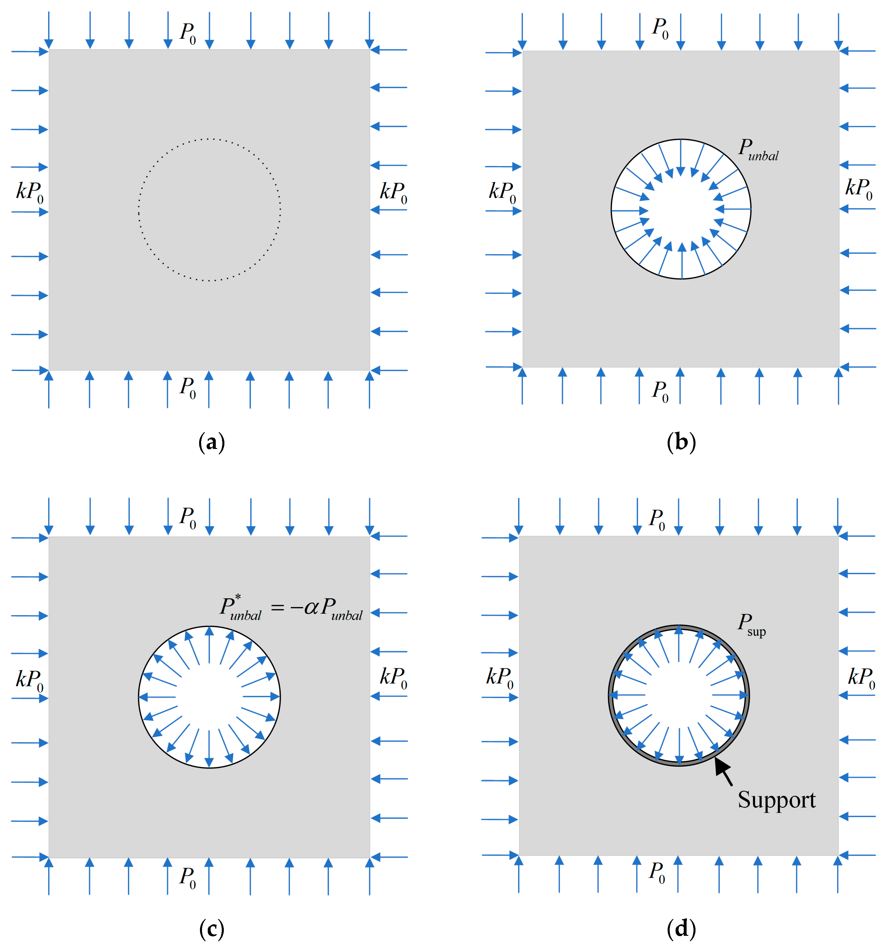
2.2. Stress Release Method for Support Timing Control
2.3. The Monte Carlo Method
2.4. Support Vector Regression
2.5. Collapse Risk Prediction Method
- (1)
- Several parameters are selected as random variables based on the actual conditions of the project. Then, a series of safety factors of the surrounding rock, derived from the FLAC3D simulations, are utilized as training data for SVR.
- (2)
- The SVR model with ideal performance is obtained through the training process, and a nonlinear mapping between random variables and safety factors is established to replace the performance function of the Monte Carlo method.
- (3)
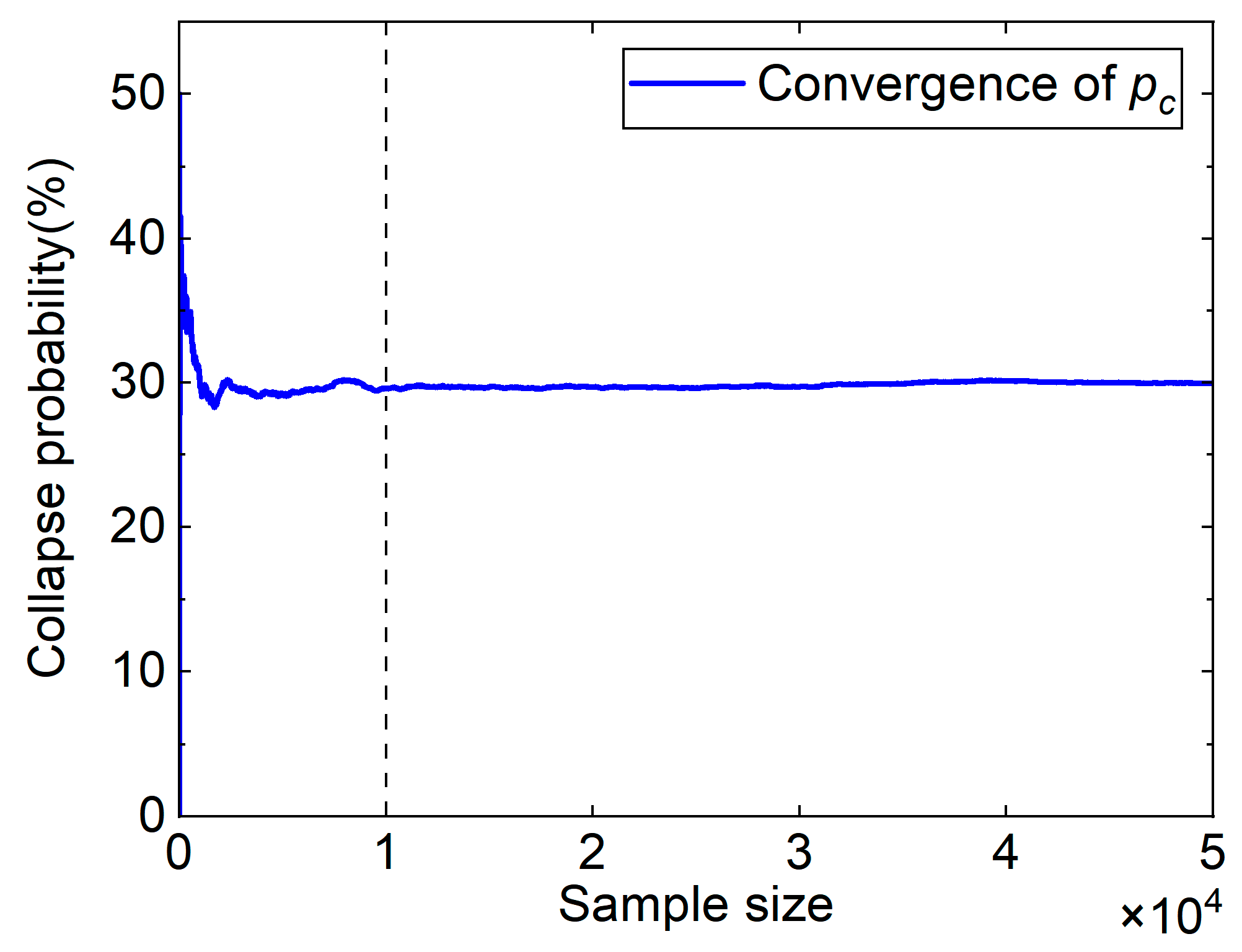
- The reliability model for the problem is established and a limit state function is defined. Then, the number of random samples required for the MC method are determined to ensure probability convergence.
- (4)
- The required number of random samples are generated and fed into a well-trained SVR model to execute the MC simulation. The number of random samples that fall into the failure domain is counted according to the limit state function, and the approximate failure probability, i.e., the collapse probability, can be obtained by Equation (3).
3. Case Study
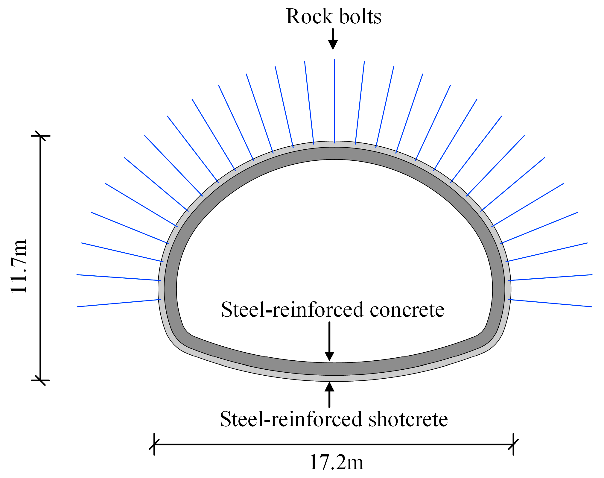
3.1. Overview of the Tunnel Excavation Project
3.2. Numerical Modeling and Validation
3.3. Stability Analysis of the Surrounding Rock
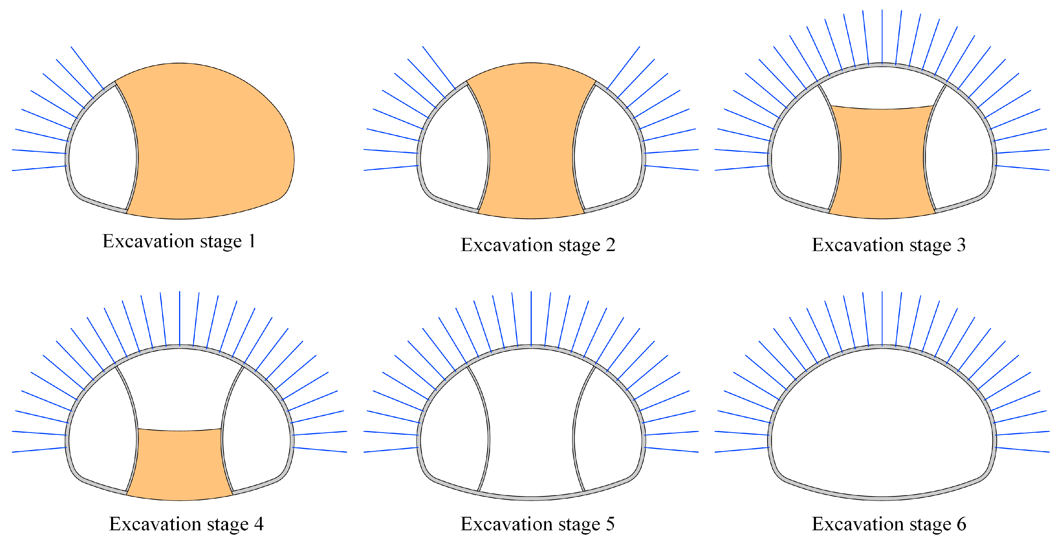
3.3.1. Simulation Scheme
3.3.2. Calculation of Safety Factors
3.4. Generating Data Set
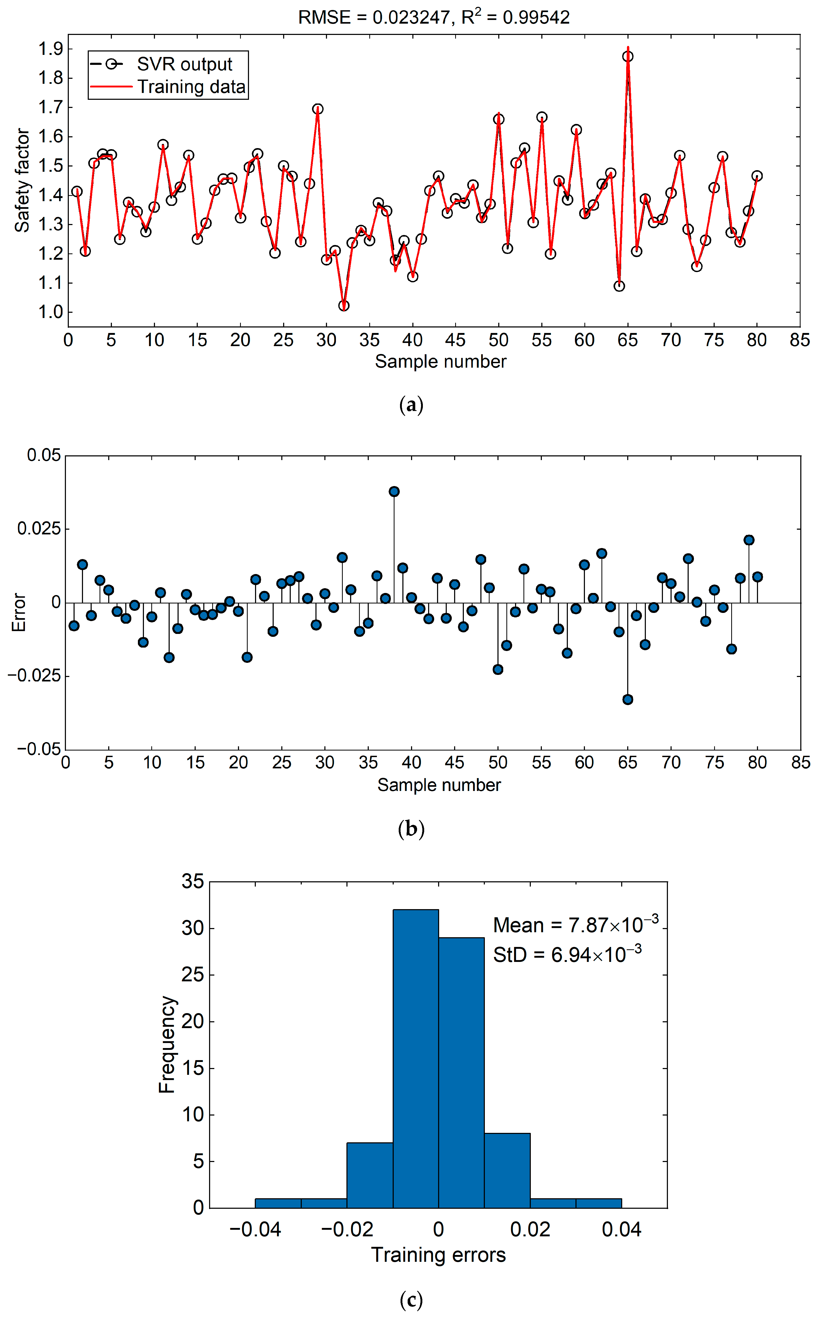
3.5. SVR Training for Safety Factor Prediction
3.6. Collapse Probability Calculation
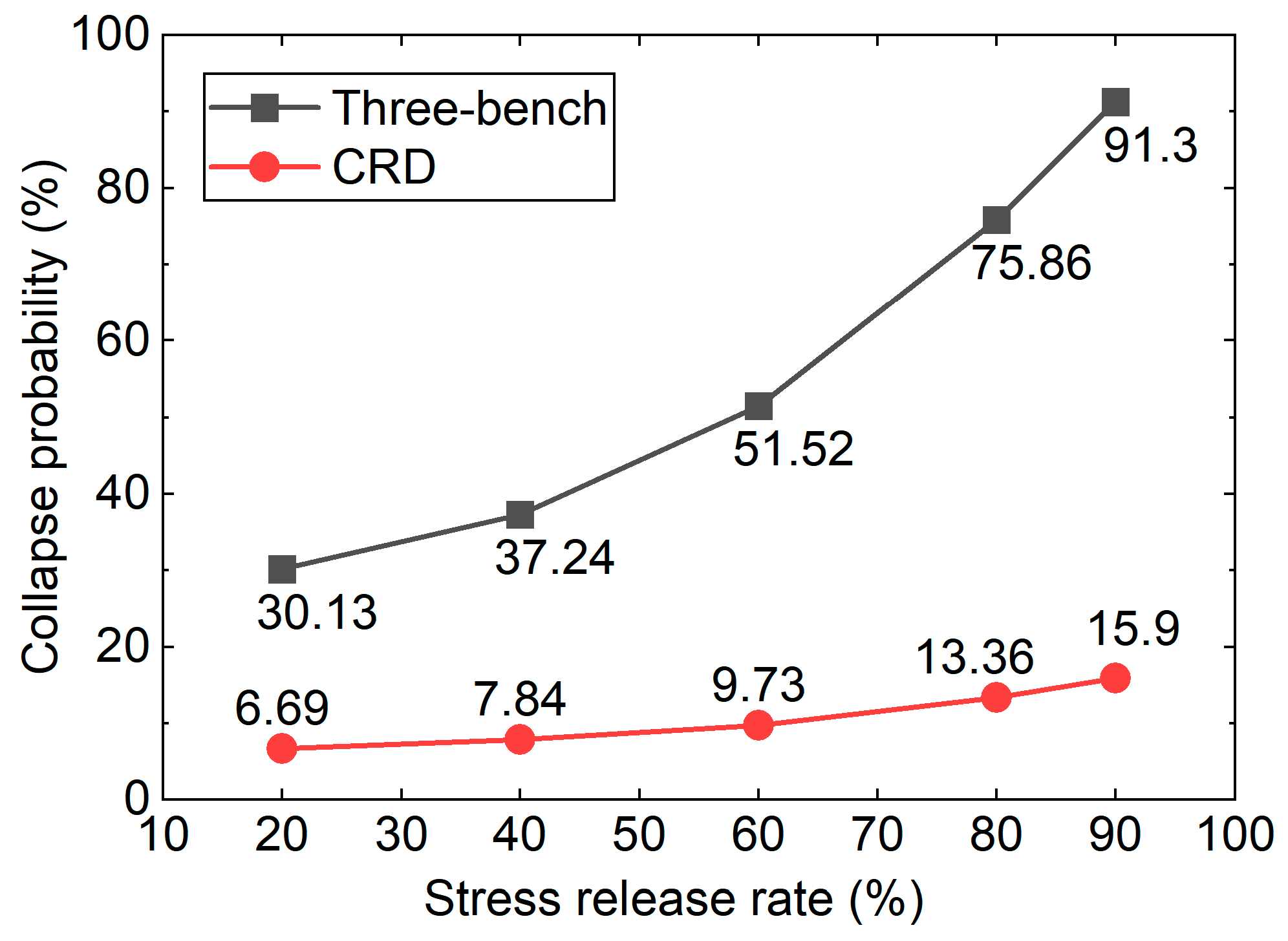
3.7. Result Analysis and Validation
4. Discussion
5. Conclusions
Author Contributions
Funding
Institutional Review Board Statement
Informed Consent Statement
Data Availability Statement
Conflicts of Interest
References
- Hong, K.R.; Feng, H.H. Development Trends and Views of Highway Tunnels in China over the Past Decade. China J. Highw. Transp. 2020, 33, 62–76. [Google Scholar]
- Wang, X.L.; Lai, J.X.; Qiu, J.L.; Xu, W.; Wang, L.X.; Luo, Y.B. Geohazards, reflection and challenges in Mountain tunnel construction of China: A data collection from 2002 to 2018. Geomat. Nat. Hazards Risk 2020, 11, 766–785. [Google Scholar] [CrossRef]
- Ou, G.; Jiao, Y.; Zhang, G.; Zou, J.; Tan, F.; Zhang, W. Collapse risk assessment of deep-buried tunnel during construction and its application. Tunn. Undergr. Space Technol. 2021, 115, 104019. [Google Scholar] [CrossRef]
- Xu, Z.G.; Cai, N.G.; Li, X.F.; Xian, M.T.; Dong, T.W. Risk assessment of loess tunnel collapse during construction based on an attribute recognition model. Bull. Eng. Geol. Environ. 2021, 80, 6205–6220. [Google Scholar] [CrossRef]
- Sharafat, A.; Latif, K.; Seo, J. Risk analysis of TBM tunneling projects based on generic bow-tie risk analysis approach in difficult ground conditions. Tunn. Undergr. Space Technol. 2021, 111, 103860. [Google Scholar] [CrossRef]
- Sun, J.L.; Liu, B.G.; Chu, Z.F.; Chen, L.; Li, X. Tunnel collapse risk assessment based on multistate fuzzy Bayesian networks. Qual. Reliab. Eng. Int. 2018, 34, 1646–1662. [Google Scholar] [CrossRef]
- Ou, X.D.; Wu, Y.F.; Wu, B.; Jiang, J.; Qiu, W.X. Dynamic Bayesian Network for Predicting Tunnel-Collapse Risk in the Case of Incomplete Data. J. Perform. Constr. Facil. 2022, 36, 04022034. [Google Scholar] [CrossRef]
- Li, F.Y. Research on Tunnel Collapse Risk Prediction and Control. Master’s Thesis, Central South University, Changsha, China, 2011. [Google Scholar]
- Wu, B.; Qiu, W.X.; Huang, W.; Meng, G.W.; Nong, Y.; Huang, J.S. A Multi-Source Information Fusion Evaluation Method for the Tunneling Collapse Disaster Based on the Artificial Intelligence Deformation Prediction. Arab. J. Sci. Eng. 2022, 47, 5053–5071. [Google Scholar] [CrossRef]
- Paternesi, A.; Schweiger, H.F.; Scarpelli, G. Numerical analyses of stability and deformation behavior of reinforced and unreinforced tunnel faces. Comput. Geotech. 2017, 88, 256–266. [Google Scholar] [CrossRef]
- Hu, X.Y.; Fu, W.; Wu, S.Z.; Fang, Y.; Wang, J.; He, C. Numerical study on the tunnel stability in granular soil using DEM virtual air bag model. Acta Geotech. 2021, 16, 3285–3300. [Google Scholar] [CrossRef]
- Yu, W.B.; Zhang, T.Q.; Lu, Y.; Han, F.L.; Zhou, Y.F.; Hu, D. Engineering risk analysis in cold regions: State of the art and perspectives. Cold Reg. Sci. Technol. 2020, 171, 102963. [Google Scholar] [CrossRef]
- Xiong, Z.M.; Lu, H.; Wang, M.Y.; Qian, Q.H.; Rong, X.L. Research progress on safety risk management for large scale geotechnical engineering construction in China. Rock Soil Mech. 2018, 39, 3703–3716. [Google Scholar] [CrossRef]
- Wu, Y.X.; Bao, H.; Wang, J.C.; Gao, Y.F. Probabilistic analysis of tunnel convergence on spatially variable soil: The importance of distribution type of soil properties. Tunn. Undergr. Space Technol. 2021, 109, 103747. [Google Scholar] [CrossRef]
- Tran, T.T.; Salman, K.; Han, S.R.; Kim, D. Probabilistic Models for Uncertainty Quantification of Soil Properties on Site Response Analysis. ASCE-ASME J. Risk Uncertain. Eng. Syst. Part A Civ. Eng. 2020, 6, 04020030. [Google Scholar] [CrossRef]
- Elbaz, K.; Yan, T.; Zhou, A.; Shen, S. Deep learning analysis for energy consumption of shield tunneling machine drive system. Tunn. Undergr. Space Technol. 2022, 123, 104405. [Google Scholar] [CrossRef]
- Elbaz, K.; Zhou, A.; Shen, S. Deep reinforcement learning approach to optimize the driving performance of shield tunnelling machines. Tunn. Undergr. Space Technol. 2023, 136, 105104. [Google Scholar] [CrossRef]
- Tiwari, G.; Pandit, B.; Latha, G.M.; Sivakumar Babu, G.L. Probabilistic analysis of tunnels considering uncertainty in peak and post-peak strength parameters. Tunn. Undergr. Space Technol. 2017, 70, 375–387. [Google Scholar] [CrossRef]
- Zhou, M.; Shadabfar, M.; Xue, Y.; Zhang, Y.; Huang, H. Probabilistic Analysis of Tunnel Roof Deflection under Sequential Excavation Using ANN-Based Monte Carlo Simulation and Simplified Reliability Approach. ASCE-ASME J. Risk Uncertain. Eng. Syst. Part A Civ. Eng. 2021, 7, 4021043. [Google Scholar] [CrossRef]
- Yang, X.; Huang, F. Stability analysis of shallow tunnels subjected to seepage with strength reduction theory. J. Cent. South Univ. Technol. 2009, 16, 1001–1005. [Google Scholar] [CrossRef]
- Xia, C.C.; Xu, C.B.; Zhao, X. Study of the Strength Reduction DDA Method and Its Application To Mountain Tunnel. Int. J. Comp. Methods 2012, 9, 1250041. [Google Scholar] [CrossRef]
- Shiau, J.; Al-Asadi, F. Stability analysis of twin circular tunnels using shear strength reduction method. Geotech. Lett. 2020, 10, 311–319. [Google Scholar] [CrossRef]
- Zhou, P.; Jiang, Y.; Zhou, F.; Gong, L.; Qiu, W.; Yu, J. Stability Evaluation Method and Support Structure Optimization of Weak and Fractured Slate Tunnel. Rock Mech. Rock Eng. 2022, 55, 6425–6444. [Google Scholar] [CrossRef]
- Zhang, L.M.; Zheng, Y.R.; Wang, Z.Q.; Wang, J.X. Application of strength reduction finite element method to road tunnels. Rock Soil Mech. 2007, 28, 97–101, 106. [Google Scholar]
- Jiang, Q.; Feng, X.; Xiang, T. Discussion on method for calculating general safety factor of underground caverns based on strength reduction theory. Rock Soil Mech. 2009, 30, 2483–2488. [Google Scholar] [CrossRef]
- Abi, E.; Zheng, Y.R.; Feng, X.T.; Xiang, Y.Z. Study of the Safety Factor for Tunnel Stability Considering the Stress Release Effect. Mod. Tunn. Technol. 2016, 53, 70–76. [Google Scholar] [CrossRef]
- Li, J.; Si, J.L.; Zhong, H.; Zhao, R.W. A study of the rock mass stability of two-tube large-span tunnels based on strength reduction method. China Civ. Eng. J. 2017, 50, 198–202. [Google Scholar] [CrossRef]
- Zhang, C.Q.; Feng, X.T.; Zhou, H.; Huang, S.L. Study of some problems about application of stress release method to tunnel excavation simulation. Rock Soil Mech. 2008, 29, 1174–1180. [Google Scholar]
- Duncan, J.M.; Dunlop, P. Slopes in Stiff-Fissured Clays and Shales. J. Soil Mech. Found. Div. 1969, 95, 467–492. [Google Scholar] [CrossRef]
- Chang, C.; Lin, C. LIBSVM: A Library for Support Vector Machines. ACM Trans. Intell. Syst. Technol. 2011, 2, 1–27. [Google Scholar] [CrossRef]
- Vapnik, V. Statistical Learning Theory; Wiley: New York, NY, USA, 1998; Volume 10. [Google Scholar]
- Zhou, C.; Yin, K.L.; Cao, Y.; Ahmed, B. Application of time series analysis and PSO–SVM model in predicting the Bazimen landslide in the Three Gorges Reservoir, China. Eng. Geol. 2016, 204, 108–120. [Google Scholar] [CrossRef]
- Patle, A.; Chouhan, D.S. SVM Kernel Functions for Classification. In Proceedings of the 2013 International Conference on Advances in Technology and Engineering (ICATE), Mumbai, India, 23–25 January 2013; pp. 1–9. [Google Scholar] [CrossRef]
- Zheng, Y.R.; Qiu, C.Y.; Zhang, H.; Wang, Q.Y. Exploration of stability analysis methods for surrounding rocks of soil tunnel. Chin. J. Rock Mech. Eng. 2008, 27, 1968–1980. [Google Scholar]
- Zio, E. The Monte Carlo Simulation Method for System Reliability and Risk Analysis; Springer: Berlin/Heidelberg, Germany, 2013. [Google Scholar]
- Helton, J.C.; Davis, F.J. Latin hypercube sampling and the propagation of uncertainty in analyses of complex systems. Reliab. Eng. Syst. Safe 2003, 81, 23–69. [Google Scholar] [CrossRef]


| Rock Type | Density (kg/m³) | Elastic Modulus (GPa) | Poisson’s Ratio | Bulk Modulus (GPa) | Shear Modulus (GPa) | Cohesion (kPa) | Friction Angle (°) |
|---|---|---|---|---|---|---|---|
| Stratum I | 2300 | 0.2 | 0.35 | 0.22 | 0.06 | 10 | 30 |
| Stratum II | 2500 | 1.3 | 0.39 | 1.97 | 0.37 | 120 | 35 |
| Rock Bolts | Pipe Shed | Steel-Reinforced Shotcrete | |||
|---|---|---|---|---|---|
| Parameter | Value | Parameter | Value | Parameter | Value |
| Density (kg/m3) | 7800 | Density (kg/m3) | 7800 | Density (kg/m3) | 2400 |
| Elastic modulus (GPa) | 210 | Elastic modulus (GPa) | 210 | Elastic modulus (GPa) | 30 (28 *) |
| Grout exposed perimeter (m) | 0.3 | Poisson’s ratio | 0.3 | Poisson’s ratio | 0.25 |
| Cross-sectional area (m2) | Cross-sectional area (m2) | Thickness (m) | 0.28 (0.16 *) | ||
| Tensile yield strength (kN) | 150 | — | — | — | — |
| Grout cohesive strength (kPa) | 200 | — | — | — | — |
| Grout friction angel (°) | 25 | — | — | — | — |
| Grout stiffness (MPa) | 17.5 | — | — | — | — |
| Item | Vault Settlement | Sidewall Convergence | |||
|---|---|---|---|---|---|
| A | B | C | DE | FH | |
| Simulation value (mm) | −52.8 | −45.2 | −45.4 | −64.6 | −87.6 |
| Monitoring value (mm) | −58.1 | −49.4 | −51.1 | −73.2 | −92.7 |
| Relative error (%) | 10.04 | 9.29 | 12.56 | 13.31 | 5.82 |
| Average relative error (%) | 10.20 | ||||
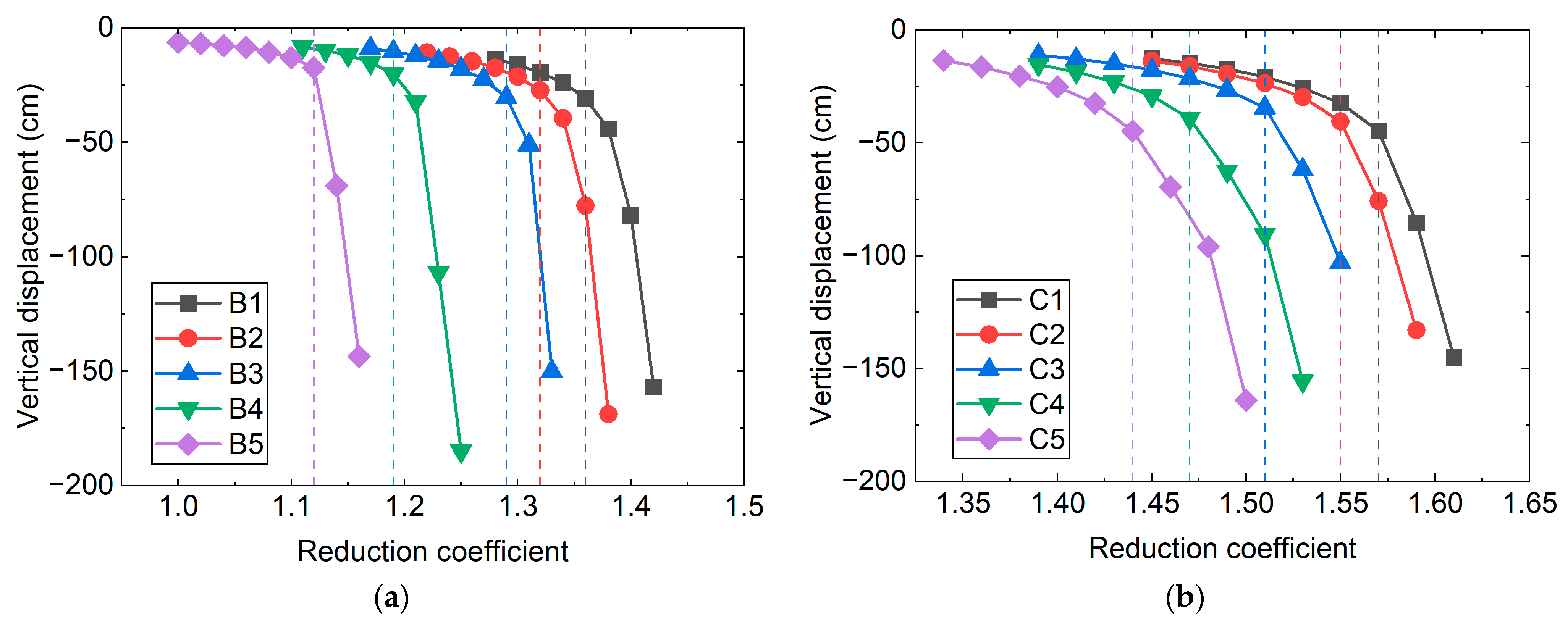
| Method | Stress Release Rate (%) | ||||
|---|---|---|---|---|---|
| 20 | 40 | 60 | 80 | 90 | |
| Three-bench | B1 | B2 | B3 | B4 | B5 |
| CRD | C1 | C2 | C3 | C4 | C5 |
| Variables | Mean | Cov | Probability Distribution Type |
|---|---|---|---|
| Cohesion (kPa) | 10 | 0.2 | Lognormal |
| Friction angle (°) | 30 | 0.1 | Normal |
| Para-Meter | Three-Bench Method | CRD Method | ||||||||
|---|---|---|---|---|---|---|---|---|---|---|
| B1 | B2 | B3 | B4 | B5 | C1 | C2 | C3 | C4 | C5 | |
| C | 32 | 16 | 11.314 | 128 | 45.256 | 22.627 | 5.566 | 16 | 8 | 8 |
| γ | 0.0313 | 0.0442 | 0.063 | 0.008 | 0.0313 | 0.044 | 0.088 | 0.044 | 0.063 | 0.088 |
| Input Random Variable | Cohesion | Friction Angle |
|---|---|---|
| Spearman’s rank correlation coefficient | 0.7741 | 0.5962 |
| Method | 100 Samples (s) | 10,000 Samples (s) | 500,000 Samples (s) |
|---|---|---|---|
| FLAC3D | 345600 | — | — |
| SVR | 0.012 | 0.018 | 0.214 |
Disclaimer/Publisher’s Note: The statements, opinions and data contained in all publications are solely those of the individual author(s) and contributor(s) and not of MDPI and/or the editor(s). MDPI and/or the editor(s) disclaim responsibility for any injury to people or property resulting from any ideas, methods, instructions or products referred to in the content. |
© 2023 by the authors. Licensee MDPI, Basel, Switzerland. This article is an open access article distributed under the terms and conditions of the Creative Commons Attribution (CC BY) license (https://creativecommons.org/licenses/by/4.0/).
Share and Cite
Meng, G.; Li, H.; Wu, B.; Liu, G.; Ye, H.; Zuo, Y. Prediction of the Tunnel Collapse Probability Using SVR-Based Monte Carlo Simulation: A Case Study. Sustainability 2023, 15, 7098. https://doi.org/10.3390/su15097098
Meng G, Li H, Wu B, Liu G, Ye H, Zuo Y. Prediction of the Tunnel Collapse Probability Using SVR-Based Monte Carlo Simulation: A Case Study. Sustainability. 2023; 15(9):7098. https://doi.org/10.3390/su15097098
Chicago/Turabian StyleMeng, Guowang, Hongle Li, Bo Wu, Guangyang Liu, Huazheng Ye, and Yiming Zuo. 2023. "Prediction of the Tunnel Collapse Probability Using SVR-Based Monte Carlo Simulation: A Case Study" Sustainability 15, no. 9: 7098. https://doi.org/10.3390/su15097098
APA StyleMeng, G., Li, H., Wu, B., Liu, G., Ye, H., & Zuo, Y. (2023). Prediction of the Tunnel Collapse Probability Using SVR-Based Monte Carlo Simulation: A Case Study. Sustainability, 15(9), 7098. https://doi.org/10.3390/su15097098