Abstract
This study reflects on the quality aspects of urban meteorological time series obtained by crowdsourcing, specifically the air temperature and humidity data originating from personal weather stations (PWS) and the related implications for empirical and numerical research. A number of year-long hourly-based PWS data were obtained and compared to the data from the authoritative weather stations for selected areas in the city of Vienna, Austria. The results revealed a substantial amount of erroneous occurrences, ranging from singular and sequential data gaps to prevalent faulty signals in the recorded PWS data. These erroneous signals were more prominent in humidity time series data. If not treated correctly, such datasets may be a source of substantial errors that may drive inaccurate inferences from the modelling results and could further critically misinform future mitigation measures aimed at alleviating pressures related to climate change and urbanization.
1. Introduction
In most cities, the existing authoritative observational networks and surveying campaigns are not sufficient in providing comprehensive information on the complex morphologically heterogeneous built environment and the related non-linear developments at the decision scale [1,2]. This is namely due to a low spatial density of individual stations integral to these networks and a limited amount of sensors being installed at these individual monitoring locations. Hence, the resulting low amount of meticulous ground-truth data is severely constraining the collective capacity to properly identify and quantify emerging issues within urban environments [3]. The extensively documented variability of conditions within urban environments further exacerbates the problem [4,5,6,7,8,9]. For instance, it is known that the local atmospheric and ambient conditions may vary within the distance of a couple of streets, which is driven by the unique composition and dynamics of the urban fabric. Specifically, the unique urban composition may induce noticeable differences in air temperature, wind speed, and relative humidity, whereby the unique urban dynamics (e.g., traffic flow and amount of waste heat sources) may affect higher pollutant emissions leading to poor air quality [5,6,7,9]. Wong et al. [5] investigated the street-level microclimate variations in a small urban community in Hong Kong and noted an average variation of air temperature across the street network in the range of 2.2 °C and 2.8 °C for summer and winter, respectively. Jin et al. [9] constructed a detailed spatial map of air pollution concentrations across the city of Bogotá and documented a distinct intra-urban variation within neighbourhoods of each district of the city, where the median PM2.5 yearly concentration level (27.47 μg/m3) at the most polluted district was more than twice the median (13.18 μg/m3) of the least polluted one. Thus, with a limited amount of observational stations and respective in situ data, we cannot obtain a representative construct of environmental conditions within a city. Consequently, current observational records are seen as discontinuous, incomplete, and not comprehensive enough to support enhanced decision-making. This greatly hinders the potential for harnessing these data for optimization and regulation of urban operational functioning, design, and planning in line with the Sustainable Development Goals and the European Green Deal.
At the same time, the past decade has seen a steady increase in crowdsourced data collection practices worldwide. This resulted in the abundant availability of diverse data essential for tackling climate and environmental challenges, which, not surprisingly, has already gained considerable attention in research [10,11,12,13,14]. In general, these data are seen as essential for allowing systematic inference of new knowledge, especially in regions where conventional observations are sparse or completely lacking. Hence, due to the high spatial density of such individual data collection points, we could, in principle, generate a highly needed dataset representative of the urban environment with a high spatial-temporal resolution. Such a dataset would be indispensable to the modelling community as it would provide invaluable means to set up and later evaluate numerical models effectively [15]. For instance, numerical building performance simulations are frequently initiated using standardized weather files that provide an unrealistic portrayal of intra-urban meteorological conditions [16]. Such a practice was proven to be a source of substantial modelling errors that may drive inaccurate inferences from the modelling results [17].
However, it is equally known that the data obtained by crowdsourcing are, in general, less reliable than authoritative observations. They may be prone to errors due to potentially incorrect positioning of the sensors or sporadic sensor’s faulty functioning, which is often not observed nor amended in a timely manner [11,12,14,18,19]. Oftentimes, it may be the case that installed sensors do not abide by the international monitoring procedures and requirements for meteorological instruments, as described by the World Meteorological Organization (WMO) [20]. This may be either due to a lack of knowledge and awareness of these procedures or other constraints, such as a physical lack of space to mount the sensors in an optimal way to eliminate any influencing factors (e.g., artificial waste heat and humidity sources and physical obstructions to the airflow). A number of studies discussed the data quality problematics of crowdsourced data, especially related to the data stemming from personal weather stations (PWS) and offered comprehensive correction methods to amend these issues [11,12,14,18,19,21]. For instance, the work of Nipen et al. [18] discussed the challenges that arise when integrating citizen observations into operational systems, further elaborating robust quality control procedures used to filter out unreliable measurements. Specifically, they elaborated on the spatial test (e.g., “buddy check”, spatial consistency check) that compares lone stations against independent information (e.g., a neighbouring observation) used to validate them. Likewise, Alerskans et al. [21] discussed the specifics of spatial quality control methods and how to optimize them for a more reliable analysis. However, in contrast to the above-mentioned focused discussions and investigations that portray robust data quality methodologies, a bulk of other related work on data quality issues often reflects on aspects that are observed on a level of descriptive statistics (e.g., standard deviation, min-max values, and frequency distribution), while neglecting in-depth observations of the fine-grained temporal evolution of singular or sequential erroneous signals and their implications for empirical and numerical research.
In an effort to address these knowledge gaps, our study aims at answering the following research questions:
- What is the general quality of raw (i.e., unmodified, uncorrected) crowdsourced meteorological data retrieved from the PWS network?
- What is the degree of potential departure of the PWS signal from the authoritative measurements?
- What is the degree of potential deviation between individual neighbouring PWS?
- What are the implications of using the potentially faulty PWS data for empirical and numerical research?
To do so, we obtained a number of year-long hourly-based time series on air temperature and humidity from representative PWS found in close vicinity of in situ authoritative weather stations operated by GeoSphere Austria, the federal institute for geology, geophysics, climatology, and meteorology [22]. Our study further relied on the application of a comprehensive visual analytics tool developed at our institute, which is equipped with tailored dashboards suited for an in-depth structural analysis and quality check of high-dimensional time series data [16,23].
2. Materials and Methods
2.1. Data Acquisition
The hourly-based meteorological data originating from the authoritative observational network and representing the year 2022 are acquired from the open data catalogue managed by GeoSphere Austria [24]. These data depict three morphologically distinct urban locations (Innere Stadt, Hohe Warte, and Donaufeld), as illustrated in Figure 1. These are three out of five urban and peri-urban locations in Vienna that are presently being equipped with monitoring sensors and for which there exist the corresponding PWS data. Many meteorological parameters are monitored at each location; however, we are currently only interested in air temperature and humidity records due to a limited number of parameters measured by the PWS. With respect to the quality aspects, the installation procedure of employed individual semi-automated weather stations strictly follows the WMO standards. The records from these stations are regularly checked for plausibility and completeness, whereby any initial correction takes place in real-time and any implausible values are immediately deleted from the data record [25]. Hence, we can assume these data conform to high-quality standards. To further support this position, all products and services offered by GeoSphere Austria have been officially certificated according to the ISO 9001 standard, which sets out rigorous criteria to ensure high-quality management standards of all related processes and resources [26].
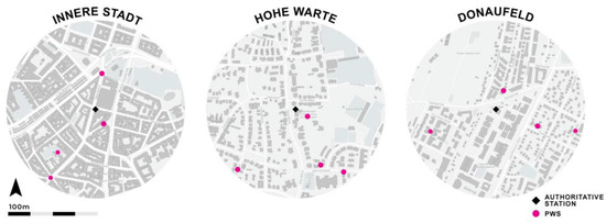
Figure 1.
The selected urban locations in the city of Vienna, Austria, with positions of authoritative (black) and PWS stations (pink). The urban base map was derived from Mapbox maps. We can further observe a highly dense built composition in Innere Stadt, in contrast to the open arrangement of built structures in the other two locations.
The hourly-based crowdsourced data originated from Netatmo’s PWS, a commercially available monitoring system developed for the use of the general public [27]. For the purpose of this paper, we are interested in data originating from Netatmo’s outdoor sensing module capable of measuring air temperature and humidity. Once the module is bought, users may consult the recommendations for the physical installation offered by Netatmo, which stress the importance of abiding by the WMO standards. However, we may assume that it is up to a personal user’s preference if they actually follow such recommendations. Table 1 provides an overview of selected stations along with their descriptive metadata.

Table 1.
The overview of authoritative stations and PWS used for the study.
The general Netatmo data repository may be accessed publicly via an API, and records are freely downloaded and processed for future analysis [28]. Using the available Netatmo Weathermap, we can also visually inspect which data collection points (i.e., PWS) are publicly available for any given location. Once identified, the respective records of these data collection points may be retrieved using their unique stations’ IDs along the individual sensing module ID, whereby the desired data resolution, data parameter, and a specified timeframe should also be provided. The response is provided in a json format, which can be further processed with a number of applications. We have used Microsoft Excel software (version 2016 64-Bit Edition) to bring the data in a format compatible with the visual analytics tool used for data structure and quality assessment.
2.2. Towards a Comparative Analysis
For each of the three stations from the authoritative observational network, we have selected four corresponding PWS that further conform to the principles of the well-established Local Climate Zone (LCZ) classification system [29,30]. Specifically, the LCZ classification system denotes 17 distinct regions with relatively homogeneous surface cover, structure, material, and human activity, where characteristic atmospheric conditions (for that particular LCZ class) may be expected within a radius between 200 to 500 m. Hence, using the respective authoritative station as an epicentre, we have selected four complementary PWS falling within the 400 m radius. Figure 1 illustrates the spatial positioning of selected authoritative and PWS stations. To further identify which location is representative of which LCZ class, we have used the freely available global map of Local Climate Zones that provides standardized and harmonized data of all cities while capturing the intra-urban heterogeneity across the whole surface of the earth [31]. The global LCZ map was clipped for the selected locations to derive the spatial distribution of corresponding LCZ classes within the targeted radius of 400 m. We have observed a predominantly uniform allocation of specific LCZ classes across the respective locations, ranging from highly dense (LCZ 2) for Innere Stadt to a rather open arrangement of built structures (LCZ 6 and 8) for Hohe Warte and Donaufeld locations (Figure 2).
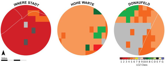
Figure 2.
The spatial distribution of respective LZC classes for the selected urban locations in the city of Vienna, Austria, is derived from the global LCZ map, which is offered under the Creative Commons Attribution 4.0 International license [29].
The conceptualization of employed comparative analysis of the acquired authoritative and PWS meteorological data was based on well-established spatial methods that focus on the detection of inconsistencies between neighbouring stations [18,19,32]. This method is often dubbed a “buddy check”, which denotes a comparison of an observed value (in this case, a respective PWS data point) against another “buddy” observation (in this case, a respective data point from an authoritative observation) that is within a 3 km radius and have elevations within 30 m [18]. The process implies that an observation is removed if its deviation from the average is more than twice the standard deviation of the observations in the neighbourhood. This is especially fitting for use cases that tackle the same atmospheric phenomena. Further complying with the LCZ classification system, the selected radius of 400 m in this study is expected to derive a finer comparison.
It should be further noted that, in contrast to the existing vast scientific body of work that thoroughly covers methodologies for quality control of meteorological data, as noted at the outset, in our work, we aimed to highlight quality issues that are integral to the crowdsourced PWS data and the resulting implications that arise when such data is used for empirical research and numerical simulation, specifically when data quality issues are not being resolved. We have also noted that related work oftentimes does not focus on all nuances of data quality issues. Hence, our intention here is to deepen the discussion in this regard.
2.3. Data Exploration
Data exploration was carried out using a visual analytics (VA) system developed at our institution [16,20]. The system offers meticulously designed analytics dashboards for an in-depth structural analysis and quality check of time series data. For instance, we may inspect the completeness of time series data (i.e., detection of missing values and missing periods), the accuracy of time series data (i.e., detection of duplicate timestamps), or carry out an anomaly detection (i.e., detection of outliers or unusual sequences of identical values). These insights are offered within a composite tabular visualization further enriched with the frequency of singular events (0–100%) and temporal distribution with monthly and yearly allocation and spatial positioning (i.e., when in time did a particular event occurred), as seen in Figure 3. To allow for intelligent visual identification of potential missing values, the respective temporal gaps are highlighted directly within the line plot depicting a temporal distribution of a selected time series. The alternative stacked visualization of selected time series may be further used for an intra-comparison of temporal discrepancies of different time series.
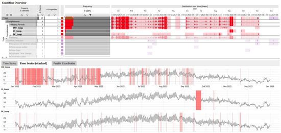
Figure 3.
Visual analytics dashboard for an in-depth exploration of data quality metrics: (1) tabular visualization of various completeness and accuracy metrics (top); (2) stacked line plots representing the temporal distribution of sampled time series with detected temporal gaps depicted in red (bottom).
3. Results
3.1. On the Quality of Raw PWS Data
Once the acquired raw time series data were inspected visually using the VA system, the identification of existing inconsistencies was instantaneous. It should be noted that here, we are presenting the temperature time series only, as both meteorological parameters are measured by the same sensing module; hence their recording cycles would be the same. A comparative assessment of all PWS data streams revealed that many PWS show a discrepancy in length relative to the corresponding authoritative observations (Figure 4). In some cases, this discrepancy was more prominent, such as in the case of stations HW_03 and DF_02 (Figure 4). This indicates that there are a number of time gaps which are not taken into account while retrieving the data from the Netatmo data repository. Namely, once the data is retrieved from the respective data repository, the dataset is provided as a continuous sequence of data points where any potential gaps are omitted by providing such a “compressed” dataset. Furthermore, there is no indication of the actual temporal placement of integral time gaps nor the frequency of their occurrence, which results in notable misalignment in the temporal distribution of records when compared to the corresponding authoritative observations (Figure 5). Oftentimes it would appear as if there were inversed trends and inconsistencies in peak values, which would significantly impact any inferences drawn from such data. We may further observe the irregularities in the amount of gaps present in each of the PWS datasets (Figure 4). This is mostly dependent on the individual running procedures of the PWS and the potential defects in running regimes. Thus, the integrity of any future investigation relying on the PWS data would also be highly dependent on the choice of the PWS used for the purpose.
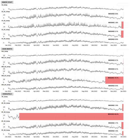
Figure 4.
A comparative visual assessment of the quality of the raw temperature time series datasets originating from the PWS and the respective authoritative observations over three urban locations: Innere Stadt (top), Hohe Warte (middle), Donaufled (bottom). The respective authoritative observations are shown as the first liner plot in all individual graphs. The respective discrepancy in length observed for the PWS time series is marked in red.
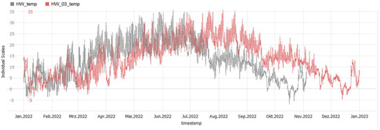
Figure 5.
A portrayal of a temporal misalignment of temperature records and the noted inversed trends between the selected PWS (in red) and the respective authoritative station (in grey).
3.2. On the Discrepancies between PWS and Authoritative Data
In the following step, all PWS data was corrected in order to account for the existing time gaps. We may now visually inspect all the individual occurrences of respective gaps, whereby there seems to be no particular regularity or periodicity in their manifestation across different PWS (Figure 6, Figure 7 and Figure 8). As noted previously, this is mostly due to the individual running regimes of each PWS. As these devices are essentially wireless and hence, their functioning is dependent on the established Wi-Fi connection; any alteration in this connection would result in an interruption of operation. In some instances, these gaps appear to be minor; thus, a reconstruction by interpolation or other methods may be possible. However, in other cases, the gaps are in order from one week to a couple of consecutive weeks, which makes the data reconstruction unfeasible. One specific case is the PWS DF_02 from location Donaufeld (Figure 8), where the station seems to be installed at the beginning of December 2022; hence such data would be unusable for any pertinent exploration.
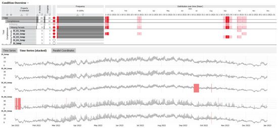
Figure 6.
An overview of corrected PWS data for location Innere Stadt depicting the actual placement of temporal gaps (bottom), along with completeness metrics (top).
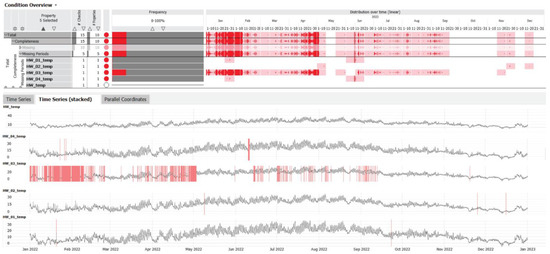
Figure 7.
An overview of corrected PWS data for location Hohe Warte depicting the actual placement of temporal gaps (bottom), along with completeness metrics (top).
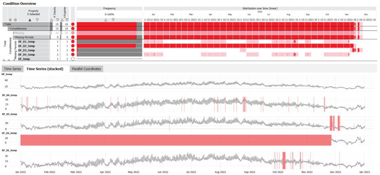
Figure 8.
An overview of corrected PWS data for location Donaufeld depicting the actual placement of temporal gaps (bottom), along with completeness metrics (top).
To allow for a deeper inspection of the PWS time series, we derived respective deviations from the corresponding authoritative time series, where the authoritative time series is observed as a baseline. Hence, whenever a computed deviation equals a positive value, the observed PWS signal is higher than its corresponding authoritative time series and vice versa. The respective equation is as follows:
where ∆pi denotes a deviation of a concerned meteorological parameter, in this case, temperature or humidity, for the time step i, and pPWSi and pAOi denote PWS and authoritative records for the same time step i, respectively.
∆pi = pPWSi − pAOi,
Looking at the computed deviations, we can observe the tendency towards both the overestimation and the underestimation of recorded PWS values for temperature and humidity records (Figure 9, Figure 10 and Figure 11). For temperature data, the maximum positive deviation was 25 °C, and the maximum negative deviation was −11.5 °C across all the PWS for all three locations. For humidity data, the maximum positive deviation was 59%, and the maximum negative deviation was −39%. In general, we cannot observe a particular regularity in regard to the temporal distribution of such events, as the existing deviations appear to be equally spread out over the entire year. However, there may be an indication of a possible tendency towards more pronounced deviations during warmer months, which is more distinct in the case of temperature time series.
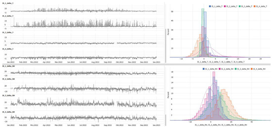
Figure 9.
Temporal distribution of computed deviations for temperature (top) and humidity (bottom) for location Innere Stadt: respective time series are given on the (left) side of the figure, and the frequency of event distribution is given on the (right) side of the figure.
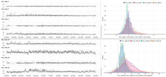
Figure 10.
Temporal distribution of computed deviations for temperature (top) and humidity (bottom) for location Hohe Warte: respective time series are given on the (left) side of the figure, and the frequency of event distribution is given on the (right) side of the figure.
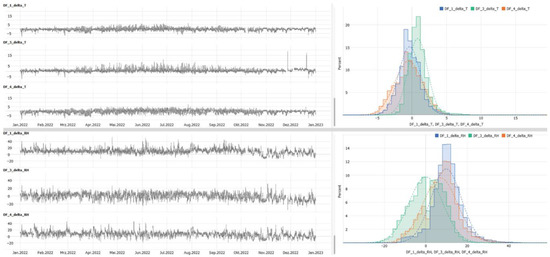
Figure 11.
Temporal distribution of computed deviations for temperature (top) and humidity (bottom) for location Donaufled: respective time series are given on the (left) side of the figure, and the frequency of event distribution is given on the (right) side of the figure.
However, it should be noted that this particular assessment relied on the authoritative data sources being taken as the absolute possible truth in terms of quality standards. Such a position resulted from the previously discussed rigorous data quality control procedures employed at GeoSphere Austria, further reinforced by the ISO 9001 certification. However, in order to conform to the scope of scientific objectivity, we would like to propose a possibility that there may still be a certain level of uncertainty (i.e., the “error bar”) attributed to the authoritative data, which has not been accounted for in this study.
Looking at the frequency of all deviation events in temperature time series (see histogram plots in Figure 9, Figure 10 and Figure 11), deviations between −5 °C to 5 °C are very prominent, with observed left-skewed distribution denoting a general tendency towards overestimation of values. Furthermore, we can observe an uneven development of deviations across individual PWS. This is especially evident in the case of PWS IS_02, where the overestimation of values reaches 25 °C. In the case of humidity data, a strong shift towards the generally higher values is even more evident across all PWS, which is particularly pronounced in location Hohe Warte for PWS HW_02 (Figure 10). Some exemptions to this case are observed for PWS IS_02 and DF_03, where the extent of values goes over the negative range denoting the underestimation of records. In addition, we may observe the highest clustering of deviations in the range of 0% to 20% for humidity values.
3.3. On the Discrepancies between the Neighbouring PWS Data
Looking at the individual PWS time series and how they correlate to one another, we may observe notable discrepancies in the case of both temperature and humidity values (Figure 12 and Figure 13). Although the distinct temporal distribution curves across all time series appear to conform to an overall comparable progression (see Figure 6, Figure 7 and Figure 8), a myriad of individual time-based events significantly deviate from this progression. In regard to the temperature time series, such a departure is the most evident for the PWS originating from the location Innere Stadt (Figure 12). Namely, one pronounced outlier is the PWS IS_02 where the temperature values appear to be generally higher than for the remaining neighbouring PWS. This can be observed in the boxplot in Figure 12 but also in the complementary frequency plot where the normal distribution of IS_02 data denotes a flatter curve with a prominent shift towards a higher range. We can also observe rather unrealistic values recorded at IS_02, where the temperature maximum reaches 50 °C. Furthermore, at the location Donaufeld, a slight shift in the normal distribution for PWS DF_03 in relation to the other neighbouring PWS may be observed, whereby DF_01 and DF_04 appear to correspond well to one another. It should be noted that we took into account only the complete records of three PWS from Donaufeld for this investigation and excluded the PWS DF_02, for which there is only one month of data. The temperature records for PWS in the location Hohe Warte appear to correlate the most with one another.
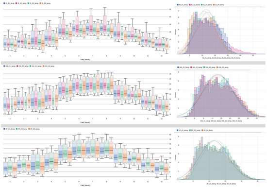
Figure 12.
Monthly distribution of temperature data spread across neighbouring PWS and their respective locations: a combined comparison of data distribution using the boxplot visualization (left), along with the frequency of event distribution (right).
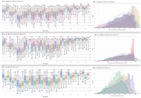
Figure 13.
Monthly distribution of humidity data spread across neighbouring PWS and their respective locations: a combined comparison of data distribution using the boxplot visualization (left), along with the frequency of event distribution (right).
The visual analysis of the humidity data revealed even more pronounced discrepancies across all time-series and locations (Figure 13). As noted above, the general temporal progression appears to be consistent across time series (see Figure 6, Figure 7 and Figure 8); however, a clear misalignment of normal distribution curves is observed as a common trait. This may indicate either a relative shift towards a higher or a lower range (see frequency plot in Figure 13). If we look at the records from PWS IS_02, for example, in contrast to the above observations, it appears that there is a prominent spread over a lower range in the case of humidity data. This namely means that the temperature sensor in PWS IS_02 tends to overestimate, whereby the humidity sensor may be more inclined towards underestimation of recorded values relative to the other neighbouring PWS. The highest shift in the normal distribution relative to the neighbouring PWS is observed for PWS originating from location Donaufeld. In general, in the case of humidity data a significant offset between individual PWS is quite prominent, which diverges from the temperature observations where the records were found to correlate well. The same may be concluded for PWS at locations Hohe Warte. Hence, we again observed a conflicting temporal behaviour of data recorded by temperature and humidity sensors stemming from the same module.
4. Discussion
4.1. Summarized Observations
When analysing the raw PWS data, we observed a notable discrepancy in length for the retrieved time series data relative to their corresponding authoritative time series. This denotes a critical issue of potential oversight of existing data gaps if not amended prior to any further analysis. As these time series are retrieved as a “compressed” sequence of data points with no temporal indication of such integral data gaps, the resulting misalignment with the reference data, in our case, the authoritative observations, is an unavoidable consequence and, hence, has to be properly regarded.
Once the data were corrected for the above-mentioned inaccuracies, we investigated the apparent departure of PWS data from the corresponding authoritative observations. Our analysis revealed a substantial amount of erroneous occurrences, ranging from singular to sequential events. Namely, a prevailing tendency towards both the overestimation and the underestimation of data was observed, with a noticeable variability in their distribution. However, a general tendency towards higher values in PWS was recurrent in all locations, whereby such a tendency was particularly visible for the humidity time series.
There are equally notable discrepancies between the neighbouring PWS time series and the data retrieved from different points within the same urban domain. Although a comparable progression of distribution curves was observed, we could not establish a particular rule for the apparent faulty signals. Nevertheless, for both temperature and humidity data, a noteworthy misalignment of individual frequency distribution curves are observed in respect to both the shape and the positioning of the curve. This suggests either a relative shift towards a higher or a lower range, thus denoting either an overestimation or underestimation of values. In some instances, given the potential clustering of some PWS curves, we could indicate whether there is a shift to the lower or a higher range. Regardless of the specifics about the nature of the departure, the critical remark is that there is a significant departure, which denotes conflicting information stemming from the PWS modules.
4.2. Comparison over Multiple Years
In order to validate that the above-summarized observations are not the isolated instance that may be solely attributed to a certain year, a multiannual analysis over 4 years has been carried out. Figure 14 illustrates an exemplary case that focuses on the temporal distribution of temperature data for a selected PWS (IS_03) within the location Innere Stadt. First, the case of data gaps may be observed for each year with their temporal placement following a rather irregular behaviour. Second, the amount of respective data gaps and their sequential duration differs from year to year. Lastly, looking at the computed deviations, further irregularities may be observed in terms of their intensity and variability. In conclusion, the data quality notions discussed in this paper should not be attributed to a single year, rather, they are of a much broader character.

Figure 14.
Multiannual temporal distribution of temperature data for the location Innere Stadt illustrations a selected PWS (IS_03) against respective authoritative observations (middle) and computed deviations (bottom), along with a tabular visualization of completeness metrics (top).
4.3. On the Implications of Using Faulty PWS Data for Empirical Research and Numerical Simulation
Given the above discussion, it is sensible to allude to a number of related implications when using potentially faulty PWS data for empirical research and numerical simulation. First, if no attention were given to data quality assessment, we would not only rely on incomplete raw data but also on integral conflicting trends and temporal developments (relative to the authoritative observations), which would insinuate unrealistic seasonal and diurnal progressions of concerned meteorological parameters. Second, as the corrected progression of PWS data still unveiled a fluctuating alignment to the authoritative observations, this further indicates possible future implications for simulation-supported system performance assessments when such data would be used as external boundary conditions. Specifically, this would result in potential oversizing or under-sizing of internal systems, such as the HVAC systems in building structures, or poor estimation of indoor building heating and cooling regimes. Furthermore, implications are equally critical for empirical research as the faulty meteorological characteristics would critically misinform future mitigation measures aimed at alleviating pressures related to climate change and urbanization. Lastly, given a considerable degree of variation in the distribution of meteorological parameters between individual PWS stemming from the same location, selecting a representative weather station with the most realistic data poses yet another level of concern.
4.4. Replication Potential to Other Cities
Due to the vast international geospatial coverage of the Netatmo PWS network, the replication potential of the introduced assessment methodology is generally large. However, one factor limiting direct transferability may be the unavailability of the authoritative data sources at chosen localities. This especially concerns data-sparse geographical regions, such as the Southern Hemisphere, as highlighted in the data gap report drafted by the ConnectinGEO project that looked at the existing data gaps in European in situ Earth Observation networks [33]. Led by these dire information needs, European Commission had set itself on a path to remedy these constraints for future applications through a widespread initiative for greater availability of qualitative and quantitative in situ environmental data contributing to the in situ component of existing observation systems. However, as this is still an ongoing and time-intensive process, the replication potential of the introduced assessment methodology in current data-sparse regions remains limited for the time being.
4.5. Future Prospects for Correcting Faulty Data
In our current application, we have employed a number of measures to assess the data quality of PWS time series data in an effort to determine the degree to which these data are accurate, complete, and consistent. Specifically, we performed a completeness check (i.e., detection of missing and incomplete data values), consistency check (i.e., checking for any sudden or unexpected changes in the data by comparing the data with external sources), outlier check (i.e., detection of values well above or below a certain threshold), and we have inspected the data for tendencies and trends. These checks were supported by a dedicated visualization system that helped us carry out a visual detection of existing faulty signals in selected PWS time series.
Once these faulty signals are identified, the following step would be to create a reasonably accurate dataset where any unreliable data points are removed. One possibility would be to apply a “buddy check” approach [18], which has been discussed in Section 2.2. The process implies that a data point is removed if its deviation from the average is more than twice the standard deviation of the observations in the neighbourhood. To test this approach, we have computed the respective deviations for each PWS and their neighbouring authoritative stations, whereby these were computed on a daily basis. Specifically, for each day, each hourly data point in the PWS time series was compared to the respective average over the entire day, and this difference was further compared to the doubled standard deviation of the neighbouring authoritative station computed on the same daily basis. Figure 15 illustrates the resulting tolerance violation, specifically the visualization of those instances where the threshold with respect to the standard deviation is breached for all PWS stations. These violations are visualized every 10 days of a month, whereby light orange rectangles in Figure 15 denote the presence of a tolerance violation for that 10-day window, and darker orange lines denote the amount of individual tolerance violations per day. Table 2 provides an overview of the total number of violation instances for each PWS and their respective parameters. Such computations are expected to help us confirm or reject a particular observation and derive a more reliable dataset for future applications.
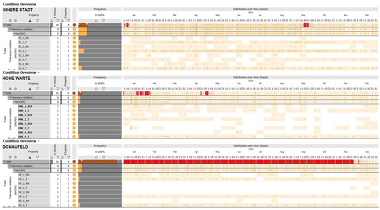
Figure 15.
Tolerance violation for PWS time series data: Innere Stadt (top); Hohe Warte (middle); Donaufled (bottom).
Table 2.
The overview of the total number of violation instances for PWS used for the study.
5. Conclusions
This contribution addressed a number of issues indicating the importance of data quality assessment of crowdsourced meteorological data. For the purpose of our study, we used year-long temperature and humidity data retrieved from Netatmo’s personal weather stations network from selected urban locations in the city of Vienna, Austria, and further compared these to the in situ authoritative observations. We first explored raw PWS data, which have not been corrected for any potential deficiencies, and noted some critical aspects related to the integral data gaps. However, even when corrected for these gaps, the PWS data still displayed a prominent departure from in situ authoritative observations expressed as overestimation or underestimation of hourly-based records. The degree of such departure varied across the study PWS but was nevertheless evident. Hence, we also looked at the individual profiles of neighbouring PWS and noted a significant misalignment, with a relative shift towards a higher or a lower range denoting either an overestimation or underestimation of values. In summary, our investigation revealed a substantial amount of erroneous occurrences, ranging from singular to sequential events. Such occurrences were equally present over multiple years, stressing the fact that data quality issues should not be attributed to a single year, rather they are of a much broader character. Consequently, if not treated in a timely manner, such erroneous occurrences would introduce a significant bias in inferences drawn from such data and further affect future empirical and numerical applications relying on these data.
However, it should be noted that there may be some limitations to our study to which we aim to raise attention. First, the fact that the authoritative observations have been taken as the absolute truth in terms of quality standards may raise questions regarding scientific objectivity. Even if tangible arguments supporting such a position exist, we acknowledge that the observations made by authoritative stations could still have biases of their own. However, as the information about an actual possible estimated error bar for the authoritative data is not known at this time, these aspects are not addressed in this study. Second, even if the spatial distribution of PWS is generally large, the replication potential of the discussed methodology may be affected by the unavailability of supporting authoritative data sources at chosen localities.
Author Contributions
Conceptualization, M.V.; methodology, M.V.; software, J.S.; validation, M.V. and J.S.; formal analysis, M.V.; investigation, M.V.; resources, M.V.; data curation, M.V.; writing—original draft preparation, M.V.; writing—review and editing, M.V. and J.S.; visualization, M.V.; supervision, J.S.; project administration, J.S.; funding acquisition, J.S. All authors have read and agreed to the published version of the manuscript.
Funding
VRVis is funded by BMK, BMDW, Styria, SFG, Tyrol, and Vienna Business Agency in the scope of COMET—Competence Centers for Excellent Technologies (879730), which is managed by FFG.
Institutional Review Board Statement
Not applicable.
Informed Consent Statement
Not applicable.
Data Availability Statement
Meteorological data from authoritative observations may be accessed from here: https://data.hub.zamg.ac.at/ (accessed on 16 January 2023). Meteorological data from the Netatmo PWS network may be accessed from here: https://dev.netatmo.com/apidocumentation/weather (accessed on 16 January 2023) [28].
Conflicts of Interest
The authors declare no conflict of interest.
References
- Hamdi, R.; Kusaka, H.; Doan, Q.-V.; Cai, P.; He, H.; Luo, G.; Kuang, W.; Caluwaerts, S.; Duchêne, F.; Van Schaeybroek, B.; et al. The State-of-the-Art of Urban Climate Change Modeling and Observations. Earth Syst. Environ. 2020, 4, 631–646. [Google Scholar] [CrossRef]
- Muller, C.; Chapman, L.; Grimmond, C.S.B.; Young, D.; Cai, X. Sensors and the city: A review of urban meteorological networks. Int. J. Climatol. 2013, 33, 1585–1600. [Google Scholar] [CrossRef]
- Marsh, A.S.; Negra, C.; O’Malley, R. Closing the Environmental Data Gap. Issues Sci. Technol. 2009, 25, 69–74. [Google Scholar]
- Masson, V.; Lemonsu, A.; Hidalgo, J.; Voogt, J. Urban Climates and Climate Change. Annu. Rev. Environ. Resour. 2020, 45, 411–444. [Google Scholar] [CrossRef]
- Wong, P.P.Y.; Lai, P.-C.; Hart, M. Microclimate Variation of Urban Heat in a Small Community. Procedia Environ. Sci. 2016, 36, 180–183. [Google Scholar] [CrossRef]
- Kousis, I.; Pigliautile, I.; Pisello, A.L. Intra-urban microclimate investigation in urban heat island through a novel mobile monitoring system. Sci. Rep. 2021, 11, 9732. [Google Scholar] [CrossRef]
- Vuckovic, M.; Kiesel, K.; Mahdavi, A. The Extent and Implications of the Microclimatic Conditions in the Urban Environment: A Vienna Case Study. Sustainability 2017, 9, 177. [Google Scholar] [CrossRef]
- Vuckovic, M.; Kiesel, K.; Mahdavi, A. Studies in the assessment of vegetation impact in the urban context. Energy Build. 2017, 145, 331–341. [Google Scholar] [CrossRef]
- Jin, Z.; Andrés, V.A.M.; Ivan, M.; Felipe, F.J. Enriched spatial analysis of air pollution: Application to the city of Bogotá, Colombia. Front. Environ. Sci. 2022, 10, 1777. [Google Scholar] [CrossRef]
- See, L. A Review of Citizen Science and Crowdsourcing in Applications of Pluvial Flooding. Front. Earth Sci. 2019, 7, 44. [Google Scholar] [CrossRef]
- Droste, A.M.; Heusinkveld, B.G.; Fenner, D.; Steeneveld, G.-J. Assessing the potential and application of crowdsourced urban wind data. Q. J. R. Meteorol. Soc. 2020, 146, 2671–2688. [Google Scholar] [CrossRef]
- Fenner, D.; Bechtel, B.; Demuzere, M.; Kittner, J.; Meier, F. CrowdQC+—A Quality-Control for Crowdsourced Air-Temperature Observations Enabling World-Wide Urban Climate Applications. Front. Environ. Sci. 2021, 9, 553. [Google Scholar] [CrossRef]
- Potgieter, J.; Nazarian, N.; Lipson, M.J.; Hart, M.A.; Ulpiani, G.; Morrison, W.; Benjamin, K. Combining High-Resolution Land Use Data with Crowdsourced Air Temperature to Investigate Intra-Urban Microclimate. Front. Environ. Sci. 2021, 9, 385. [Google Scholar] [CrossRef]
- Bárdossy, A.; Seidel, J.; El Hachem, A. The use of personal weather station observations to improve precipitation estimation and interpolation. Hydrol. Earth Syst. Sci. 2021, 25, 583–601. [Google Scholar] [CrossRef]
- Best, M.J. Progress towards better weather forecasts for city dwellers: From short range to climate change. Theor. Appl. Climatol. 2006, 84, 47–55. [Google Scholar] [CrossRef]
- Vuckovic, M.; Schmidt, J. Visual Analytics Approach to Comprehensive Meteorological Time-Series Analysis. Data 2020, 5, 94. [Google Scholar] [CrossRef]
- Vuckovic, M.; Hammerberg, K.; Mahdavi, A. Urban weather modeling applications: A Vienna case study. Build. Simul. 2020, 13, 99–111. [Google Scholar] [CrossRef]
- Nipen, T.N.; Seierstad, I.A.; Lussana, C.; Kristiansen, J.; Hov, Ø. Adopting citizen observations in operational weather prediction. Bull. Am. Meteorol. Soc. 2020, 101, 43–57. [Google Scholar] [CrossRef]
- Sgoff, C.; Acevedo, W.; Paschalidi, Z.; Ulbrich, S.; Bauernschubert, E.; Kratzsch, T.; Potthast, R. Assimilation of crowd-sourced surface observations over Germany in a regional weather prediction system. Q. J. R. Meteorol. Soc. 2022, 148, 1752–1767. [Google Scholar] [CrossRef]
- World Meteorological Organization. Guide to Meteorological Instruments and Methods of Observation, oCLC: 288915903; World Meteorological Organization: Geneva, Switzerland, 2008. [Google Scholar]
- Alerskans, E.; Lussana, C.; Nipen, T.N.; Seierstad, I.A. Optimizing Spatial Quality Control for a Dense Network of Meteorological Stations. J. Atmos. Ocean. Technol. 2022, 39, 973–984. [Google Scholar] [CrossRef]
- GeoSphere Austria. 2023. Available online: https://www.geosphere.at/ (accessed on 16 January 2023).
- Vuckovic, M.; Schmidt, J. Visual Analytics for Climate Change Detection in Meteorological Time-Series. Forecasting 2021, 3, 276–289. [Google Scholar] [CrossRef]
- GeoSphere Austria Data Hub. 2023. Available online: https://data.hub.zamg.ac.at/ (accessed on 16 January 2023).
- GeoSphere Austria. Data Validation. 2023. Available online: https://www.zamg.ac.at/cms/de/klima/messnetze/datenpruefung (accessed on 16 January 2023).
- GeoSphere Austria, ISO 9001. 2023. Available online: https://www.zamg.ac.at/cms/en/topmenu/about-us/quality-management (accessed on 24 March 2023).
- Netatmo. 2023. Available online: https://www.netatmo.com/en-us (accessed on 16 January 2023).
- Netatmo Connect. 2023. Available online: https://dev.netatmo.com/apidocumentation/weather (accessed on 16 January 2023).
- Stewart, I.D.; Oke, T.R. Local Climate Zones for Urban Temperature Studies. Bull. Am. Meteorol. Soc. 2012, 93, 1879–1900. [Google Scholar] [CrossRef]
- Demuzere, M.; Hankey, S.; Mills, G.; Zhang, W.; Lu, T.; Bechtel, B. Combining expert and crowd-sourced training data to map urban form and functions for the continental US. Sci. Data 2020, 7, 264. [Google Scholar] [CrossRef] [PubMed]
- Demuzere, M.; Kittner, J.; Martilli, A.; Mills, G.; Moede, C.; Stewart, I.D.; van Vliet, J.; Bechtel, B. A global map of local climate zones to support earth system modelling and urban-scale environmental science. Earth Syst. Sci. Data 2022, 14, 3835–3873. [Google Scholar] [CrossRef]
- Fiebrich, C.A.; Morgan, C.R.; McCombs, A.G.; Hall, P.K.; McPherson, R.A. Quality Assurance Procedures for Mesoscale Meteorological Data. J. Atmos. Ocean. Technol. 2010, 27, 1565–1582. [Google Scholar] [CrossRef]
- ConnectinGEO. 2023. Available online: http://www.connectingeo.net (accessed on 24 March 2023).
Disclaimer/Publisher’s Note: The statements, opinions and data contained in all publications are solely those of the individual author(s) and contributor(s) and not of MDPI and/or the editor(s). MDPI and/or the editor(s) disclaim responsibility for any injury to people or property resulting from any ideas, methods, instructions or products referred to in the content. |
© 2023 by the authors. Licensee MDPI, Basel, Switzerland. This article is an open access article distributed under the terms and conditions of the Creative Commons Attribution (CC BY) license (https://creativecommons.org/licenses/by/4.0/).