Peaking Dynamics of the Production Cycle of a Nonrenewable Resource

Abstract

We use a system dynamics model to analyse the cycle of production of a nonrenewable natural resource, with a specific interest in crude oil. This subject has been empirically studied for a long time. However, modelling studies able to correlate the peaking with the parameters of the system have been very rare, and only recently proposed. In the present paper, we examine the timing of the peaking mainly as a function of the energy return for energy invested (EROI). The model provides approximate formulas for evaluating the peak time and “rules of thumb” that are useful for understanding the peaking phenomenon in the exploitation of natural resources. It shows that the peaking of the production curve occurs at a time that is inversely proportional to the EROI of the process at the start of the cycle.

1. Introduction

The idea that the production of a nonrenewable resource follows a “bell-shaped” curve was first proposed by Marion King Hubbert in 1956 for crude oil in the continental United States [1]. The term “peak oil” became fashionable in the early 2000s to indicate the peak of the global oil production curve. The mainstream debate lost interest in the concept of peak oil when some of the early predictions of the peak date turned out to have been misplaced [2].

Bell-shaped curves were later observed for crude oil in several productive regions [3], and the same kind of curve was observed for other fossil fuels (e.g., coal), for mineral resources [4], and for theoretically renewable resources that were exploited faster than they could re-form by natural processes (for instance, whale oil) [5,6,7].

In qualitative terms, the bell-shaped curve is easily understandable considering the differential costs of the extraction (or production) of a nonrenewable resource. Because the cheaper resources are produced first, the cost or production tend to gradually increase, reducing profits. The consequence is a reduction in investments that generates a decline in production. Hence, peaking necessarily appears at some moment.

The concept of peak oil generated a widespread debate, with some authors discounting it as an arbitrary concept [7], while, for others, it represented a watershed that would lead to profound changes in human civilization [8]. Given this attitude, it was believed that determining the peak date in advance was of the utmost importance. Various approaches were used for this purpose, mainly based on fitting the historical data with various mathematical curves [9] or using such methods as “Hubbert Linearization” [10]. These approaches were found to be inaccurate, and the mainstream debate lost interest in peak oil when some of the early predictions of the peak date turned out to have been misplaced [11].

In time, some models based on system dynamics were proposed for the production cycle [2,12,13]. These models are based on measurable parameters, and particularly the one called “Energy Return for Energy Invested” (EROI or EROEI) [14]. The EROI is the ratio of the energy produced by a plant or system over its lifetime to the energy needed to build, supply, maintain, and eventually dismantle the producing plant(s).

The EROI of crude oil has been discussed in depth by Hall, Murphy, and coworkers [8,9,10]. They show the gradual reduction in the EROI of crude oil production as extraction has proceeded over the past decades. It is this reduction that reduces monetary profits and causes a decline in investments.

Nevertheless, these models lacked the capability to determine a fundamental element of the system, the one that had been the objective of many past studies: the timing of the production peak. Therefore, in the present paper, we develop an approximate solution of the differential equations of the resource extraction model, and we use it to determine how the EROI and other parameters affect the timing of the peak. The main result is that the time to peak for a nonrenewable resource extracted in free-market conditions is inversely proportional to the value of the EROI at the start of the production cycle. We apply this model to a real-world “toy system” that shows the main elements of the dynamical model [11].

This study may be used as an alternative method to the empirical ones to estimate the peaking data of a real-world system, but we believe that its main value is to provide a better understanding of the peaking phenomenon in terms of its causes and the parameters that influence it.

2. Methods

The term “complex systems” refers to systems out of thermodynamic equilibrium, typically described as “complex adaptative systems” (CASs) [12] when they are dominated by feedback effects. These systems can be modelled using the technique called “system dynamics” [13], where the elements of the systems under study are described in terms of “stocks” or “levels” linked to each other by “flows” of matter, energy, or other entities. When a flow rate depends on the size of a stock that it connects to, the resulting interaction is called “feedback.” Typically, CASs tend to attain a steady-state condition, defined as homeostasis (or “homeorhesis” when the system oscillates around a fixed set of parameters).

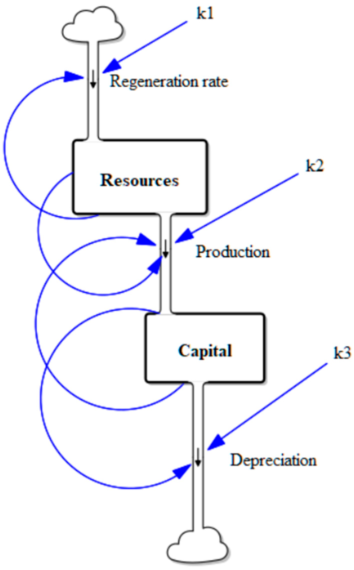
The system dynamics approach can be applied to model the production of a nonrenewable resource, such as crude oil, by the following assumptions:

• The resource is defined as an initial fixed stock. In the case of crude oil, it is the ensemble of the extractable resources (“URR” (ultimate recoverable resources));
• The extraction and processing of the resource transform it into a stock called “capital” that aggregates all the economic entities created by the process. The flow from the resource stock to the capital stock is called “production”;
• The resource stock is depleted proportionally to the size of the capital stock;
• The capital stock grows in proportion to the amount of the remaining resources, and to the amount of available capital;
• The capital stock is depleted at a rate proportional to the size of the stock (“depreciation”).

These assumptions can be quantified using system dynamics. In developing the model, we chose the simplest possible assumptions: we assumed that the flows are linearly proportional to the stocks they are connected to, and that there are no other factors affecting them. Other assumptions are possible, but we found that the ones we chose generate a model that is able to reproduce the data from historical cases in a quantitative manner [6,14]. The model is shown in Figure 1, using the graphic conventions of system dynamics (that is, with stocks drawn as boxes and flows as arrows). Note how the model is drawn in such a way as to emphasize that the flows have a “downward” direction, in analogy with the flow of a liquid in a gravitational field. This is just a graphic convention; it does not affect the model itself. Note that the model shown in the figure assumes the possibility of a regeneration of the resource stock, but this does not occur for nonrenewable resources.

The equations underlying the graphic representation of Figure 1 are shown below. We term the two stocks as “Resources” and “Capital” (R and C), and we label the flow constants as kn.

dR/dt = k₁R − k₂RC

(1)

dC/dt = ηk₂RC − k₃C

(2)

In the equations, η (eta) is the efficiency of the transformation of the resource into useful energy to be accumulated in the capital stock. It is a dimensionless number that can go from 0 to 1 if the two stocks are measured using the same units. As written, the model is equivalent to the Lotka–Volterra one [15]. If, instead, the resource is not renewable, then we can assume that k₁ = 0, and the first equations (Equations (1)) of the system become as follows:

dR/dt = −k₂RC

(3)

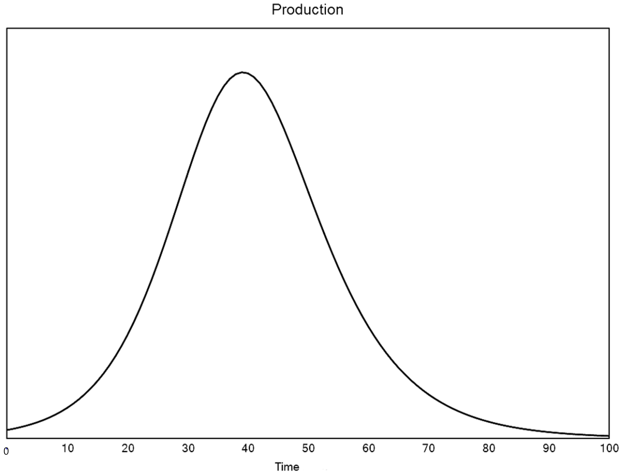
This set was termed the “single cycle Lotka-Volterra” (SCLV) model in [16]. It reproduces a “bell-shaped” curve, also known as the “Hubbert Curve.” An example of the results of the model is shown in Figure 2.

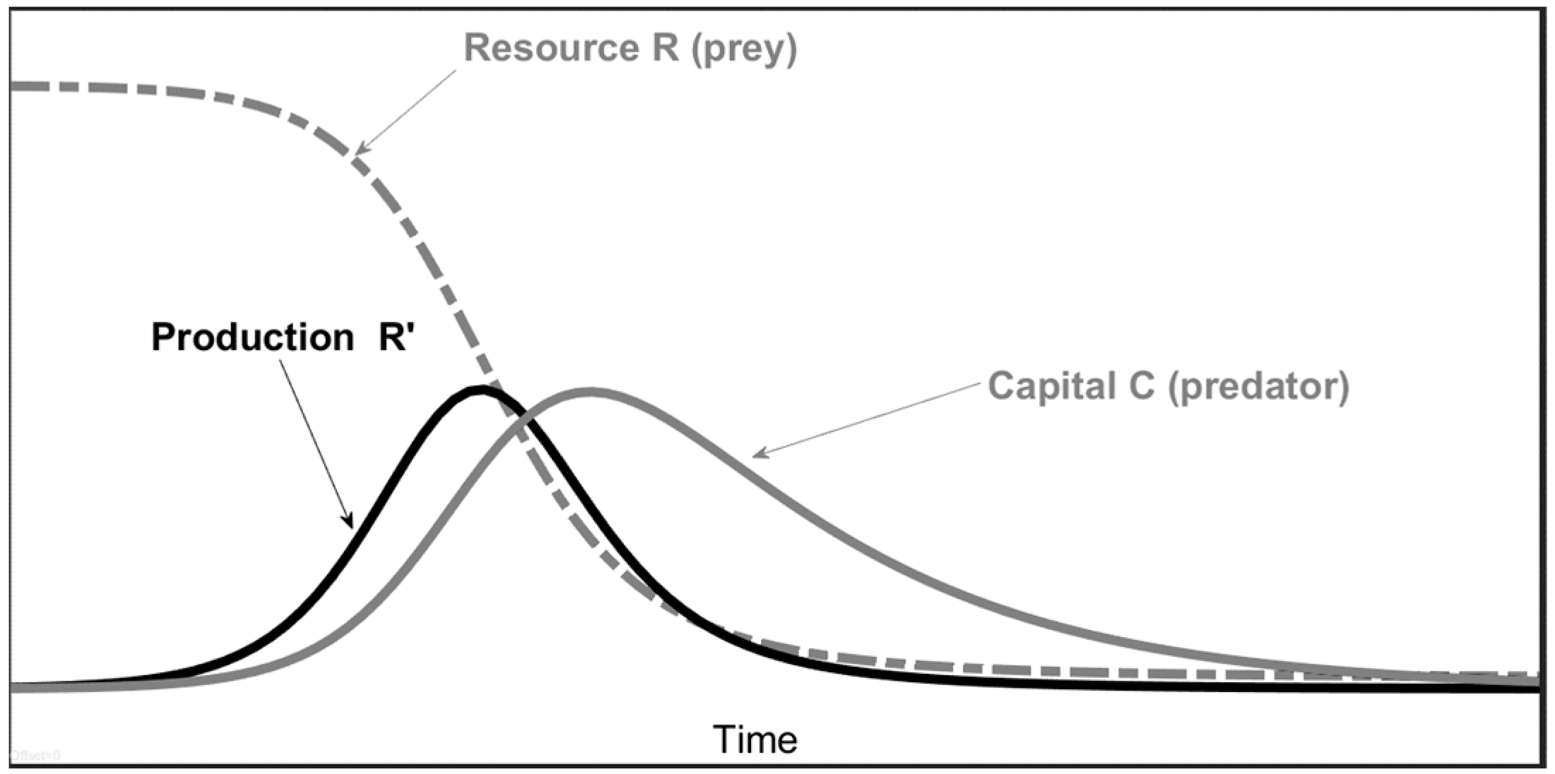
The model also generates the behaviour of the two stocks of the system, Capital and Resources. The qualitative behaviour of this system is shown in Figure 3.

In the model, the EROI can be defined as the ratio of the energy produced (that is, the flow of energy into the C stock or −ηk₂RC) divided by the energy expended (“invested”) by the capital stock (that is, the flow out of the C stock (−k₃C)). The result is as follows:

EROI = ηk₂R/k₃

(4)

The EROI value is proportional to the size of the resource stock and declines with time. By setting to zero the first derivative of Equation (2) and comparing to Equation (4), it can be proven that the capital stock peaks and starts declining when the EROI is equal to one [16]. We can write EROI_c = 1, with the “c” subscript referring to the capital peak.

Regarding the production curve, the available data are normally much more common than those for the capital curve, and so there is a special interest in determining how the EROI affects peaking. We write the EROI at the peak as EROI_p. It can be approximately determined considering that the peak occurs when about half of the URR has been extracted. Hence, R_p = ½R(0) and EROI_p = ½ηk₂R_p/k₃. Alternatively, the EROI_p can be determined by setting to zero the second derivative of Equation (3) and combining the result with Equation (4). As discussed in [16], the result is that EROI_p = k₂C_p/k₃ + 1, where, again, the “p” subscript indicates the values of the variables at the production peak. Because all the factors in this expression are larger than zero, it follows that the EROI at the production peak is larger than one. This result tells us that the production peaks earlier than the capital accumulation. This is a behaviour that agrees with the historical data.

These expressions correlate some of the parameters of the model to each other, but they do not tell us anything about the time variable. To estimate the peaking time, we need explicit time-dependent forms of the equations of the model, but such equations do not exist in a general form. Nevertheless, it is possible to simplify the model to obtain approximate expressions.

Let us start by noting that the production curve starts growing earlier than the capital curve, and so it is reasonable to assume that the capital stock (C) is small during the early stages of the cycle. In this case, the term −k₃C can be neglected. This assumption is equivalent to assuming that the growth of the stocks is exponential during the early stages of the cycle. In this case, the equations of the model are as follows:

dR/dt = −k₂RC
dC/dt = ηk₂RC

(5)

This system has an analytical solution. First, it must be that C = η (R₀ − R), with the “0” subscript indicating the value of the variables at the start of the cycle. Therefore:

dR/dt = −k₂η R (R₀ − R)

(6)

This is the well-known logistic equation, which has the integrated solution as a function of time:

R = R₀/(1 + exp(R₀k₂η(t − t₀)))

(7)

When t = t₀, the exponential is equal to 1 and we have R = ½R₀. This means that half of the resource has been extracted. The equation tp = t₀ corresponds to the peak time from the start of the exploitation cycle. This can be demonstrated by taking the second derivative of the equation for R and setting it to zero, noting that the peak corresponds to the flex of the resource curve. This interpretation implies that the production curve is symmetric, which is a reasonable approximation in many historical cases. This equality has been extensively used in early studies on oil production to estimate the data of the peak [17]. Finally, note that for R = R₀, we have t = −∞.

In the real world, t cannot be −∞, and so we can define a time (t_s (“t-start”)) that we take as the start of the cycle. We can take t₀ = 0; therefore, the “time to peak” (TtP) is −t_s. The remaining resources at t = t_s are defined as Rs.

We may now write Equation (6) as follows:

Rs = R₀/(1 + exp(R₀k₂ηts))

(8)

From this equation, we can determine the value of the t_s if we know the value of the Rs/R₀ that we call “F”, which can be calculated from the historical data. It follows that:

exp(R₀k₂ηts) = 1/F − 1

(9)

and

R₀k₂ηts = ln(1/F − 1)

(10)

TtP = t_s = ln(1/F − 1)/(R₀k₂η)

(11)

Or, also, from Equation (4):

TtP = t_s = ln(1/F − 1)/(k₃ EROI₀)

(12)

Note how the time to peak is inversely proportional to the initial EROI of the system.

We can also examine another time-dependent element generated by the model for which an analytical solution is not directly available. This is the spacing between the production peak and the peak of the capital stock. Historical data describing the latter are not often available, but when they are, the presence of the two peaks is strong evidence of the SCLV mechanism at work. We start by expressing the values of the R stock at the two peaks. Here, “p” stands for “peak production” and “c” stands for “peak capital.” To simplify, we assume η = 1:

R_p = k₃/k₂ + C_p

(13)

R_c = k₃/k₂

(14)

The difference we call ΔR_pc is equal to C_p. Because the two peaks are close to each other, we can discretize the first equation of the SCLV model and write ΔR_pc/Δt = k₂R_pC_p. Substituting, we have the following:

Δt =1/k₂R_p

(15)

There follows that the time distance between the two peaks is inversely proportional to k₂. Taking into account that EROI = ηk₂R/k₃, and that the peak occurs at approximately R_p = ½ R(0), it follows that:

Δt = µ/(EROI_p · k₃/k₂R_p)

(16)

or

Δt = 2µ/(EROI₀ · k₃)

(17)

We note that the two curves are closer to each other the larger the EROI at the start of the production cycle and the faster the depreciation takes place.

3. Results

3.1. The Mousetrap Experiment

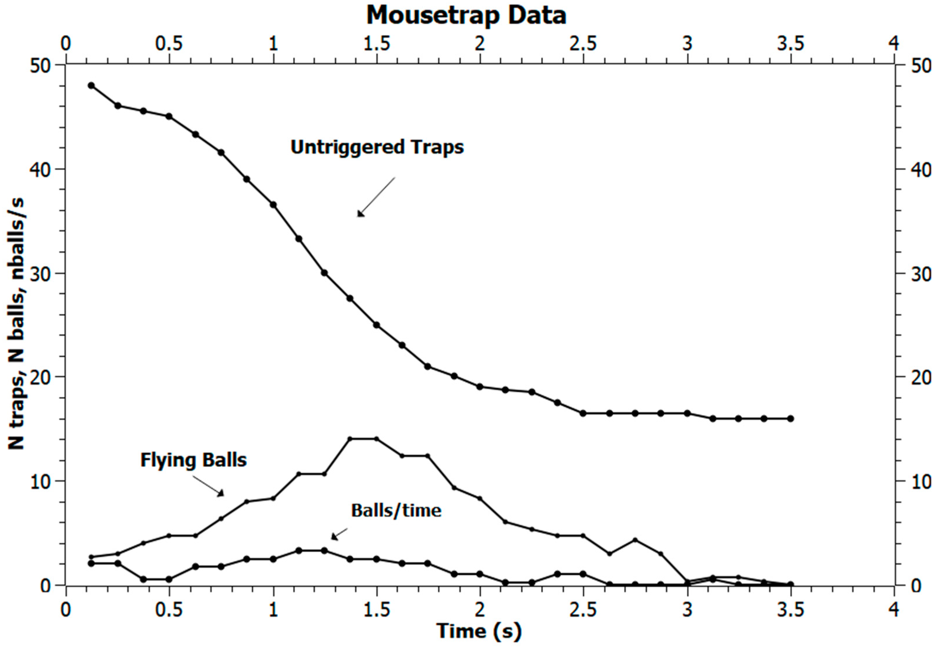
To evaluate the usefulness of the approximations developed in the previous section, we used the parameters of a real system that can be simulated using the equations reported here: the “mousetrap experiment” [11]. In this system, mousetraps loaded with wooden balls play the role of stocks of mechanical energy, while the flying balls are the result of the release of this energy that triggers more release; hence, the “capital” stock is measured by the number of flying balls at any given time. This system shows the same feedback elements as real-world systems, such as petroleum extraction, nuclear chain reactions, epidemic disease diffusion, and others. For the purposes of the present paper, it has the advantage that it is a repeatable laboratory system with parameters that are fully known.

In Figure 4, we show the measured trajectories of the main parameters of the mousetrap system in an average of three experimental tests that we ran.

By fitting the data with the SD model, we obtained the following values for the system’s parameters:

• k₂ = 0.0604 (s⁻¹*nballs⁻¹);
• η = 2;
• k₃ = 3.31 (s⁻¹);
• R₀ = 50.7 (n traps);
• C₀ = 0.6 (n balls);
• TtP = 1.2 s (time to production peak);
• TtC = 1.5 s (time to capital peak);
• 2 × 0.0604/3.31 = 0.036.

Note that the efficiency factor (µ) is larger than one. This is because the system is described in terms of “proxy” parameters (traps and balls) rather than the actual values of the energy involved.

The complete characterization of this system includes the determination of the EROI at various important points in the cycle. Note, first, that here we do not have the possibility of determining the actual elastic energy of the loaded traps, nor the kinetic energy of the flying balls. The “EROI” is a measure of the yield of the system, and, in this case, the relative yield is the ratio of the (number of balls released)/(number of balls spent). Because each flying ball releases two new balls, this ratio has to be corrected by a factor of 2. This is the η factor in the model.

To check that the above interpretation is correct, we first measure the EROI yield at the peak capital (EROI_c). We determined earlier on that this ratio must be equal to 1 if the two stocks are measured in the same units. Now, using the values obtained in the fitting, and noting that the number of untriggered traps at the peak capital is equal to ca. 26, we have EROI_c = 2 × 0.06 × 26/3.31 = 0.95, which is approximately correct.

We can now estimate the EROI₀ (the EROI at the start of the cycle). Using the same formula as before, we find that the EROI₀ = 1.82. Correctly, it is larger than one; otherwise, the chain reaction could not have started. We may also estimate the EROI_p (the EROI at the peak of the production curve). From the formula EROI_p = k₂C_p/k₃ + 1, using C_p = 11, we have EROI_p = 1.02, which is larger than the EROI_c, as it should be.

The “time to peak” (TtP) can be calculated according to the approximate formulas developed in the previous section. We said that TtP ~ ln(1/F − 1)/(R₀k₂η). F can be estimated by noting that the experiment starts with 50 traps, each loaded with 2 balls. At the start, one extra ball is dropped on the trap array—which corresponds to one-half of an additional trap. So, R_s/R₀ is 50/50.5 = 0.99. The result is TtP = 0.77 s, which is correct in terms of the order of magnitude, but smaller than the actual value of TtP = 1.15 s.

Finally, we can calculate the time difference between peak capital and peak production from the following formula: Δt = 1/k₂R_p. With R_p = 27 and k₂ = 0.0604, we have Δt = 0.6 s. Again, this value can be considered correct as an order of magnitude, but it is double the actual value, which is about 0.3 s.

In conclusion, the model provides approximate results but is correct as orders of magnitude.

3.2. Model Comparison

To evaluate the degree of approximation of the formulas proposed in the present study, we performed simulations using the full SCLV model solved by iterative approximations and compared with the approximate model.

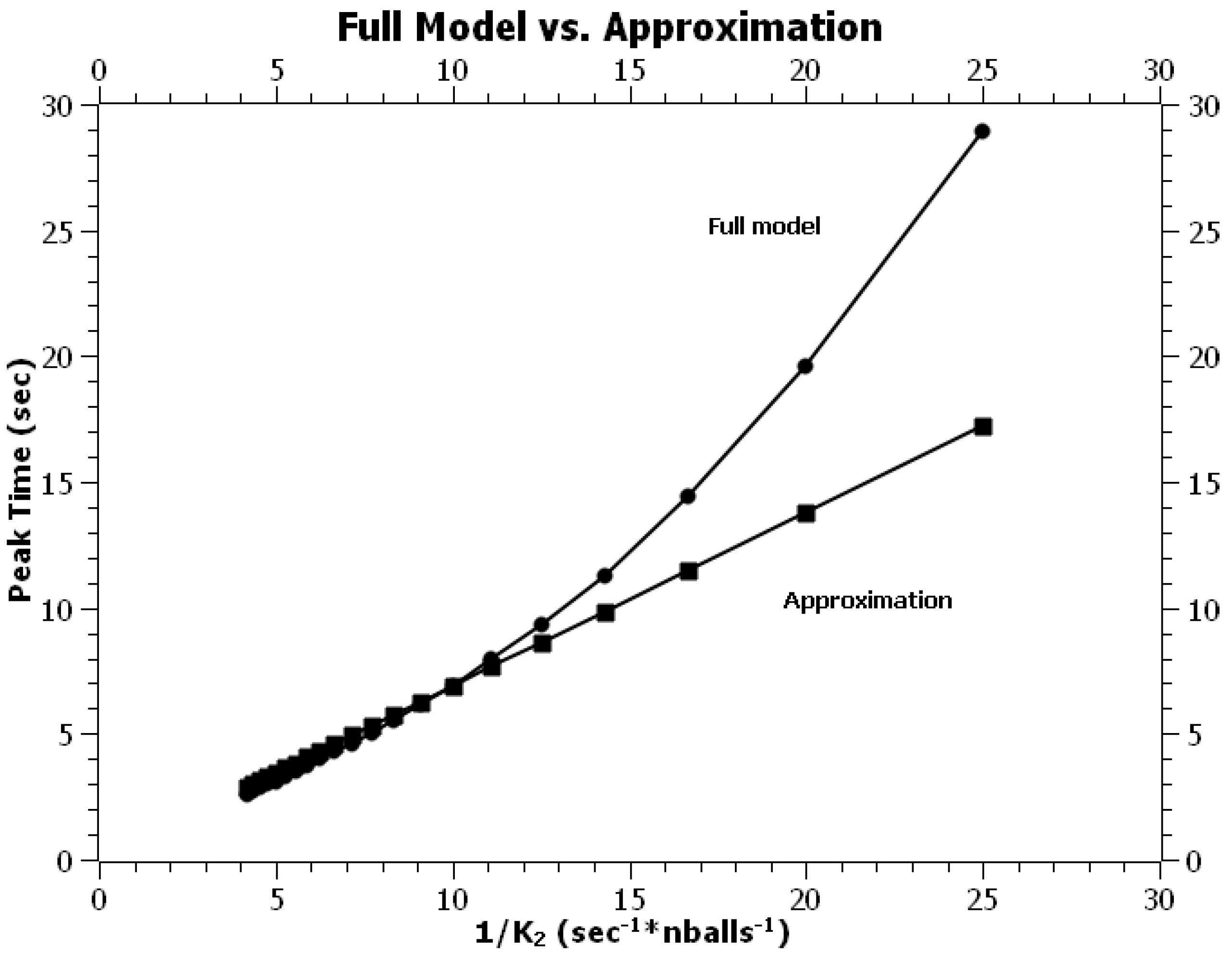
In Figure 5, we show the results for the peak time as a function of 1/k₂.

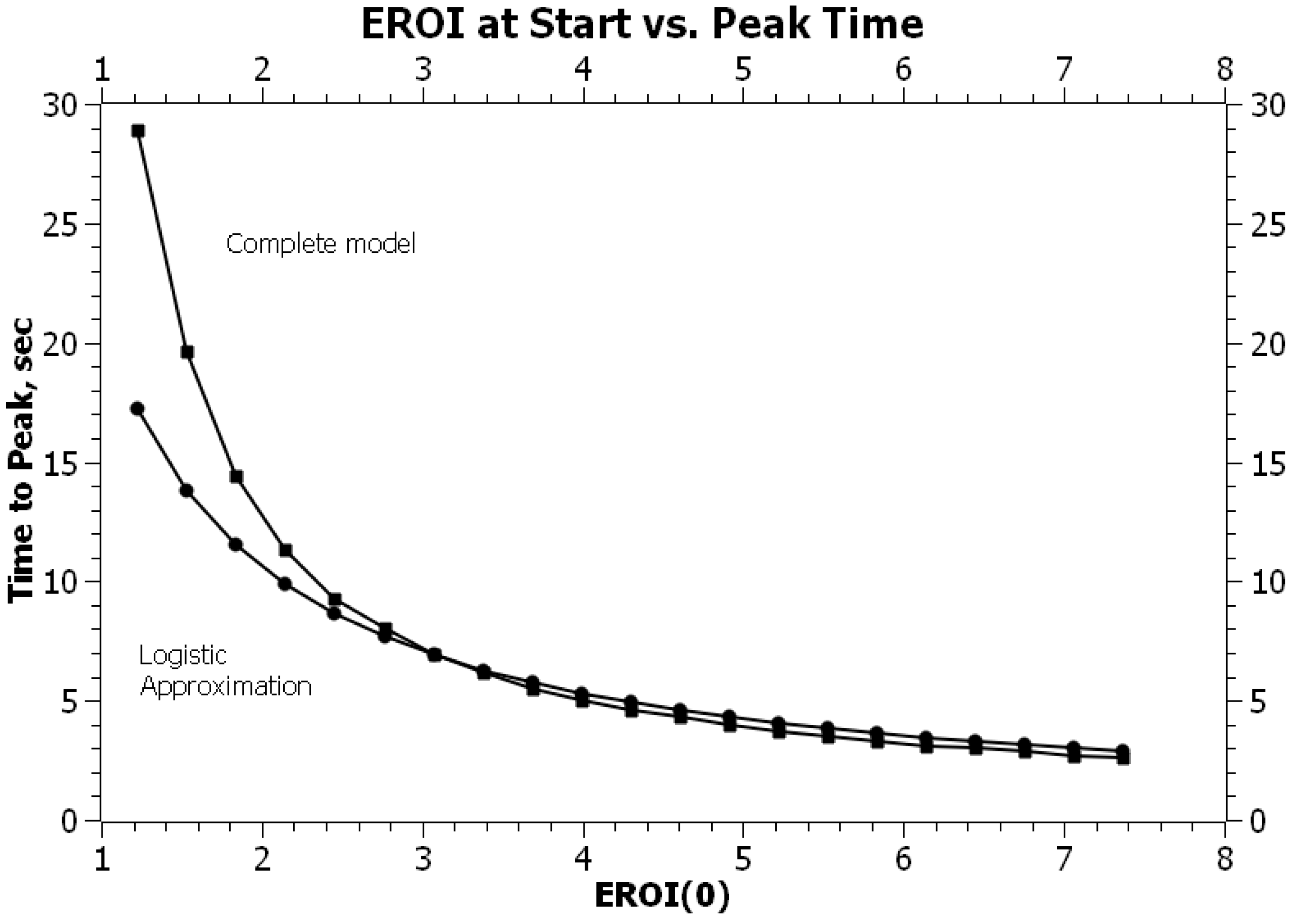
The approximation is good only for relatively large values of k, but the proportionality of the TtP (time to peak) to 1/k₂ is evident. This approximation remains valid if we express the time to peak as a function of the value of the EROI at the start of the cycle (EROI₀), as shown in Figure 6.

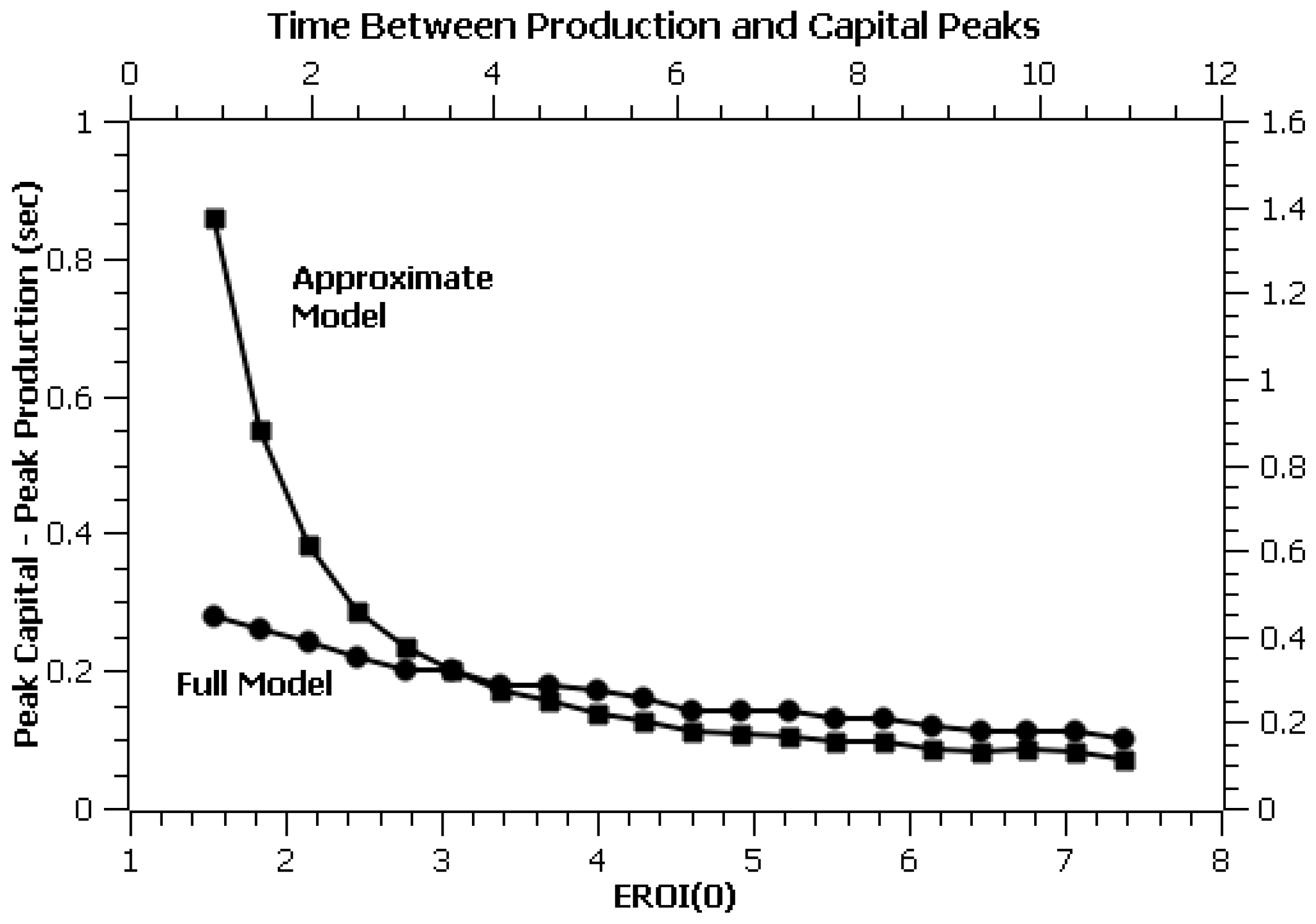
Finally, we tested the dependency of the time distance between the production peak and capital peak. The results are shown in Figure 7, and they confirm that the peaks become closer together for larger values of the initial EROI of the system. Note, though, that the discrepancy of the full model with the approximate model is large for low EROIs, which is consistent with the results obtained with the mousetrap experiment, where the EROI is relatively small.

4. Conclusions

Models are a popular way to understand and manage complex realities. They can be used in basically two ways: one way is to interpret data, and the other is to predict the future. Both are subjected to uncertainties, given the many uncertainties in data and the effects of human factors, such as political decisions, financial effects, and technological factors. However, predicting the future is a difficult task, and there are many cases of failed predictions. Regarding the subject of this study, predicting the future of mineral production has turned out to be difficult. A large number of studies have attempted to provide an answer, and the range of dates proposed is wide, spanning at least a couple of decades. Models failed to predict the rapid growth of nonconventional oil production in the United States, which changed the whole world’s trends and postponed the peak by at least a decade.

What models can do, however, is interpret the past, and the past is always a guide to the future. One shortcoming of many studies on resource production is the lack of a model that interprets the reasons why the exploitation cycle follows a specific path in relation to the physical parameters of the system, such as its energy yield in the case of the extraction of fossil fuels. In this light, the use of the SCLV model to describe the peaking of the production of a nonrenewable resource highlights a fundamental element of the overexploitation phenomenon. We were able to model some parameters that, to the best of our knowledge, were never reported in previous studies on these kinds of biophysical models. The model we developed is necessarily approximate, but it can be used to determine some “rules of thumb” for understanding the peaking phenomenon in the exploitation of natural resources.

The present paper is limited to the examination of a “toy” model as a test bed for the formulas and concepts that we developed. This approach was chosen as a first demonstration that the model can be useful to examine a real-world system. The usability of the model for predictive purposes is still to be tested and examined. Generally speaking, no model can be more accurate than the data that are input, and so extrapolating trends from a limited database is always risky. Our model is no exception to this rule, and it is affected by uncertainties in the historical data, and by all the factors that make predictions difficult when we deal with systems that are influenced by political decisions. For these reasons, we do not claim that our method is better than the simpler ones used so far in peak-oil studies (e.g., “Hubbert Linearization”). Instead, we believe that the main innovative element of the present study, and its fundamental purpose, is the demonstration of the influence of the input parameters on the production cycle length and intensity. In particular, we demonstrate that the duration of the production cycle is inversely proportional to the initial EROI (energy return for energy invested) of the exploitation process. In other words, for the same amount of available resources, systems providing larger initial energy or economic returns are more rapidly overexploited and depleted.

Further research is in progress to examine the historical exploitation cycles of natural resources, including metal ores and rare-earth elements.