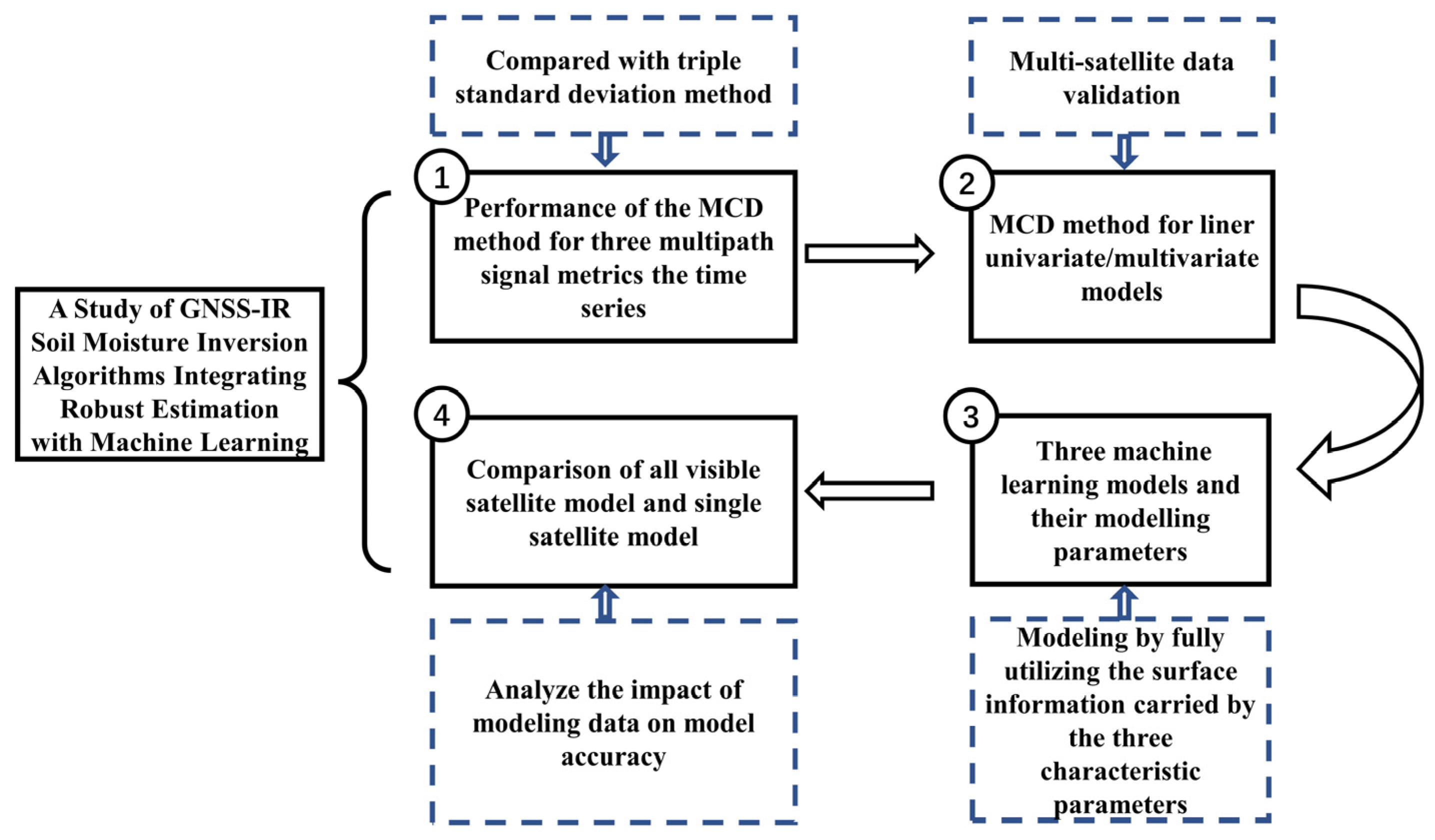
A Study of GNSS-IR Soil Moisture Inversion Algorithms Integrating Robust Estimation with Machine Learning

Abstract

Soil moisture monitoring is widely used in agriculture, water resource management, and disaster prevention, which is of great significance for sustainability. The global navigation satellite system interferometric reflectometry (GNSS-IR) technology provides a supplementary method for soil moisture monitoring. However, due to the quality of the signal-to-noise ratio (SNR) measurements and the complex surface environment, inevitable outliers in multipath interference signal metrics (amplitude, frequency, and phase) were used as modeling variables to inverse GNSS-IR soil moisture. Besides, it is hard to use the univariate model to comprehensively analyze the relationship between the various factors, due to the poor fitting effect and weak generalization ability of the model. In this paper, the minimum covariance determinant (MCD) robust estimation and machine learning algorithms are adopted. The MCD robust estimation can eliminate outliers of the multipath signal metrics and machine learning algorithms, including the back propagation neural network (BPNN), Gaussian process regression (GPR), and random forest (RF), and can comprehensively establish nonlinear GNSS-IR soil moisture inversion models using multipath interference signal metrics. Moreover, the study of the modeling parameter selection for the three machine learning algorithms and the inversion results for single satellite and all satellites are also carried out to make the algorithms more generalizable. The results show that the correlation coefficients (R) and the root mean square error (RMSE) of the machine learning models for all satellite tracks are increased by 4.3~86.6% and reduced by 2.8~30%, respectively, compared with the MCD multiple regression model. The RF model with 80 decision trees and 1 node shows the clearest improvement. The total model using all satellite data has more generalization ability than the single satellite model but causes some loss of accuracy.

1. Introduction

Soil moisture is a crucial variable of the climate system, which affects plant transpiration and photosynthesis, and has implications for the sustainability of water resources and biogeochemical cycles. Therefore, it is necessary to have timely and accurate soil moisture information [1,2,3]. Traditional soil moisture measurement methods, such as the in situ soil hygrometer, are accurate but consume much labor and material resources and have long measurement cycles [4]. Although remote sensing technologies can overcome the disadvantage of small coverage area of traditional soil moisture monitoring methods, the temporal resolution is not ideal [5,6]. Therefore, GNSS-IR technology based on the interference of GNSS direct and reflected (multipath) signals recorded as the signal-to-noise ratio, with its high temporal and spatial resolution, has gradually become a promising technology for soil moisture monitoring and has attracted widespread attention [7,8,9].

GNSS-IR technology was developed from GNSS Reflectometry (GNSS-R), a passive noncooperative bistatic radar that enables the inversion of physical surface parameters by processing the reflected signal [8,10]. GNSS-R was first proposed by Hall and Cordey for ocean remote sensing research in which the GNSS signal reflected by the ocean is equivalent to a scatterometer [11]. The signal-to-noise ratio (SNR) is the ratio of the signal power to the noise power. Due to the multipath effect, the SNR contains the variation of the interference signal formed by the direct signal and the multipath signal [12,13]. Therefore, GNSS-IR technology, a new mode of GNSS-R, was proposed, which is different from the traditional dual antenna mode, using a right-hand circularly polarized (RHCP) antenna to receive the SNR data to detect physical surface parameters [14]. An algorithm of soil moisture inversion was investigated using the SNR observations recorded using a geodetic-grade GPS receiver and meteorological data [15,16,17]. The results showed that the frequency of the SNR of a multipath signal is related to the effective antenna height, and the amplitude and phase of the SNR are related to the soil moisture, which can be used to monitor soil moisture in a large area through a network of GPS stations. Furthermore, the strong correlation between the multipath signal SNR phase, amplitude, and effective height calculated from the frequency and the soil moisture from the plate boundary observatory (PBO) (https://gnss-h2o.jpl.nasa.gov/index.php, accessed on 1 December 2020) was verified [18]. Roussel et al. analyzed the effect of GPS and GLONASS satellite altitude angles on the soil moisture inversion of different metrics for multipath signals by inverting the time series of high elevation angles and combining them with low elevation angle time series, which significantly improved the correlation between the soil moisture and the phase [19]. Vey et al. constructed an empirical model for soil moisture inversion with a long SNR time series and found that the inversion results of the GPS L2C signals are better than those of the GPS L1C and L2W signals [20]. Vegetation is usually present on the ground and can affect GNSS signals. The L-band signal used in GNSS-IR also has a certain penetration ability for vegetation. Its signal intensity and propagation time will change due to the influence of the vegetation during different growing periods, whereby the amplitude of the multipath signal is related to vegetation water content or height [17]. Good agreement was shown between the GPS multipath signal metrics and field observations of vegetation height and vegetation water content [21]. The amplitude of the multipath signal shows a nearly linear relationship to the water content in grasses and wheat crops [22]. Affected jointly by soil moisture and vegetation water content, GNSS multipath signals carry both soil moisture and vegetation information. It is not rigorous to inverse soil moisture or vegetation water content alone. Other SNR metrics except phase can be used to characterize vegetation effects. Amplitude decreases as vegetation grows [21]. Unfortunately, the current research on GNSS-IR soil moisture inversion is mostly focused on linear modeling to quantify the functional relationship between the soil moisture and a certain characteristic metric of multipath signals, ignoring the reflection surface information carried by the other two metrics. Besides, due to the quality of the SNR and surface environmental characteristics, and error propagation during data processing, outliers are inevitably present in SNR metrics [10,21,23]. Several methods have been proposed to attenuate the effects of vegetation [22,24], but these methods require auxiliary data, such as prior soil moisture information and surface conditions, to ensure their effectiveness. In addition, the surface environment factors such as surface roughness, vegetation, and temperature can also influence the soil moisture estimation [25]. Moreover, the coupling of surface environmental factors forms a complex nonlinear problem, which is difficult to consider comprehensively.

Machine learning algorithms can train input–output data to establish their mapping relationships, which is suitable for building models with nonlinear and implicit relationships. It is worth mentioning that outliers in input data will affect the machine learning modeling effect. In recent years, machine learning algorithms have shown great application prospects for remote sensing [26]. Random forest and support vector machine algorithms were used to retrieve soil moisture with GNSS-R data [27]. The soil moisture products for tropical regions based on machine learning were provided using U.S. cyclone global navigation satellite system (CYGNSS) satellite data [28,29]. The coastal wind speed in China was analyzed based on artificial neural networks and CYGNSS data [7]. A multi-satellite fusion sliding estimation method of soil moisture was established with the least squares-support vector algorithm [30]. However, most of the studies focused on GNSS-R technology, and studies on the research and application of machine learning for GNSS-IR are even more scarce.

GNSS-IR soil moisture inversion methods integrating robust MCD estimation with machine learning algorithms are proposed to solve the following limitations in existing GNSS-IR soil moisture inversion modeling studies: (1) outliers in the observations; (2) the difficulty in quantitatively studying the influence of a complex surface environment; and (3) the characteristics of the multipath signal not being fully taken into consideration. First, MCD robust estimation is used to detect outliers of the time series of the multipath signal metrics. Machine learning algorithms are introduced to utilize all characteristic metrics to establish a nonlinear model between all the GNSS multipath signal metrics and the soil moisture. The parameter selection of machine learning algorithms in the modeling process is also analyzed in detail. Finally, the nonlinear robust machine learning model is verified by using PBO observation data. The inversion accuracies of nonlinear robust machine learning models and linear robust multiple regression models are compared, and the inversion results of different satellite data are analyzed.

The paper proceeds as follows: Section 2 describes the study area and introduces the data resources; Section 3 introduces the theoretical background and linear method of GNSS-IR soil moisture inversion; Section 4 presents the inversion models integrating the robust estimation method with machine learning algorithms and analyses the modeling process; Section 5 provides results, data analysis, and a performance comparison; Section 6 presents a discussion.

2. Study Area and Data Resource

The PBO has more than 1000 continuously operating high-precision GPS stations for geodetic measurements around the world, most of which are located in the western United States and can provide high-quality L2-band SNR observations, as well as higher resolution meteorological observations such as relative humidity, precipitation, temperature, and barometric pressure [31].

The observation data of the PBO network’s P043 station from 18 January 2016 to 30 September 2016 were selected for the experiments (The rising satellite tracks are used, since the interferogram pattern can differ for rising and setting tracks of the same satellite) [32]. We use the first 75% of data as the training set and the last 25% of data as the test set to model the GNSS-IR soil moisture inversion model. The P043 station is located at 43.881146 W, 255.814298 N, with an altitude of 1490.9 m. The TRIMBLE NETRS dual-band network receiver was used, and its location and surrounding environment are shown in Figure 1a,b. The surface vegetation cover type around the P043 station is grassland. The terrain around the station is relatively flat. At the same time, the annual snowfall at this station is low, which reduces the impact of snow on soil moisture inversion and meets the experimental requirements. The sensing area of satellite tracks for P043 is about 100 m² [33]. The soil moisture from the PBO network was used as a reference value for the subsequent inversion studies [34,35,36].

3. Methodology

3.1. Theoretical Background of GNSS-IR Soil Moisture Linear Inversion

The surface reflection properties of the surface determine the interference phenomenon. Therefore, the physical properties can be inversely determined using the interference signal. The GNSS signal received by the ground-based receiver with single-antenna is the interference signal of the direct signal and the reflected signal, which can be expressed using SNR as [15,16]

$$SN{R}^2=A_c{}^2=A_d{}^2+A_m{}^2+2A_d{A}_m\cos \psi$$

(1)

where $A_d$ denotes the amplitude of the direct signal, $A_m$ represents the amplitude of the multipath signal, $A_c$ is the amplitude of the composition signal, ${\phi }_d$ denotes the phase of the direct signal, ${\phi }_c$ denotes the phase of the vector composition signal, and $\psi ={\psi }_c-{\psi }_d$ denotes the phase difference between the direct and reflected signals.

The power of the direct signal is much larger than that of the reflected signal. The observations of the interference signal are obtained by removing the direct signal using a low-order polynomial fitting. The reflected $SN{R}_m$ observations and $\sin \theta$ can be fitted by a cosine function with a fixed frequency:

$$SN{R}_m=A_m\cos \left(\frac{4\pi h}{\lambda }\sin \theta +\phi \right)$$

(2)

where $\theta$ denotes the satellite elevation angle, $h$ denotes the effective antenna height, $\lambda$ denotes the satellite signal wavelength, and $\phi$ denotes the phase offset. The effective antenna height is calculated by Lomb–Scargle Periodogram, and the oscillation frequency $f$ is calculated by

$$f=2h/\lambda$$

(3)

The oscillation frequency $f$, phase $\phi$ and amplitude $A_m$ of the multipath signal can be obtained by using the above methods. Larson et al. [15,16] demonstrated that all three metrics have a certain correlation with soil moisture. The most used method to construct a GNSS-IR soil moisture inversion model is dividing the metrics of the multipath signal into two parts: a training set and a test set. A linear regression model of the metrics and the soil moisture is constructed by the least squares method with the training set. Then, the test set is used to obtain the soil moisture prediction value. The validity and accuracy of the model are evaluated by correlation coefficient (R), root mean square error (RMSE), and mean absolute error (MAE).

3.2. Soil Moisture Inversion Algorithm Fusing Robust Estimation and Machine Learning

3.2.1. MCD Robust Estimation

Due to the quality of the SNR and surface environmental characteristics, and error propagation during data processing, outliers are inevitably present in SNR metrics [10,21,23].

The MCD estimation method is a location and distribution estimation algorithm. It constructs a robust covariance matrix estimator by iteration and the Mahalanobis distance and then iteratively solves the Mahalanobis distance and uses the chi-square test to detect the presence of outliers in the observed data and assign them different weights [37].

For a dataset $X_n=\left\{X_1,X_2,\cdot \cdot \cdot ,X_n\right\}$ with $n$ samples, each sample has $p$ elements. $h$ samples are randomly selected from the dataset; usually, the default value of $h$ is $0.75n$. The mean value $u_1$ and the covariance matrix $S_1$ of the $h$ samples are the initial mean and the initial covariance matrix.

$$u_1=\frac{1}{h}{\displaystyle \sum _{i=1}^h{X}_i}$$

(4)

$$S_1=\frac{1}{h}{\displaystyle \sum _{i=1}^h\left(X_i-u_1\right){\left(X_i-u_1\right)}^T}$$

(5)

The Mahalanobis distances between the dataset and the center of the $h$ samples are calculated by the mean and covariance of the $h$ samples.

$$MD\left(i\right)=\sqrt{{\left(X_i-u_1\right)}^T{S}_1{}^{-1}\left(X_i-u_1\right)}$$

(6)

The $n$ calculated Mahalanobis distances are sorted. Then, the $h$ samples with the smallest distance are selected. The mean estimate $u_2$ and covariance matrix estimate $S_2$ of the $h$ samples are calculated. The above process is repeated until $\det \left(S_i\right)=\det \left(S_{i-1}\right)$ or $\det \left(S_i\right)=0$. The relationship between the determinants of the covariance matrices during the iteration is

$$\det \left(S_1\right)\ge \det \left(S_2\right)\ge \cdots \ge \det \left(S_{i-1}\right)\ge \det \left(S_i\right)$$

(7)

The mean and covariance matrices calculated in the last iteration are the robust mean estimate ${\widehat{u}}_{\mathrm{MCD}}$ and the robust covariance estimate ${\widehat{S}}_{\mathrm{MCD}}$, and the robust Mahalanobis distance $RD(i)$ of the dataset can be obtained.

$$RD(i)=\sqrt{{\left(X_i-{\widehat{u}}_{\mathrm{MCD}}\right)}^T{\widehat{S}}_{\mathrm{MCD}}^{-1}\left(X_i-{\widehat{u}}_{\mathrm{MCD}}\right)}$$

(8)

$RD(i)$ obeys the chi-square distribution with degree of freedom $p$. When $RD\left(i\right)>\sqrt{{\chi }^2{}_{p,\alpha }}$, the corresponding sample can be considered an outlier. The opposite is the normal value. For example, when confidence $\alpha =0.975$ and degrees of freedom $p=1$,$\sqrt{{\chi }^2{}_{1,0.975}}=2.2414$. Therefore, when the robust Mahalanobis distance $RD\left(i\right)>2.2414$, the corresponding sample is an outlier.

3.2.2. Machine Learning Algorithms

The majority of previous soil moisture inversion studies were based on assumptions such as flat reflection surfaces and did not fully consider the complex environment around the reflection surface. It is difficult to quantitatively analyze the effects of multiple environmental factors on multipath signals, and a linear model cannot accurately express the complex relationship between metrics and soil moisture. Machine learning algorithms can train input-output data to establish their nonlinear mapping relationships, which is suitable for building models with nonlinear, implicit relationships. Therefore, the GNSS-IR soil moisture inversion model was established based on the robust estimation MCD method combined with machine learning algorithms to suppress the effects caused by environmental factors and obtain continuous and accurate soil moisture measurements.

• Backward Propagation Neural Network

In the BPNN algorithm, the signal propagates forward, and the error propagates backward. The model adjusts the weights of the negative gradient direction of the RMSE for a single sample using the gradient descent approach, which is suitable for solving complex nonlinear problems and has good adaptive capability but is prone to problems such as locally optimal solutions, slow convergence, and dependence on sample data [38]. The basic principles and algorithmic process of the standard BPNN algorithm are briefly described using a three-layer neural network structure.

The back propagation process of the BPNN is essentially an iterative learning process. Each iteration updates the threshold and weight of the network until the required mean square error is satisfied, at which time the iterative process is stopped. More details of the BPNN can be found in the literature [11,35].

Larson et al. [16] pointed out that every multipath signal characteristic metric has a certain correlation with soil moisture, and the inversion accuracy of the phase model is higher than that of the frequency and amplitude models. The input layer sample parameter $x_i=[f,A_m,\phi ]$ is created to fully use the multipath signal, where $f,A_m,\phi$ are the frequency, amplitude and phase of the multipath signal, respectively. The output layer sample parameter $y_i$ is the reference soil moisture value. Before training the training set, the type of activation function and the number of neurons in the hidden layer must be chosen to build the best BPNN model. The empirical formula for the number of neurons in the hidden layer is [39]

$$m=\sqrt{n+q}+a$$

(9)

where $m$ represents the number of neurons of the hidden layer, $n$ represents the number of the input layer, $q$ represents the number of the output layer, and $a$ is a positive integer between [1,10]. In our tests, we found that the ‘Sigmoid’ function is most suitable for the GNSS-IR soil moisture inversion algorithm. ‘Tansig’, ‘Logsig’, and ‘Purelin’ are the commonly used ‘Sigmoid’ activation functions [39].

2.

Gaussian Process Regression

From the training samples, the GPR algorithm can identify the mapping relationship between the input and output values, establish their mapping function, and then predict the optimal output value corresponding to the input value in the test set. A GPR algorithm easily achieves adaptive acquisition of hyper parameters, and its output values have probabilistic significance, which works well for addressing nonlinear, high dimensional, difficult regression problems with small samples. Although it is capable of broad generalization, it is prone to local optimal solutions [40,41]. The main principles are as follows.

The covariance function is the main determinant of a Gaussian process (GP), which is a collection of random variables that follow a joint Gaussian distribution. The covariance function can be used to obtain the covariance matrix, so the selection of the covariance function is crucial and plays a role in determining the prediction accuracy of the GPR. Common kernel functions include the squared exponential kernel, exponential kernel, and Matérn (Matérn 32, Matérn 52) kernels. More details on the GPR algorithm can be found in the literature [41].

3.

Random Forest

The random forest is a tree classifier that trains and predicts samples through multiple decision trees. A random forest can handle complex nonlinear problems, has fast computational speed and strong generalization ability, and is less prone to local optima and overfitting [42].

The core of establishing the decision tree is how to perform the best node splitting. A random forest regression uses the CART algorithm, which determines the best node splitting based on the principle of minimum root mean square error, to complete the establishment of the decision tree. The difference between a random forest and a single decision tree is that in the selection of the number of features, several features are selected randomly instead of all of them, and then, the optimal one is selected from them, which improves the diversity of a random forest, effectively avoids the overfitting phenomenon, and improves the prediction accuracy. After all the decision trees have been constructed, they are integrated into a random forest regression model. The predicted value of the test set is the mean value of all the decision tree outcomes.

4. Experiments and Results

Figure 2 illustrates the framework and experimental design of the proposed GNSS-IR soil moisture inversion algorithms integrating robust estimation with machine learning. Firstly, the performance of the minimum covariance determinant (MCD) method and conventional triple standard deviation method for the time series of three multipath signal metrics is analyzed. Secondly, the effectiveness of the MCD method for modeling liner univariate/multivariate models is validated with all visible satellites data, and the necessity of modeling using multiple feature parameters is demonstrated. Then, modeling by fully utilizing the surface information carried by the three characteristic parameters with three machine learning algorithms and, at the same time, the study of the modeling parameter selections for machine learning algorithms are carried out. Lastly, the impact of modeling data on model accuracy is analyzed by comparing the accuracy of all visible satellite models and single satellite models.

4.1. MCD Robust Estimation for Soil Moisture Inversion

The MCD method and conventional triple standard deviation method ($3\sigma$) are used to denoise the time series of three multipath signal metrics for all visible satellites.

The detection results of the amplitude, frequency, and phase time series for all satellites are shown in Figure 3. Taking the PRN 17 as an example, the ability of two methods to detect outliers is shown in Figure 4. Linear modeling is carried out with the denoised time series of metrics, respectively. RMSE is used to compare the effectiveness of the two robust estimation methods and is shown in Figure 5. Figure 3 shows that the MCD method exhibits stronger detection of multipath signal metric outliers than the $3\sigma$ method. According to the experimental results, the MCD method can detect not only the outliers already identified using the conventional method but also the outliers missed by the conventional method. Figure 4 shows that the judgment criterion of the MCD method and $3\sigma$ method, the red line in the figures, can distinguish abnormal values and normal values more clearly. Figure 5 illustrates that the accuracy of the models established with the multipath signal metrics time series, which denoised by using the MCD method, is generally improved. This is further evidence that the triple standard deviation method may be inadequate for detecting certain noise, which may significantly affect the model accuracy. In general, in the GNSS-IR soil moisture inversion study, the triple standard deviation method for outlier detection of the metrics may be susceptible to the effect of outlier masking, which shifts the calculated standard deviation and leads to inaccurate detection results of outliers and missing judgment. The detection of outliers via the MCD method, whose robust Mahalanobis distance is calculated from the mean and covariance matrix of the samples solved iteratively, can greatly reduce the influence of the outliers.

4.2. Robust Multiple Regression Model for Soil Moisture Inversion

In this section, consistent with above, the inversion results of the PRN 15, 17, 31 satellites are selected as examples. Since the metrics $f$, $\phi$, and $A_m$ of the multipath signal are all correlated with soil moisture, to fully and effectively utilize the information of multiple characteristics, a robust multiple regression model based on the MCD robust estimation and linear regression method was developed in the manuscript and used to compare the linear regression models of the frequency, amplitude, and phase. Their inversion results are statistically analyzed, as shown in

Table 1. Linear soil moisture inversion models based on the MCD method.

Satellite Tracks	Variable	Model Equation	Correlation Coefficient	Root Mean Square Error (cm3/cm3)
PRN 15	Frequency	$y=-0.0712x+1.2971$	0.2844	0.0649
	Amplitude	$y=0.0989x-0.1553$	0.4949	0.0580
	Phase	$y=0.0135x+0.1161$	0.5019	0.0591
	Multiple	$y=-0.0063x_1+0.0271x_2+0.0110x_3+0.1424$	0.6366	0.0520
PRN 17	Frequency	$y=-0.1052x+1.8371$	0.4512	0.0615
	Amplitude	$y=0.0290x+0.2221$	0.3124	0.0630
	Phase	$y=-0.3642x+0.2653$	0.4436	0.0634
	Multiple	$y=-0.0441x_1-0.0312x_2-0.3144x_3+1.0356$	0.7890	0.0438
PRN 31	Frequency	$y=-0.0875x+1.5402$	0.5052	0.0589
	Amplitude	$y=0.0765x-0.0109$	0.5389	0.0590
	Phase	$y=-0.2160x+0.3420$	0.3265	0.0674
	Multiple	$y=-0.0153x_1+0.0630x_2-0.1608x_3+0.4049$	0.6168	0.0548

. The RMSE values of the four models for all visible satellites are also displayed in Figure 6 to demonstrate the validity of the robust multiple regression model.

Table 1 and Figure 6 show that the inversion accuracy of the univariate soil moisture models is poor, and the optimal model is uncertain. The inversion accuracy of the multiple regression model based on the MCD method is significantly better than those of the univariate regression models. The reason for the poor inversion accuracy of the univariate model may be the coupling effect of surface vegetation and surface roughness. By contrast, the multiple regression model based on the MCD can somewhat weaken the influence of multiple surface information on soil moisture inversion, fully utilizing the information of the multipath signal for GNSS-IR soil moisture inversion and improving the inversion accuracy significantly.

4.3. Machine Learning Models for Soil Moisture Inversion

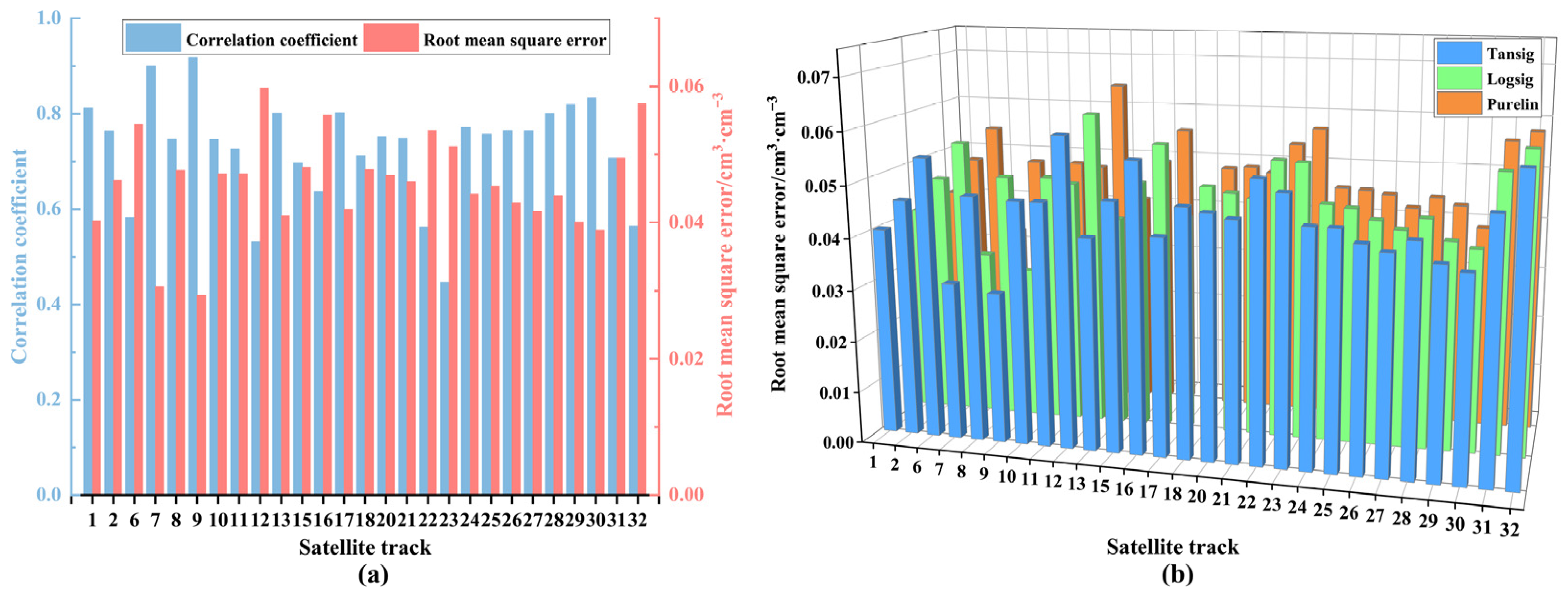
4.3.1. Hyper Parameters Selection of the Backward Propagation Neural Network Model

The observations of the PRN 31 from 18 January 2016 to 30 September 2016 were randomly selected as example data.

Table 2. Inversion results of the different neuron numbers for the PRN 31 satellite using the BPNN model.

Hidden Layer	R	RMSE (cm3/cm3)	Hidden Layer	R	RMSE (cm3/cm3)
3	0.6847	0.0517	9	0.6889	0.0513
4	0.6807	0.0513	10	0.6900	0.0509
5	0.6896	0.0514	11	0.6730	0.0515
6	0.7065	0.0495	12	0.6760	0.0516
7	0.6916	0.0515	13	0.6581	0.0525
8	0.6633	0.0523	14	0.6633	0.0524

displays the differences in R and the RMSE when various numbers of neurons are selected.

Table 3. Inversion results of the different activation functions for the PRN 31 satellite using the BPNN model.

Activation Function	R	RMSE (cm3/cm3)
Tansig	0.7065	0.0495
Logsig	0.6460	0.0536
Purelin	0.6027	0.0564

displays the inversion results of the PRN 31 satellite with different activation functions when the learning efficiency, the number of iterations, the expectation error, and the number of neurons for the hidden layer are all equal.

Table 2 and Table 3 show that the correlation coefficient R of the BPNN model is at its maximum value of 0.7065 and the RMSE is at its lowest value of 0.0495 when the number of hidden layers is 6. Therefore, six hidden layer neurons are the ideal quantity for the PRN 31 satellite. The highest BPNN model accuracy is achieved when the ‘Tansig’ function is used as the activation function. Therefore, the ‘Tansig’ function is utilized as the activation function to construct the BPNN inversion model for the PRN 31 satellite at the P043 station. Similarly, the activation functions for other satellites and their numbers of hidden layer neurons can be determined. The ‘Tansig’ function is shown to be the best for all satellite data, although the number of hidden layers is not constant. For instance, 4 and 8 hidden layers are the ideal amount for the PRN 15 and PRN 17 satellites, respectively. The inversion results of all visible satellites with different BPNN models are shown in Figure 7. As shown in Figure 7a, the BPNN algorithms are able to construct the GNSS-IR soil moisture inversion models effectively (R > 0.5) for almost all visible satellites data. Although there is a difference in the optimal number of hidden layers for different satellites, Table 2 demonstrates that the number of hidden layers has little effect on the inversion accuracy. In view of this, to extend the generalizability of the algorithm, we set the number of hidden layers to 6 and compare the performance of the three activation functions when modeling different satellite data. The results are displayed in Figure 7b. As seen in Figure 7b, when the number of hidden layers is set to 6, all three activation functions can effectively establish soil moisture inversion models for different satellite data, and the ‘Tansig’ function has the highest inversion accuracy. Therefore, the six hidden layers and the ‘Tansig’ activation function can be used as the default parameters for BPNN to construct GNSS-IR soil moisture inversion models.

4.3.2. Hyper Parameters Selection of the Gaussian Process Regression Model

The selection of the kernel function for constructing the GPR soil moisture inversion model affects the prediction accuracy. Five functions, the squared exponential kernel function, exponential kernel function, Matérn kernel functions, rational quadratic kernel function, and ARD exponential kernel function, were selected. The observations of the PRN 31 were randomly selected as example data.

Table 4. Inversion results of the different kernel functions for the PRN 31 satellite using the GPR model.

Kernel Function	R	RMSE (cm3/cm3)
Squared exponential kernel	0.7225	0.0492
Exponential kernel	0.7543	0.0474
Matérn 32 kernel	0.7524	0.0478
Matérn 52 kernel	0.7472	0.0477
Rational quadratic kernel	0.7559	0.0475
Ard exponential kernel	0.7874	0.0455

shows the inversion results.

From Table 4, the inversion accuracy of the GPR model with the ARD exponential kernel function for the PRN 31 satellite is the highest, with an improvement of 8.92% compared to the squared exponential kernel function. The rational quadratic kernel and exponential kernel also achieve relatively better results.

To extend the generalizability of the algorithm, the inversion results of all visible satellites with different GPR models are shown in Figure 8. The inversion results of all other visible satellites with the ARD exponential kernel function are shown in Figure 8a. We compare the performance of the three kernel functions when modeling different satellite data. The results are shown in Figure 8b. From Figure 8, the GPR algorithms with the three kernel functions are able to construct the GNSS-IR soil moisture inversion models effectively (R > 0.5) for all visible satellites data. The inversion accuracy of the GPR model with the ARD exponential kernel function for all satellites is the highest. Therefore, the ARD exponential kernel function can be used as the default parameter for GPR to construct GNSS-IR soil moisture inversion models.

4.3.3. Hyper Parameters Selection of the Gaussian Process Regression Model

The number of decision trees and the number of node variables of the decision trees are two significant elements that influence the prediction accuracy of the GNSS-IR soil moisture inversion model based on random forest. Taking the PRN 31 satellite data of the P043 station as an example, assuming that the number of decision trees is 200, the R values and the RMSE values between the predicted soil moisture values of the RF inversion model constructed using different numbers of node variables and the reference values are shown in

Table 5. Inversion results of the different kernel functions for the PRN 31 satellite using the RF model.

Decision Tree	R	RMSE (cm3/cm3)	Decision Tree	R	RMSE (cm3/cm3)
1	0.7995	0.0437	7	0.7724	0.0448
2	0.7778	0.0446	8	0.7734	0.0447
3	0.7720	0.0448	9	0.7684	0.0450
4	0.7777	0.0447	10	0.7780	0.0455
5	0.7793	0.0447	11	0.7744	0.0456
6	0.7775	0.0445	12	0.7749	0.0457

. The number of decision trees is selected in the same way as the number of decision tree node variables. From Table 5, the inversion results are optimal when the number of decision tree node variables is 1. In order to verify the generality of the parameters, the number of node variables is set to 1, and the inversion results of the RF inversion model constructed using different numbers of decision trees and different satellite data are shown in Figure 9. From Figure 9a, when the number of decision trees grows to 80, the trends of the R value and the RMSE value change relatively smoothly, so the number of decision trees of the random forest inversion model is set to 80, and the number of nodal variables is set to 1. The numbers of optimal decision trees for all satellites are all 80 and the numbers of node variables are all 1. From Figure 9b, the RF algorithm with the 80 decision trees and 1 node is able to construct the GNSS-IR soil moisture inversion models effectively (R > 0.5) for all visible satellites data.

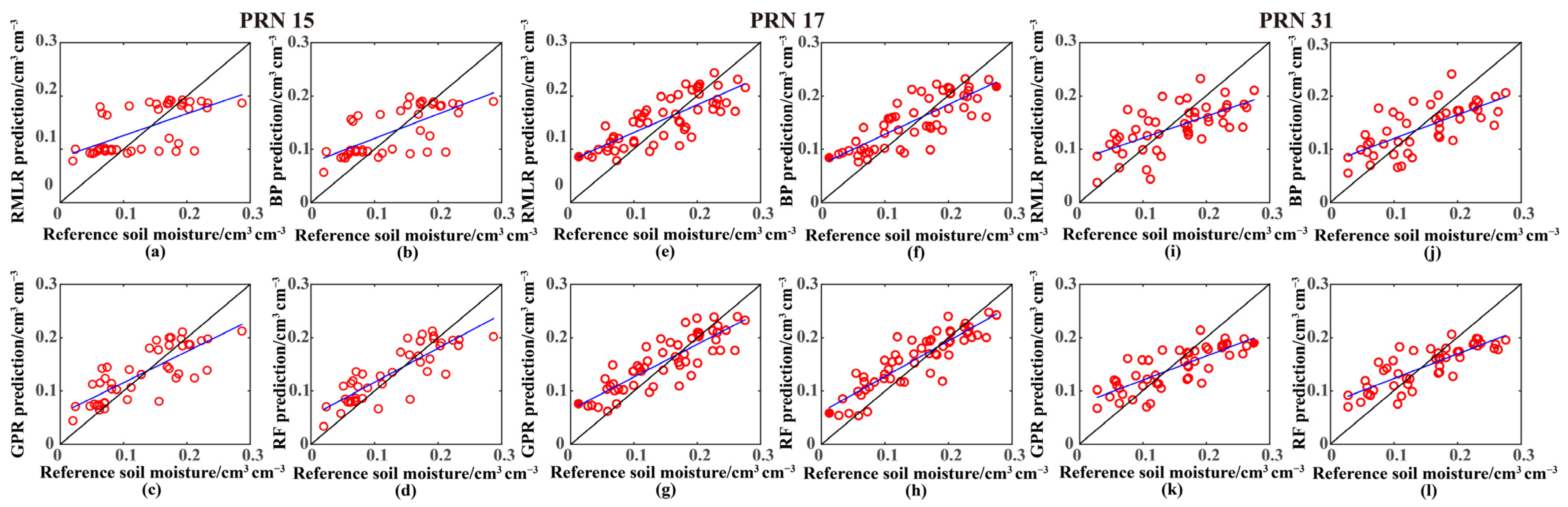
4.3.4. Machine Learning Models Based on Single satellite Data for Soil Moisture Inversion

Based on the MCD robust estimation method and machine learning algorithms, machine learning models for moisture inversion were developed and compared with the robust multiple regression model. The relationship between the predicted and reference soil moisture values of the four models is shown in Figure 10.

From Figure 10, all three machine learning algorithms and the MCD multiple regression method establish a GNSS-IR soil moisture inversion model, and the trend of the predicted soil moisture values of the models is basically consistent with that of the reference values, which illustrates the effectiveness of the method in this manuscript. Although a few predicted values deviate from the reference values, overall, most of the predicted values of the four models fluctuate around the reference value, the RF model has the least deviation, the GPR model has the second lowest deviation, and the BPNN model has the largest deviation, but they all outperform the MCD multiple regression model, proving that machine learning methods may effectively increase the accuracy of GNSS-IR soil moisture inversion.

To further analyze the inversion accuracy of the four models, the R, RMSE, and mean absolute error (MAE) are utilized as the accuracy evaluation criteria. Figure 11 shows the prediction results of the four models for the three GPS satellites. The inversion results of the four models for all visible satellites is shown in Figure 12. The accuracy analysis of the four models for the PRN 15, 17, 31 satellites is shown in Table 5.

Figure 11 and

Table 6. Inversion accuracy of the four models for the different satellites.

Satellite Track	Model	R	RMSE (cm3/cm3)	MAE (cm3/cm3)
PRN 15	RMLR	0.6366	0.0520	0.0424
	BPNN	0.6967	0.0481	0.0390
	GPR	0.7933	0.0409	0.0328
	RF	0.8473	0.0364	0.0297
PRN 17	RMLR	0.7890	0.0438	0.0386
	BPNN	0.8020	0.0420	0.0357
	GPR	0.8491	0.0382	0.0321
	RF	0.8827	0.0354	0.0295
PRN 31	RMLR	0.6168	0.0548	0.0462
	BPNN	0.7065	0.0495	0.0432
	GPR	0.7874	0.0455	0.0386
	RF	0.7995	0.0437	0.0347

show that the R values of the four models established with the three GPS satellite datasets are in the range of 0.63−0.89, and the RMSE and MAE also basically meet the soil moisture inversion accuracy requirements [24]. For the inversion accuracy of the RF model, GPR model, and BPNN model for PRN 15 compared with that of the multiple linear regression model, the R improved by 33.1%, 24.6%, and 9.5%; the RMSE decreased by 30%, 21.3%, and 7.5%; and the MAE decreased by 30%, 22.6%, and 8%, respectively. For the inversion accuracy of the RF model, GPR model, and BPNN model for PRN 17 compared with that of the multiple linear regression model, the R improved by 11.9%, 7.6%, and 1.6%; the RMSE decreased by 19.2%, 12.8%, and 4.2%; and the MAE decreased by 23.6%, 16.8%, and 7.5%, respectively. For the inversion accuracy of the RF model, GPR model, and BPNN model for PRN 31 compared with that of the multiple linear regression model, the R improved by 32.8%, 27.7%, and 14.5%; the RMSE decreased by 21%, 17%, and 9.7%; and the MAE decreased by 19.5%, 16.4%, and 6.5%, respectively. From Figure 12, the R for all satellite tracks increased by 4.3~86.6% compared with the MCD multiple regression model. The RMSE reduced by 2.8~30%. The results show that all three machine learning inversion models outperform the multiple linear regression model in terms of inversion accuracy. The RF model is the most accurate, the GPR model is the second most accurate, and the BPNN model is the least accurate.

4.3.5. Machine Learning Models Based on All Visible Satellites Data for Soil Moisture Inversion

To further verify the generalization ability of the three machine learning models and their recommended parameters, and to enhance the utilization of GNSS data by integrating data from multiple satellites, we developed the all visible satellites model. The process of establishing the all visible satellites model is as follows: To avoid excessive input variables and severe collinearity, we computed the average of the amplitude, frequency, and phase characteristic parameters for each visible satellite for each day. Additionally, to eliminate the influence of dimensional parameters, prevent non-convergence, and facilitate faster modeling, we normalized the three average characteristic parameters as inputs. Soil moisture reference was used as the output to establish a machine learning model. The mean of all normalized satellite data is divided into the test set and training set, and the total model of the P043 station is established by the three machine learning algorithms. The parameter settings of the machine learning algorithms have been verified in previous experiments. The inversion accuracy of the total models is shown in

Table 7. Theoretical background of GNSS-IR soil moisture linear inversion.

Model	R	RMSE (cm3/cm3)	MAE (cm3/cm3)
RMLR	0.6017	0.0551	0.0463
BPNN	0.6346	0.0533	0.0431
GPR	0.6731	0.0493	0.0413
RF	0.7365	0.0387	0.0323

.

Table 7 shows that the four methods are still effective in modeling the soil moisture inversion when all visible satellites data are considered together to build the overall model. It is worth noting that the overall model, although effectively using all satellite data, causes a loss of accuracy. The accuracy of the four methods is similar to the experimental results above, and the machine learning model effectively improves the modeling accuracy, and the RF model has the highest accuracy.

In summary, the machine learning algorithms combined with the MCD robust estimation method can effectively attenuate the influence of environmental factors and observation errors around the GPS station and fully use all reflection signal metrics to improve the soil moisture inversion accuracy.

5. Discussion

The effect of errors in the SNR data has been somewhat neglected in former studies [23]. The SNR data are often smoothed by wavelet decomposition [12,13]. However, the errors in the SNR data are not obvious, and the selection of wavelet decomposition parameters and the reconstruction of the data are not negligible problems. During processing the SNR data to extract the metrics of multipath signal, the error in the SNR is amplified to a certain extent by the nonlinear error propagation and reflected in the metrics. Therefore, we use the MCD robust estimation to deal with the metrics, which effectively avoids some selection problems when using wavelet decomposition. In Figure 3, the experimental results demonstrate that the MCD robust estimation is a reliable method to deal with outliers in the metrics. As shown in Figure 4, the MCD method is significantly better at detecting outliers when the data quality is not high. The comparative study on the quality control of SNR and on the metrics will be described in a subsequent study because it involves the comparison of multiple methods and the selection of parameters, control variables, and other issues.

Each metric of multipath signal carries different surface information. Although the single metric can effectively respond to the changing trend of soil moisture, it does not meet the increasing requirements of the actual soil moisture monitoring accuracy. Meanwhile, the linearized modeling does not consider the contribution of each metric to the inverse soil moisture in an integrated manner. As shown in Table 1, the inversion accuracy of the multiple regression model based on the MCD method is significantly better than those of the univariate regression models.

Although machine learning algorithm has been applied to GNSS-IR surface parameter inversion, there are few studies on soil moisture. In addition, the machine learning algorithm itself has certain uncertainty and requires some parameters to be set. Different parameter settings will affect the modeling accuracy of the machine learning algorithm. If the optimization algorithm is used to identify the ideal parameters of the machine learning algorithm, the uncertainty caused by the optimization algorithm will also have an impact on the model accuracy to some extent. The optimization algorithm combined with the machine learning algorithm will also cause a huge computational cost, especially when the amount of data is large. In this manuscript, we systematically study the parameter selection, inversion accuracy, and generalization capability of BPNN, GPR, and RF machine learning algorithms. The optimal parameters combinations for the three machine learning algorithms to construct robust multivariate GNSS-IR soil moisture inversion models are given experimentally. These parameters have strong generalization ability, which fills the gap of difficult parameter selection when constructing GNSS-IR soil moisture inversion models with machine learning algorithms. Figure 12 shows that machine learning-based multivariate nonlinear models further enhance the accuracy of soil moisture inversion. Differences in satellite signal quality may be the reason why the total model accuracy is not as good as some single satellite models.

6. Conclusions

Overall, this study mainly addresses the following problems in GNSS-IR soil moisture inversion modeling: observation errors, insufficient utilization of multipath signal information, and the difficulty in integrating environmental factors such as ground roughness and vegetation cover. The minimum covariance determinant (MCD) robust estimation method is introduced, and on this basis, three machine learning algorithms—the back propagation neural network (BPNN), Gaussian process regression (GPR), and random forest (RF)—are taken into consideration to establish nonlinear GNSS-IR soil moisture inversion models with single satellite data and all satellite data, respectively, and the optimal parameters combinations for the three machine learning algorithms is provided by experiment. The following conclusions are drawn.

① Compared with the traditional methods, the MCD method has a stronger detection effect and can effectively enhance the accuracy of GNSS-IR soil moisture inversion.

② The accuracy of soil moisture inversion can be improved by considering the frequency, amplitude, and phase of the multipath signals simultaneously.

③ Compared with the robust multiple linear regression model, machine learning algorithms can further enhance the modeling accuracy. The RF model has the highest inversion accuracy, and the R of all satellite tracks are 4.3~86.6% higher than those of the robust multiple linear regression model. The RMSE are 2.8~30% lower than those of the robust multiple linear regression model.

④ The RF algorithm is the best choice for constructing a robust multivariate GNSS-IR soil moisture model. Its parameter selection is more fixed which represents a strong generalization capability. The recommended decision tree and the number of nodes for the RF algorithm are 80 and 1. The inversion results of the GPR algorithm is slightly less accurate, but the kernel function ‘Ard exponential kernel’ is a relatively fixed choice for the GPR algorithm. The activation function of the BPNN algorithm is relatively fixed, but the selection of the number of hidden layers will slightly affect the inversion accuracy, so the BPNN algorithm is not recommended.

⑤ Compared with the single satellite model, the total model using all satellite data has more generalization ability but causes some loss of accuracy.

The results show that the machine learning algorithms fused with the MCD method can effectively simplify GNSS-IR soil moisture inversion modeling, reduce the influence of observation errors, improve the accuracy of soil moisture inversion, and have strong generalization ability. However, the effects of surface roughness, vegetation, and soil temperature on the soil moisture inversion model were not quantified in this study. The effects of environmental factors at different stations can be further quantitatively evaluated using machine learning algorithms with multi-satellite and multifrequency observations. In addition, the adaptive selection and applicability evaluation of parameters for machine learning algorithms need to be further investigated when modeling the GNSS-IR soil moisture inversion model. The integration of high-precision ground-based GNSS-IR soil moisture data and large-scale satellite-based soil moisture data can generate high-precision and high-spatial-temporal-resolution soil moisture products, which have great potential to provide decision-making support for sustainability and environmental management.

References

1. Saux-Picart, S.; Ottlé, C.; Decharme, B.; André, C.; Zribi, M.; Perrier, A.; Coudert, B.; Boulain, N.; Cappelaere, B.; Descroix, L.; et al. Water and Energy Budgets Simulation over the AMMA-Niger Super-Site Spatially Constrained with Remote Sensing Data. J. Hydrol. 2009, 1, 287–295. [Google Scholar] [CrossRef]
2. Blöschl, G.; Bierkens, M.F.; Chambel, A.; Cudennec, C.; Destouni, G.; Fiori, A.; Kirchner, J.W.; McDonnell, J.J.; Savenije, H.H.; Sivapalan, M.; et al. Twenty-three unsolved problems in hydrology (UPH)—A community perspective. Hydrol. Sci. J. 2019, 64, 1141–1158. [Google Scholar] [CrossRef]
3. Zhang, D.J.; Zhan, J.; Qiao, Z.; Zupan, R. Evaluation of the Performance of the Integration of Remote Sensing and Noah Hydrologic Model for Soil Moisture Estimation in Hetao Irrigation Region of Inner Mongolia. Can. J. Remote Sens. 2020, 46, 552–566. [Google Scholar] [CrossRef]
4. Albergel, C.; De Rosnay, P.; Gruhier, C.; Munoz-Sabater, J.; Hasenauer, S.; Isaksen, L.; Kerr, Y.; Wagner, W. Evaluation of remotely sensed and modelled soil moisture products using global ground-based in situ observations. Remote Sens. Environ. 2012, 118, 215–226. [Google Scholar] [CrossRef]
5. Kerr, Y.H.; Waldteufel, P.; Wigneron, J.-P.; Martinuzzi, J.; Font, J.; Berger, M. Soil moisture retrieval from space: The Soil Moisture and Ocean Salinity (SMOS) mission. IEEE Trans. Geosci. Remote Sens. 2001, 39, 1729–1735. [Google Scholar] [CrossRef]
6. Chew, C.C.; Small, E.E. Soil Moisture Sensing Using Spaceborne GNSS Reflections: Comparison of CYGNSS Reflectivity to SMAP Soil Moisture. Geophys. Res. Lett. 2018, 45, 4049–4057. [Google Scholar] [CrossRef]
7. Li, X.; Yang, D.; Yang, J.; Zheng, G.; Han, G.; Nan, Y.; Li, W. Analysis of coastal wind speed retrieval from CYGNSS mission using artificial neural network. Remote Sens. Environ. 2021, 260, 112454. [Google Scholar] [CrossRef]
8. Zavorotny, V.U.; Gleason, S.; Cardellach, E.; Camps, A. Tutorial on Remote Sensing Using GNSS Bistatic Radar of Opportunity. IEEE Geosci. Remote Sens. Mag. 2014, 2, 8–45. [Google Scholar] [CrossRef]
9. Wu, X.; Ma, W.; Xia, J.; Bai, W.; Jin, S.; Calabia, A. Spaceborne GNSS-R Soil Moisture Retrieval: Status, Development Opportunities, and Challenges. Remote Sens. 2020, 13, 45. [Google Scholar] [CrossRef]
10. Yu, K. Navigation Satellite Constellations and Navigation Signals. In Theory and Practice of GNSS Reflectometry; Springer: Singapore, 2021; pp. 13–34. [Google Scholar]
11. Hall, C.D.; Cordey, R.A. Multistatic scatterometry. In Proceedings of the International Geoscience and Remote Sensing Symposium, ‘Remote Sensing: Moving Toward the 21st Century’, Edinburgh, UK, 12–16 September 1988; Volume 1, pp. 561–562. [Google Scholar]
12. Bilich, A.; Larson, K.M. Mapping the GPS multipath environment using the signal-to-noise ratio (SNR). Radio Sci. 2007, 42, 1–16, Erratum in Radio Sci. 2008, 43, 1. [Google Scholar] [CrossRef]
13. Bilich, A.; Larson, K.M.; Axelrad, P. Modeling GPS phase multipath with SNR: Case study from the Salar de Uyuni, Boliva. J. Geophys. Res. Solid Earth 2008, 113, 4. [Google Scholar]
14. Kavak, A.; Vogel, W.J.; Xu, G. Using GPS to measure ground complex permittivity. Electron. Lett. 1998, 34, 254–255. [Google Scholar] [CrossRef]
15. Larson, K.M.; Small, E.E.; Gutmann, E.; Bilich, A.; Axelrad, P.; Braun, J. Using GPS multipath to measure soil moisture fluctuations: Initial results. GPS Solut. 2008, 12, 173–177. [Google Scholar] [CrossRef]
16. Larson, K.M.; Small, E.E.; Gutmann, E.D.; Bilich, A.L.; Braun, J.J.; Zavorotny, V.U. Use of GPS receivers as a soil moisture network for water cycle studies. Geophys. Res. Lett. 2008, 35, 24. [Google Scholar] [CrossRef]
17. Larson, K.M.; Braun, J.J.; Small, E.E.; Zavorotny, V.U.; Gutmann, E.D.; Bilich, A.L. GPS Multipath and Its Relation to Near-Surface Soil Moisture Content. IEEE J. Sel. Top. Appl. Earth Observ. Remote Sens. 2010, 3, 91–99. [Google Scholar] [CrossRef]
18. Chew, C.; Small, E.E.; Larson, K.M. An algorithm for soil moisture estimation using GPS-interferometric reflectometry for bare and vegetated soil. GPS Solut. 2016, 20, 525–537. [Google Scholar] [CrossRef]
19. Roussel, N.; Frappart, F.; Ramillien, G.; Darrozes, J.; Baup, F.; Lestarquit, L.; Ha, M.C. Detection of Soil Moisture Variations Using GPS and GLONASS SNR Data for Elevation Angles Ranging from 2° to 70°. IEEE J. Sel. Top. Appl. Earth Observ. Remote Sens. 2016, 9, 4781–4794. [Google Scholar] [CrossRef]
20. Vey, S.; Güntner, A.; Wickert, J.; Blume, T.; Ramatschi, M. Long-term soil moisture dynamics derived from GNSS interferometric reflectometry: A case study for Sutherland, South Africa. GPS Solut. 2016, 20, 641–654. [Google Scholar] [CrossRef]
21. Chew, C.C.; Small, E.E.; Larson, K.M.; Zavorotny, V.U. Vegetation Sensing Using GPS-Interferometric Reflectometry: Theoretical Effects of Canopy Parameters on Signal-to-Noise Ratio Data. IEEE Trans. Geosci. Remote Sens. 2015, 53, 2755–2764. [Google Scholar] [CrossRef]
22. Wan, W.; Larson, K.M.; Small, E.E.; Chew, C.C.; Braun, J.J. Using geodetic GPS receivers to measure vegetation water content. GPS Solut. 2015, 19, 237–248. [Google Scholar] [CrossRef]
23. Wang, X.; Zhang, Q.; Zhang, S. Water levels measured with SNR using wavelet decomposition and Lomb–Scargle periodogram. GPS Solut. 2018, 22, 22. [Google Scholar] [CrossRef]
24. Small, E.E.; Larson, K.M.; Chew, C.C.; Dong, J.; Ochsner, T.E. Validation of GPS-IR Soil Moisture Retrievals: Comparison of Different Algorithms to Remove Vegetation Effects. IEEE J. Sel. Top. Appl. Earth Observ. Remote Sens. 2016, 9, 4759–4770. [Google Scholar]
25. Neelam, M.; Colliander, A.; Mohanty, B.P.; Cosh, M.H.; Misra, S.; Jackson, T.J. Multiscale Surface Roughness for Improved Soil Moisture Estimation. IEEE Trans. Geosci. Remote Sens. 2020, 58, 5264–5276. [Google Scholar]
26. Herbert, C.; Camps, A.; Wellmann, F.; Vall-Llossera, M. Bayesian Unsupervised Machine Learning Approach to Segment Arctic Sea Ice Using SMOS Data. Geophys. Res. Lett. 2021, 48, 6. [Google Scholar] [CrossRef]
27. Jia, Y.; Jin, S.; Savi, P.; Gao, Y.; Tang, J.; Chen, Y.; Li, W. GNSS-R soil moisture retrieval based on a XGboost machine learning aided method: Performance and validation. Remote Sens. 2019, 11, 1655. [Google Scholar] [CrossRef]
28. Senyurek, V.; Lei, F.; Boyd, D.; Gurbuz, A.C.; Kurum, M.; Moorhead, R. Evaluations of Machine Learning-Based CYGNSS Soil Moisture Estimates against SMAP Observations. Remote Sens. 2020, 12, 3503. [Google Scholar] [CrossRef]
29. Senyurek, V.; Lei, F.; Boyd, D.; Kurum, M.; Gurbuz, A.C.; Moorhead, R. Machine Learning-Based CYGNSS Soil Moisture Estimates over ISMN sites in CONUS. Remote Sens. 2020, 12, 1168. [Google Scholar] [CrossRef]
30. Ren, C.; Liang, Y.J.; Lu, X.J.; Yan, H.B. Research on the soil moisture sliding estimation method using the LS-SVM based on multi-satellite fusion. Int. J. Remote Sens. 2019, 40, 2104–2119. [Google Scholar] [CrossRef]
31. Larson, K.M.; Small, E.E. Normalized Microwave Reflection Index: A Vegetation Measurement Derived from GPS Networks. IEEE J. Sel. Top. Appl. Earth Observ. Remote Sens. 2014, 7, 1501–1511. [Google Scholar] [CrossRef]
32. Martín, A.; Anquela, A.B.; Ibáñez, S.; Baixauli, C.; Blanc, S. Python software to transform GPS SNR wave phases to volumetric water content. GPS Solut. 2022, 26, 7. [Google Scholar] [CrossRef]
33. Larson, K.M.; Nievinski, F.G. GPS snow sensing: Results from the EarthScope Plate Boundary Observatory. GPS Solut. 2013, 17, 41–52. [Google Scholar] [CrossRef]
34. Chen, K.; Cao, X.; Shen, F.; Ge, Y. An Improved Method of Soil Moisture Retrieval Using Multi-Frequency SNR Data. Remote Sens. 2021, 13, 3725. [Google Scholar] [CrossRef]
35. Liang, Y.J.; Ren, C.; Wang, H.Y.; Huang, Y.B.; Zheng, Z.T. Research on soil moisture inversion method based on GA-BP neural network model. Int. J. Remote Sens. 2019, 40, 2087–2103. [Google Scholar] [CrossRef]
36. Lv, J.; Zhang, R.; Tu, J.; Liao, M.; Pang, J.; Yu, B.; Li, K.; Xiang, W.; Fu, Y.; Liu, G. A GNSS-IR Method for Retrieving Soil Moisture Content from Integrated Multi-Satellite Data That Accounts for the Impact of Vegetation Moisture Content. Remote Sens. 2021, 13, 2442. [Google Scholar] [CrossRef]
37. Hubert, M.; Debruyne, M.; Rousseeuw, P.J. Minimum covariance determinant and extensions. Wires Comput. Stat. 2018, 10, 1421. [Google Scholar] [CrossRef]
38. Rumelhart, D.E.; Hinton, G.E.; Williams, R.J. Learning representations by back-propagating errors. Nature 1986, 323, 533–536. [Google Scholar] [CrossRef]
39. Wythoff, B.J. Backpropagation neural networks. A tutorial. Chemom. Intell. Lab. 1993, 18, 115–155. [Google Scholar] [CrossRef]
40. Rasmussen, C.E. Gaussian Processes in Machine Learning; Advanced Lectures on Machine Learning; Springer: Berlin/Heidelberg, Germany, 2004; pp. 63–71. [Google Scholar]
41. Breiman, L. Random forests. Mach. Learn. 2001, 45, 5–32. [Google Scholar] [CrossRef]
42. Jia, Y.; Jin, S.; Savi, P.; Yan, Q.; Li, W. Modeling and Theoretical Analysis of GNSS-R Soil Moisture Retrieval Based on the Random Forest and Support Vector Machine Learning Approach. Remote Sens. 2020, 12, 3679. [Google Scholar] [CrossRef]
Figure 1. (a) Location of P043. (b) The surrounding environment of P043 (https://gnss-h2o.jpl.nasa.gov/index.php, accessed on 1 December 2020).
Sustainability 15 06919 g001
Figure 2. The framework and experimental design of the proposed GNSS-IR soil moisture inversion algorithms integrating robust estimation with machine learning.
Sustainability 15 06919 g002
Figure 3. Outlier detection results of the triple standard deviation method and the MCD method for all satellites.
Sustainability 15 06919 g003
Figure 4. Outlier detection results of the multipath signal metrics time series for PRN 17. (a) Amplitude results of the triple standard deviation method. (b) Amplitude results of the MCD method. (c) Frequency results of the triple standard deviation method. (d) Frequency results of the MCD method. (e) Phase results of the triple standard deviation method. (f) Phase results of the MCD method.
Sustainability 15 06919 g004
Figure 5. Comparison of the noise reduction effects of the two robust estimation methods. ‘Amplitude MCD’ denotes the RMSE of the linear model established with the amplitude time series denoised by using the MCD method. ‘TSD’ stands for the triple standard deviation method.
Sustainability 15 06919 g005
Figure 6. Root mean square error of the four robust linear models for all visible satellites.
Sustainability 15 06919 g006
Figure 7. The inversion results of BPNN models. (a) The inversion results of all visible satellites with different number of hidden layers. (b) The inversion results of all visible satellites with three activation functions.
Sustainability 15 06919 g007
Figure 8. The inversion results of GPR models. (a) The inversion results of all visible satellites with the ARD exponential kernel function. (b) The inversion results of all visible satellites with three kernel functions.
Sustainability 15 06919 g008
Figure 9. The inversion results of RF models. (a) Inversion results of the different numbers of decision trees for the RF model. (b) The inversion results of all visible satellites with 80 decision trees and 1 node.
Sustainability 15 06919 g009
Figure 10. Comparison of the soil moisture predicted by the four models and their reference values. (a) Results of the PRN 15. (b) Results of the PRN 17. (c) Results of the PRN 31.
Sustainability 15 06919 g010
Figure 11. Results of the four models for the PRN 15, 17, 31 satellites. The blue line represents the performance of different model and the black line the ideal 1:1 line. Subplots (ad) are the results of the PRN 15. Subplots (eh) are the results of the PRN 17. Subplots (il) are the results of the PRN 31.
Sustainability 15 06919 g011
Figure 12. The inversion results of the four models for all visible satellites.
Sustainability 15 06919 g012