Machine Learning-Based Tap Temperature Prediction and Control for Optimized Power Consumption in Stainless Electric Arc Furnaces (EAF) of Steel Plants

Abstract

The steel industry has been forced to switch from the traditional blast furnace to the electric arc furnace (EAF) process to reduce carbon emissions. However, EAF still relies entirely on the operators’ proficiency to determine the electrical power input. This study aims to enhance the efficiency of the EAF process by predicting the tap temperature in real time through a data-driven approach and by applying a system that automatically sets the input amount of power to the production site. We developed a tap temperature prediction model (TTPM) with a machine learning (ML)-based support vector regression (SVR) algorithm. The operation data of the stainless EAF, where the actual production work was carried out, were extracted, and the models using six ML algorithms were trained. The model validation results show that the model with an SVR radial basis function (RBF) algorithm resulted in the best performance with a root mean square error (RMSE) of 20.14. The SVR algorithm performed better than the others for features such as noise. As a result of a five-month analysis of the operating performance of the developed TTPM for the stainless EAF, the tap temperature deviation decreased by 17% and the average power consumption decreased by 282 kWh/heat compared with the operation that depended on the operator’s skill. In the results of the economic evaluation of the facility investment, the economic feasibility was found to be sufficient, with an internal rate of return (IRR) of 35.8%. Applying the developed TTPM to the stainless EAF and successfully operating it for ten months verified the system’s reliability. In terms of the increasing proportion of EAF production used to decarbonize the steel industry, it is expected that various studies will be conducted more actively to improve the efficiency of the EAF process in the future. This study contributes to the improvement of steel companies’ manufacturing competitiveness and the carbon neutrality of the steel industry by achieving the energy and production efficiency improvements associated with the EAF process.

1. Introduction

1.1. Background of Study

In 2015, the Paris Climate Agreement was established to reduce greenhouse gases and prevent global warming, declaring a long-term international goal of suppressing global average temperature rises to below 2 °C and trying not to exceed 1.5 °C [1]. Carbon dioxide emissions must be reduced by more than 45% by 2030 compared with 2010, and global carbon neutrality is to be achieved by 2050 [2]. With the goal of 2050 carbon neutrality, many countries, including developed countries, such as those of the European Union (EU), the US, and Japan, have set nationally determined contributions (NDC) suitable for each country’s situation. Carbon neutrality at the national level is important for responding to climate change and suppressing the increase in the earth’s average temperature in the future. International standards, such as carbon neutrality and climate response, strengthening environmental requirements for clients, and rising carbon emission prices, are rapidly changing. The steel industry, which accounts for 7% of total industrial carbon dioxide emissions and 8% of energy consumption, is facing increasing demands from clients for low-carbon steel, such as scrap, and eco-friendly energy. Accordingly, a new technical approach is needed to transform the process paradigm beyond the carbon-based furnace [3,4]. Various technologies have been attracting attention as reducing carbon in the steel industry. Among these, the electric arc furnace (EAF) process using direct reduced iron (DRI) or completely reduced scrap has received particular attention. An EAF with DRI uses raw steel materials that has had some carbon removed prior to its processing instead of using the traditional blast furnace process. As a result, it has the advantage of lower carbon emissions. Accordingly, the proportion of EAF process production is expected to increase. Technical progress and continuous research of electric furnace processes are required to secure competitiveness [5].

Company P, a Korean steel maker, produces steel products at two integrated steelworks, with a total crude steel production of 40 million tons and a stainless-steel production of two million tons. Company P has two EAFs, each of which are stainless steel [6]. This study mainly aimed to improve the productivity of stainless-steel Type B EAF, an alternating current type EAF used by Company P. After the raw material is loaded, the operator inputs the amount of electrical power to be put into the charge (Ch’), via the power schedule setting screen of the human–machine interface (HMI) in the operating room, prior to the melting operation. HMI is a computer system for controlling the processes at a steel plant site. The HMI screen displays various elements that operators can manipulate, such as facility diagrams, input buttons, texts, numbers, input fields, alarm pop-ups, and more.

The overall operation schedule is automatically controlled based on this process. In the situation of an EAF operation, any measuring device to measure the operation status cannot be placed inside the furnace because a high-voltage current over 500 V and 40 kA is energized through the electrode. Therefore, the operator refers to the operating conditions, such as raw material input components, input amount, and previous Ch’ operation results, to determine the required electrical power input before the operation starts through subjective prediction based on their operational experience. The working guideline of Company P specifies that the operator should make power supply decisions based on their empirical judgment and the current site situation. However, this dependence on the individual operator’s subjective judgment causes the operation quality to fluctuate according to the operator’s capability, resulting in inefficiencies of the process.

This study developed an EAF tap temperature prediction model (TTPM) and an AI automatic operation system based on machine learning (ML) to solve these problems. TTPM was developed to predict tap temperature in real time using only those features that can be secured during operation, thus ensuring that it can be applied to an EAF site where actual production work is performed. In addition, an AI automatic operation system was developed to automatically control the operation, without the intervention of an operator, based on the tapping temperature predicted by TTPM. The developed system is currently still being applied to the field production site to assist in its operation. It will be a reference for other studies in that the effects of reduced power consumption and fixed costs have been verified.

The overall composition and details of this study are as follows. The introduction consists of Section 1,Section 2,Section 3. Section 1 describes the background and necessity of the study, derives improvement opportunities according to the current EAF operation method and explains the study’s goal. Section 2 reviews previous studies, examining the trends of ML research targeting the steel industry and their differences with this study. In Section 3, the problems of the existing EAF operation methods are derived, and the research methodology is discussed. Section 4,Section 5,Section 6 are the cores of this paper; Section 4 explains the data collection and preprocessing method, and Section 5 describes the theoretical background of the ML algorithm, model training, the developed model’s verification, performance evaluation, and the procedure for selecting the optimal model by TTPM. Section 6 explains the developed model’s field application, system configuration, and the development method of the tapping temperature prediction system (TTPS) and analyzes the developed TTPS field application results. Section 6 summarizes the issues to be discussed in future research and the overall findings.

1.2. Literature Review

Previous studies have been reviewed in consideration of two aspects. First, with regard to the application of ML technology in the steel industry, various studies were investigated with keywords combining ML, AI, and terms related to the steel process. Second, the authors reviewed prior studies that applied ML technology to EAF and collected literature using keywords combining EAF, arc furnace, tap temperature, and ML or AI. Through this, the authors reviewed the approaches of similar research models and explored their limits.

1.2.1. Machine Learning Application in the Steel Industry

Previous studies that applied ML technology in the steel industry were reviewed. There were a number of studies on the prediction of iron ore prices using the ML technique. Lee et al. [7] developed a prediction model for Chinese iron ore prices by applying the long short-term memory (LSTM) algorithm. Their model used the volumes of steel exported from Korea, China, and Japan; the demand and supply volumes of Chinese steel; and scrap raw material prices as the variables. Their model’s mean absolute percent error (MAPE) was 5.96%. Most of the studies that applied ML were related to the steel manufacturing process. Liu et al. [8] studied a support vector machine (SVM)-based model that determines whether the operation is abnormal through the interpretation of 14 factors and 1600 training data that were obtained via measurements taken during the operation of the blast furnace. They also verified its feasibility and effectiveness with 800 test data. Liu et al. [9] developed a model for calculating the optimal raw material mixing ratio in the sintering process and applied it to actual operation to verify the effect of reducing raw material costs by 4.63 USD/ton (3.8%).

Predicting a precise endpoint of the converter process to remove impurities from pig iron is vital for productivity and quality. Jo et al. [10] predicted the oxygen-blowing amount, which is a factor that determines the endpoint, using existing operation data. Schlueter et al. [11] produced the data by attaching a sensor to measure off-gas composition and used these data for training. Bae et al. [12] sought to predict the final temperature and composition ratio of carbon and phosphorus under current operating conditions. Tian et al. [13] developed a hybrid model that predicted the optimal parameters of the thermal model previously used in the ladle furnace (LF) process. They improved the prediction performance within ±5 °C of the temperature deviation of molten steel. Laha et al. [14] developed a crude steel yield prediction model using random forest (RF), artificial neural network (ANN), and support vector regression (SVR) algorithms. They verified that SVR performed better than RF and ANN algorithms. Santos et al. [15] calculated the distance between the operation data of 645 regular products and 244 defective products to determine whether or not the ultra-tensile strength products were from the iron casting process. They achieved a detection success rate of 78%. Previous studies seeking to predict the clogging of a submerged entry nozzle (SEN), a chronic problem in the continuous casting process, were also reviewed. Wang et al. [16] developed an LSTM model that detects the time series change of the clogging index data for three minutes using the calculation method presented in previous studies. The clogging index after 36 s was predicted, and the coefficient of determination performance was 0.971.

Several studies were found on the application of ML to the prediction of strip quality in the rolling process. Ghorai et al. [17] developed an image recognition model capable of detecting 24 defects in real time by training 1432 strip surface images taken in hot rolling processes. However, their model worked only at 5 m/second or less and under an ideal environment without vibration and noise. Ding et al. [18] predicted the camber of the product caused by the asymmetry of the roll pressing control in the plate process based on SVM. They also conducted a study wherein they were able to control camber generation within ±6% in conjunction with roll tilt controls.

Studies on the application of AI and ML technologies for digitalization and carbon emission reduction in the steel industry were also reviewed. Colla et al. [19] proposed various ML models and theories for digitalization that can improve carbon neutrality in steel manufacturing processes by using AI and ML technologies. However, their study was limited due to the absence of an attempt to apply their results to an actual industrial site. Stavropoulos et al. [20] developed a framework utilizing big data techniques to reduce carbon dioxide emissions in the steel manufacturing industry. Their study proposed different metrics from the perspectives of carbon emissions and cost. Zhou et al. [21] suggested optimizing manufacturing processes using simulation, visualization, and ML for digitalization in the manufacturing industry.

1.2.2. Machine Learning Model for Electric Arc Furnace

Previous studies that applied ML to the EAF process were reviewed. The literature review results regarding the prediction of the amount of power input are discussed in this section. Reimann et al. [22] developed a model applying three ML algorithms, including an artificial neural network (ANN), using over 21,000 operational data extracted from five EAF locations. As a result of the performance evaluation, the gaussian process regression (GPR) model performed best among the three ML algorithms. Their newly developed model was superior to the empirical (Köhle) model. However, their study had a limitation as it was only a theoretical study and it was thus difficult to use in actual operation through the application of a tapping amount factor that could not be obtained. In addition, several studies have used factors that cannot be obtained during operation. Kovačič et al. [23] developed a model by training 25 factors, such as input raw material information and operation waiting time. However, there was a limitation in that, due to the subjective intervention of the operator, unoptimized power input performance data were involved. Carlsson et al. [24] conducted a theoretical study on whether an operation can be statistically modeled using the tap-to-tap time (T-T) and discharging time of molten steel. However, it was similarly limited in its application to the actual operation site.

The prior studies on EAF tap temperature prediction are as follows. Li et al. [25] developed a model that predicts tapping temperature with 95% accuracy within ±20 °C by applying LSTM. However, it was unclear what factors were used and whether predictions could be made in real time by applying them to actual operations. Blažič et al. [26] sought to predict the molten metal temperature in real time during the melting operation. However, electricity supply must be stopped, and the roof must be opened to measure the molten metal temperature during operation. This means that the study suffered from a limitation wherein production time delays of longer than 1 min occur. As a result, their approach cannot be applied to an actual EAF process because productivity and power efficiency would be seriously degraded.

As a result of reviewing the previous studies above, it was found that various studies that applied ML technology to the steel industry were implemented under the rapid development of ML applications and computing power. The authors focused on the studies that applied ML or deep learning (DL) techniques to accumulate operation data regarding the prediction of electrical power input or the tap temperature of EAF, which are closely related to this study. Firstly, the electric power input is a factor that includes the operator’s subjective judgment. Therefore, it is possible to imitate the inefficient operator’s manual operation when an ML model is trained with the existing data. Accordingly, this study aimed to predict the tapping temperature, which is an objective indicator. Previous studies that did not produce satisfactory performance were benchmarked, though less than ten factors were used, and the maximum achievable factors were secured and applied to model development. Because this study aimed to develop a sustainable system that can be applied to actual EAF sites even after the research is complete, the model was developed using only features that can be ensured during operation.

Moreover, the operator’s workload was reduced by developing an AI operation system that automatically controls the operation based on the tap temperature predicted by TTPM and applying it to the site. The system that was developed as a result of this study verified the effect of a reduction in electrical power and costs by analyzing the operational data for 49 days during a field application test of five months. In addition, it can be differentiated from other studies in that it can be applied to the actual production site and assist the operator.

2. Problem Statements and Model Development

2.1. Problems of Electric Arc Furnace Operation

This study analyzed the electrical power input results among the operation data for 4598 Ch’ produced from February to September 2021 from the operation DB stored in the process computer (PC) of Company P’s stainless steel Type B EAF. Although the facility installed on the site can precisely control the electrical power input in units of 50 kWh, the operator conventionally adjusts the electrical power input at 500-kWh increments during operation [6]. Figure 1 shows the electrical power input described above, and the X-axis represents the amount of electrical power used to produce molten metal. The Y-axis represents the number of Ch’. The value of the Y-axis exists at a high frequency every 500 kWh of the X-axis in Figure 1.

Next, the tap temperature data for steel type 304, which has the highest production share from February to September 2021, were examined. The tapping temperature data generally showed a normal distribution with a temperature distribution of 1420~1740 °C. According to Company P’s work standards, the management standards were established so that the tap temperature of the EAF was aimed at 1580 ± 20 °C [6]. As a result of calculating the hit rate for tapping within the tap temperature range of the management standard, only 1715 Ch’ out of steel type 304’s total of 3105 Ch’ produced during the period satisfied the tap temperature management standard. Hence, the hit rate of tap temperature showed an insufficient result of 55.2%. The remaining 1390 Ch’, which accounted for 44.8%, did not meet the operation management standards, and cases where the tap temperature standard range was exceeded by more than two fold (404 °C or more) occupied 16.8% with 519 Ch’. Additionally, the average tap temperature was 1570.14 °C, which is 9.94 °C lower than the target tap temperature, and the standard deviation was 31.4 °C, which was a significant value compared with the management standard deviation of ±20 °C. The power input and tap temperature data examined above directly show the inefficiency of the current EAF operation. Accordingly, it was possible to indirectly predict that it would have a negative impact on production costs in terms of energy consumption and production time.

Figure 2 illustrates the tap temperature of steel type 304 described above as the X-axis and the number of Ch’ as the Y-axis.

Table 1. The heat counts of tap temperature deviation in EAF for steel type 304 (February to September 2021).

Deviation of Tap Temp.	Count (Heats)	Rate (%)
±0~20 °C	1715	55.2
±21~40 °C	871	28.0
±41 °C~	519	16.8
Total	3105	100

lists the calculation results of the tap temperature hit rate.

As discussed above, the current EAF is operated with the electrical power input based on subjective judgment and prediction by the operator. Problems this can cause include, firstly, the electrical power input deviation that occurs depending on the operator’s experience and skill level; and secondly, the impossibility of fine-tuning the tap temperature that derives from the practice of setting the electrical power input in units of 500 kWh. For this reason, excessive thermal energy is supplied to hit the molten metal to a high temperature when electrical power is over-input. Therefore, productivity decreases, electrical power costs increase, electrode consumption increases due to an increase in tap-to-tap time (T-T), and refractory wear increases due to hit load [27,28]. In addition, if the molten steel inside the EAF is maintained at a high temperature for a long time at a level that exceeds the cooling system’s capacity, there is a possibility of steam leakage due to damage to the cooling structure [29]. Conversely, when the proper temperature of the molten metal cannot be maintained due to insufficient electrical power input, undissolved residual scrap is generated inside the EAF, which impairs the consistency of the next Ch’ operation. In addition, ferroalloy is added to supplement the weight of molten steel produced during the argon oxygen decarburization (AOD) operation, which is a post-operation process, and heating materials such as FeSi are added to secure the temperature, adversely affecting productivity and cost [30].

2.2. Model Development

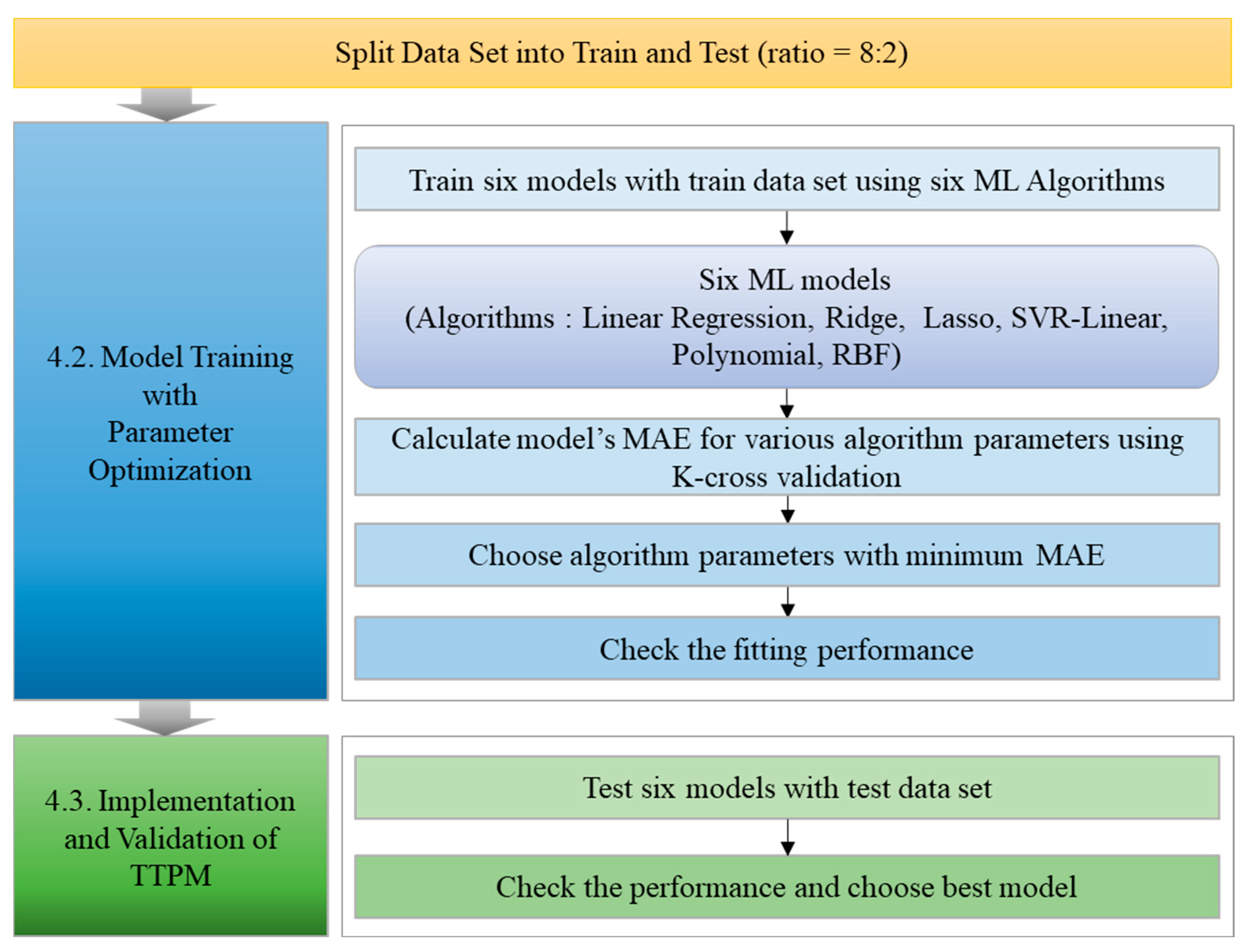
Operational data such as weight, temperature, time, and electrical variables required to develop the model were extracted from the PC and pre-processed to develop the training dataset. Details about this are discussed in Section 4. Next, the data were divided into a training (80%) and a test (20%) dataset by random sampling in the model development stage. Six ML algorithms—linear regression, ridge, lasso, SVR-linear, polynomial and radial basis function (RBF)—were trained with a training dataset. At this time, the model parameters were optimized by k-fold cross-validation to prevent overfitting. After that, the error function of the model was calculated with the test dataset to check the model’s performance, and then TTPM for the optimal tapping temperature prediction was selected. This process is discussed in detail in Section 5. The predictive performance was evaluated by comparing the standard deviation of the tapping temperature of the operation results when the AI automatic function was turned off during the site test with the operation performance when it was turned on. The economic effect was compared in terms of power cost and production by calculating the amount of power input set by the operator and the amount of power input the existing system could save. Section 6 describes the system development process, including hardware and software and field application plans, and then discusses the performance of TTPM, improvement effects, and implications analyzed as a result of site application. The detailed procedure for model development in this study is shown in Figure 3.

3. Data Preparation

EAF operational data were collected for this study. Because operational data are collected at each operation stage of the EAF, it is first necessary to explain the EAF operation process. In EAF, a high-current arc is energized to scrape through a carbon-component electrode fixed to an electrode arm, and the raw material is heated and melted with arc thermal energy [31]. As the dissolution progresses, the arc is maintained in synchronization with the lowering height of the raw material, and the electrode arm cylinder (hydraulic electrode elevating device) moves up and down to adjust the gap between the raw material and the electrode to input power efficiently. The gap between the raw material and the electrode acts as a resistance, which determines the arc’s current. The current balance between the three phases and the power input speed according to the operation stage is adjusted. In addition, as the voltage can be changed without downtime even though power is being applied through the on-line tap changer (OLTC) installed in the transformer, the voltage is differentiated according to the operating stage and scrap melting situation to input power efficiently.

The general EAF operation sequence and its purpose is explained step by step as follows. The raw material charging operation is the operation of inputting the raw material according to the required components of the molten metal in an optimal schedule. The melting operation aims to produce stable tapping components and tapping amounts through a rapid and efficient dissolution of raw materials. Scrap used as the primary raw material is solid with an unspecified shape, and the volume decreases sharply during dissolution. As a result it is generally the case that, after the raw materials charging and melting process is performed twice, the heating operation, which is the final melting task of adjusting the tapping temperature with low voltage and short arc, is performed. In addition, oxygen is also injected as an auxiliary heat source into a pipe-shaped lance through a front work tool across the secondary melting and heating device. This task is an operation for stirring molten metal and solving the dissolution imbalance that arises as a result of using the oxidation heats of C (carbon) and Si (silicon). After that, the molten metal is transferred from the EAF to the ladle for post-process transfer. The thermometer is immersed in the molten steel ladle to measure the tapping temperature after tapping. The measured data are matched with other operation data and are stored in the operation database (DB). Figure 4 demonstrates the detailed process of EAF operation. Completing one cycle of this process is referred to as one heat. One heat may involve charging the raw materials twice or three times, and, typically, operations involve charging raw materials twice.

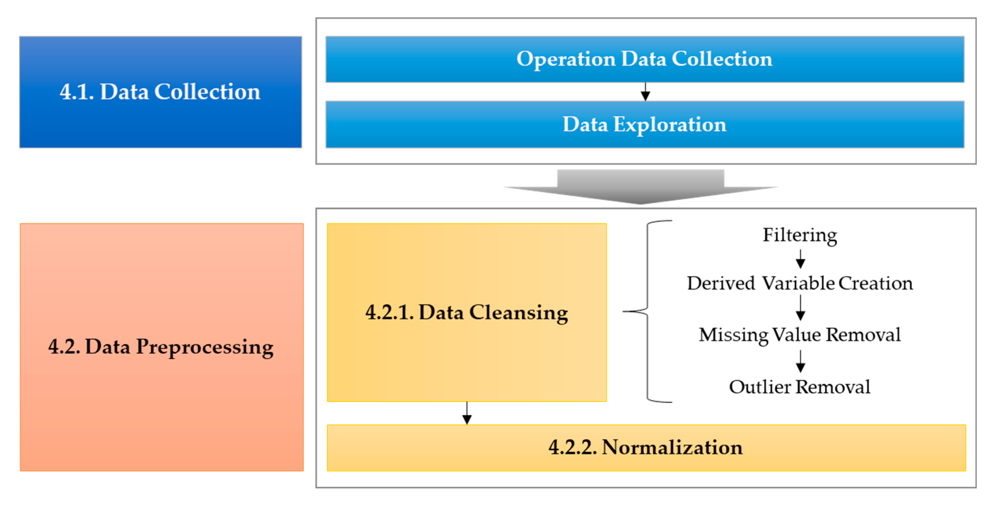
Data were collected for each stage of EAF operation, and the definitions and characteristics of each set of data were clarified. Next, the collected operation data were preprocessed to ensure better performance in the modeling process. The overall process of the data preprocessing can be confirmed in detail in Figure 5 below.

3.1. Data Collection

For this study, the EAF operation data of Company P’s STS-B steel plant were collected and stored in a high-performance data analysis server to develop a model. The data are information of 4598 heats from 19 February 2021 to 13 September 2021. They consist of a total of 53 variables, and each variable was measured, collected, and stored at each stage of operation. The description of each variable is detailed in Section 4.2.2. The computer’s DB uses Microsoft structured query language (MS-SQL), and the data analysis server uses python and pymssql libraries to extract operational data with SQL statements. The data collected for each operation stage were stored in four DB tables and extracted as individual files, and the heat number was merged into a key to form a single file and used. The data collected by the operation stage are as follows.

First, in the raw material charging stage, there are 32 variables related to the weight of the raw material and the production goal. Variables include the total weight of charged raw materials, weight by element (Si, C, Mn, P, S, Cr, Ni, Mo, Cu, FeCr), weight by origin (self-supply, import, domestic) of scrap, and weight by steel species (300 series, 400 series). There is a percentage of scrap in the total weight and a production target for steel type. Next, 12 variables exist in the melting stage. These variables include oxygen input, power input, power efficiency, water cooled panel (WCP) temperature, furnace bottom temperature, and waiting time before work. In the heating step, two variables of oxygen input and power input are stored, and tapping temperature is used as the Y feature in the tapping step.

In the charging stage into the AOD, which is the following process of EAF, six variables are stored, including EAF residual hot water, hot water, slag, chemical basicity, and hot water error rate. All six variables used in this step are information needed to predict the next Ch’ operation. The time of use differentiates the data that derive from the charging to tapping stages. In other words, performance information generated during the AOD charging of Ch’ produced just prior to the current operation is used to predict the tapping temperature of the Ch’ currently operating. It is, therefore, a simulation of the operating know-how of the operators. Because the information on the molten metal currently charged in the AOD indirectly reflects the condition of the electricity at the time the molten metal was discharged from the electric furnace, it can be an excellent indicator for the prediction of the following hot water temperature. Details of the feature types used at each stage of the operation can be found in

Table 2. Collected data from the database.

Stage	Attributes
	Weight	Volume	Power	Temperature	Time	Etc.
Charging (32 Variables)	Total weight, weight by element, weight by scrap type					Steel type, scrap ratio
Melting (12 Variables)		Oxygen injection amount	Power amount, power factor	WCP temp’, bottom temp’	Wait time
Refining (2 Variables)		Oxygen injection amount	Power amount
Tapping (1 Variable)				Tap temperature (Y Feature)
AOD charging (6 Variables)	(Previous Ch’) Remain weight, tap weight, slag weight			(Previous Ch’) Tap temperature		(Previous Ch’) Basicity, yield of tapping

below.

3.2. Data Preprocessing

Data preprocessing is a necessary process that affects model performance. This study secured data reliability through data cleansing and through the integration of variables with various scales through normalization [32]. It further secured data reliability through data cleansing, filtering through condition settings, the generation of derivatives reflecting operational knowledge, and the removal of missing values and outliers. After that, the cleaned data were normalized to ensure the model’s performance as much as possible. Data preprocessing used python programming languages and the basic libraries for data handling were NumPy and Pandas [33,34]. It was also conducted that the data analysis server should use the scikit-learn library for normalization [35].

3.2.1. Data Cleansing

Data cleansing aims to prevent the deterioration of a model that results from its training with unnecessary data by selecting only valuable data from that which has been collected [36].

The data used for this study were structured data extracted from the sensors in the EAF facility, though some missing values and outliers exist due to the data characteristics. Therefore, in this study, data cleansing processes such as filtering, missing value removal, and outlier removal were performed using a data distribution-based approach [37].

First, the collected data were filtered only in cases where steel type 304 was produced, and where the data were produced through two operations of raw material charging. The EAF process of the B steel plant produces various types of steel, such as STS 304, 316, 430, 321, and 410. However, steel types 316, 430, 321 and 410 do not have enough data to develop ML models. Therefore, only steel type 304, which occupies more than 70% of production, was selected. In addition, the number of raw materials charging per heat was generally doubled. However, when using scrap, which takes up more volume, the EAF roof cannot be closed. In this case, to maximize productivity, one more scrap charging action is executed and, thus, the operation must be carried out by charging the raw material three times. Unlike general operations where raw materials are input twice, in the case of atypical operations, such as the charging of raw materials three times, the charging data constitute approximately 7% of the collected data.

Due to the increase in the number of charging times, a relatively long operation time is required, which additionally causes a temperature drop. This was excluded from the dataset because of the characteristics of its development as a separate model from the case in which raw material is charged twice. After the data filtering, generation of the variables reflecting the domain knowledge of the operation was undertaken. The demand for electricity and oxygen is proportional to the mass of charged raw materials [38,39], so a derivative variable was generated to convert variables related to power and oxygen input that act as an energy source for EAF into energy per unit mass. The derivatives created were named ‘Power per weight’ and ‘Oxygen per weight’.

Next, missing values that might distort the model training process, significantly degrading performance or making smooth training impossible, were identified and removed. There is a possibility that a missing value may exist due to communication errors or sensor failures during the operation. In fact, as a result of checking the data, there were many cases where the data were omitted due to a failure of the tap temperature sensor.

Outlier means a very small or large value far outside the observed data range [40]. Traditionally, outliers have been removed by applying the interquartile range (IQR), a convenient method commonly used to detect outliers [41]. IQR refers to the difference between Q3, which means the top 75% point of the quartile, and Q1, which is the bottom 25% point and is expressed as Q3 − Q1. In applying the IQR, the parameter was performed by applying the most commonly used 1.5 IQR. The range from Q1 − 1.5 × IQR to Q3 + 1.5 × IQR was set as the normal range, and data with values outside this range were removed.

The initially collected data represented 4598 heats, but 45.1% of the data was removed while filtering, missing value removal, and outlier removal were performed, finally securing data representing 2523 heats. The step-by-step details of the data-cleaning task are described and the data loss rate can be comprehensively confirmed in

Table 3. Data loss during data cleansing.

Filter Condition		Number of Heats	Data Loss (%)
Raw Data		4598	-
Filtering	Steel type = 304	3230	29.8
	Number of charing = 2	3003	7.0
Missing Value Removal		2937	2.2
Outlierremoval	Tap temperature (before heat)	2795	4.8
	Power per weight	2666	4.6
	Water cooled panel (WCP) temperature	2654	0.5
	tap temperature (Y feature)	2523	4.9
Total data loss (%)		45.1

.

3.2.2. Data Normalization

Data normalization was conducted to maximize training performance. Data normalization is a process of unifying different scales between variables [42]. It has been proved through prior studies that the ML algorithm can secure better performance through normalization. Feature scaling using MinMaxScaler was confirmed to have relatively good performance in the regression model [43]. MinMaxScaler is a technique for converting data while assuming that the minimum value of each feature is 0.0 and the maximum value is 1.0 and is calculated by Equation (1).

$${x_i}^{\prime }=\frac{x_i-\min \left(x\right)}{\max \left(x\right)-\min \left(x\right)}$$

(1)

Table 4. Overview of data normalization.

Stage	Variable	Min	Max	Range	Stage	Variable	Min	Max	Range
First charge and melt	AvgTempBot	34	244	210	Second charge and melt	Oxygen_per_Weight	0.57	7.81	7.24
	AvgTempWCP	27	40	13		CConsCon	1.34	2.64	1.30
	MaxTempBot	55	280	225		CrConsCon	14.70	21.77	7.07
	MaxTempWCP	34	84	50		CuConsCon	0.11	0.32	0.21
	Power_per_Weight	149.49	260.50	111.01		FeCr_Conscon	0.00	0.55	0.55
	CConsCon	0.00	3.11	3.11		MnConsCon	0.31	1.10	0.79
	CrConsCon	0.00	25.83	25.83		MoConsCon	0.05	0.18	0.13
	CuConsCon	0.00	0.34	0.34		NiConsCon	4.21	8.05	3.84
	FeCr_Conscon	0.04	0.29	0.25		PConsCon	0.02	0.03	0.01
	MnConsCon	0.00	1.10	1.10		SConsCon	0.02	0.51	0.49
	MoConsCon	0.00	0.22	0.22		SiConsCon	0.68	1.78	1.10
	NiConsCon	0.00	9.88	9.88		SI300WGT	0	30,250	30,250
	PConsCon	0.00	0.03	0.03		SK300WGT	0	28,050	28,050
	SConsCon	0.00	0.83	0.83		SP300WGT	0	11,893	11,893
	SiConsCon	0.00	1.80	1.80		SP400WGT	0	2678	2678
	SI300WGT	0	29,960	29,960		SPGENWGT	0	7880	7880
	SK300WGT	0	27,740	27,740		Waittime	147	2964	2817
	SK400WGT	0	6390	6390	Refine	Oxygen_per_Weight	0.68	5.94	5.25
	SP300WGT	0	19,265	19,265		Power_per_Weight	34.92	93.03	58.11
	SP400WGT	0	6580	6800	Tapping	Tap_Temperature	1501	1633	132
	SPGENWGT	0	9560	9560
	Waittime	157	2501	2344	AOD charging (previous ch’)	Basicity	1.1	2.5	1.4
Second charge and melt	AvgTempBot	34	242	208		Remain_Weight	0	13,300	13,300
	AvgTempWCP	26	39	13		Slag Weight	0	19,300	19,300
	MaxTempBot	56	277	221		Tap_Weight Rate	76.6	145.2	68.6
	MaxTempWCP	33	88	55		Tap_Temperature	1432	1663	231
	Power_per_Weight	67.96	191.98	124.02		Tap_Weight	70,200	104,800	34,600

comprehensively presents each variable’s minimum, maximum, and range before MinMaxScaler.

Table 5. Meaning of each variable.

Variable	Definition
AvgTempBot	Average temperature (°C) measured with a thermometer installed on the floor of the EAF
AvgTempWCP	Average temperature (°C) measured in water cooled panel (installed on the EAF side)
Power_per_Weight	Electricity input per ton of scrap (kWh)
* ConsCon	* Ratio (%) of elements included in scrap (calculated by scrap sampling)
SI300WGT	300 series imported scrap weight (kg)
SK300WGT	300 series domestic scrap weight (kg)
SK400WGT	400 series domestic scrap weight (kg)
SP300WGT	300 Series Company P recycled scrap weight (kg)
SP400WGT	400 Series Company P recycled scrap weight (kg)
SPGENWGT	Other types of recycled scrap weight (kg) by P Company
Waittime	Waiting time before operation (sec)
Oxygen_per_Weight	Oxygen input per ton of scrap (Nm3)
Basicity	slag basicity
Remain_Weight	Remaining weight of hot water (kg)
Slag Weight	Amount of slag (kg)
Tap_Weight Rate	Tapping error rate = tapping amount/scrap weight (%)
Tap_Weight	Tap amount (kg)

* ConsCon: Constituent Condition.

explains the main variables and their definitions.

4. Tap Temperature Prediction Model (TTPM)

4.1. Modeling

Modeling includes the task of training an appropriate ML algorithm based on preprocessed data and selecting the optimal model by evaluating test data. This study applied six ML algorithms—linear regression, ridge, lasso, SVR-linear, polynomial, and radial basis function (RBF)—to predict the tapping temperature in real time during EAF operation. This study comprises one dependent variable, y, and two or more independent variables, making regression models appropriate. The authors selected the most basic linear regression model to compare performance with other models [44]. In addition, since there is a possibility of multicollinearity between variables, the ridge and lasso models were adopted [45]. Due to uncertainty as to whether the correlation between variables is linear or non-linear, sensor data affected by noise should be primarily be used, as a result SVR-linear, polynomial, and RBF were adopted [46].

Linear regression is a simple model that expresses a continuous dependent variable as a function of one or more independent variables [47,48]. Ridge is a model used to analyze multiple regression data with multicollinearity. Lasso is suitable for simple and sparse models with fewer variables because it processes linear regression through the selection of variables [47,48]. In other words, unlike ridge, lasso makes some coefficients (β) zero during the training process, so it can also play a role in the selection of key features to make the model more manageable and more concise to interpret [49]. SVR is an algorithm that applies an SVM to a regression problem. SVM is an algorithm that finds the optimal hyperplane for classifying two or more groups, and nonlinear properties can be given by introducing a kernel that maps data. It is with SVR that the regression equation was constructed by introducing a loss function into this SVM. SVR is characterized by high performance when removing or mitigating the effects of noise or outliers [50]. SVR could introduce a kernel as a mapping function to express nonlinear regression equations and general linear functions [51]. Typical nonlinear SVR algorithms include polynomial and radial basis functions.

For modeling, first, a preprocessed dataset was randomly sampled and separated into a training dataset and a test dataset at a ratio of 8:2. Second, the model was trained by exploring the optimal model parameters using k-fold cross-validation. In this study, k values were set to be 5, 10, and 20. Third, the performance of the training model was derived by applying the test data, and the optimal model was selected. Python’s scikit-learn and gridsearchcv libraries were used for modeling and model parameter optimization on the data analysis server. In addition, for data visualization, mat-plotlib and seaborn libraries were used. Figure 6 illustrates the overall flow of modeling.

4.2. Model Training with Parameter Optimization

4.2.1. Parameter Optimization

Model parameter optimization using k-fold cross-validation was performed to overcome the statistical dependence problem between the training and test datasets and prevent overfitting [52,53]. Though there is no theoretically established procedure for calculating the optimal value of k [51], in this study, the authors set k = 5, k = 10, and k = 20 to train and optimize the parameters. In the case of k = 5, the MAE value is 0.120789 for ridge, 0.120765 for lasso, 0.122903 for SVR linear, 0.120078 for SVR polynomial, and 0.119452 for SVR RBF. The MAE values for each model with k = 10 are 0.120892 for ridge, 0.120812 for lasso, and 0.123187 for SVR linear. The SVR polynomial is 0.120125, and the SVR RBF is 0.119812. The MAE values for each of the five models for k = 20 are 0.121354, 0.121265, 0.123843, 0.120228, and 0.120013, respectively. The training results for the five algorithms showed an optimal performance at k = 5.

Table 6. Parameter optimization results for various values of k.

k-Fold	Ridge	Lasso	SVR Linear	SVR Polynomial	SVR RBF
k = 5	0.120789	0.120765	0.122903	0.120078	0.119452
k = 10	0.120892	0.120812	0.123187	0.120125	0.119812
k = 20	0.121354	0.121265	0.123843	0.120228	0.120013

presents the results of parameter optimization for k = 5, k = 10, and k = 20. Throughout this paper, the results of parameter optimization in the case of k = 5 are shown graphically.

The k-fold cross-validation proceeded as follows. First, the entire dataset was divided into training datasets and test datasets. In this study, the dataset was divided at a ratio of 8:2. Next, the training dataset was separated into k folds to be used for training and validation purposes. After that, the first fold was set as a validation dataset and the remaining folds as a training dataset. After the model training, the mean absolute error (MAE) was applied as the first validation. Denormalization was not conducted since the purpose of the MAE calculated here is to make a relative comparison between models. After that, the same process using the next fold as a validation dataset was repeated k times. The average of k MAEs calculated after repeated progress is taken and determined by the model’s performance. It is k-fold cross-validation that repeats this entire process while changing the parameters of the ML algorithm and finding the parameters in which the MAE records the lowest value. The parameter optimization operation of each model was performed using the k-fold cross-validation described above. The linear regression (LR) algorithm is a simple algorithm that learns to minimize errors within the training dataset and does not have any separate parameters. Therefore, the parameters were optimized for the model to which the remaining five algorithms were applied.

Figure 7a below displays the results of parameter optimization for the model to which the ridge algorithm was applied. The Y-axis represents the MAE, and the X-axis is the algorithm parameter α. Ridge calculates the error through Equation (2), which reduces the complexity of the model and prevents overfitting by adding the square of each coefficient (β) to the error to reduce the coefficient [54]. This method is L2 regularization. As a result of parameter optimization, α = 0.25 showed the minimum value. Figure 7b shows the parameter optimization result for the lasso algorithm model. Likewise, the Y-axis represents the MAE, and the X-axis is the algorithm parameter α. Lasso calculates the error through Equation (3), and the difference from ridge is that it reduces the coefficient by adding the absolute value of each coefficient (β) to the error. Unlike ridge, lasso prevents overfitting through L1 regularization [40]. The parameter optimization result confirmed that the MAE showed the minimum value at α = 3 × 10⁻⁵.

$${Error}_{ridge}=\frac{1}{M}{\sum }_{i=1}^M{\left(y_i-{\widehat{y}}_i\right)}^2+\alpha {\sum }_{j=0}^n{{\beta }_j}^2$$

(2)

$${Error}_{lasso}=\frac{1}{M}{\sum }_{i=1}^M{\left(y_i-{\widehat{y}}_i\right)}^2+\alpha {\sum }_{j=0}^n\left|{\beta }_j\right|$$

(3)

Equation (4) and Figure 8 present the ε intensive loss function, which is a loss function widely used in SVR algorithms. The ε intensive loss function forms a vertical section in the range of 2ε (−ε, ε) of the predicted value. The error is ignored if there is an actual value within the interval, although it differs from the predicted value. C represents the cost parameter of the SVR model. If there is an actual value outside the interval, the error is calculated by the multiplier of C. Through this process, SVR assumes that noise is included in the data and therefore does not aim to predict the actual value, including noise, perfectly. In other words, by allowing the difference between the actual value and the predicted value within the appropriate range (2ε), the model’s performance can be improved [55].

$${Error}_{SVR}=\frac{1}{2}{\sum }_{j=0}^n{{\beta }_j}^2+C{\sum }_{i=1}^M\left({\xi }_i+{\xi }_i^{\mathrm{*}}\right)$$

(4)

$$s.t\left(\widehat{y_i}-y_i\right)\le \epsilon +{\xi }_i, \left(\widehat{y_i}-y_i\right)\le \epsilon +{\xi }_i^{\mathrm{*}},{\xi }_i\ge 0, {\xi }_i\ge 0,{\xi }_i^{\mathrm{*}}\ge 0$$

Figure 9 is the result of parameter optimization for the model to which the SVR linear algorithm is applied. As a result of parameter optimization, it was confirmed that the MAE showed the minimum value at C = 0.3.

SVR polynomial and RBF are algorithms that use a nonlinear kernel, and, unlike linear, the user must additionally set the gamma parameter. This parameter sets the distance at which one data sample exerts an influence, with the larger the gamma, the smaller the influence exerted by the data sample. In other words, the curvature of the crystal boundary can become complicated or simple depending on the gamma. Like C, if it is too large, there is a risk of overfitting, and if it is too small, under-fitting may occur. Therefore, the user has to empirically find the optimal parameter by applying various ranges of values, not only for C but also for gamma. In this study, the gridsearchcv library of python was used.

Figure 10a is a diagram expressing the result of the parameter optimization for the SVR polynomial model as a heatmap. The parameters C and gamma of the model are set to Y-axis and X-axis, respectively and MAE (score), calculated by applying k-fold cross-validation in the corresponding parameter, is recorded. As a result of parameter optimization, the MAE was the minimum at C = 0.5 and gamma = 0.1 (degree = 3, ε = 0.01). Similarly, Figure 10b is the result of parameter optimization for the model to which the SVR RBF algorithm was applied. The parameter optimization resulted in an MAE showing a minimum value at C = 5.0 and gamma = 0.05 (degree = 3, ε = 0.01).

The result of model parameter optimization is as follows. Ridge, lasso, and SVR linear which are linear models, have α = 0.25, 3 × 10⁻⁵, and C = 0.3 respectively. SVR polynomial, a nonlinear model, showed C = 0.5 and gamma = 0.1, while SVR RBF showed C = 5.0 and gamma = 0.05.

4.2.2. Model Training

To confirm that the model training was correctly performed, each model’s prediction results using six ML algorithms were synthesized to calculate error functions such as root mean square error (RMSE), MAE, and R². The training data used 2019 heats randomly sampled among 80% of the 2523 heats for which preprocessing was completed.

As a result, the model using the SVR RBF algorithm was derived with the best training performance with RMSE 18.99, MAE 14.46, and R² 0.334. There was no significant performance difference between linear regression, ridge, and lasso. In addition, the models using the SVR presented excellent performance as a whole, with the polynomial and the RBF using a nonlinear kernel performing relatively excellently. The performance of the nonlinear model was derived better than the linear model’s performance. In model training, the higher the complexity of the model, the more likely it is to exhibit superior performance.

Table 7. The performance result of model training with parameter optimization.

Error Functions	Linear	Ridge	Lasso	SVR
				Linear	Polynomial	RBF
RMSE	19.55	19.57	19.57	19.74	19.16	18.99
MAE	15.37	15.41	15.41	15.27	14.68	14.46
R2	0.294	0.292	0.293	0.280	0.322	0.334

lists the model training results obtained by parallel parameter optimization.

4.3. Implementation and Validation of TTPM

4.3.1. Measurement

To verify the training model, an off-site and on-site test were implemented twice. The off-site test involves selecting TTPM by testing six models and performance evaluation. The on-site test applies TTPM to the actual production site to evaluate technical and financial performance, and it will be explained in detail later in Section 6. First, the off-site test aimed to select TTPM through performance comparison between training models. Therefore, the model performance was confirmed by three error functions such as MAE, RMSE, and R², using the test dataset. The smaller the MAE and RMSE values, the better the performance. In particular, since RMSE is a factor that can directly measure the performance when the model is applied to the actual site by comparing it with the standard deviation of the tapping temperature, TTPM was selected after checking the RMSE. In the on-site test, the best model for the off-site test was selected as TTPM, applied to the production site, and the evaluation was performed by checking the accumulated operation data. This process aimed to compare the performance of the newly developed TTPM with the operating capability of operators. Therefore, the quantitative effect of reducing the tap temperature deviation of TTPM was confirmed by calculating the standard deviation and MAE of the tapping temperature by classifying whether or not the AI automatic operation function was applied. The detailed formulas used in the performance evaluation are shown in

Table 8. Performance measurement metrics.

Section	Metric	Formula
Tap temperature prediction model (TTPM)	MAE	$\frac{1}{\mathrm{n}}{\displaystyle \sum _{\mathrm{i}=1}^{\mathrm{n}}}\left|{\widehat{y}}_i-y_i\right|$
	RMSE	$\sqrt{\frac{1}{n}{\displaystyle \sum _{i=1}^n}{\left({\widehat{y}}_i-y_i\right)}^2}$
	R2	$\frac{SST}{SSE}=\frac{{\sum }_{i=1}^n{\left({\widehat{y}}_i-\stackrel{-}{y}\right)}^2}{{\sum }_{i=1}^n{\left(y_i-{\widehat{y}}_i\right)}^2}$
System development and application on production site	SD	$\sqrt{\frac{{\sum }_{i=1}^n{\left(\stackrel{-}{y}-y_i\right)}^2}{n}}$

below.

4.3.2. Performance Evaluation and Validation

The performances of six ML models were evaluated using a test dataset randomly sampled at 20% from the entire dataset (504 heats). Among the six models, the SVR-RBF model had the best performance with RMSE 20.14, MAE 16.05, and R² 0.308. Significant differences between the linear regression, ridge, and lasso models were not found. Overall, it was confirmed that the performance of SVR polynomial and SVR RBF using nonlinear kernels was relatively superior to other models. In addition, the SVR linear model presented low performance compared with the linear model. EAF operation is a process in which various variables are combined. A model using a nonlinear algorithm shows a better performance than a model using a linear algorithm.

Table 9. The performance results of the model test.

Error Functions	Linear	Ridge	Lasso	SVR
				Linear	Polynomial	RBF
RMSE	20.57	20.62	20.59	20.73	20.35	20.14
MAE	16.51	16.62	16.60	16.66	16.27	16.05
R2	0.278	0.275	0.277	0.267	0.293	0.308

shows the detailed performance results of the six models.

The SVR algorithm uses a loss function and ignores the error if the difference between the actual and predicted values exists within a certain range. It is assumed that the data contain noise, so users cannot aim to predict the actual value, including noise, perfectly. Due to the characteristics of the algorithm, the SVR can play a role in mitigating the noise contained in the data [50]. EAF has an inferior field environment, one which includes temperature and dust, so some noise around the sensors is inevitable. Weight and temperature are representative physical quantities that cause noise depending on the surrounding environment and the sensor’s lifespan. It is to be expected that relatively excellent performance is achieved as the algorithm’s mechanism complements this part.

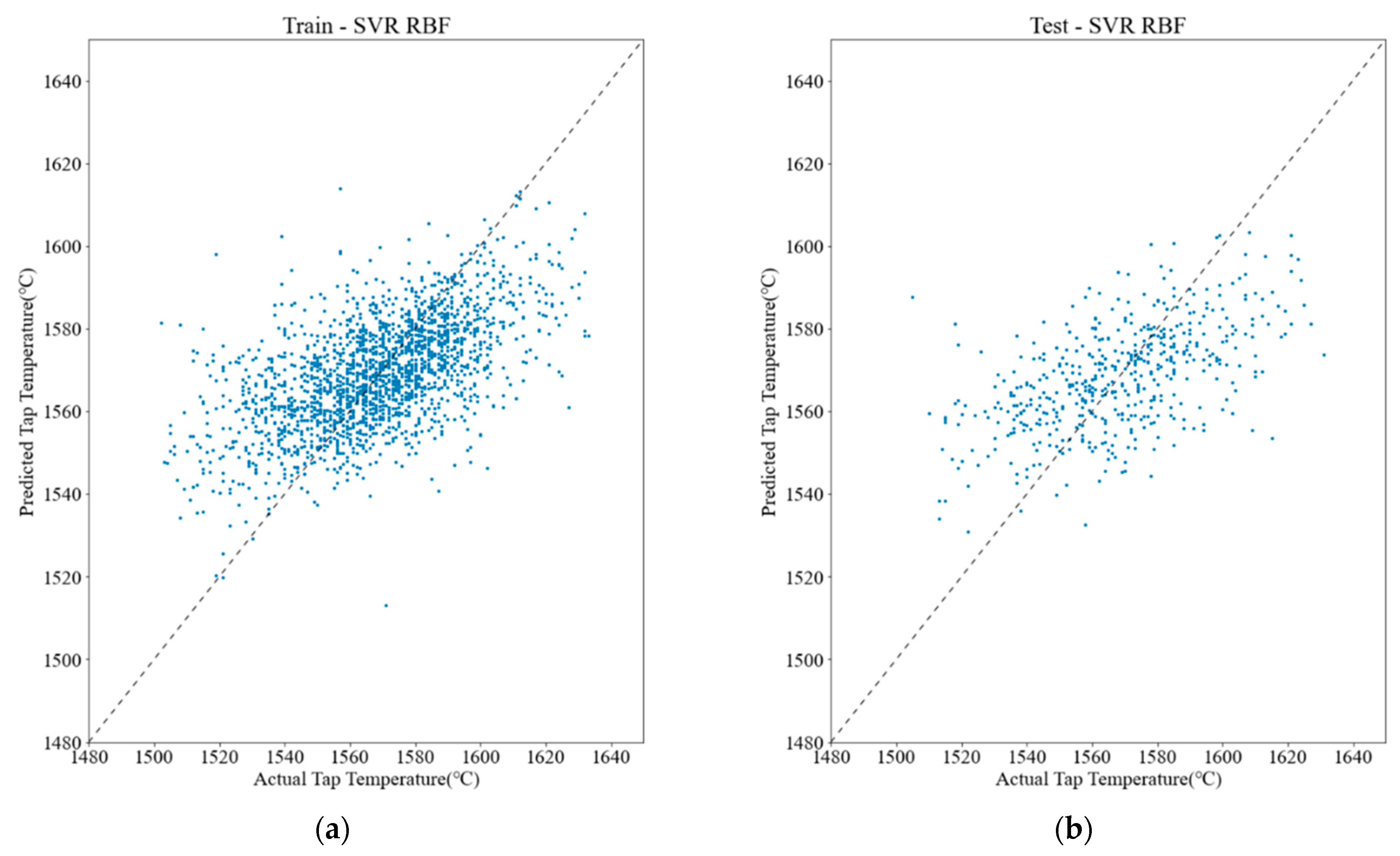
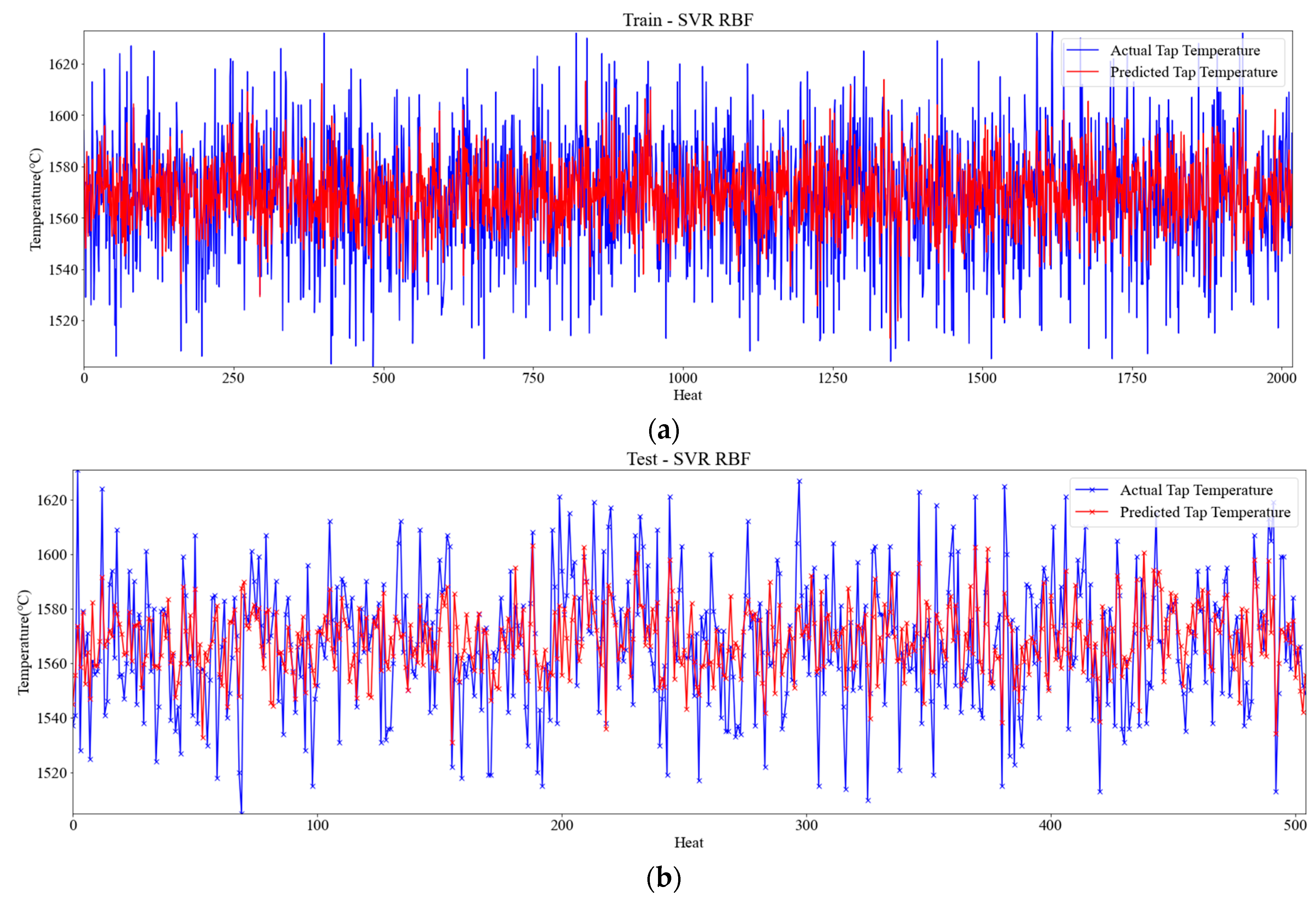
The operator proceeds with the operation by predicting and setting the amount of electricity that can reach 1580 °C of tapping temperature based on subjective standards. Therefore, the performance can be confirmed by directly comparing the standard deviation of the actual tap temperature measured as an operational result and the RMSE of the tap temperature predicted by the developed model. As a result of the analysis of the operational data in which the operator manually set the amount of electricity, the standard deviation of the tap temperature was 31.4. However, the model’s performance applying the SVR RBF algorithm was measured at 20.14 for the predicted tap temperature RMSE. This is analyzed because it is an improvement of more than 30% compared with manual operating. It is expected that the deviation of the tapping temperature will be able to be reduced by more than 30% compared with manual operating when the developed model is applied to the site. In the test results, the SVR RBF model, which showed the best performance in MAE and R² as well as RMSE, was selected as the best model. A site application test was implemented. Figure 11 is a graph drawn of the tap temperature performance and the prediction of the SVR RBF model. Figure 11a represents the training dataset, and Figure 11b the test dataset.

Figure 12a demonstrates the training results of the model applying the SVR RBF, and Figure 12b shows the test results for predicting the tap temperature of the SVR RBF model. In Figure 12b, the gap between actual and predicted values varies. The actual temperature is the temperature of molten stainless steel measured after the operation’s end (Y), and the expected temperature is the value predicted by the model (Y’) with the corresponding data. Even if there is a significant difference between the predicted and actual values, this difference can be meaningful. For example, suppose the actual temperature is 1520 °C, and the predicted temperature is 1565 °C. When this model is applied to the field, the power input would be stopped later than if the operator had stopped the power supply. Additional power input is therefore required. In this case, the actual temperature is predicted to be approximately 1520 + (1580 − 1565) = 1535 °C. This shows better performance compared with the operator’s judgment. However, when predicted at 1475 °C with the same temperature deviation of 45 °C, the actual temperature shows a rather large error of 1520 + (1580 − 1475) = 1625 °C. Therefore, if the model can predict the tap temperature between 1580 °C and the actual temperature, it is considered to show better performance than the operator’s judgment.

5. System Application and Performance on the Production Site

5.1. The Concept of System Application

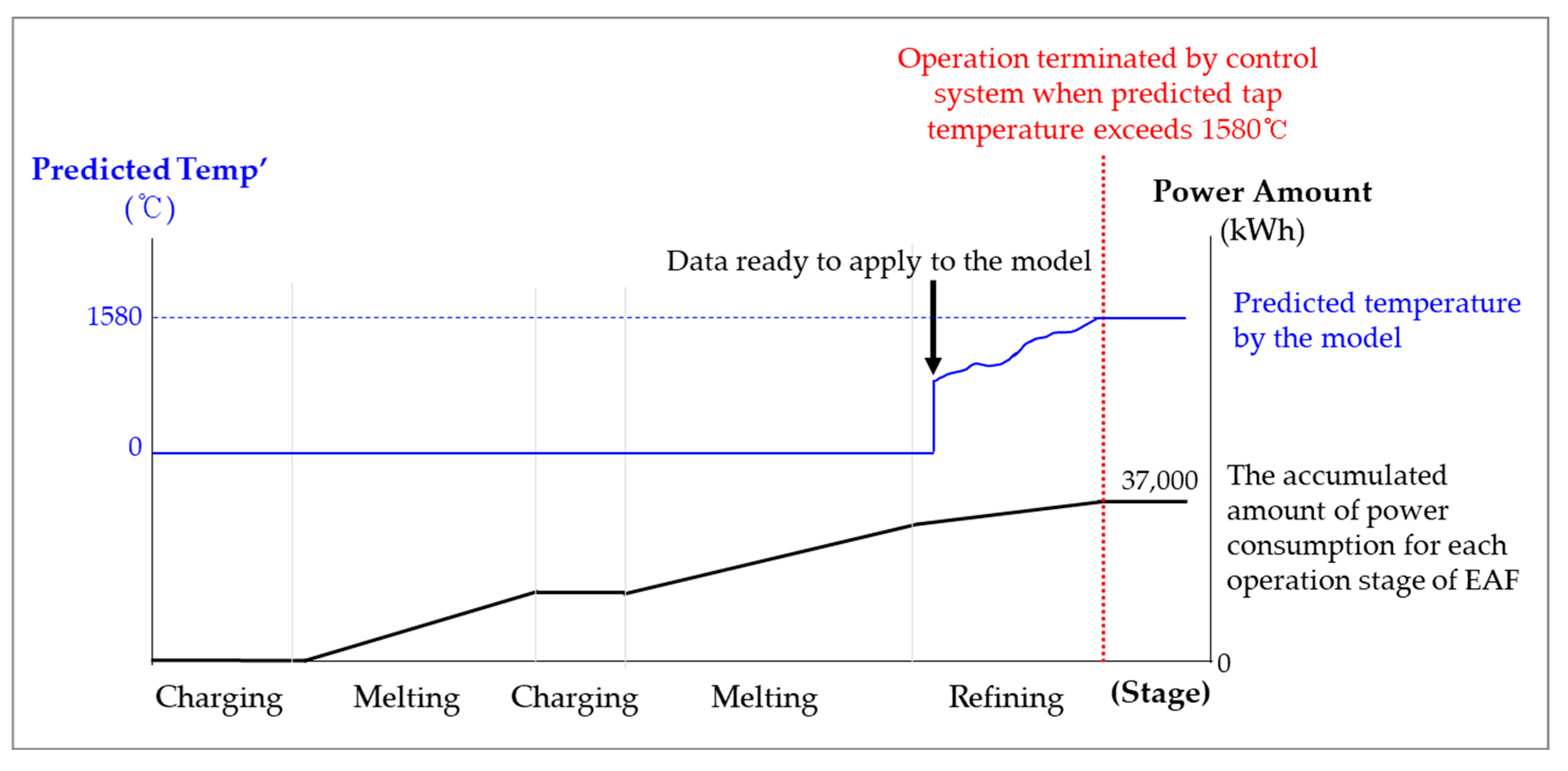
In order to verify the effectiveness of the TTPM developed using the operational data of Company P’s STS B steel mill EAF, an on-site test was applied. This process is organized into four shifts, and production is carried out during two shifts each day. It is therefore operated 24 h a day, except in cases of equipment failure or planned maintenance work. When TTPM is applied to the site, an AI automatic operation function that automatically controls production according to the tap temperature predicted by TTPM is developed. Its goal is to minimize factors that decrease productivity and that may be caused by changes in operating conditions and to remove factors that increase the operator’s workload. To this end, hardware installation, communication between devices, and software were developed and applied to the site. The developed TTPM operates as follows for each production stage. The predicted value is 0 in the first charging and melting stage and the second charging and melting stage because the data for predicting the tapping temperature is not prepared. The tap temperature is predicted from the heating stage, where all features for prediction are prepared. The predicted tapping temperature increases as power and oxygen are continuously input. When using the AI automatic operation function, if the predicted tapping temperature exceeds 1580 degrees or the power-on operation is interrupted manually, the predicted tapping temperature value stops changing. A detailed timing chart for each operation stage is shown in Figure 13.

In connection with the TTPM’s timing chart described above, the AI automatic operation function is applied to the production through the following process. The operator first decides whether or not to use the AI automatic operation function. If the operator decides to use the AI automatic operation function, they will click the button on the HMI to turn on the function. The button then turns red and tells the operator that the function is working. If the AI automatic operation function is not used, the operation proceeds based on the power input amount set by the operator as before. When the operation enters the heating stage and all the data needed for prediction are ready, the model begins to output the predicted values. If there is a missing value or an outlier in the X factor, or if the steel type is different from type 304, the tapping temperature cannot predict. Therefore, if the AI automatic operation is turned on, it is ignored, and the operator proceeds with the existing manual operation. As power and oxygen are supplied, the predicted tap temperature rises, and the power-on operation is automatically terminated when the target tap temperature exceeds 1580 °C. After training, four groups of operators with more than 20 years of experience tested the AI automatic function on the site for five months from 1 October 2022. Figure 14 presents the process of AI automatic operation function operation.

5.2. Hardware Setup

The following hardware installation and software development work preceded on-site application tests. A new model server for the execution of a model was installed in a data center with PCs that store various operational data. In addition, the communication interface was carried out between the model server, the PC, and the programmable logic controller (PLC) installed on the site. As for the communication interface, SQL commands were developed to access the DB of the PC in the model server and extract the operating data stored in each stage. The command was written using the pymssql library of python.

Next, data that should be reflected in the TTPM in real time, such as power and oxygen input, were transmitted from the PLC to the model server. Then the logic was developed to receive the tap temperature predicted in the model. On the PLC side, the manufacturer’s own programming tool, simatic manager, was used to create transmission control protocol/internet protocol (TCP/IP) transmission and reception programs. Additionally, communication programs were developed using python’s socket library on the model server.

Whether the developed model correctly predicted the tap temperature was confirmed as follows. First, the developed model was transplanted to the model server, and the model was executed with operational data received through communication. The model developed in the data analysis server was ported to the model server in the form of a ‘.pkl’ file through the pickle library of python. Prior to the completion of the secondary melting step, no necessary operational data were prepared, so exceptions had to be made. Additionally, outliers or missing values were excluded. Furthermore, a function to save the predicted tapping temperature and the actual values of the features used for prediction in log form was developed using python in order to facilitate analysis of future test results.

A new user interface (UI) was developed on the HMI to interface with the operator in providing information predicted by the model to the operator and so that they may receive input on whether to use the AI automatic operation function. The information provided to the HMI is the tapping temperature predicted by the model and the amount of power input required to reach 1580 °C. The power input was calculated using Equation (5) to estimate the approximate end of the operation. The specific heat was calculated using the average value of 0.26, which was determined by applying the training data.

(1580—predicted tap temperature) (°C) × total weight (ton) × average of specific heat (kW/ton∙°C)

(5)

A command button was created that allows the operator to input whether or not to use the AI automatic operation function with a mouse. As a result, the function can be turned on and off at any time during operation. Unexpected situations can occur at any time during production work, and it is necessary to maintain productivity according to the operational situation of the subsequent process, rather than according to any one single process, so the AI automatic function was designed to respect the operator’s decision as much as possible. The PLC’s existing operation control program was modified to automatically terminate the operation according to the predicted tap temperature when the corresponding button was turned on.

The overall system configuration and data flow reflecting the hardware installation, communication establishment, and system improvement work described above are as follows. First, a data analysis server for model development is installed in the office, and the operation data for analysis is extracted from the operation DB of the PC. After completion of TTPM development through model training and testing, it is implanted into the model server. The model server is a server that runs TTPM and was newly installed in the data center for this study. The model server periodically extracts Ch’s data currently in operation from the PC’s operation DB. It receives the changing electricity and oxygen input amount in real time from the PLC that controls the overall process. After merging the received data, the TTPM predicts the tap temperature and sends it to the PLC along with the calculated power input using the average specific heat. The HMI searches the data of the PLC and provides the predicted tap temperature and power input information to the operator. The operator turns the AI automatic operation function on or off through the HMI, and the PLC controls the endpoint of the operation by reflecting this. The hierarchy and data flow of the whole system are detailed in Figure 15.

The training and testing of TTPM used the Windows 10 operating system and python 3.8.1. The model server was developed using python in the Linux operating system. The PLC for process control installed on site is a Siemens’ S7 400 model. The communication program development and EAF control program improvement were carried out using the simatic manager program to open communication and implement AI automatic operation function. The detailed specifications and uses of the facilities constituting the system are shown in

Table 10. System specification and usage.

PLC	Model Server	Data Analyzer Server	Software
Siemens S7 416-2 CPU Work memory 8 MB 1st interface MPI/DP 2nd interface PROFIBUS DP	CPU: Intel Core i7 3.0 GHz RAM: 8 GB HDD: 1TB + 4 TB OS: Linux (Redhat)	CPU: Intel Core i7 3.2 GHz RAM: 16 GB HDD: 1 TB GPU: GeForce GTX 1070 OS: Windows 10	Language: Python 3.8.1 Libraries: pandas 1.3.4, matplotlib 3.4.3, numpy 1.20.3, scikit-learn 0.24.2, seaborn 0.11.2 Jupyter Lab 3.2.1 Jupyter Notebook 6.5.1
process control	model execution (new installation)	model development

.

5.3. System Performance on Site

This section describes the on-site application test results of TTPM. The on-site application test results were conducted for five months from 1 October 2021 to 28 February 2022. Quantitative analysis was conducted by matching the operation data stored in the PC with the log data stored in the model server.

First, the test results in terms of performance using the error function are as follows. Since both manual operation and AI automatic operation were the results of operating at a target tapping temperature of 1580 °C, the MAE was calculated based on this when calculating the error function. In other words, the average was calculated by setting the amount that the actual tap temperature exceeded or fell below 1580 °C as an error. A total of 2599 Ch’ was produced during that period. Among these, a total of 1388 Ch’ were produced in predictable cases, excluding cases that were not of steel type 304, outliers, or unpredictable missing values. Of the 1388 Ch’, 613 Ch’ used the AI automatic operation function, and the remaining 775 Ch’ operated manually, recording a prediction model application rate of 44.2%. Looking at the error function, first, MAE presented a total of 19.9, while the manual operation was 21.1, and AI automatic operation recorded 18.4, an improvement of 13%. The standard deviation was 25.9 overall, and the manual operation recorded 27.9, but the AI automatic operation recorded 23.1, an improvement of 17%. The average tap temperature was 1575.2 °C for AI automatic operation, 0.7 °C lower than 1575.9 °C for manual operation, and there was no significant difference. In conclusion, the molten metal temperature tapped after automatic operation using the tap temperature that was predicted based on the operation data was relatively superior in both deviation and standard deviation compared with the target temperature derived from the manual operation based on subjective judgment. Detailed data can be found in

Table 11. The performance result of on-site implementation.

Metrics	Total	Operation Types
		Manual	AI
Heats (Ch’)	1388	775	613
Average Tap Temperature	1575.6	1575.9	1575.2
MAE	19.9	21.1	18.4 (△13%)
SD (σ)	25.9	27.9	23.1 (△17%)

.

There are many operating ratios in manual operation with a significant temperature deviation, with the tapping temperature measured above 1610 °C or below 1530 °C. In the AI automatic operation, as the hot water temperature standard deviation was improved by 17% and the MAE by 13%, the frequency of such cases was drastically reduced.

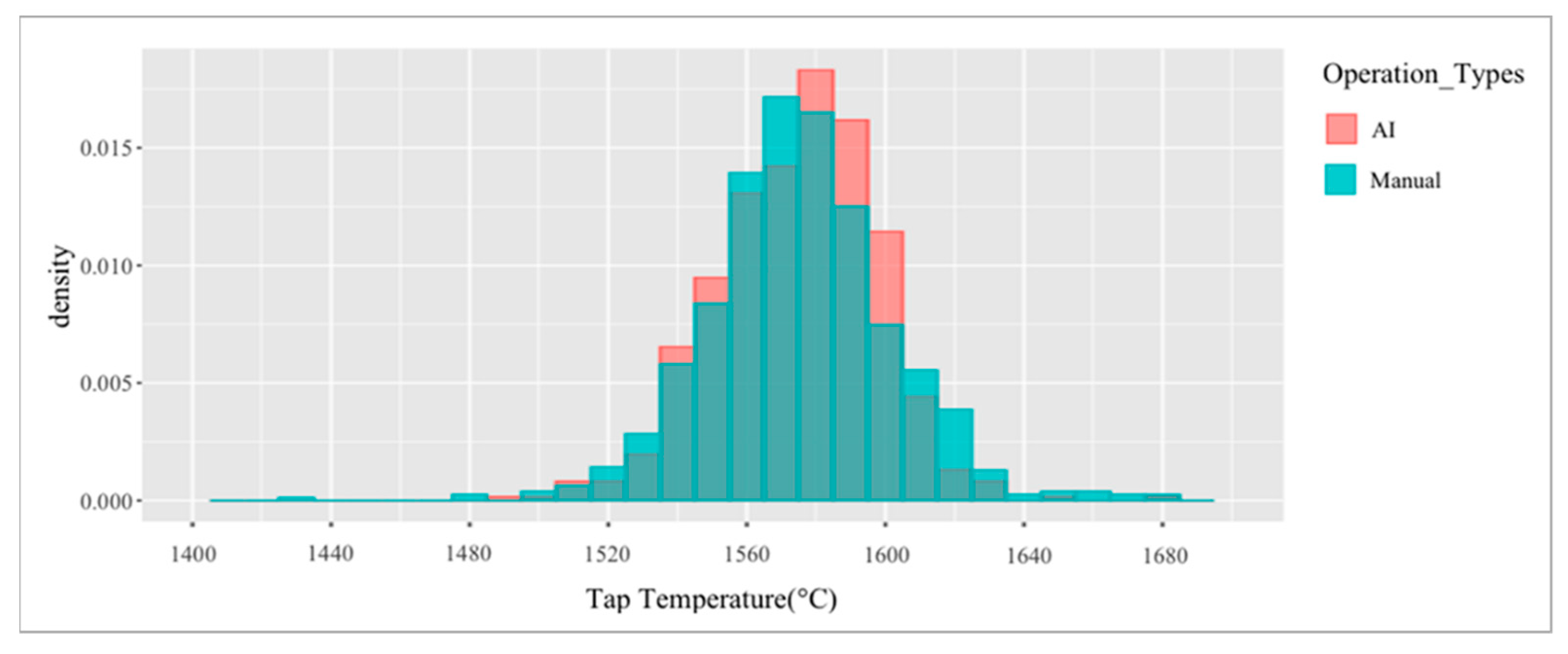
TTPM based on the SVR RBF algorithm used in the on-site test recorded MAE 16.05 and RMSE 20.14, but the result applied to the actual operation derived an error function 10% to 15% lower than this. This seems to be because the model trained using the February to September 2021 operation data was applied for five months from October 2021, so process variables that changed over time were not reflected. However, this problem is expected to be mitigated if periodic model retraining is performed using the latest data that reflect changing facility conditions over time. Figure 16 shows the distribution of tapping temperature in units of 10 °C by dividing AI automatic operation and manual operation, and the effect of reducing the tap temperature deviation can be visually confirmed.

5.4. Economic Effects and Economic Analysis

This section calculates the economic effect of the on-site application of TTPM. First, the system was improved so that the power input amount through the HMI was stored in operation DB to calculate the quantitative effect. For 49 days after system improvement (from 11 January 2022 to 28 February 2022), 153 Ch’ using the AI automatic operation function were analyzed among 638 Ch’ operation data. Quantitative effects were calculated for the improvement of AI automatic operation compared with manual operation.

The economic effect was calculated from electricity cost and fixed cost reduction. First, by conducting AI automatic operation compared with the amount of power input set by the operator during the period, it was possible to save 282 kWh/Ch’, a total of 43,250 kWh of electricity. Converting this to an annual basis is expected to reduce power input by 328,880 kWh/year. When applying 0.065 USD/kWh, the power unit, as of 2021, is expected to save electricity costs by 21,013 USD/year. Suppose electricity is not generated by renewable energy resources (e.g., thermal power, etc.), in that case, this saving in power consumption brings environmental benefits in the long term by reducing carbon emissions per unit of production. In the context of global efforts to reduce energy consumption and carbon emissions in all industries, it is expected that this study can contribute to carbon reduction.

The average tapping temperature of 638 Ch’ operated during the corresponding period was 1577.1 °C and the average tapping temperature of 153 Ch’ operated by AI automatic operation was 1577.5 °C. It was determined that it is possible to save the amount of power input by reducing the deviation while maintaining the average tapping temperature. Second, as the operating time was shortened due to the reduction in power input, we calculated fixed costs that could be saved through additional production. According to the 328,880 kWh/year mentioned above saving in power input, 482.4 min of additional operation may be possible, which is the time to produce a further 7.4 Ch’. Accordingly, the fixed cost of 66,663 USD/year is expected to be saved through an increase in production of 654.9 tons. This reduction effect was calculated using the 2021 performance-based T-T, fixed cost, speed of power input, and average output operation index. Detailed figures are confidentially related to the company’s manufacturing cost, so they are not described in this paper. In addition, as a qualitative effect, the operator’s workload can be reduced by automating the power input setting task. It is also expected that the operation efficiency of an unskilled operator can be increased.

Next, the authors analyzed the economic feasibility of this study. The economic analysis assesses how much future cash flows expected from investment might contribute to a company’s goal as it exceeds or falls short of the current investment [56]. This essentially involves an assessment of costs and benefits. The assessment method is divided into the non-discounted cash flow (non-DCF) and discounted cash flow (DCF) methods. Non-DCF includes the payback period (PP) in Equation (6) and the average rate of return (ARR) in Equations (7) and (8), which do not take into account the time value of money by omitting the discount procedure for calculating the present value of cash inflows or outflows.

$$\mathrm{P}\mathrm{a}\mathrm{y}\mathrm{b}\mathrm{a}\mathrm{c}\mathrm{k}\mathrm{P}\mathrm{e}\mathrm{r}\mathrm{i}\mathrm{o}\mathrm{d}\left(\mathrm{P}\mathrm{P}\right)=\frac{CostofInvestmet}{AnnualCashInflows}$$

(6)

$$\mathrm{A}\mathrm{v}\mathrm{e}\mathrm{r}\mathrm{a}\mathrm{g}\mathrm{e}\mathrm{R}\mathrm{a}\mathrm{t}\mathrm{e}\mathrm{o}\mathrm{f}\mathrm{R}\mathrm{e}\mathrm{t}\mathrm{u}\mathrm{r}\mathrm{n}\left(\mathrm{A}\mathrm{R}\mathrm{R}\right)=\frac{AverageAccountingProfit}{AverageInvestment}\times 100$$

(7)

$$\mathrm{A}\mathrm{v}\mathrm{e}\mathrm{r}\mathrm{a}\mathrm{g}\mathrm{e}\mathrm{I}\mathrm{n}\mathrm{v}\mathrm{e}\mathrm{s}\mathrm{t}\mathrm{m}\mathrm{e}\mathrm{n}\mathrm{t}=\frac{InitialInvestmet+SalvageValue}{2}$$

(8)

DCF techniques include the net present value (NPV) calculated in Equation (9), and internal rate of return (IRR) in Equation (10). These are methods of considering the time value of money by converting the capital cost of an investment into a present value through a discount.

$$\mathrm{N}\mathrm{e}\mathrm{t}\mathrm{P}\mathrm{r}\mathrm{e}\mathrm{s}\mathrm{e}\mathrm{n}\mathrm{t}\mathrm{V}\mathrm{a}\mathrm{l}\mathrm{u}\mathrm{e}\left(\mathrm{N}\mathrm{P}\mathrm{V}\right)=\sum _{t=1}^t\frac{C_t}{{\left(1+r\right)}^t}-C_0$$

(9)

where

t: Time of the cash flow;

C₀: Initial investment;

C_t: Net cash flow;

r: Discount rate.

$$\mathrm{I}\mathrm{n}\mathrm{t}\mathrm{e}\mathrm{r}\mathrm{n}\mathrm{a}\mathrm{l}\mathrm{R}\mathrm{a}\mathrm{t}\mathrm{e}\mathrm{o}\mathrm{f}\mathrm{R}\mathrm{e}\mathrm{t}\mathrm{u}\mathrm{r}\mathrm{n}\left(\mathrm{I}\mathrm{R}\mathrm{R}\right):\mathrm{N}\mathrm{P}\mathrm{V}=0=\sum _{t=1}^t\frac{C_t}{{\left(1+r\right)}^t}-C_0$$

(10)

PP calculates how many years it takes to retrieve investment costs, and the shorter the payback period, the more liquidity the company can secure. However, there is a disadvantage: the benefits incurred after the recovery period are not considered [57]. ARR divides the annual average profit expected from the investment by the average annual investment and calculates the return based on the accounting–calculated profit. It has the advantage that the calculation method is simple because it uses book profits, but it has the disadvantage that it is not a cash flow-based method [58]. NPV applies a discount rate to all cash flows arising from an investment, refers to the amount that limits the initial investment costs, and determines that it is economical if it is greater than zero. It has the advantage of considering cash flow, not accounting profit, and assuming that the cost of capital is reinvested at the internal rate of return during the investment period. A disadvantage is that it is difficult to estimate the cost of capital accurately. NPV is the most widely used economic evaluation method for overcoming PP’s limitations [59]. IRR is an indicator used to measure the profitability of an investment project, and refers to the discount rate at which cash flows throughout the project are converted into present values so that the sum is equal to investment expenditure. The higher the domestic return, the greater the project’s profitability and the domestic return determines the minimum return to make the project viable.

Based on the economic effects mentioned above, the IRR was found to be 35.8% due to setting the standard for 15 years of equipment service life, 6.6% discount rate, 3% maintenance cost, 27.5% corporate tax, and one year of business period. This figure exceeds 8% of the hurdle rate managed internally by Company P, and the economic effect is considered sufficient. Suppose performance is not maintained through continuous training of the predictive model, in that case, a lower effect may be calculated than the expected effect, but the corresponding issue shall be excluded from this paper.

5.5. Lessons Learned from the On-Site Test

The on-site application test is a task that cannot be performed without the operator’s cooperation because the operator must approve whether or not the AI model is applied. Therefore, the most challenging part of the on-site tests was persuading operators to familiarize themselves with the existing operation method. About 20 operators in four groups, each between 20 and 50 fifty years old, took pride in working for EAF, the leading process for producing the highest quality stainless steel. Furthermore, their understanding of the latest technology was not high, and due to the burden of productivity, they carried out the operation with a conservative mind. In order to solve this problem, training on the latest data analysis methodology, such as AI and big data, was conducted for each working group to broaden their understanding. Additionally, the model’s reliability was secured by introducing the model development process. In addition, participation in the on-site test was encouraged by introducing the quantitative and qualitative economic effects as well as the performance that results from applying the developed model to the site. It will not be easy to overcome the operational method that has been in use for decades and give the machine the right to operate. However, many operators could trust the tapping temperature prediction system based on their understanding of the advanced technology. Eventually, they actively used the AI automatic operation function. Therefore, the performance was verified, and a positive effect was derived from the actual operation index. In a situation where a significant part of the steelmaking process is being replaced by smart technology, on-site tests for technology development must be performed. However, the developed technology cannot be applied or used correctly on the site without operator training or close cooperation. Other studies should consider this since it is not possible even to have an opportunity to verify the effectiveness of the developed technology.

6. Conclusions and Future Works

6.1. Summary and Research Contributions

This study aims to optimize electrical power consumption by reducing the tap temperature deviation in the stainless steel EAF process. The authors developed an automatic operating system using the ML-based TTPM to predict the tap temperature in real-time and automatically set the electrical power input. The operation data of 4598 heats stored in the PC for about seven months were collected. Fifty-three variables were selected in the operation stage, including the tap temperature as the prediction target. After preprocessing, a prediction model was developed by applying six ML algorithms, and the parameters were optimized through k-fold cross-validation. As a result, the prediction model based on the SVR-RBF algorithm was selected as the best-fitting model.

After the model training, an RMSE of 20.14 was recorded as a result of evaluation of the model’s performance and compared with the standard deviation of 31.4 of the tap temperature observed in operations manually controlled by the operator, it recorded a lower value by more than 30%. The deviation of the tapping temperature was reduced when TTPM was applied to the EAF site.

TTPM, the performance of which has been proven, was applied to the actual operation site of Company P’s stainless steel plant B EAF process for about five months to verify the performance improvement.

First, the predictive performance was calculated by comparing the manual operation result with the AI automatic operation system result. Consequently, the tapping temperature using AI automatic operation improved by 13% of MAE and 17% of RMSE, compared with the operator’s manual operation.

The economic effect was presented by comparing the 648 Ch’ data operated for 49 days after improving the system to record the electrical power input set by the operator on the PC. As a result, by reducing the total electrical power usage of 43,250 kWh and 282 kWh/heat, the electricity cost is expected to be reduced by 21,013 USD. It is also expected to reduce operation costs by 66,663 USD/year by increasing production by 654.9 tons due to reduced operating hours. The average tapping temperature of 638 Ch’ operated during the corresponding period was 1577.1 °C; of this, the average tapping temperature of 153 Ch’ operated by AI automatic operation was calculated as 1577.5 °C. Therefore, it was determined that, as the deviation of the tap temperature decreased, the average tap temperature was maintained, and the amount of power input was also reduced.

Compared with previous studies, this study has the following differential contributions. First, a practical model applicable to the operation site was developed. By selecting 52 factors that can be obtained without interruption of operation under power-on conditions and using them as inputs to the model, there is no problem with the on-site application. Second, it contributes to the securing of higher performance by reflecting the operator’s know-how in the model. In order to develop TTPM with high accuracy, the Ch’ data produced immediately before tapping were used as the inputs for predicting the tapping temperature. Third, an on-site application concept was applied considering the workload of operators. By developing an AI automatic operation system with operators so that it can be operated automatically based on the tap temperature predicted by TTPM, the AI model can be applied to the site without increasing the operator’s workload. Fourth, the sustainable system’s application performance was directly confirmed. The effect of reducing electricity and operation costs was verified by conducting an on-site application test in actual production. In addition, even in September 2022, when ten months of application had elapsed, the system’s reliability was verified as operators actively used the developed system on-site in actual production. Lastly, as a result of the on-site application of the model proposed in this study, it is considered that machine operation replacement is possible only for the STS 304 used in this study. However, automation is expected to be achieved through additional model development and performance improvement for the remaining 40% of different steel types and non-routine tasks for STS 304.

The electric furnace process accounts for about 25% of the world’s steel production [60]. For the decarbonization of the steel industry by 2050, nearly half of the world’s steel production is presumed to come from EAF [61]. Nevertheless, EAF’s production relies heavily on the operators’ experience, resulting in inefficient operation.

This study excludes production that depends on qualitative factors, such as the operator’s experience in the EAF process, which is expected to increase production share in the future rapidly. Accordingly, the EAF process contributed to becoming a more environmentally friendly steel manufacturing process by increasing overall operational efficiency. In addition, this research method can be applied to the EAF and the LF processes using liquid steel for refining in order to predict the temperature of molten steel at the end of the operation. In particular, the operation data accumulated in the DB can be used to install new facilities or devices at the production site without downtime. In addition, it is of great significance that the AI technique can be applied at any time during operation to improve the energy and production efficiency of the EAF process and to achieve competitive advantages.

6.2. Limitations and Further Study

This section describes the limitations found in this study and the directions for further studies to overcome these. First, there is a limitation in so far as it regarded only the scrap type and weight information. As a result of calculating the amount of electrical power input per 1 ton of scrap loading and 1 °C of tapping temperature during this study, it was confirmed that the electrical power input was distributed in a range of 24 kWh/ton·°C to 28 kWh/ton·°C. Thus, a difference of about 15% occurred for each Ch’. As a result of visually checking the charged scrap at the site, it was confirmed that the shape and density were very different. When it is operated for raw material scrap of the same steel grade and the same weight when the current is energized, there is a big difference in the efficiency of electrical power input depending on the surface area due to the difference in the physical shapes of the scrap. Higher performance can be expected if quantified with the data and reflected in the model.

Second, only the factors related to non-standardized oxygen injection work were used in this study. Oxygen, another energy source for EAF, is injected by depositing a lance into the molten metal. As the operator manually operates the oxygen injection lance, the position of the lance tip for each operator varies. Accordingly, even if the same amount of oxygen is injected into the molten metal, the heat supplied to the raw material is different. As a follow-up study, automation of the oxygen lance manipulation task is required in advance in order to use the oxygen injection feature properly.

Third, the authors identified a problem in terms of the inability to respond to changes in the process variables over time. The aging state of various facilities that constitute EAF, such as sensors, actuators, and mechanical structures, contributes to the physicochemical reactions during operation. Therefore, the predictive performance of TTPM is expected to reduce over time and periodic retraining of models is required. It is necessary to develop an automatic model retraining program that collects operation data, preprocesses it, and then models it to solve this problem.

Fourth, it is difficult to increase the prediction performance due to the absence of a feature that can reflect the state of the electrode rod, which is the passage of electrical power input. In order to secure consistent performance of TTPM, it is necessary to undertake an approach that reflects electrode rod makers as a new factor. It is also necessary to develop separate TTPMs for each maker.

Fifth, steelmakers’ equipment or production-related data are corporate security matters corresponding to confidential issues. As the importance of data increased in the recent fourth industrial revolution, there are legal restrictions on the exposure of data to the outside. Accordingly, obtaining EAF operation data from other companies is almost impossible. However, if EAF operation data of other companies is obtained in the future or if a similar study is published, it can be expanded to research that compares the results of other studies.

Lastly, this study confirmed the development result by applying it to the production site after developing a model, not at the PoC level. However, compared with other AI-based models, there were limitations due to the lack of models studied under similar conditions. Suppose more AI-related research is conducted in the steel industry, this would be expected to contribute not only to the scalability of the research but also to the performance improvement of the system developed through this study.

References

1. Tanaka, K.; O’Neill, B.C. The Paris Agreement zero-emissions goal is not always consistent with the 1.5 °C and 2 °C temperature targets. Nat. Clim. Change 2018, 8, 319–324. [Google Scholar] [CrossRef]
2. Ministry of Foreign Affairs, Republic of Korea. Climate Change Negotiations. Available online: https://www.mofa.go.kr/www/wpge/m_20150/contents.do (accessed on 23 December 2022).
3. Bae, S.C.; Nam, J.S.; Moon, J.H. Current status of cement-concrete carbon neutrality in countries around the world. J. Concr. Soc. 2022, 34, 50–57. [Google Scholar]
4. Zhang, S.; Yi, B.; Guo, F.; Zhu, P. Exploring selected pathways to low and zero CO2 emissions in China’s iron and steel industry and their impacts on resources and energy. J. Clean. Prod. 2022, 340, 130813. [Google Scholar] [CrossRef]
5. Yi, S.H.; Lee, U.J.; Lee, Y.S.; Kim, W.H. Hydrogen-based reduction ironmaking process and conversion technology. Korean J. Met. Mater. 2021, 59, 41–53. [Google Scholar] [CrossRef]
6. POSCO. Stainless Steel Features & Application. Available online: http://product.posco.com/homepage/product/eng/jsp/process/s91p2000810s.jsp (accessed on 22 December 2022).
7. Lee, W.C.; Kim, Y.S.; Kim, J.M.; Lee, C.K. Forecasting of Iron Ore Prices using Machine Learning. J. Korea Ind. Inf. Syst. Res. 2020, 25, 57–72. [Google Scholar] [CrossRef]
8. Liu, L.; Wang, A.; Sha, M.; Sun, X.; Li, Y. Optional SVM for Fault Diagnosis of Blast Furnace with Imbalanced Data. ISIJ Int. 2011, 51, 1474–1479. [Google Scholar] [CrossRef] [Green Version]
9. Liu, S.; Zhao, Y.; Li, X.; Liu, X.; Lyu, Q.; Hao, L. An Online Sintering Batching System Based on Machine Learning and Intelligent Algorithm. ISIJ Int. 2021, 61, 2237–2248. [Google Scholar] [CrossRef]
10. Jo, H.; Hwang, H.J.; Phan, D.; Lee, Y.; Jang, H. Endpoint Temperature Prediction model for LD Converters Using Machine-Learning Techniques. In Proceedings of the 2019 IEEE 6th International Conference on Industrial Engineering and Applications (ICIEA), Tokyo, Japan, 12–15 April 2019; pp. 22–26. [Google Scholar]
11. Schlueter, J.; Odenthal, H.-J.; Uebber, N.; Blom, H.; Morik, K. A novel data-driven prediction model for BOF endpoint. In Proceedings of the the Iron & Steel Technology Conference, Pittsburgh, PA, USA, 6–9 May 2013; pp. 923–928. [Google Scholar]
12. Bae, J.; Li, Y.; Ståhl, N.; Mathiason, G.; Kojola, N. Using Machine Learning for Robust Target Prediction in a Basic Oxygen Furnace System. Metall. Mater. Trans. B 2020, 51, 1632–1645. [Google Scholar] [CrossRef]
13. Tian, H.; Mao, Z.; Wang, Y. Hybrid Modeling of Molten Steel Temperature Prediction in LF. ISIJ Int. 2008, 48, 58–62. [Google Scholar] [CrossRef] [Green Version]
14. Laha, D.; Ren, Y.; Suganthan, P.N. Modeling of steelmaking process with effective machine learning techniques. Expert Syst. Appl. 2015, 42, 4687–4696. [Google Scholar] [CrossRef]
15. Santos, I.; Nieves, J.; Ugarte-Pedrero, X.; Bringas, P.G. Anomaly Detection for the Prediction of Ultimate Tensile Strength in Iron Casting Production. In Proceedings of the 22nd International Conference on Database and Expert Systems Applications (DEXA 2011), Toulouse, France, 29 August–2 September 2011; pp. 519–526. [Google Scholar]
16. Wang, R.; Li, H.; Guerra, F.; Cathcart, C.; Chattopadhyay, K. Development of Quantitative Indices and Machine Learning-Based Predictive Models for SEN Clogging. In Proceedings of the Iron & Steel Technology Conference (AISTech 2021), Nashville, TN, USA, 29 June–1 July 2021; pp. 1892–1901. [Google Scholar]
17. Ghorai, S.; Mukherjee, A.; Gangadaran, M.; Dutta, P.K. Automatic Defect Detection on Hot-Rolled Flat Steel Products. IEEE Trans. Instrum. Meas. 2013, 62, 612–621. [Google Scholar] [CrossRef]
18. Ding, J.G.; He, Y.H.C.; Kong, L.P.; Peng, W. Camber Prediction Based on Fusion Method with Mechanism Model and Machine Learning in Plate Rolling. ISIJ Int. 2021, 61, 2540–2551. [Google Scholar] [CrossRef]
19. Colla, V.; Pietrosanti, C.; Malfa, E.; Peters, K. Environment 4.0: How digitalization and machine learning can improve the environmental footprint of the steel production processes. Matériaux Tech. 2020, 108, 507. [Google Scholar] [CrossRef]
20. Stavropoulos, P.; Panagiotopoulou, V.C.; Papacharalampopoulos, A.; Aivaliotis, P.; Georgopoulos, D.; Smyrniotakis, K. A Framework for CO2 Emission Reduction in Manufacturing Industries: A Steel Industry Case. Designs 2022, 6, 22. [Google Scholar] [CrossRef]
21. Zhou, C.; Moreland, J.; Silaen, A.; Okosun, T.; Walla, N.; Toth, K. Digitalization for Advanced Manufacturing Through Simulation, Visualization, and Machine Learning. In REWAS 2022: Developing Tomorrow’s Technical Cycles (Volume I); Springer: Berlin/Heidelberg, Germany, 2022; pp. 497–502. [Google Scholar]
22. Reimann, A.; Hay, T.; Echterhof, T.; Kirschen, M.; Pfeifer, H. Application and Evaluation of Mathematical Models for Prediction of the Electric Energy Demand Using Plant Data of Five Industrial-Size EAFs. Metals 2021, 11, 1348. [Google Scholar] [CrossRef]
23. Kovačič, M.; Stopar, K.; Vertnik, R.; Šarler, B. Comprehensive Electric Arc Furnace Electric Energy Consumption Modeling: A Pilot Study. Energies 2019, 12, 2142. [Google Scholar] [CrossRef] [Green Version]
24. Carlsson, L.S.; Samuelsson, P.B.; Jönsson, P.G. Using Statistical Modeling to Predict the Electrical Energy Consumption of an Electric Arc Furnace Producing Stainless Steel. Metals 2019, 10, 36. [Google Scholar] [CrossRef] [Green Version]
25. Li, C.; Mao, Z.; Yuan, P. Long Short-Term Memory Network Based Tapping Temperature Prediction Model for Electric Arc Furnace. In Proceedings of the 33rd Chinese Control and Decision Conference (CCDC 2021), Kunming, China, 22–24 May 2021; pp. 5017–5022. [Google Scholar]
26. Blažič, A.; Škrjanc, I.; Logar, V. Soft sensor of bath temperature in an electric arc furnace based on a data-driven Takagi–Sugeno fuzzy model. Appl. Soft Comput. 2021, 113, 107949. [Google Scholar] [CrossRef]
27. Ave, G.D.; Hernandez, J.; Harjunkoski, I.; Onofri, L.; Engell, S. Demand Side Management Scheduling Formulation for a Steel Plant Considering Electrode Degradation. IFAC-Pap. OnLine 2019, 52, 691–696. [Google Scholar] [CrossRef]
28. Risonarta, V.Y.; Kirschen, M.; Echterhof, T.; Jung, H.P.; Lenz, S.; Beiler, C.; Pfeifer, H. Higher cost and resource efficiencies during stainless steelmaking in an EAF. Stahl Und Eisen 2011, 131, S63–S72. [Google Scholar]
29. Vazdirvanidis, A.; Pantazopoulos, G.; Louvaris, A. Overheat induced failure of a steel tube in an electric arc furnace (EAF) cooling system. Eng. Fail. Anal. 2008, 15, 931–937. [Google Scholar] [CrossRef]
30. Teng, L.; Meador, M.; Ljungqvist, P. Application of new generation electromagnetic stirring in electric arc furnace. Steel Res. Int. 2017, 88, 1600202. [Google Scholar] [CrossRef]
31. Staib, W.E.; Staib, R.B. The intelligent arc furnace controller: A neural network electrode position optimization system for the electric arc furnace. In Proceedings of the International Joint Conference on Neural Networks (IJCNN 1992), Baltimore, MD, USA, 7–11 June 1992; pp. 1–9. [Google Scholar]
32. Choi, S.-W.; Lee, E.-B.; Kim, J.-H. The Engineering Machine-Learning Automation Platform (EMAP): A Big-Data-Driven AI Tool for Contractors’ Sustainable Management Solutions for Plant Projects. Sustainability 2021, 13, 10384. [Google Scholar] [CrossRef]
33. Numpy. Available online: https://numpy.org (accessed on 22 December 2022).
34. Pandas. Available online: https://pandas.pydata.org (accessed on 22 December 2022).
35. Scikit-Learn. Available online: https://scikit-learn.org/stable (accessed on 22 December 2022).
36. Lin, J.; Bhattacharyya, D.; Kecman, V. Multiple regression and neural networks analyses in composites machining. Compos. Sci. Technol. 2003, 63, 539–548. [Google Scholar] [CrossRef]
37. Acaps. Data Cleaning. Available online: https://www.acaps.org/node/893 (accessed on 26 March 2023).
38. Adams, W.; Alameddine, S.; Bowman, B.; Lugo, N.; Paege, S.; Stafford, P. Total energy consumption in arc furnaces. Metall. Plant Technol. Int. MPT 2002, 25, 44–50. [Google Scholar]
39. Kleimt, B.; Köhle, S.; Kühn, R.; Zisser, S. Application of Models for Electrical Energy Consumption to Improve the EAF Operation and Dynamic Control. 2005. Available online: https://www.researchgate.net/profile/Bernd-Kleimt-2/publication/239615624_APPLICATION_OF_MODELS_FOR_ELECTRICAL_ENERGY_CONSUMPTION_TO_IMPROVE_EAF_OPERATION_AND_DYNAMIC_CONTROL/links/02e7e53689424f1626000000/APPLICATION-OF-MODELS-FOR-ELECTRICAL-ENERGY-CONSUMPTION-TO-IMPROVE-EAF-OPERATION-AND-DYNAMIC-CONTROL.pdf (accessed on 23 November 2022).
40. Aggarwal, C.C.; Yu, P.S. Outlier detection for high dimensional data. In Proceedings of the 2001 ACM SIGMOD International Conference on Management of Data, Santa Barbara, CA, USA, 21–24 May 2001; pp. 37–46. [Google Scholar]
41. Buxton, P.; Tabor, P. Outlier detection for dppm reduction. In Proceedings of the International Test Conference (ITC 2003), Charlotte, NC, USA, 30 September–2 October 2003; pp. 818–827. [Google Scholar]
42. Scikit-Learn Developers. Scikit-Learn Preprocessing. Available online: https://scikit-learn.org/stable/modules/preprocessing.html (accessed on 6 November 2022).
43. Ahsan, M.M.; Mahmud, M.A.P.; Saha, P.K.; Gupta, K.D.; Siddique, Z. Effect of Data Scaling Methods on Machine Learning Algorithms and Model Performance. Technologies 2021, 9, 52. [Google Scholar] [CrossRef]
44. Acosta, S.M.; Amoroso, A.L.; Sant’Anna, Â.M.O.; Junior, O.C. Predictive modeling in a steelmaking process using optimized relevance vector regression and support vector regression. Ann. Oper. Res. 2021, 52, 1081–1086. [Google Scholar] [CrossRef]
45. Omar, I.; Khan, M.; Starr, A. Suitability Analysis of Machine Learning Algorithms for Crack Growth Prediction Based on Dynamic Response Data. Sensors 2023, 23, 1074. [Google Scholar] [CrossRef]
46. Bansal, N.; Defo, M.; Lacasse, M.A. Application of Support Vector Regression to the Prediction of the Long-Term Impacts of Climate Change on the Moisture Performance of Wood Frame and Massive Timber Walls. Buildings 2021, 11, 188. [Google Scholar] [CrossRef]
47. Sandhu, A.; Sahu, K.M. Role of Artificial Intelligence in Forecast Analysis of COVID-19 Outbreak. In Impact of AI and Data Science in Response to Coronavirus Pandemic; Mishra, S., Mallick, P.K., Tripathy, H.K., Chae, G.-S., Mishra, B.S.P., Eds.; Springer Nature: Singapore, 2021; pp. 37–52. [Google Scholar]
48. Bansal, A.; Singh, S. Implication of Machine Learning Models Toward Education Loan Repayment Rate Analysis. In Proceedings of the 2nd International Conference on Computing, Communications, and Cyber-Security (IC4S 2020), Delhi, India, 3–4 October 2020; pp. 423–433. [Google Scholar]
49. Melkumova, L.; Shatskikh, S.Y. Comparing Ridge and LASSO estimators for data analysis. In Proceedings of the 3rd International Conference of Information Technology and Nanotechnology (ITNT-2017), Samara, Russia, 25–27 April 2017; pp. 746–755. [Google Scholar]
50. Ye, Y.; Gao, J.; Shao, Y.; Li, C.; Jin, Y.; Hua, X. Robust support vector regression with generic quadratic nonconvex ε-insensitive loss. Appl. Math. Model. 2020, 82, 235–251. [Google Scholar] [CrossRef]
51. Xu, P.; Ji, X.; Li, M.; Lu, W. Small data machine learning in materials science. npj Comput. Mater. 2023, 9, 42. [Google Scholar] [CrossRef]
52. Khalil, A.; Almasri, M.N.; McKee, M.; Kaluarachchi, J.J. Applicability of statistical learning algorithms in groundwater quality modeling. Water Resour. Res. 2005, 41. [Google Scholar] [CrossRef] [Green Version]
53. Wisnowski, J.W.; Simpson, J.R.; Montgomery, D.C.; Runger, G.C. Resampling methods for variable selection in robust regression. Comput. Stat. Data Anal. 2003, 43, 341–355. [Google Scholar] [CrossRef]
54. Owen, A.B. A robust hybrid of lasso and ridge regression. Contemp. Math. 2007, 443, 59–72. [Google Scholar]
55. Smola, A.J.; Schölkopf, B. A tutorial on support vector regression. Stat. Comput. 2004, 14, 199–222. [Google Scholar] [CrossRef] [Green Version]
56. Hong, C.-S.; Lee, E.-B. Power Plant Economic Analysis: Maximizing Lifecycle Profitability by Simulating Preliminary Design Solutions of Steam-Cycle Conditions. Energies 2018, 11, 2245. [Google Scholar] [CrossRef] [Green Version]
57. Gato-Trinidad, S.; Gan, K. Rainwater tank rebate scheme in Greater Melbourne, Australia. J. Water Supply Res. Technol. AQUA 2014, 63, 601–610. [Google Scholar] [CrossRef]
58. Le, S. The Applications of NPV in Different Types of Markets. In Proceedings of the 3rd International Conference on Economic Management and Cultural Industry (ICEMCI 2021), Guangzhou, China, 22–24 October 2021; pp. 1054–1059. [Google Scholar]
59. Ebrahimi-Moghadam, A.; Moghadam, A.J.; Farzaneh-Gord, M.; Aliakbari, K. Proposal and assessment of a novel combined heat and power system: Energy, exergy, environmental and economic analysis. Energy Convers. Manag. 2020, 204, 112307. [Google Scholar] [CrossRef]
60. Steel Statistical Yearbook 2017; World Steel Association Economics Committee: Belgium, Brussels, 2017.
61. Budinis, S.; Levi, P.; Mandová, H.; Vass, T. Iron and Steel Technology Roadmap: Towards More Sustainable Steelmaking; IEA Publications: Paris, France, 2020. [Google Scholar]
Figure 1. Power consumption in the steelmaking factory EAF B (February to September 2021).
Sustainability 15 06393 g001
Figure 2. Tap temperature in EAF B for steel type 304 (February to September 2021).
Sustainability 15 06393 g002
Figure 3. The procedure of the model development.
Sustainability 15 06393 g003
Figure 4. The operation process of EAF.
Sustainability 15 06393 g004
Figure 5. The data preparation process.
Sustainability 15 06393 g005
Figure 6. The modeling processes.
Sustainability 15 06393 g006
Figure 7. The result of model parameter optimization in linear algorithms: (a) ridge and (b) lasso.
Sustainability 15 06393 g007
Figure 8. ε intensive loss function in SVR. Red dots: train data with zero error. Green dots: train data with an error greater than zero. The red line: the trained model. The pink area: data area where the error is calculated as zero. The green line: error due to the difference between predicted y and actual y.
Sustainability 15 06393 g008
Figure 9. The result of model parameter optimization in SVR linear.
Sustainability 15 06393 g009
Figure 10. The results of model parameter optimization in SVR algorithms: (a) SVR polynomial and (b) SVR RBF.
Sustainability 15 06393 g010
Figure 11. The plot of the actual and the predicted values for the best model using SVR RBF with each data set: (a) training dataset and (b) test dataset.
Sustainability 15 06393 g011
Figure 12. The plot of the actual and the predicted values in the best model using SVR RBF with each data set: (a) the test result of the training dataset and (b) the test result of the test dataset.
Sustainability 15 06393 g012
Figure 13. The timing chart of AI auto operation.
Sustainability 15 06393 g013
Figure 14. Flow chart of AI auto operation.
Sustainability 15 06393 g014
Figure 15. The hierarchy of the tap temperature predict system.
Sustainability 15 06393 g015
Figure 16. Distribution of tap temperature between AI and manual operations.
Sustainability 15 06393 g016