Article

Third Time’s a Charm? Assessing the Impact of the Third Phase of the EU ETS on CO2 Emissions and Performance

by
Massimo Bordignon
and
Duccio Gamannossi degl’Innocenti
*
Department of Economics and Finance, Università Cattolica del Sacro Cuore, Via Necchi 5, 20123 Milan, Italy
*
Author to whom correspondence should be addressed.
Sustainability 2023, 15(8), 6394; https://doi.org/10.3390/su15086394
Submission received: 27 February 2023 / Revised: 30 March 2023 / Accepted: 31 March 2023 / Published: 8 April 2023

Abstract

:
The EU Emissions Trading System (ETS) is the largest cap-and-trade scheme for CO2 emissions globally. This study evaluates the impact on CO2-equivalents emission of the increased stringency of Phase 3, which marked a significant shift from the previous phases of the EU ETS and significantly reduced the number of emissions permits (EU Allowances—EUA) freely allocated. Our analysis reveals that the increase of purchased EUA had a statistically significant, substantial impact on emissions reduction from Phase 2 to Phase 3, with a decrease in emissions of approximately half a ton for each additional allowance bought. Our (conservative) estimate of the total reduction in emission is 422 MtCO2-eq, 22.5% of the average yearly EU ETS emissions or 4.3–3.0% of emissions in Phases 2 and 3, respectively. Under Article 10c of the ETS directive, lower-income Member States have been allowed to continue the free allocation of EUA to electricity-generating installations during Phase 3 to provide more time and resources for modernization. We show that such derogation had a sizeable and significant detrimental impact on the achievement of emission reduction targets, leading to an increase in emissions of about half a ton for each additional allowance bought; a result that highlights the need for increased efforts on support measures (e.g., the Modernization Fund). We also investigate the impact of the EU ETS on output, capital productivity, and labour productivity. Our analysis indicates that the performances were not negatively impacted by the tightening in regulation that occurred between Phases 2 and 3. We also find no evidence that the derogation status impacted performances, which further ameliorates the concerns about the potential intra-EU competitive distortions induced by the regulation. Our results cast a favourable light on the reduction of the free allocation of EUA and the tightening of the regulation implemented in Phase 4 of the EU ETS.

1. Introduction

European citizens recognize climate change as a pressing issue and support the EU’s actions to tackle it [1]. Addressing climate change allows the pursuit of multiple positive objectives, including economic growth, job creation, improved competitiveness, and technological advancements. For instance, reaching the target of 2 °C global warming and 20% renewable energy by 2020 could prevent economic losses of EUR 160 billion and create 400,000 jobs, as reported by the EPRS [2]. The EU’s coordinated approach to tackling climate change has the potential to yield significant welfare benefits by addressing negative externalities of greenhouse gas (GHG) emissions that would otherwise lead to sub-optimal outcomes without coordination among member states.
The 1997 Kyoto Protocol saw 37 nations pledge to specific, enforceable GHG reduction targets for 2008–2012. The EU responded with the EU Emissions Trading System via the 2003 EU ETS directive, the main tool for meeting the commitment. The EU ETS is a pioneering, multi-country and multi-sector GHG emissions trading program. It is the largest program of its kind globally, covering upwards of 11,000 energy-using installations and the aviation industry across 30 countries, representing approximately 45% of total EU GHG emissions. The EU ETS has undergone various phases of development, starting with a pilot phase (Phase 1, 2005–2007) to establish the monitoring, reporting, verification, and market infrastructure. In Phase 2 (2008–2012) the system became effectively operational to comply with the start of the first commitment period of the Kyoto Protocol. Over time, increasingly stringent and refined regulations on emissions have been implemented with Phase 3 (2013–2020) and Phase 4 (2021–2030). We discuss at length the details of these phases in Section 2.
The EU ETS sets a limit on the overall quantity of GHGs that regulated businesses are allowed to release. This cap is divided into European Union Emission Allowances that grant the owner the right to release GHGs equal to one ton of CO2-eq. Under the EU ETS, installations and air operators are required to annually surrender allowances to compensate for their emissions. The EU Registry, which maintains records of EU Allowance holders, effectively enforces the regulation through the identification and imposition of penalties on non-compliant entities.
Allowances for emissions reduction can be obtained through three methods: free allocation, auctions, and purchases on the secondary market (any unused allowances by a company can be saved for future use or sold in the market). The value of these allowances, i.e., the carbon price, is determined by the balance between the demand from companies and the supply, as set by the cap. A liquid EUA market helps in the efficient identification of the carbon price, promoting efforts to decrease emissions at the lowest cost and incentivizing investment in low-carbon technology. The EU ETS requires a healthy EUA market for effective operation, but since 2009, it has faced a supply surplus of 2 billion caused by the 2008 financial crisis, high imports of foreign carbon credits, and increasing use of renewable energy sources. This surplus resulted in low carbon prices that might have lessened incentives to cut emissions. Free permit allocation and over-allocation throughout Phases 1–2 and the first part of Phase 3 hindered the market’s effectiveness [3,4,5]. As a short-term solution, the EU Commission delayed several permission auctions (“backloading”) and, on a longer horizon, implemented the Market Stability Reserve (MSR) in 2019, which adjusts the supply of allowances based on pre-defined rules. As a result, over-allocation declined between 2013 and 2016 [6].
The energy sector is crucial in achieving emission reduction goals as it accounts for over 35% of total CO2 emissions and ≈62% of emissions in the EU ETS. An integrated energy market could bring potential benefits of EUR 231 billion annually, according to the EPRS [2]. In 2009, the EU established the 2020 package, a series of binding legislation aimed at creating a sustainable, secure, and competitive energy system. The package includes three key goals: 20% GHG reduction vs. 1990 levels, 20% of EU energy from renewable sources, and a 20% increase in energy efficiency over baseline projections. The EU’s energy system has undergone significant changes as a result of the efforts to increase the use of renewable energy, which rose from 9.6% in 2004 to 22.1% in 2020, with most member states meeting their 2020 renewable energy targets. In line with the Paris Agreement of 2015, the EU has established a new 2030 Climate and Energy Policy with three key targets:
  • Reduce GHG emissions by at least 40% compared to 1990 levels;
  • Have at least 32% of energy produced from renewable sources;
  • Improve energy efficiency by at least 32.5%.
The European Green Deal aims to achieve a climate-neutral EU by 2050, and the reduction of GHG emissions represents a key step in this direction. Part of this effort includes proposals to raise GHG reduction targets to 50% and renewable energy targets to 40%.

Literature Review and Article’s Contribution

The amendments to the EU ETS system enacted in 2013 (the start of Phase 3), increased the EUA purchased by companies through stricter enforcement of the regulation and by decreasing the free allocation of permits. In this study, we evaluate the consequences of the tightening in regulation in terms of CO2-eq emissions and performances. Our investigation shows that the policy change significantly reduced emissions and had an insignificant impact on performance. Lower-income Member States have been granted a derogation (under Article 10c of the EU ETS Directive) that allowed for the free allocation of EUA to electricity-generating installations during Phase 3. While this exemption increases the resources available for emissions reduction, it also weakens the incentives for its realization, so its impact is theoretically ambiguous. The evidence we provide shows that such derogation had a sizeable and significant detrimental impact on the achievement of emission reduction targets.
Our contribution connects to the literature investigating the impact of the EU ETS on reducing GHG emissions in the first two EU ETS Phases. A small 3% reduction was identified in Phase 1 [7,8]. However, the growth rate of emissions was found to have increased by 3.6% in 2005/06 compared to 2007/08 [9]. Country-level data show modest reductions of 1% and 5% from 2006 to 2009 [10]. In Germany, manufacturing plants under the ETS lowered their emissions by 18% more than unregulated ones in Phase 1 and by 20% in the following phase [11]. The emissions of French manufacturing installations decreased by 8–12% in Phase 2, but not in the previous phase [12]. Lithuanian firms saw little change in CO2 emissions from 2003 to 2010 [13], with a slight decrease in emission intensity in 2007. A study of firms in France, Netherlands, Norway and the UK found a 6% (but not statistically significant) reduction of emissions in Phase 1 and a significant 15% reduction in Phase 2 [14]. A recent study on Norway’s installations reports a 30% statistically significant cut in emissions during Phase 2, but no significant effect during Phase 1 [5]. Notably, the reduction in emissions during the first two phases was attributed mainly to the economic crisis by some scholars [15]. A comprehensive investigation of Phase 3 of the EU ETS has not yet been carried out in the literature (with the exception of [5] considering 2013). This paper aims to fill this gap by providing, to the best of our knowledge, the first assessment of the impact on CO2 emissions of the tightening of the regulation that occurred between Phase 2 and Phase 3. As detailed in Section 2.1, there are several reasons to believe that Phase 3 was more effective in reducing emissions, partly due to a stricter cap, but also as a result of other aspects of the new regulation, such as the sizeable reduction in freely allocated EUA, stricter enforcement, and the adoption of a benchmark-based quantification mechanism to allocate free EUA instead of grandfathering.
The chief objective of the EU ETS is to curb emissions, but economic theory suggests that environmental regulations could harm firm productivity [16] by distorting investment [17] or reducing operating flexibility [18]. The EU ETS also raises concerns about emissions-intensive companies relocating to jurisdictions with weaker carbon regulations. However, the Porter hypothesis [19] posits that strict environmental regulations can boost productivity by promoting innovation and efficiency, and it is supported by several studies [20,21,22]. To investigate whether the tightening of EU ETS regulation between Phases 2 and 3 has had a negative impact on the performances of the regulated installations, we analyze its impact on output and the productivity of capital and labour. In the literature, the impact of EU ETS on firms’ value added, profit margin and employment between 2005 and 2008 was slightly negative but not statistically significant [9]. However, a study of the power sector in 24 European countries from 1996 to 2007 showed a positive impact on technological change during Phase 1 [23]. Firm-level data have been used to investigate the impact of the ETS on the three heaviest polluting sectors (power, cement, and iron and steel), identifying an increase in revenues and costs for the power sector during the period from 2005 to 2009 [24]. Moreover, firms under the EU ETS outperform those not regulated, with higher turnover, markup, investment intensity and labour productivity in Phases 1 and 2, as reported by [25]. Additionally, no significant impact on profitability indicators of ETS firms was observed in Phase 3 [6]. An analysis of all transactions in the first two phases showed a positive correlation between emission abatement and trading profits, indicating a positive impact on performance [26]. Overall, the empirical literature suggests that EU ETS has not had a significant negative effect on performance and profitability in Phases 1 and 2. However, as Phase 3 had a more stringent regulation compared to previous phases, it is important to examine its impact on performance. Our analysis shows that the impact on the output produced and on the productivity of capital and labour of regulated firms has been small and statistically not significant.
The paper is organized as follows: in Section 2 we provide more details on the EU ETS system and describe the data and methods used in the analysis; in Section 3 we study the impact of the EU ETS on emissions and performance. Results discussion and interpretation, as well as future research directions, are offered in Section 4.

2. Materials and Methods

2.1. Institutional Setting

The EU ETS is divided into 4 main phases:
Phase 1 (2005–2007). 
In Phase 1, carbon-intensive industries across the EU-27 member states were regulated with a hard cap of 2.058 Gton of CO2-eq. The distribution of EU Allowances was mainly through free allocation, accounting for approximately 98% of the total. The hard cap was established as a constraint to reduce overall emissions. The regulated industries included power stations and other combustion plants (≥20 MW), oil refineries, coke ovens, iron and steel plants, cement clinker, glass, lime, bricks, ceramics, pulp, paper, and board.
Phase 2 (2008–2012). 
In Phase 2, the system was extended to include three more countries (Norway, Iceland, and Liechtenstein) and the aviation sector (the cap on aviation emissions is separate from the other sectors and in Phase 3 has been set at a constant level equivalent to 95% of the historical aviation emissions. From 2021 onward, the linear reduction factor of 2.2% that applies to stationary installations will also apply to the aviation cap). The cap for CO2-eq emissions was lowered to 1.859 Gton, and member states could include certain emissions of N2O and PFC. Free allocation remained the primary method of EUA distribution, accounting for 96% of the total. A company that receives EUA for free faces no financial burden for compliance, but may still have the incentive to reduce emissions to sell the EUA at market price (the Coase theorem [27] states that, theoretically, the initial allocation of permits should not impact incentives even if it has distributional effects. However, its assumptions are rarely satisfied, such as in the presence of taxes [28]). However, free allocation reduces the cost of compliance with EU ETS requirements, potentially reducing the urgency for businesses to reduce emissions, especially if regulations are uncertain. The free allocation of allowances may also lead to windfall gains for companies that can pass the cost of allowances to their clients, especially in markets with limited competition. Evidence from Phases 1 and 2 suggests that this occurred among companies in the energy industry [4,29].
Phase 3 (2013–2020). 
During Phase 3, Croatia joined the EU ETS and the scope of the system grew to include more industrial sectors (aluminium, petrochemicals, ammonia, nitric, adipic and glyoxylic acid production, CO2 capture, transport in pipelines, and geological storage of CO2). The cap on CO2-eq emissions was set at 2084 Gton for 2013, with an annual reduction of 1.74% until the start of Phase 4 when it will reduce by 2.2% yearly (the legislation also covered PFC emissions from aluminium manufacturing as well as N2O emissions from nitric, adipic, and glyoxylic acid production). To overcome some of the pitfalls of previous phases’ regulation, the proportion of freely allocated EUA underwent a stark reduction (from 96% to 43%) by implementing 100% auctioning for power generation installations and increasing the target of auctioning for industrial installations from 20% in 2013 to 70% in 2020, with a target of 100% for 2030. While all electricity producers have been mandated to acquire EUA in Phase 3, as per Article 10c of the ETS directive certain EU Member States (Bulgaria, Czechia, Croatia, Estonia, Latvia, Lithuania, Hungary, Poland, Romania, and Slovakia) are granted a derogation from the general rule. These lower-income Member States may provide free EUA to electricity-generating installations to support investments that contribute to the diversification of the energy mix, restructure, and upgrade of energy infrastructure, implement clean technologies, and for modernization of the energy production and transmission sectors. Free allocation in Phase 3 was also used to prevent emission-intensive, internationally competing industries from relocating to countries with weaker environmental regulations, and avoid job losses, market share decline, and the offsetting of EU emissions reductions through carbon leakage. The targeting of free allocation in this phase had the double objective of achieving emission reduction targets while fostering investment in emissions reduction and energy-efficient technology. As such, the allocation of free EUA was revised, shifting from “grandfathering” (based on historical emissions) to benchmarks based on the lowest GHG emitters in each production process. Hence, the least polluting companies were fully covered by free allocation, while the others had to purchase EUA for their excess emissions, encouraging them to search for the most efficient way to improve their environmental performance.
Phase 4 (2021–2030). 
Recently the European Commission set the following 2030 targets: (i) at least 55% reduction in GHG emissions from 1990 levels; (ii) a minimum renewable energy share of 32% (with a clause for a possible upwards revision by 2023); (iii) at least 32.5% improvement in energy efficiency compared to projections of the expected energy use. To meet the EU’s 2030 GHG emissions reduction target, the EU ETS installations must reduce their emissions by 43% compared to 2005. The annual decline rate of emission allowances will increase to 2.2% starting in 2021 to step up the pace of emissions cuts. To improve the resilience of EU ETS to future market shocks (a marked oversupply of EUA arose during the period 2009–2013 due to: (i) the 2008 economic crisis; (ii) unexpectedly high imports of international carbon credits; (iii) the significant increase in the use of renewable sources. This resulted in low prices of EUA between 2012 and 2017 that altered the functioning of the carbon market [3,4,5] and reduced the ability of the ETS system to curb emissions), the Market Stability Reserve will be substantially reinforced. The revised EU ETS Directive includes new rules to address the risk of carbon leakage with the free allocation system being extended for another decade, with a focus on sectors at high risk of relocating outside the EU. These sectors are entitled to 100% free allocation of allowances, while those at lower risk of relocation will phase out after 2026. From 2020, a part of the EUA has been devoted to the Innovation Fund (EUR 38 billion in 2020–2030, assuming a EUA price of EUR 75) which is allocated by the European Investment Bank to support highly innovative projects on low-carbon technologies and to bring to the market novel decarbonization processes. To foster the adoption of emissions reduction technologies in lower-income Members States, 2% of the allowances have been earmarked to financing the Modernization Fund, which supports transitioning to a low-carbon economy of energy-intensive sectors by: “funding the demonstration of innovative technologies, increasing energy security, expanding the use of renewable energy sources and promoting the exchange of best practices”. While the optional transitional free allocation provided by Article 10c remains available for lower-income Member States, only Bulgaria, Hungary, and Romania are taking advantage of this opportunity in Phase 4. Czechia, Croatia, Lithuania, Romania, and Slovakia have chosen to transfer some or all of their Article 10c allocations to the Modernization Fund, which will increase their respective volumes and share of spending under the Fund. Finally, Estonia, Latvia, and Poland, which also fall under Article 10c derogation, chose to auction their allowances instead.

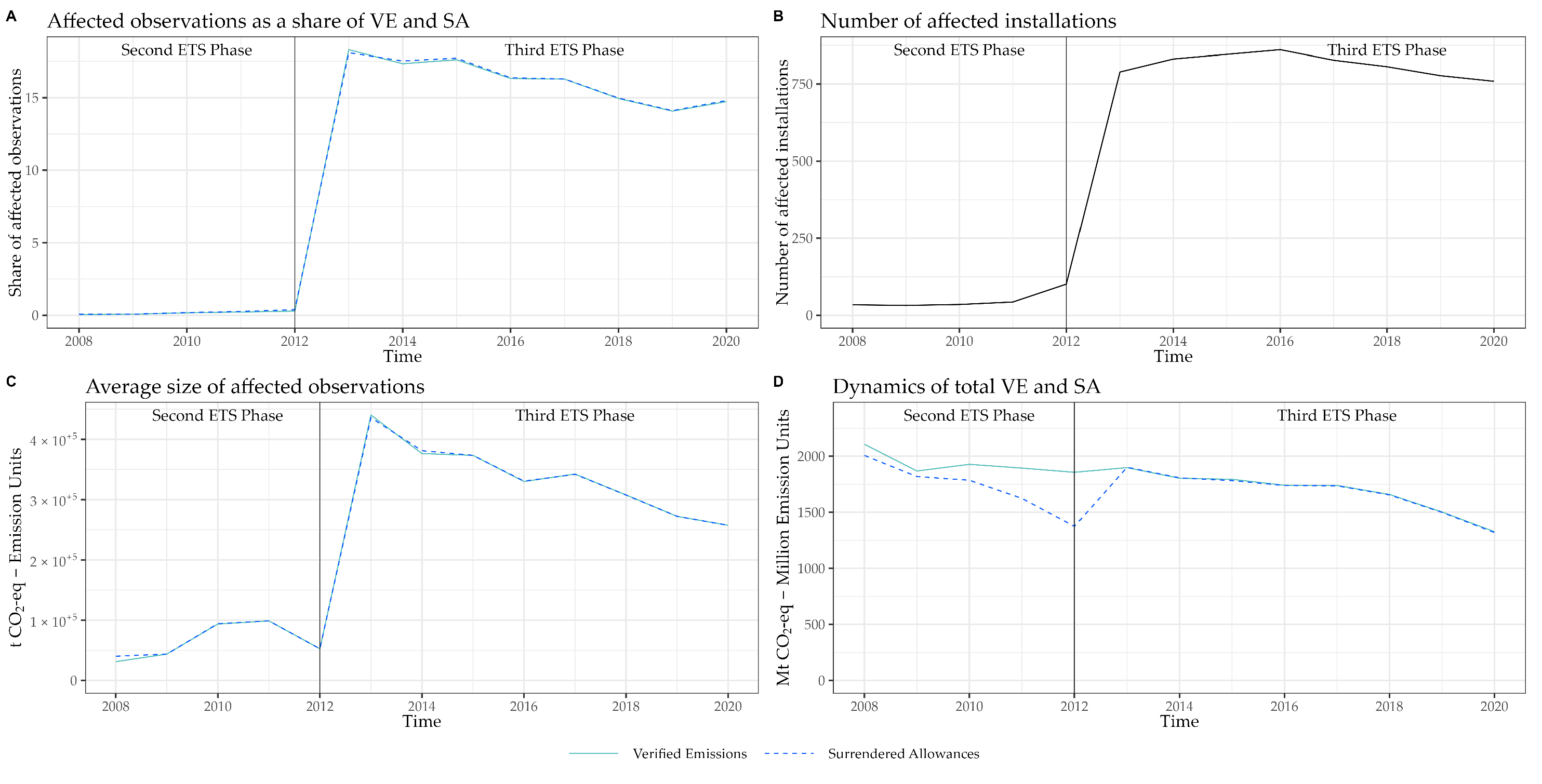
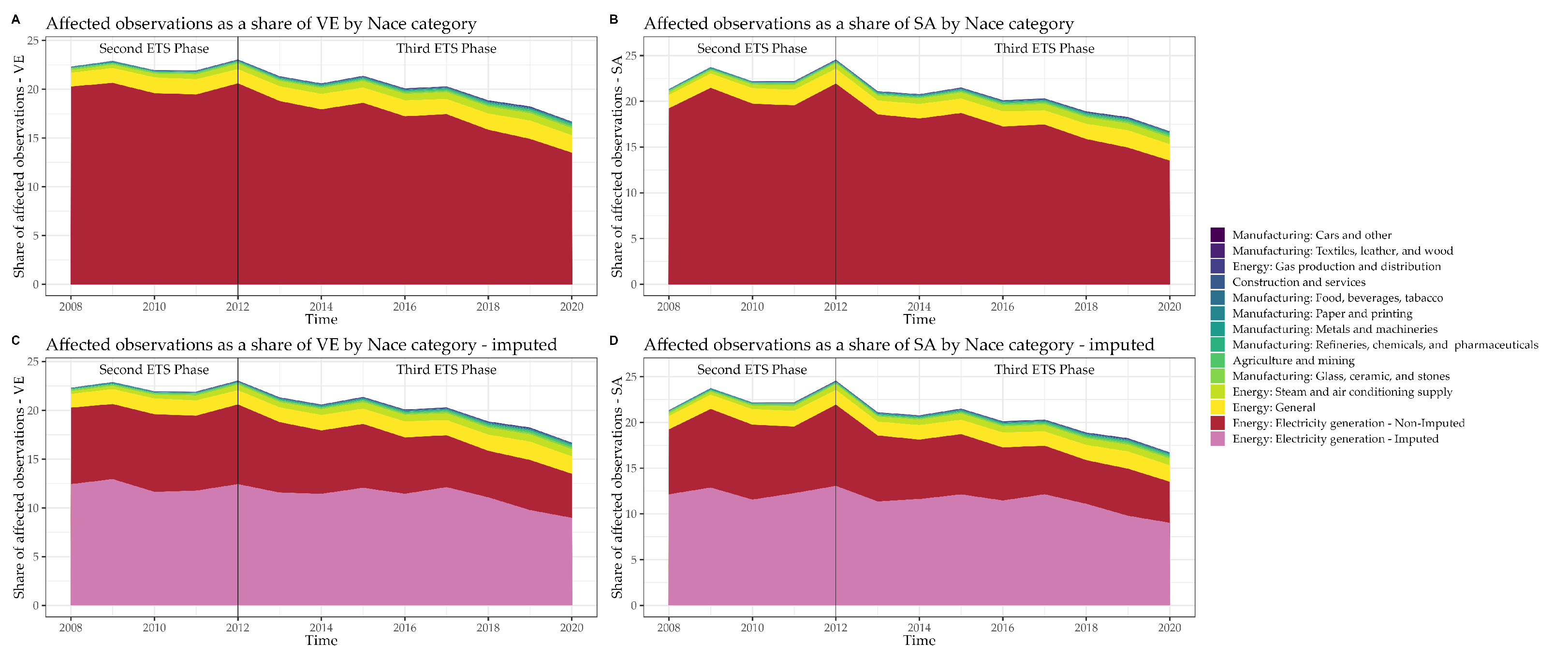
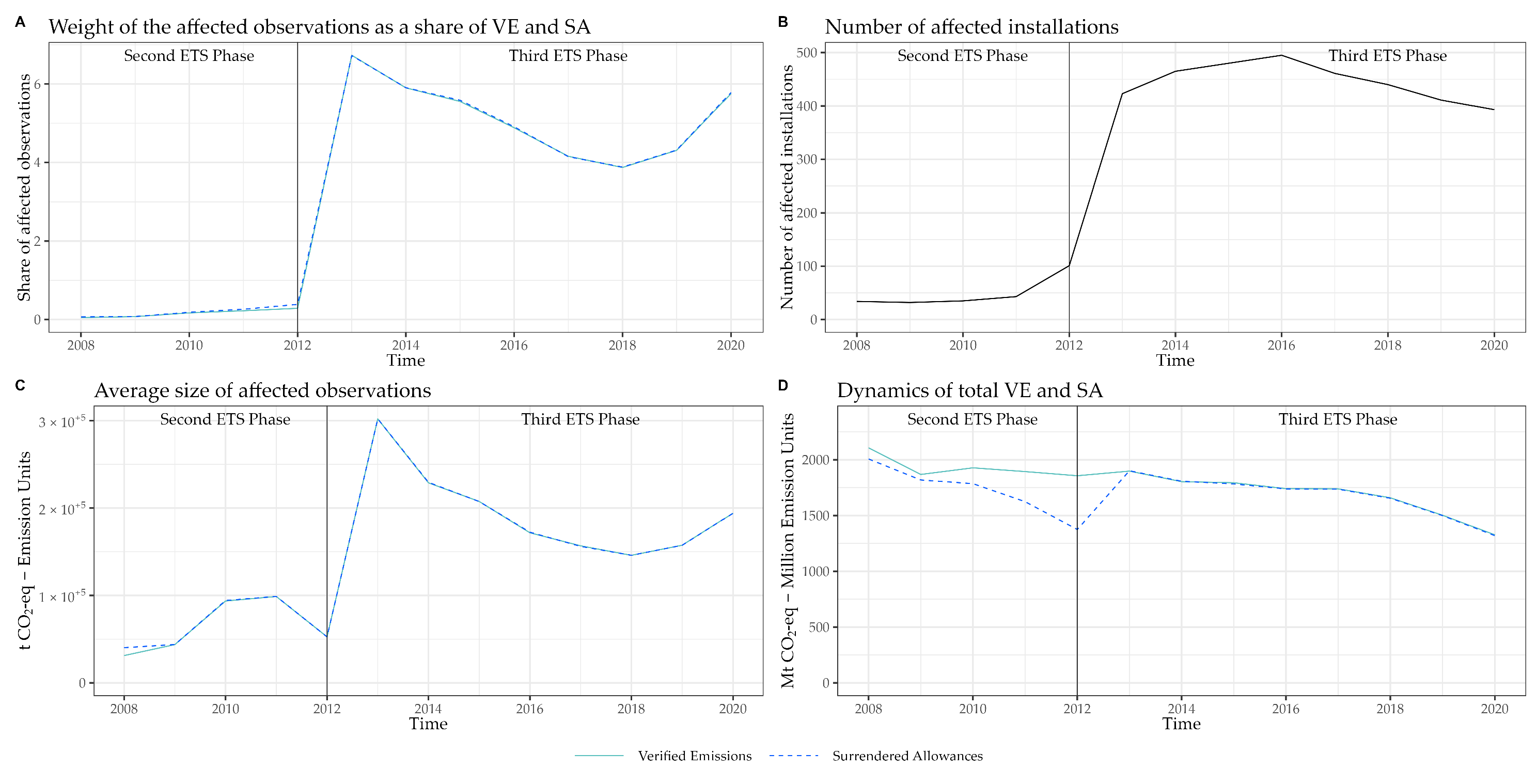
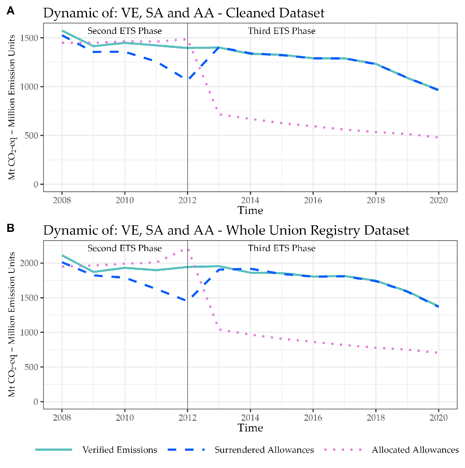
2.2. Datasets and Methodology

In this study, we exploit a panel dataset of yearly sector-by-country observations for the period 2008–2020 (Phases 2 and 3). Specifically, we use the Nace classification to analyze the two sectors accounting for the vast majority of CO2-eq emissions (≥98%) under the EU ETS: sector C (≈63%) “Manufacturing” and sector D (≈35%) “Electricity, gas, steam and air conditioning supply” (energy from now on).
Our primary data source is the European Union Transaction Log (EUTL). We selected the following variables: verified CO2-eq emissions (VE), surrendered allowances (SA), and freely allocated allowances (AA). To align the installation-level data from the Union Registry with the sector of activity used in the analysis, we used an imputation table (available at https://euets.info (accessed on 26 February 2023)) based on the proceedings of the stakeholder meeting on the preliminary carbon leakage list for Phase 4 of the EU ETS [30].
A careful imputation of the missing values was performed before the analysis. Indeed, we find that the observations reporting both VE and SA, but missing AA, were of negligible weight until 2012, representing less than 0.3% of the sample. However, this proportion surged to ≈16% with the onset of Phase 3 (further details on the data imputation process are provided in Appendix A). On the abrupt change in behaviour of missing observations, see in particular Figure A1 and the related discussion. The affected installations represent a sizeable share of both VE and SA (>20%) and an overwhelming majority (>88%) are in the Nace category “Energy: Electricity generation” (see Figure A2). We argue that the most likely explanation for the surge in the number and weight of observations reporting both VE and SA, but lacking AA, is that they stopped reporting AA (or that their AA was not recorded) because they were no longer entitled to free allocation in Phase 3. Our conjecture is supported by the evidence that a stark majority of affected installations are missing AA for the entire Phase 3 and belong to countries where derogation 10c does not apply (where free allocation to the energy sector is not allowed). Along this line of thought, we presume that in several instances the affected observation should be imputed a zero AA and apply the following imputation strategy:
  • Identify observations reporting VE and SA but not AA for the entire third phase.
  • Identify the observations of Step 1 that are in the Nace category “Energy: Electricity generation”.
  • Identify the observations of Step 2 that are not in a country granted derogation by Article 10c of the ETS directive.
  • Impute 0 to the AA variable in place of a missing value to the observations identified in Step 3.
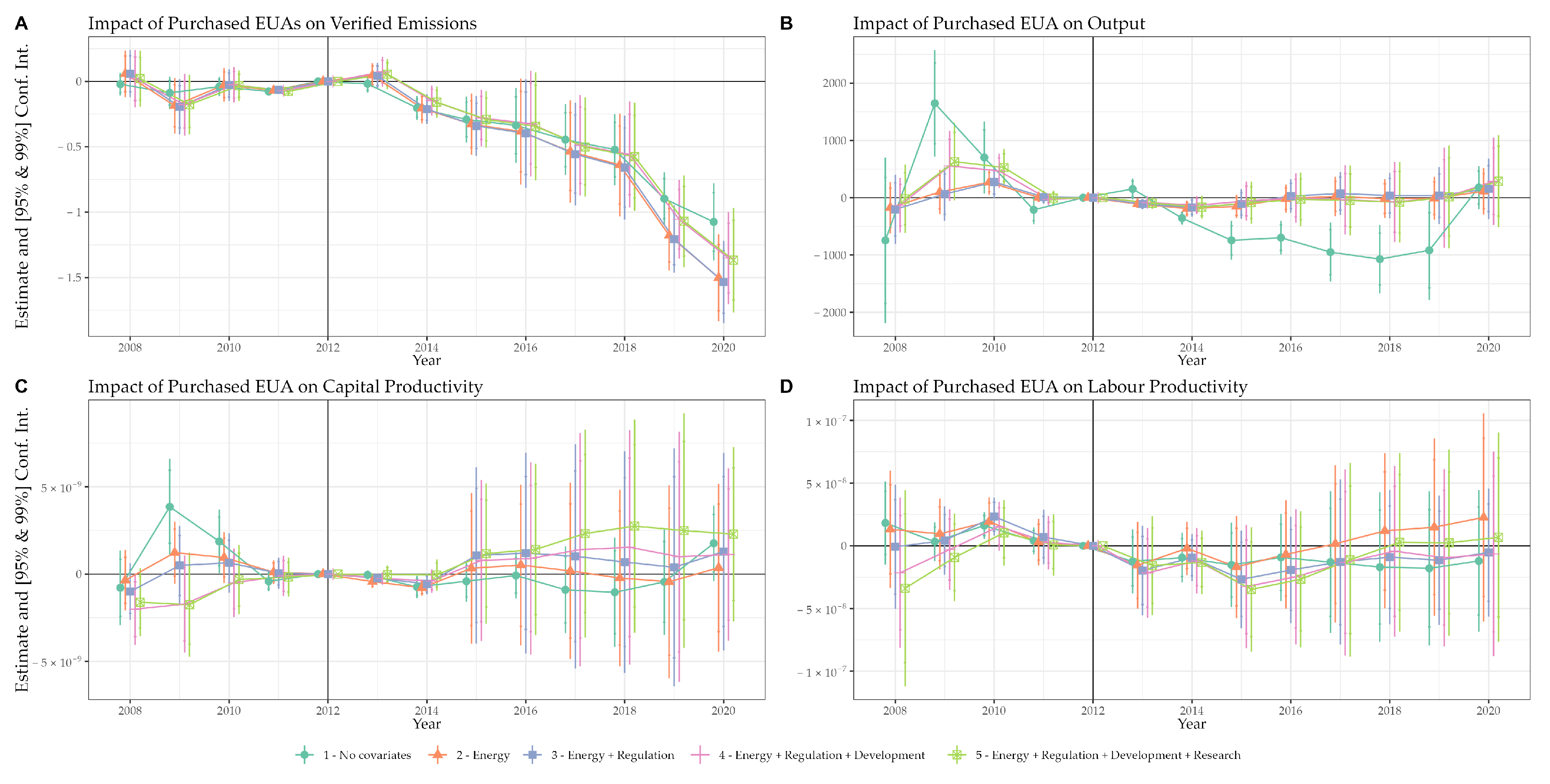
The total number of installations imputed is 366, with a decrease in the weight of the affected installations from ≈16% to ≈5% and a reduction of one-third of the average emissions of the observations affected (see Figure A3).
We argue that this imputation procedure brings the data closer to the real AA dynamic. Indeed, the installations subject to our imputation strategy are likely to be among the most affected by the policy change (high-emitters losing entirely the free allocation) and excluding them from the analysis would significantly—and mistakenly—reduce the estimated effect of the change in regulation. In support of this interpretation, we find that removing these observations from the dataset reduces the estimated impact of the treatment on emissions by ≈20%, although significance is not affected (the whole set of results without imputation is available on request).
We use the same policy evaluation techniques to investigate the impact of the EU ETS Phase 3 on emissions and performance. Here we outline these methods for the analysis regarding emissions, the extension to performance is straightforward.
To assess the impact of the EU ETS on emissions, it is crucial to determine if the emission dynamic was driven by regulation or other confounding factors. The ideal approach would be to compute the difference between observed emissions of installations under the new regulation against the emissions of the same installations under no change in regulations. Although this latter scenario is unobservable, econometric techniques can be used to approximate it. Our first method is an event study (ES) design, which enables the evaluation of the effect of a policy change on the variable under study over time. In the case of emissions, VE is the dependent variable while the policy change is represented by the implementation of Phase 3 in 2013. To determine the impact of the policy change on emissions, we compare the intensity of EU ETS regulations across installations, under the assumption that installations more heavily affected by regulations will have larger responses. Exploiting the observed differences in responses, we aim to estimate the regulation’s effect on emissions.
Using data from the EUTL, we define the variable Purchased EU Allowances (PEUA) as the difference between SA and AA. PEUA are a measure of the strength of the monetary incentives imposed by the EU ETS regulation on an installation (the exploitation of the variation between emissions and freely allocated EUA has been explored already in the literature [6,9,31]). In certain instances, particularly during Phase 2, there has been an excess of freely allocated emissions relative to verified emissions. This circumstance led to negative PEUA values. Consequently, in these cases installations receive a financial subsidy for emitting CO2, creating an incentive for increased emissions. In any case, economic rationality predicts that an increase of PEUA by an installation should induce a reduction of VE.
Due to the potential endogeneity arising from regulators’ decisions to treat emitters based on past behaviour, we set the treatment variable for each year at the median in Phase 2 (using the 2008 value does not alter significantly the results). Given the decrease in allowances allocated for free between Phase 2 and Phase 3, our treatment variable likely underestimates the impact and our findings should be considered a conservative lower bound of the true effect. Notice, however, that the adoption of the median value of PEUA in Phase 2 as a treatment implicitly assumes proportional treatment across years.
Equation (1) describes the event study specification [32] for sector-by-country observation i where the treatment year is identified by a dummy variable measuring the time to Phase 3 implementation 1 t t * = y with t * = 2013 (i.e., “event time”), and the intensity of treatment is measured by the (continuous) value of median PEUA in 2008–2012 P E U A i :
V E i t = P E U A i y = 5 2 ρ y 1 t t * = y + y = 0 7 λ y 1 t t * = y + γ X i , 2008 + θ t + η i + e i t
The event study methodology is a panel (2008–2020) regression of sector-by-country verified emissions ( V E i t ) (the dependent variable) over a measure of the treatment ( P E U A i ) interacted with year dummies, while controlling for other covariates that might affect emissions ( X i , 2008 ). We are especially interested in the coefficients ρ y and λ y that provide an estimate of the (covariate-adjusted) linear dependence of emissions from P E U A i in Phase 2 and Phase 3. Estimates are normalized to the year before the shift from Phase 2 to Phase 3 ( y = 1 , the year 2012). The resulting estimated set of coefficients, one for each year, measures the impact of the treatment on emissions. A negative coefficient implies that in that year, the emissions decrease induced by the treatment has been bigger than in the base year (and vice-versa). We cluster the standard errors at the country level to account for potential correlation within sectors of the same country. The obvious concern with event studies is the violation of the common trend assumption. To investigate the reliability of this assumption, ρ y can be used as a falsification test. Indeed, a lack of significance and a constant dynamic of the ρ y coefficients suggests that observations subject to different treatment intensities share a similar trend during the pre-treatment period. The λ y estimate intention-to-treat (ITT) effects and they measure, for each year of Phase 3, the impact on emissions of an additional median PEUA in Phase 2.
Our empirical strategy relies only on the parallel trends assumption, thereby obviating the need for balancing the levels of characteristics across observations subjected to varying degrees of treatment (as in methods relying on randomization). Notwithstanding, to control for differential treatment effects that might arise based on baseline country-sector characteristics, we incorporate a battery of baseline sector-by-country and country covariates interacted with year dummies X i , 2008 .
The variables used to this end are related to (i) energy consumption—energy use (Eurostat, see Appendix A for details on the imputation of the Nace sector to energy data), cooling and heating degree days (Agri4Cast); (ii) regulation—environmental taxes net of ETS revenues as a per cent of GDP (Eurostat) (https://ec.europa.eu/eurostat/statistics-explained/index.php?title=Tax_revenue_statistics, accessed on 30 March 2023), taxes on corporations (Eurostat), government expenditure as a per cent of GDP (Eurostat); (iii) development–labour hourly compensation (Eurostat), capital (Eurostat); (iv) innovation–intramural R&D expenditure as a per cent of GDP (Eurostat), GERD and BERD (Eurostat), total R&D personnel and researchers (Eurostat).
Furthermore, the fixed-effects panel approach used in the analysis also includes a set of year dummies θ t that absorbs temporal shocks and a set of sector-by-country dummies (the fixed effects η i ) that absorbs any time-constant characteristic at the observation level, such as regulation and social capital.
Equation (2) describes our difference-in-difference (DD) specification including an indicator variable that is equal to one during Phase 3, and the same treatment variable used in the ES specification, P E U A i . The model used in DD is as follows:
V E i t = β 1 1 t t * > 0 + β 2 P E U A i + β 3 P E U A i × 1 t t * > 0 + β 4 t X i , 2008 + θ t + η i + e i t
The variable 1 t t * > 0 indicates if the year belongs to Phase 3 of the EU ETS and its coefficient, β 1 , tells us whether the years in Phase 3 saw a change in the outcome analyzed; the variable P E U A i is our treatment variable and the associated coefficient β 2 captures differences in levels of the outcome V E i t between observations subject to different intensity of treatment. Our parameter of interest is β 3 , the coefficient of the interaction term P E U A i × 1 t t * > 0 , that estimates the mean additional reduction in CO2-eq emissions for the period 2013–2020 that is induced by an additional median PEUA in Phase 2 when passing from Phase 2 to Phase 3 of the EU ETS.
Through Article 10c of the EU ETS Directive, lower-income Member States had the opportunity to grant free allocation to electricity-generating installations during Phase 3 to support modernization investments. To assess the impact of this derogation on the effectiveness of the EU ETS, we implement a triple difference (DDD) design. This heterogeneity analysis is performed by including a binary variable 1 D e r o g , that indicates whether the country-sector falls under the derogation offered by article 10c, and its interactions with the variables 1 t t * > 0 , P E U A i and P E U A i × 1 t t * > 0 . The coefficient of interest of this specification, the one of the triple interaction term 1 D e r o g × P E U A i × 1 t t * > 0 , measures the differential impact on VE emissions in 2013–2020 induced by an additional median PEUA in Phase 2 for observations granted/not-granted by the derogation of Article 10c. A positive value of this coefficient would indicate a lower efficacy of the EU ETS for countries under derogation relative to those that were not granted the derogation.
Our analysis of performance aims to evaluate the impact of the tighter regulation of Phase 3 on the output produced and on the productivity of the inputs: capital and labour. We measure the output as the gross domestic product (GDP) of a sector-country at PPP. Capital productivity is measured as GDP per euro of capital in net fixed assets (at current replacement cost) while labour productivity is measured as GDP per euro spent on labour.
Eurostat national accounts do not explicitly report GDP at the sectoral level. We computed sectoral GDP by first identifying taxes and subsidies and then subtracting them from the sectoral gross value added. Capital productivity is obtained by dividing sectoral GDP by sectoral net fixed assets as reported by Eurostat. The total cost of labour by sector is computed as the number of hours worked times the nominal per-hour compensation of labour (adjusted for inflation and purchasing power). Labour productivity was then computed as the ratio of GDP over the cost of labour.
The analysis of performance is carried out using these three measures as dependent variables in the policy evaluation setting outlined above for the case of emissions.

3. Results

The EU ETS reform from Phase 2 to Phase 3 exposed different sector-by-country to a differential treatment intensity that we proxy using purchased EUA. In this section, we estimate the impact of the reform on CO2-eq emissions and performance measuring the differences in outcomes stemming from the difference in treatment intensity.

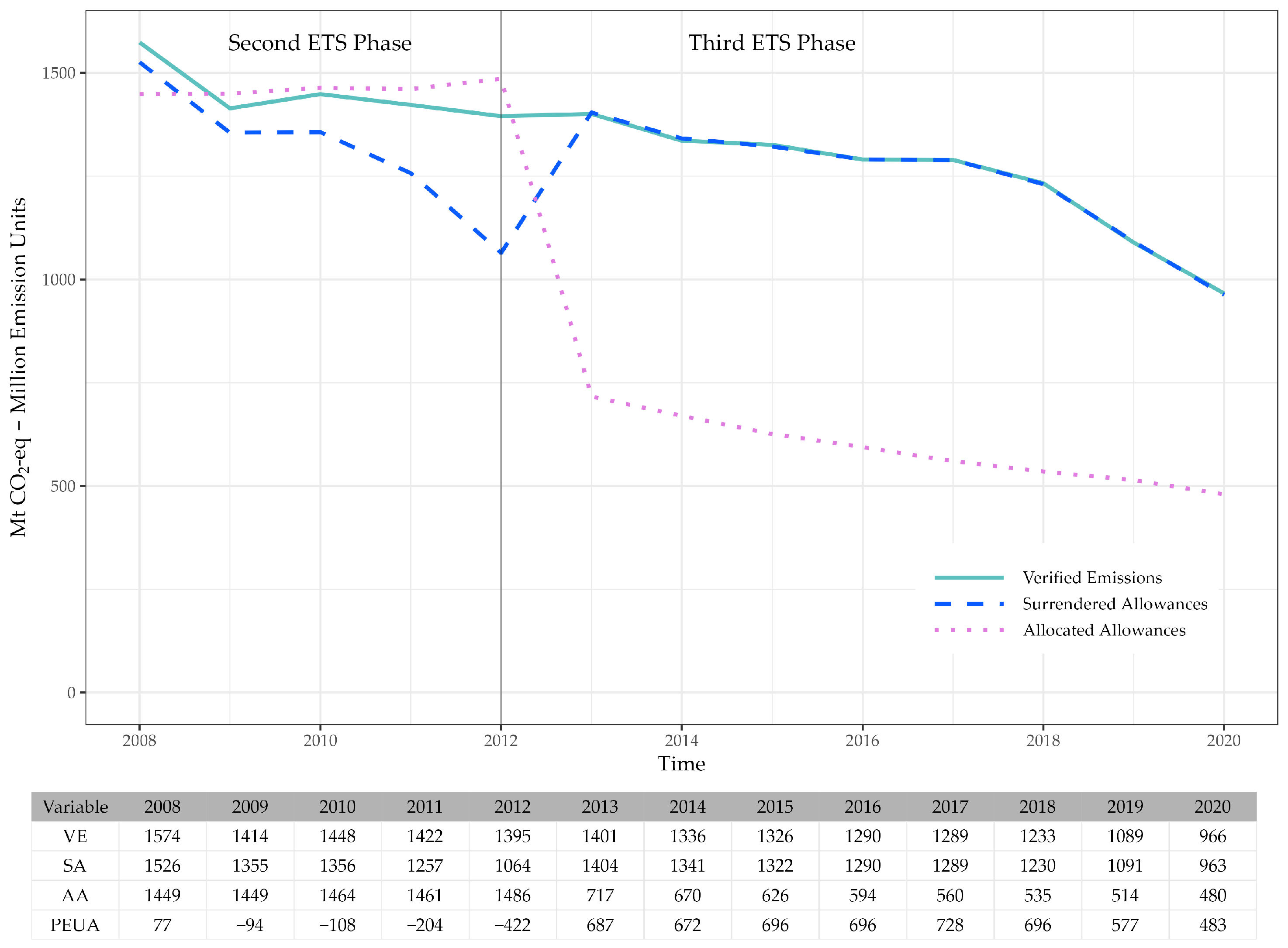
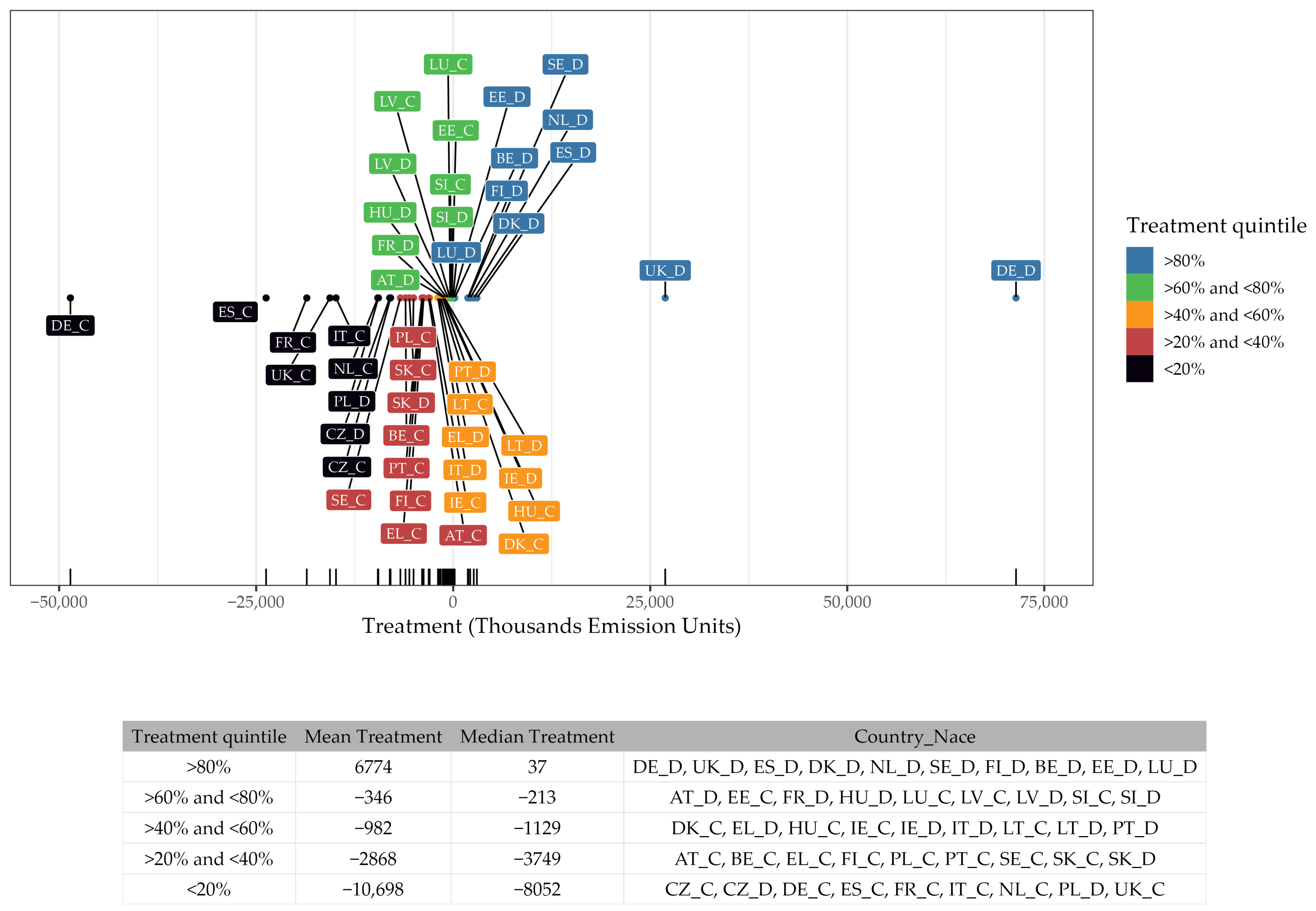
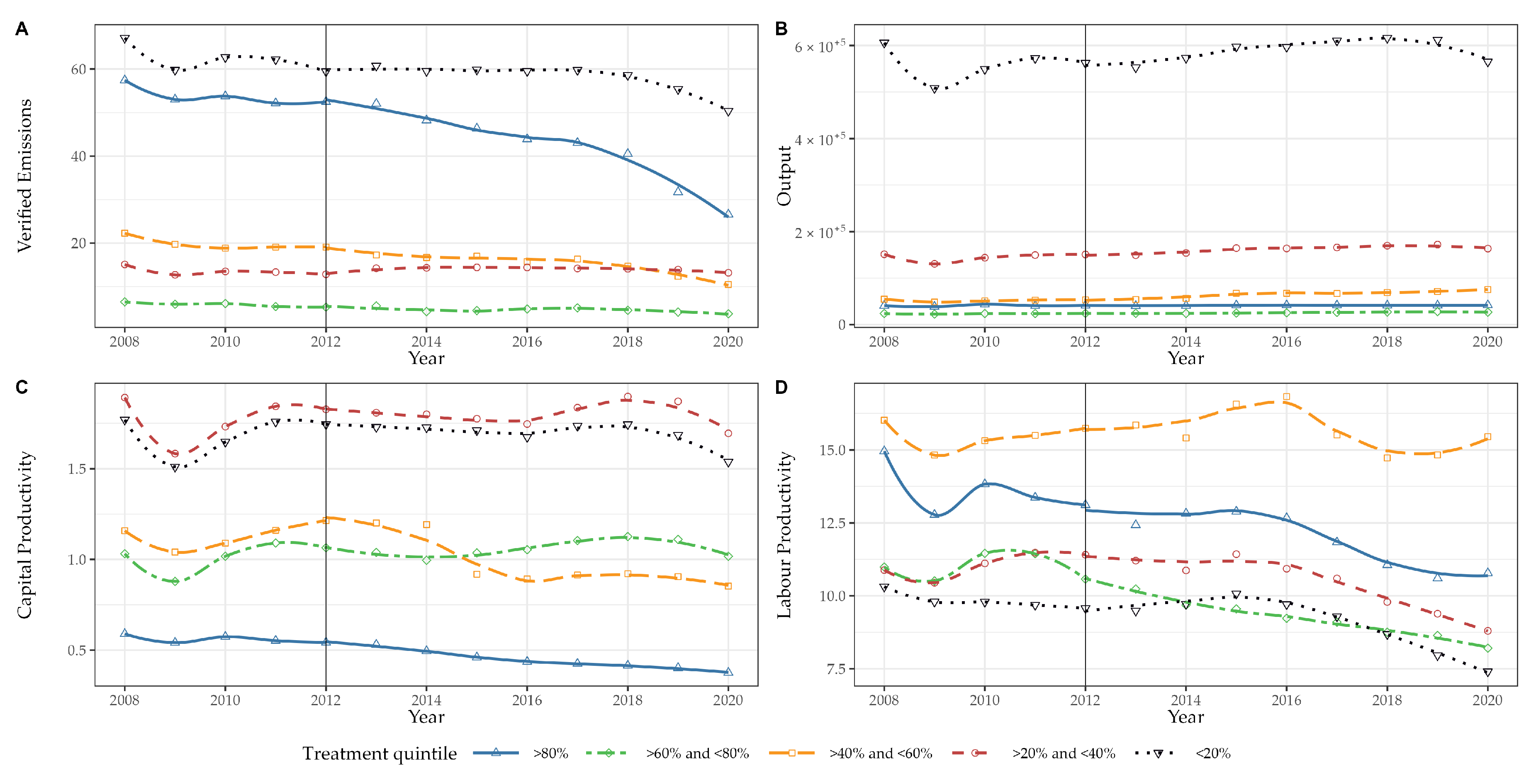
3.1. Descriptive Evidence

Before presenting the policy evaluation study, we report some descriptive evidence on our variables of interest and on our treatment. Figure 1 displays the evolution of the key variables of the European Union Registry from the cleaned sample (Our sample is ≈25% smaller relative to the EU ETS registry due to data cleaning. However, the dynamics of the variables in the two datasets are substantially the same, see Figure A4). The solid cyan line represents the evolution of total verified emissions, exhibiting a moderate downward trend that becomes more pronounced starting in 2018. Total surrendered allowances (dashed blue line) are consistently below VE during Phase 2, with a growing discrepancy over time. However, starting with the first year of Phase 3, SA closely matches VE, suggesting a tightening of the enforcement of the EU ETS regulations. The evolution of total freely allocated allowances (dotted pink line) mostly tracks the verified emissions in Phase 2, albeit with a sizeable over-allocation at the end of the phase. At the beginning of Phase 3, AA plummets (due to the shifting towards auction allocation) and then sets on a moderately decreasing trend. As a consequence, purchased EU Allowances experienced a significant increase from Phase 2 to Phase 3, due to both the stricter enforcement (rise in SA) and the reduction in free allocation (decline in AA). As illustrated by the final row in the table presented in Figure 1, the average PEUA was −150 during Phase 2, but it increased to 654 during Phase 3.
Information on the distribution of our treatment ( P E U A i ) is reported in Figure 2, where it is apparent that sector D is characterized by a higher intensity relative to sector C where lower, and generally negative values, are observed. From the figure, we can also see that the treatment is quite concentrated at zero, albeit with significant outliers in both directions. In general, more developed countries tend to occupy the extreme on the right with their D sector and the extreme on the left with their C sector, suggesting a widespread over-allocation of EUA in the latter sector during Phase 2. Notably, the only quintile with positive treatment (both average and median) is the top one.
In Figure 3, we illustrate the dynamic of the outcomes of interest, emissions and performance, by quintiles of the treatment. Interestingly, panel A shows that the evolution of verified emissions for all quintiles is constant or slightly decreasing during 2008–2012, casting a favourable outlook on the assumption of parallel trends before treatment, crucial to our policy evaluation exercise (event study–ES, difference-in-difference–DD, and triple difference—DDD). As the panel shows, there is a heterogeneous dynamic across treatment quintiles, with the top one, and in a lesser measure the third, displaying a more marked reduction in emissions at the onset of Phase 3. Conversely, the other quintiles show no discernible change in trend after 2013. Based on this descriptive evidence, it appears that buying EUA may have had a significant impact on reducing emissions, while the role of overallocation seems limited. Panels B, C, and D show the evolution of the measures of performance: output, capital productivity, and labour productivity. The panels display more variable dynamics and also a more marked heterogeneity across quintiles relative to panel A during Phase 2. While panel B shows a very low heterogeneity across quintiles during the whole period, panels C and D display more variability, but no significant change seems to occur between Phases 2 and 3.
We use standard causal inference methods to investigate this descriptive evidence rigorously. Our empirical strategy exploits the panel nature of the data and does not require a balance in levels between observations under different treatment intensities. Nevertheless, observations with different baseline characteristics might undergo differential treatment effects, so we explore the distribution of variables that might be correlated with heterogeneity in treatment effects. In Table 1, we report the average value of each covariate by quantile and test for the presence of differences in mean. We can see that energy and capital are negatively correlated with the treatment quintile and that there are significant differences across quintiles. Furthermore, the top quintile is different from the others on several dimensions: labour hourly compensation, GERD, BERD, and R&D employees. The remaining covariates show no significant differences in means across quintiles.

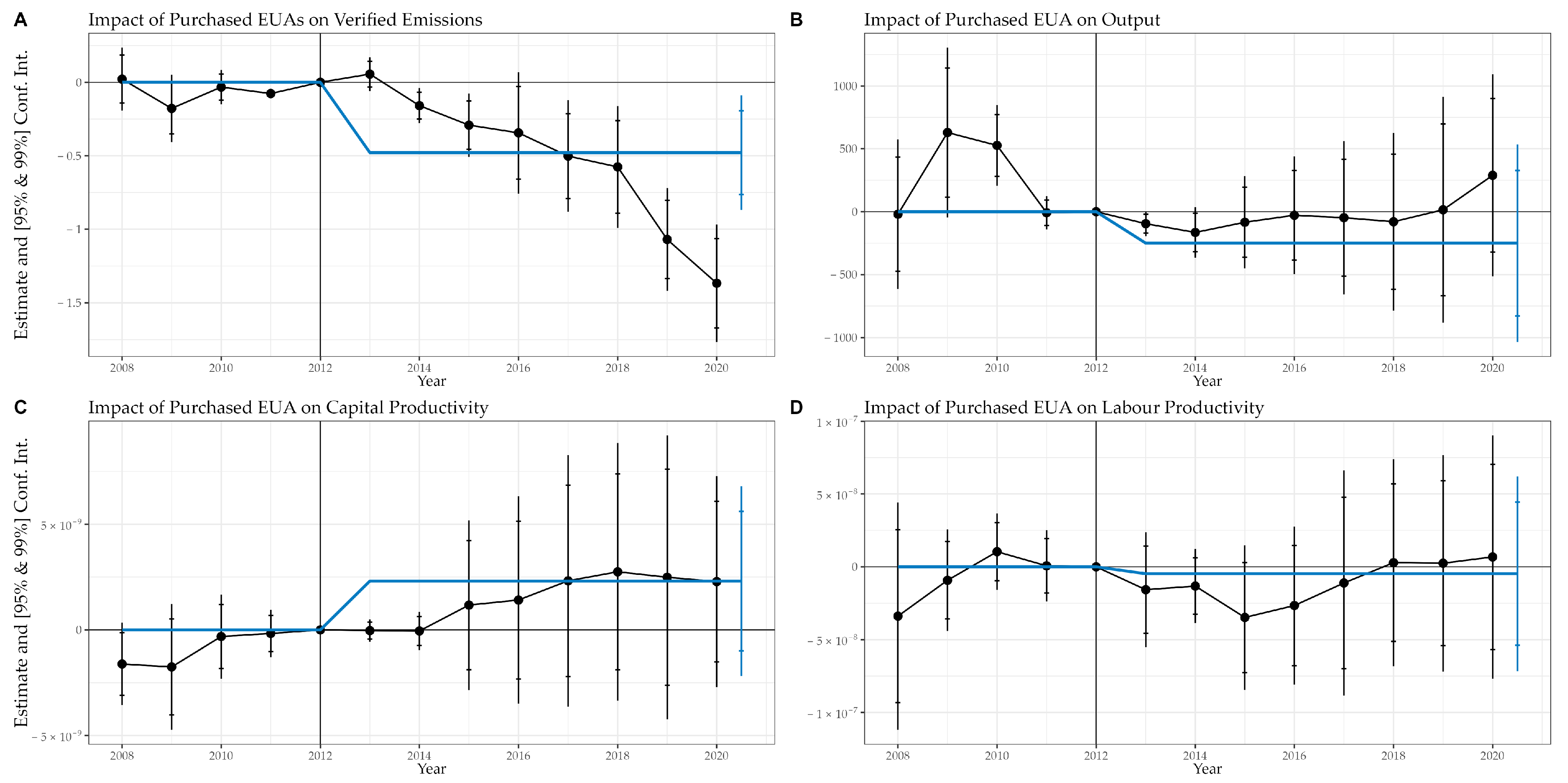
3.2. Policy Evaluation

Figure 4 illustrates in black the event study design, which showcases the progression of the coefficients ρ y and λ y for our four dependent variables of interest: verified emissions (panel A), output (panel B), capital productivity (panel C), and labour productivity (panel D). In Table A1 of Appendix B we report the key coefficients of the event study for all the dependent variables using the same panel names. For verified emissions, results during the pre-reform period are largely insignificant, apart from a small but statistically significant coefficient observed in 2011. Conversely, during Phase 3, all but two coefficients are highly significant at the 1% level, with large, negative, and diminishing values over time. The treatment coefficients for VE steadily decrease from zero in 2013 to −1.4 in 2020. The assumption of parallel trends during Phase 2 also holds for all the performance variables (see panels B, C, and D, of Figure 4 and Table A1), albeit with some evidence of higher output for more intensely treated observations during the years 2009 and 2010. All Phase 3 coefficients on panels B, C, and D are small and insignificant. For output, our analysis implies that an increase in P E U A i by one unit led to a decrease in output of around one hundred euros each year, which is comparable to the current cost of an allowance. The coefficients estimated for capital and labour productivity (panels B and D) are negligible for all practical purposes.
Figure 4 also illustrates in blue the treatment effect for the whole third phase, which we estimate using our DD specification. The 99% confidence interval for the VE coefficient is [−0.0896, −0.867] with a point estimate of −0.479 (see panel A, row DD of Table 2). This result implies that a unitary increase in median purchased allowances during Phase 2 led to a decrease of almost half a ton of CO2-eq emissions during Phase 3. The DD coefficients of the productivity variables, reported in panels B, C, and D of Table 2, are small and not significant.
Rows DDD of Table 2 present the results of our heterogeneity analysis that investigates the impact of the derogation to the EU ETS granted under article 10c of the ETS directive. Panel (A) shows the coefficient of Post × Treatment to be largely unaffected while the coefficient of the triple interaction term is large, positive, and highly significant (at the 1% level). The possibility granted to the less-developed Member States to freely allocate allowances to the installations of the energy sector in Phase 3 resulted in a large and significant increase in verified emissions. For the countries under Derogation 10c, an increase by one unit of P E U A i led to an increase of more than half a ton of CO2-eq. The triple interaction term for labour productivity (Panel D) is negative and significant at the 10% level but its magnitude is negligible. The DDD coefficients of the remaining performance variables are small and not significant. Although countries that were granted Derogation 10c took advantage of the relaxed emission constraint, this did not lead to an improvement in their performance; a finding suggesting that derogation 10c induced limited competitive distortions.
To further corroborate the validity of our finding on verified emissions, we first run a placebo event study whose results are reported in Figure A6, Figure A7 and Figure A8 of Appendix B. These placebo tests switch the dependent variable and the covariates one at a time. As covariates should not be impacted by P E U A i , we do not expect to observe any discontinuity in the estimated coefficients at the cutoff. Reassuringly, the estimated effects are small and statistically insignificant.
Furthermore, in Appendix B, Figure A5, we show that the ES results are robust to the inclusion of different sets of covariates. We report in Table A2 the analogous analysis on the DDD estimator. The DD table is omitted for brevity.

4. Discussion

The EU Emissions Trading System serves as a cornerstone in the achievement of the GHG emission reduction targets established in the 2020 climate and energy package and in the 2030 Climate and Energy framework. This study investigates the impact on CO2-eq emissions and on the economic performance of the tightening of the EU ETS regulation between Phases 2 and 3.
The extant empirical literature demonstrates the limited emission reduction efficacy of the EU Emissions Trading System in Phase 1 and the more marked, albeit limited, effects in Phase 2. In the first examination of Phase 3 in the literature, we show that tighter regulation of Phase 3, by increasing the purchased EUA, led to a statistically significant and sizeable reduction of emissions relative to Phase 2. An additional median purchased allowance in Phase 2 ( P E U A ) reduced verified emissions in Phase 3 by half a ton. This implies that incentives within the EU ETS are significantly enhanced when companies are required to purchase allowances, rather than having them allocated for free.
We can use our estimates to quantify the total amount of CO2-eq reduction achieved during Phase 3 as a result of the increase in purchased EUA induced by the tightening of the EU ETS regulation. To carry out this exercise, we multiply the difference between median allowances allocated for free during the pre-treatment (Phase 2) and the post-treatment (Phase 3) by the estimated coefficient β ^ 3 of Equation (2). Using a 5% confidence interval on β ^ 3 , the reduction in CO2-eq emissions ranges between −675 and −170 Mt, with a point estimate of −422 Mt. The reduction is substantial, around 4.3% of Phase 2 emissions (21.6% of the average year) and 3.0% of Phase 3 emissions (24.1% of the average year) in our sample. Notably, this is a conservative appraisal of the impact of the EU ETS since it is just accounting for the differential impact of P E U A (excluding the baseline).
The scientific literature presents very limited evidence of a detrimental effect of the EU ETS on performance during Phases 1 and 2, potentially due to positive innovation developments. Despite the increase in strictness in Phase 3, our results also show no sign of an adverse impact on performance.
Our analysis reveals heterogeneity in the EU ETS effect across countries, with those allowed to provide a free allocation of allowances to energy installations (under the derogation provided by Article 10c of the ETS Directive) experiencing an increase in emissions of half a ton for each additional P E U A . However, we find no evidence of a relative improvement in performances for countries under Derogation 10c. These findings warn against the adverse impact of derogations to the ETS system on emissions while softening the concerns regarding the competitive distortions induced by the regulation. Given the reduction in emissions and the lack of a detrimental impact on performance, our investigation sheds a favourable light on the additional reduction of the free allocation of allowances entailed by Phase 4.
The identification strategy proposed in this study compares European country-sectors that have been induced to purchase different amounts of EUA and that were/were not eligible for Derogation 10c. Hence, our estimations do not entail a comparison of the performance against non-European counterparts. Based on the findings here presented, it appears unlikely that the change in the regulation of the EU ETS led to a performance decline compared to non-European competitors. However, further research to delve deeper into this issue is recommended. Our study leaves open several other key areas of inquiry, particularly on the technological and organizational changes that allowed a reduction of emissions without losses in performance and on the impact of EUA prices in inducing emission reductions. On this latter point, in the current analysis we used quantities of EUA to measure economic incentives induced by the tighter regulation of Phase 3. An even better measure would have been the cost of the purchased EUA, but endogeneity concerns prevented its utilization. Several aspects of the EU ETS regulation implemented in Phase 4 (and currently under discussion) will be affecting companies’ decisions by raising the price of EUA (e.g., the Market Stability Reserve). Hence, we strongly believe that further research focused on evaluating the impact of EUA prices using sources of exogenous variation would provide key insights for future scientific and policy debate.

Author Contributions

M.B. and D.G.d.I. contributed equally to the manuscript. All authors have read and agreed to the published version of the manuscript.

Funding

This research received no external funding.

Institutional Review Board Statement

Not applicable.

Informed Consent Statement

Not applicable.

Data Availability Statement

Data on emissions and EUA have been scraped from the EUTL registry using the code in this repository https://github.com/dgdi/EUTL_OHA_data (accessed on 30 March 2023). The rest of the data is freely available on the EUROSTAT database website https://ec.europa.eu/eurostat/data/database (accessed on 30 March 2023) and on the Agri4Cast database https://agri4cast.jrc.ec.europa.eu/dataportal/ (accessed on 30 March 2023).

Acknowledgments

This paper builds on a preliminary analysis that we developed in the context of a CIFREL study for the EU Parliament [33]. The authors would like to extend their sincerest gratitude to M. Buso, R. Caruso, L. Gerotto, R. Levaggi, L. Rizzo, R. Secomandi, and G. Turati for their valuable comments and discussions on an earlier version of this draft. The authors would also like to acknowledge the valuable insight provided by D. Cipullo, T. Colussi, E. Rettore and L. Salvadori on the policy evaluation design.

Conflicts of Interest

The authors declare no conflict of interest.

Abbreviations

The following abbreviations are used in this manuscript:
AAFreely allocated allowances
DD       Difference-in-difference
DDDTriple difference
ESEvent study
EU ETSEuropean Union Emissions Trading System
EUTLEuropean Union Transaction Log
EUAEuropean Union Allowances
PEUAPurchased EUA
SASurrendered allowances
VEVerified emissions

Appendix A. Data

Panel A of Figure A1 shows the sudden and dramatic increase in the weight of observations reporting VE and SA but missing AA at the onset of Phase 3. The dynamic of this increase can be decomposed into three parts: (i) a significant rise in the number of installations no longer reporting AA (panel B), from about 50 in the 2008–2012 period to around 800 in the 2013–2020 window; (ii) a pronounced increase (more than three-fold) in the average values of VE and SA of the observations (panel C), pointing to a shift towards high-emitting installations; (iii) a decreasing trend in both VE and SA levels, as illustrated in panel D.
Figure A1. Observations with available VE and SA but missing AA during Phases 2 and 3—before imputation. (A) Affected observations as a share of VE and SA; (B) Number of affected installations; (C) Average size of affected observations; (D) Dynamic of total VE and SA.
Sustainability 15 06394 g0a1
The dynamic of VE and SA of the affected installations, those that in at least one year report both VE and SA but lack AA, is plotted in panels A and B of Figure A2. In panels C and D of the same figure we illustrate the dynamic of VE and SA of installations subject to imputation.
Figure A2. Observations with available VE and SA but missing AA by Nace category during Phases 2 and 3. (A) Affected observations as a share of VE by Nace category; (B) Affected observations as a share of SA by Nace category; (C) Affected observations as a share of VE by Nace category and imputation status; (D) Affected observations as a share of SA by Nace category and imputation status.
Sustainability 15 06394 g0a2
Figure A3 replicates Figure A1 after the imputation.
An additional imputation procedure for the EU registry data was implemented to exploit the information contained in the “Compliance_Code” variable. When the value of “Compliance_Code” is “A” the installation is compliant in that year, meaning that the SA covers the VE. For any observation where either SA or VE is missing and “Compliance_Code” is “A”, the missing value is imputed based on the available value. As a robustness check, we also performed the analysis without this imputation step, the impact on results is negligible.
Figure A3. Observations with available VE and SA but missing AA during Phases 2 and 3—after imputation. (A) Affected observations as a share of VE and SA; (B) Number of affected installations; (C) Average size of affected observations; (D) Dynamic of total VE and SA.
Sustainability 15 06394 g0a3
The energy data (from the energy balances Eurostat dataset) are imputed to Nace sectors following the Energy Balance Guide [34], the Manual for Air Emissions Accounts [35], and the Validation rules for Air Emissions Accounts [36]. To validate our findings, we also devised an alternative, less-conservative specification of the energy variable by following the International Recommendations for Energy Statistics [37]. Specifically, we employed a residual imputation technique to address any gap in our energy data. Our results are robust to the imputation method (imputation tables and the associated results are available upon request).
Below we compare the dynamic of VE, SA and AA during Phases 2 and 3 for our cleaned sample (panel A, the plot is the same as the one in Figure 1) and the whole Union Registry dataset (panel B). While the whole dataset is more comprehensive, covering approximately 25% more emissions/units, the qualitative dynamics of the two are remarkably similar.
Figure A4. Dynamic of total verified emissions, surrendered allowances, (freely) allocated allowances and purchased EUA during Phases 2 and 3 of the EU ETS for the cleaned dataset used in our analysis (panel A) and the whole EU ETS dataset (panel B).
Sustainability 15 06394 g0a4

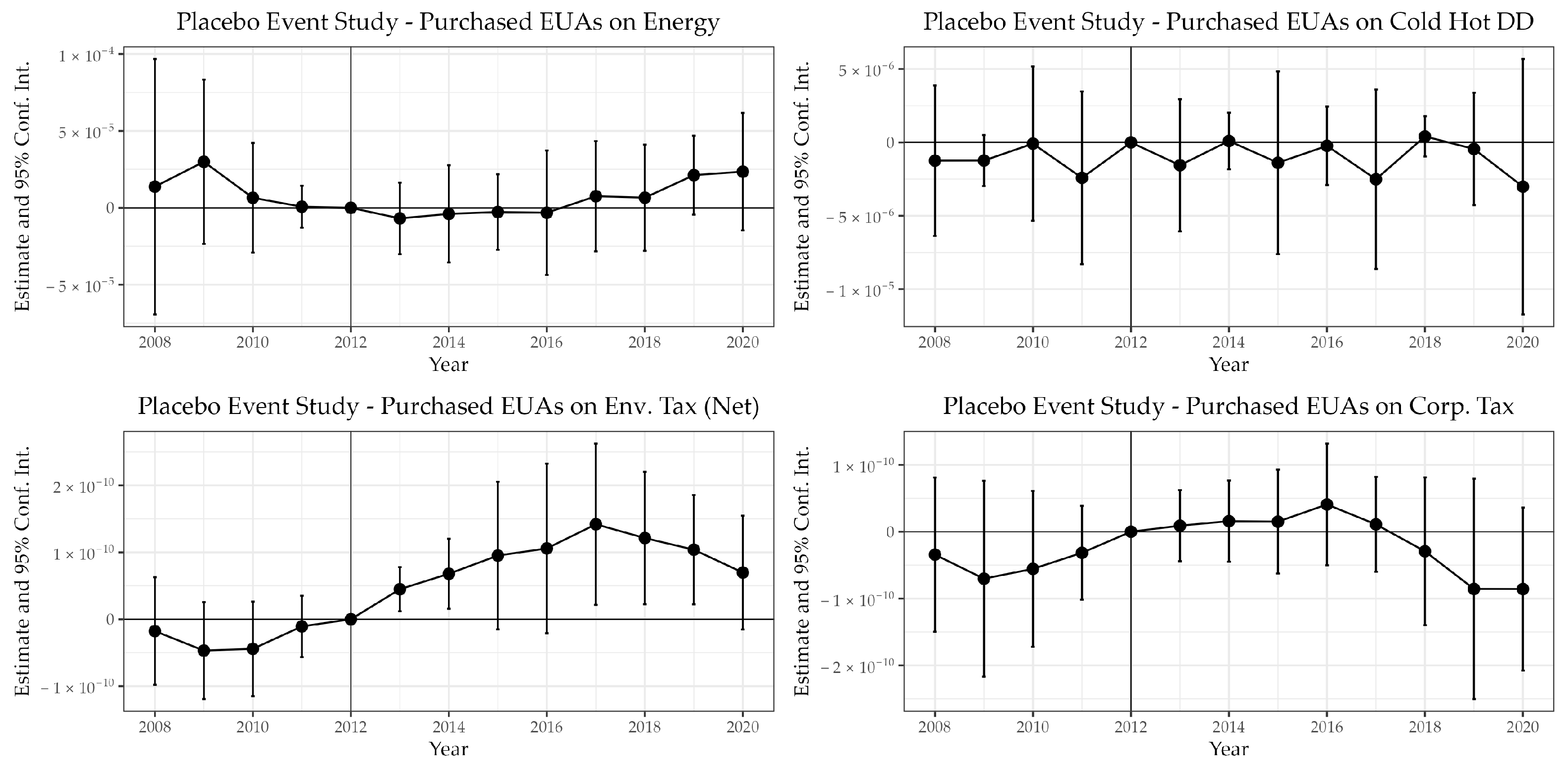
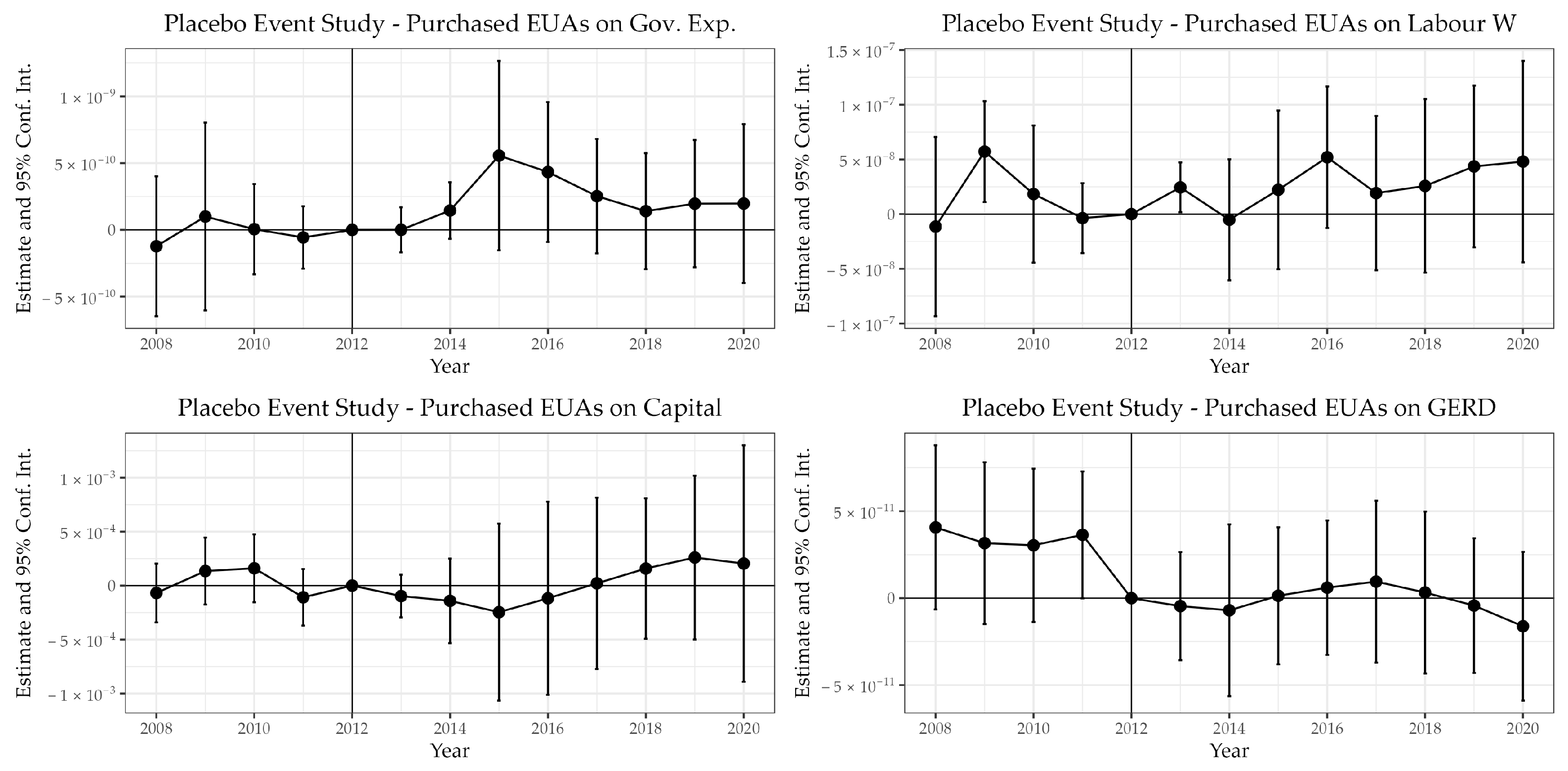
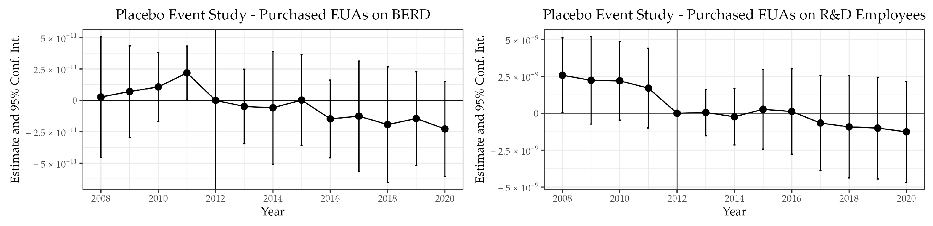
Appendix B. Policy Evaluation

Here we report the table with ES coefficients for all the dependent variables considered.
Table A1. Event study coefficients—verified emissions (A), output (B), capital productivity (C), and labour productivity (D).
Verified EmissionsOutputCapital ProductivityLabour Productivity
(A)(B)(C)(D)
Treatment × 20080.0216−19.75 1.61 × 10 9 ** 3.39 × 10 8
(0.0832)(231.3)( 7.56 × 10 10 )( 3.03 × 10 8 )
Treatment × 2009−0.1777 *629.5 ** 1.75 × 10 9 9.25 × 10 9
(0.0889)(262.2)( 1.16 × 10 9 )( 1.35 × 10 8 )
Treatment × 2010−0.0326526.9 *** 3.14 × 10 10 1.04 × 10 8
(0.0454)(124.9)( 7.72 × 10 10 )( 1.02 × 10 8 )
Treatment × 2011−0.0766 ***−8.188 1.69 × 10 10 6.83 × 10 10
(0.0112)(51.27)( 4.32 × 10 10 )( 9.52 × 10 9 )
Treatment × 20130.0557−95.26 ** 3.49 × 10 11 1.57 × 10 8
(0.0448)(38.14)( 2.03 × 10 10 )( 1.53 × 10 8 )
Treatment × 2014−0.1587 ***−164.9 ** 5.07 × 10 11 1.32 × 10 8
(0.0466)(77.74)( 3.5 × 10 10 )( 9.87 × 10 9 )
Treatment × 2015−0.2915 ***−83.95 1.17 × 10 9 3.48 × 10 8 *
(0.0839)(142.3)( 1.56 × 10 9 )( 1.93 × 10 8 )
Treatment × 2016−0.3439 **−28.27 1.41 × 10 9 2.66 × 10 8
(0.1606)(181.5)( 1.9 × 10 9 )( 2.1 × 10 8 )
Treatment × 2017−0.5021 ***−47.65 2.32 × 10 9 1.11 × 10 8
(0.1474)(236.9)( 2.31 × 10 9 )( 3 × 10 8 )
Treatment × 2018−0.5758 ***−79.70 2.75 × 10 9 2.83 × 10 9
(0.1608)(273.9)( 2.37 × 10 9 )( 2.76 × 10 8 )
Treatment × 2019−1.069 ***15.05 2.49 × 10 9 2.46 × 10 9
(0.1359)(348.3)( 2.61 × 10 9 )( 2.89 × 10 8 )
Treatment × 2020−1.367 ***289.0 2.28 × 10 9 6.77 × 10 9
(0.1553)(311.8)( 1.94 × 10 9 )( 3.24 × 10 8 )
X i , 2008
Country-Nace FE
Year FE
Observations559559559559
* p < 0.1, ** p < 0.05, *** p < 0.01.
Figure A5 illustrates the ES analysis with specifications including a progressively larger set of controls. Notably, all models show evidence in line with our preferred specification—model (5), presented in the main text. Model (2) includes the variables energy and cooling and heating degree days, model (3) adds environmental taxes net of ETS revenues, taxes on corporations and government expenditures, model (4) adds labour hourly compensation and capital and model (5) (the one presented in the main text) also includes intramural R&D expenditure (GERD and BERD) and total R&D personnel and researchers.
Figure A5. Event study—specifications with different sets of covariates. Estimated causal impact of purchased EUA on: verified emissions (A), output (B), capital productivity (C), and labour productivity (D).
Sustainability 15 06394 g0a5
Additionally, the results of the DDD analysis show limited sensitivity to the inclusion of controls:
Table A2. Triple difference—specifications with different sets of covariates. Estimated causal impact of purchased EUA and derogation status on Verified Emissions.
Verified Emissions
(1)(2)(3)(4)(5)
Post × Derog. 10c7,006,021.1 ***4,331,965.5 **9,866,287.5 **10,956,577.5 **14,199,090.8 **
(1,973,301.1)(1,909,609.4)(4,490,879.2)(4,566,324.7)(6,007,911.5)
Post × Treatment−0.4450 ***−0.5622 ***−0.5702 ***−0.4599 ***−0.4581 ***
(0.0844)(0.1322)(0.1214)(0.1070)(0.0973)
Post × Treatment × Derog. 10c1.353 ***1.250 ***1.335 ***0.9509 ***1.054 ***
(0.2528)(0.3080)(0.3648)(0.3246)(0.3432)
X i , 2008
Country-Nace FE
Year FE
Observations598598572559559
** p < 0.05, *** p < 0.01.
As a final robustness check, we report in Figure A6, Figure A7 and Figure A8 the placebo tests for the event study where the dependent variable is verified emissions. In particular, we use the event study specification including all covariates and switch the VE with the covariates one at a time. Note that when used as the dependent variable, the covariates vary in time (do not interact with the dummy for the year 2008). As expected, the figures show that P E U A i has no impact on control variables.
Figure A6. Placebo event study—panel 1.
Sustainability 15 06394 g0a6
Figure A7. Placebo event study—panel 2.
Sustainability 15 06394 g0a7
Figure A8. Placebo event study—panel 3.
Sustainability 15 06394 g0a8

References

  1. European Commission. Special Eurobarometer; Technical Report 459; European Commission: Luxembourg, 2017. [Google Scholar]
  2. European Parliamentary Research Service. Europe’s Two Trillion Euro Dividend: Mapping the Cost of Non-Europe, 2019–2024; Technical Report; European Parliamentary Research Service: Luxembourg, 2019. [Google Scholar]
  3. Martin, R.; Muûls, M.; Wagner, U.J. The impact of the European Union Emissions Trading Scheme on regulated firms: What is the evidence after ten years? Rev. Environ. Econ. Policy 2016, 10, 129–148. [Google Scholar] [CrossRef] [Green Version]
  4. Joltreau, E.; Sommerfeld, K. Why does emissions trading under the EU Emissions Trading System (ETS) not affect firms’ competitiveness? Empirical findings from the literature. Clim. Policy 2019, 19, 453–471. [Google Scholar] [CrossRef] [Green Version]
  5. Klemetsen, M.; Rosendahl, K.E.; Jakobsen, A.L. The impacts of the EU ETS on Norwegian plants’ environmental and economic performance. Clim. Chang. Econ. (CCE) 2020, 11, 2050006. [Google Scholar] [CrossRef]
  6. Carratù, M.; Chiarini, B.; Piselli, P. Effects of European emission unit allowance auctions on corporate profitability. Energy Policy 2020, 144, 111584. [Google Scholar] [CrossRef]
  7. Ellerman, A.D.; Buchner, B.K. Over-allocation or abatement? A preliminary analysis of the EU ETS based on the 2005–06 emissions data. Environ. Resour. Econ. 2008, 41, 267–287. [Google Scholar] [CrossRef] [Green Version]
  8. Anderson, B.; Di Maria, C. Abatement and allocation in the pilot phase of the EU ETS. Environ. Resour. Econ. 2011, 48, 83–103. [Google Scholar] [CrossRef] [Green Version]
  9. Abrell, J.; Faye, A.N.; Zachmann, G. Assessing the Impact of the EU ETS Using Firm Level Data; Bruegel Working Paper; Bruegel: Brussels, Belgium, 2011. [Google Scholar]
  10. Egenhofer, C.; Alessi, M.; Georgiev, A.; Fujiwara, N. The EU Emissions Trading System and Climate Policy towards 2050: Real Incentives to Reduce Emissions and Drive Innovation? Technical Report, CEPS Special Report; European Commission: Luxembourg, 2011. [Google Scholar]
  11. Petrick, S.; Wagner, U.J. The Impact of Carbon Trading on Industry: Evidence from German Manufacturing Firms. 2014. Available online: https://econpapers.repec.org/paper/zbwvfsc14/100472.htm (accessed on 30 March 2023).
  12. Wagner, U.J.; Muûls, M.; Martin, R.; Colmer, J. The causal effects of the European Union Emissions Trading Scheme: Evidence from French manufacturing plants. In Proceedings of the Fifth World Congress of Environmental and Resources Economists, Instanbul, Turkey, 28 June–2 July 2014. [Google Scholar]
  13. Jaraite, J.; Di Maria, C. Did the EU ETS make a difference? An empirical assessment using Lithuanian firm-level data. Energy J. 2016, 37, 1–23. [Google Scholar]
  14. Dechezleprêtre, A.; Nachtigall, D.; Venmans, F. The Joint Impact of the EuropeanUnion Emissions Trading System on Carbon Emissions and Economic Performance. J. Environ. Econ. Manag. 2023, 118, 102758. [Google Scholar] [CrossRef]
  15. Bel, G.; Joseph, S. Emission abatement: Untangling the impacts of the EU ETS and the economic crisis. Energy Econ. 2015, 49, 531–539. [Google Scholar] [CrossRef]
  16. Jaffe, A.B.; Peterson, S.R.; Portney, P.R.; Stavins, R.N. Environmental regulation and the competitiveness of U.S. manufacturing: What does the evidence tell us? J. Econ. Lit. 1995, 98, 853–873. [Google Scholar]
  17. Rose, A. Modeling the macroeconomic impact of air pollution abatement. J. Regul. Sci. 1983, 23, 441–459. [Google Scholar] [CrossRef]
  18. Joshi, S.; Lave, L.; Shih, J.S.; McMichael, F. Impact of Environmental Regulation on the U.S. Steel Industry; Technical Report; Carnegie Mellon University: Pittsburgh, PA, USA, 1997. [Google Scholar]
  19. Porter, M. America’s green strategy. Sci. Am. 1991, 264, 168. [Google Scholar] [CrossRef]
  20. Ambec, S.; Cohen, M.A.; Elgie, S.; Lanoie, P. The Porter hypothesis at 20: Can environmental regulation enhance innovation and competitiveness? Rev. Environ. Econ. Policy 2013, 7, 2–22. [Google Scholar] [CrossRef] [Green Version]
  21. Mazzucato, M. The Green Entrepreneurial State; Routledge: Abingdon, UK, 2015. [Google Scholar]
  22. Martínez-Zarzoso, I.; Bengochea-Morancho, A.; Morales-Lage, R. Does environmental policy stringency foster innovation and productivity in OECD countries? Energy Policy 2019, 134, 110982. [Google Scholar] [CrossRef] [Green Version]
  23. Jaraitė, J.; Di Maria, C. Efficiency, productivity and environmental policy: A case study of power generation in the EU. Energy Econ. 2012, 34, 1557–1568. [Google Scholar] [CrossRef] [Green Version]
  24. Chan, H.S.R.; Li, S.; Zhang, F. Firm competitiveness and the European Union emissions trading scheme. Energy Policy 2013, 63, 1056–1064. [Google Scholar] [CrossRef] [Green Version]
  25. Marin, G.; Marino, M.; Pellegrin, C. The impact of the European Emission Trading Scheme on multiple measures of economic performance. Environ. Resour. Econ. 2018, 71, 551–582. [Google Scholar] [CrossRef]
  26. Guo, J.; Gu, F.; Liu, Y.; Liang, X.; Mo, J.; Fan, Y. Assessing the impact of ETS trading profit on emission abatements based on firm-level transactions. Nat. Commun. 2020, 11, 2078. [Google Scholar] [CrossRef] [PubMed]
  27. Coase, R.H. The Problem of Social Cost. J. Law Econ. 1960, 3, 1–44. [Google Scholar] [CrossRef]
  28. Goulder, L.H.; Parry, I.W.; Williams III, R.C.; Burtraw, D. The cost-effectiveness of alternative instruments for environmental protection in a second-best setting. J. Public Econ. 1999, 72, 329–360. [Google Scholar] [CrossRef] [Green Version]
  29. Lise, W.; Sijm, J.; Hobbs, B.F. The impact of the EU ETS on prices, profits and emissions in the power sector: Simulation results with the COMPETES EU20 model. Environ. Resour. Econ. 2010, 47, 23–44. [Google Scholar] [CrossRef]
  30. European Commission, Directorate-General for Climate Action. Stakeholder meeting on the results of the preliminary carbon leakage list for phase 4 of the EU Emissions Trading System. In Commission Notice on the Preliminary Carbon Leakage List for the EU ETS for Phase 4 (2021–2030); European Commission: Luxembourg, 2018. [Google Scholar]
  31. Anger, N.; Oberndorfer, U. Firm performance and employment in the EU emissions trading scheme: An empirical assessment for Germany. Energy Policy 2008, 36, 12–22. [Google Scholar] [CrossRef]
  32. Jacobson, L.; LaLonde, R.; Sullivan, D. Earnings losses of displaced workers. Am. Econ. Rev. 1993, 83, 685–709. [Google Scholar]
  33. Bordignon, M.; Buso, M.; Caruso, R.; Gamannossi degl’Innocenti, D.; Gerotto, L.; Levaggi, R.; Rizzo, L.; Secomandi, R.; Turati, G. Improving the Quality of Public Spending in Europe; Technical Report; Study of the Inter-University Research Centre on Local and Regional Finance (CIFREL) at the request of the European Parliamentary Research Service; European Union: Brussels, Belgium, 2020. [Google Scholar] [CrossRef]
  34. Eurostat. Energy Balance Guide—Methodology Guide for the Construction of Energy Balances & Operational Guide for the Energy Balance Builder Tool; Technical Report; European Commission: Luxembourg, 2019. [Google Scholar]
  35. Eurostat. Manual for Air Emissions Accounts; Technical Report; European Commission: Luxembourg, 2015. [Google Scholar]
  36. Eurostat. Validation Rules for Air Emissions Accounts; Technical Report; European Commission: Luxembourg, 2020. [Google Scholar]
  37. United Nations Statistical Commission. International Recommendations for Energy Statistics; Technical Report; United Nations Statistical Commission: New York, NY, USA, 2018. [Google Scholar]
Figure 1. Dynamic of total verified emissions, surrendered allowances, (freely) allocated allowances, and purchased EUA during Phases 2 and 3 of the EU ETS.
Sustainability 15 06394 g001
Figure 2. Distribution and descriptive statistics of median Purchased EUA during Phase 2 of the EU ETS.
Sustainability 15 06394 g002
Figure 3. Dynamic of verified emissions (A), output (B), capital productivity (C), and labour productivity (D) by quintiles of purchased EUA in Phases 2 and 3 of the EU ETS.
Sustainability 15 06394 g003
Figure 4. Event study (in black) and difference-in-difference (in blue) coefficients estimating the causal impact of purchased EUA on: verified emissions (A), output (B), capital productivity (C), and labour productivity (D).
Sustainability 15 06394 g004
Table 1. Covariates mean by treatment quintile. The significance refers to a t-test for the difference between the mean μ k q of covariate k for quintile q against the mean of other quintiles μ k q .
<20%>20% and <40%>40% and <60%>60% and <80%>80%
Energy23,923 **82061237 ***668 ***737 ***
Capital271,730 **78,86555,60124,075 ***54,593
Labour HC21.2918.9222.4922.3537.56 **
GERD0.0160.0170.0140.0160.023 **
BERD0.0090.0110.0080.010.015 **
R&D Employees1.161.221.131.241.59 **
Cold Hot DD29003416282633753555
Env. Tax (Net)0.0140.0160.0120.0140.014
Corp. Tax0.0260.0250.0210.0220.027
Gov. Exp.0.4230.4410.4060.4310.454
** p < 0.05, *** p < 0.01.
Table 2. Rows DD report the difference-in-difference coefficients of the causal impact of purchased EUA on verified emissions (A), output (B), capital productivity (C), and labour productivity (D). The DDD rows investigate the heterogeneous impact of the treatment on observations under Derogation 10c using the triple difference estimator.
Post × TreatmentPost × Derog. 10cPost × Treatment × Derog. 10c
Panel A: Verified Emissions
DD−0.479 ***
[−0.867, −0.0896]
DDD−0.458 *** 1.42 × 10 7 **1.054 ***
[−0.7335, −0.183][ 2.81 × 10 6 , 3.12 × 10 7 ][ 0.0827, 2.026]
Panel B: Output
DD−250
[−1036, 536]
DDD−77 1.77 × 10 10 −1662
[−1037, 883][ 1.47 × 10 10 , 5.01 × 10 10 ][ 4.64 × 10 3 , 1317]
Panel C: Capital Productivity
DD 2.31 × 10 9
[ 2.18 × 10 9 , 6.81 × 10 9 ]
DDD 2.82 × 10 9 0.031 6.88 × 10 9
[ 2.10 × 10 9 , 7.73 × 10 9 ][−0.393, 0.456][ 4.46 × 10 8 , 3.08 × 10 8 ]
Panel D: Labour Productivity
DD 4.76 × 10 9
[ 7.16 × 10 8 , 6.21 × 10 8 ]
DDD 6.49 × 10 9 −3.56 ** 3.32 × 10 7 *
[ 7.97 × 10 8 , 6.67 × 10 8 ][−7.264, 0.150][ 8.32 × 10 7 , 1.67 × 10 7 ]
Controls—All Panels:
X i , 2008 , Contry-Nace FE, Year FE, Std.Errors: by Country, Num.Obs.: 559
Confidence intervals at the 99 per cent. * p < 0.1, ** p < 0.05, *** p < 0.01.
Disclaimer/Publisher’s Note: The statements, opinions and data contained in all publications are solely those of the individual author(s) and contributor(s) and not of MDPI and/or the editor(s). MDPI and/or the editor(s) disclaim responsibility for any injury to people or property resulting from any ideas, methods, instructions or products referred to in the content.

