Article

A Short-Term Prediction Model of Wind Power with Outliers: An Integration of Long Short-Term Memory, Ensemble Empirical Mode Decomposition, and Sample Entropy

1
School of Electrical Engineering, Shenyang University of Technology, Shenyang 110870, China
2
Industrial Branch, State Grid Liaoning Electric Power Co., Ltd., Shenyang 110004, China
*
Author to whom correspondence should be addressed.
Sustainability 2023, 15(7), 6285; https://doi.org/10.3390/su15076285
Submission received: 26 February 2023 / Revised: 18 March 2023 / Accepted: 3 April 2023 / Published: 6 April 2023

Abstract

:
Wind power generation is a type of renewable energy that has the advantages of being pollution-free and having a wide distribution. Due to the non-stationary characteristics of wind power caused by atmospheric chaos and the existence of outliers, the prediction effect of wind power needs to be improved. Therefore, this study proposes a novel hybrid prediction method that includes data correlation analyses, power decomposition and reconstruction, and novel prediction models. The Pearson correlation coefficient is used in the model to analyze the effects between meteorological information and power. Furthermore, the power is decomposed into different sub-models by ensemble empirical mode decomposition. Sample entropy extracts the correlations among the different sub-models. Meanwhile, a long short-term memory model with an asymmetric error loss function is constructed considering outliers in the power data. Wind power is obtained by stacking the predicted values of subsequences. In the analysis, compared with other methods, the proposed method shows good performance in all cases.

1. Introduction

Due to the depletion of resources, environmental pollution, climate warming, and other problems, the renewable energy revolution is sweeping the world. Wind energy has become the most promising renewable energy because of its huge reserves, renewable energy, wide distribution, and lack of pollution. Meanwhile, wind power generation technology is mature and has been vigorously carried out by countries around the world [1,2].
Wind power has the characteristic of strong instability, which leads to great fluctuations in its output power. Due to the above characteristic, a high proportion of wind power in a system will have a great impact on reliability and safety. The harm of this volatility is closely related to the number of grid-connected units. If the grid-connected scale is small, the impact can be ignored. On the contrary, if the scale of a grid connection is sufficient, the instability of the whole grid will be huge [3,4,5]. Therefore, the accurate and effective prediction of wind power has always been a hot issue, which is related to the effective development and utilization of wind power.
Wind power has been studied for a long time in some countries. For example, Denmark, the United States, Germany, etc., all have their own unique wind power forecasting systems. Denmark has developed three sets of wind power prediction systems. The first is the Prediktor model, which is composed by physical methods and combined with statistical models. However, due to the immaturity of the technology at that time, the prediction accuracy was poor [6].
With the continuous development of science and technology, it has been found that previously frequently used methods, such as wavelet decomposition [7,8], empirical mode decomposition [9], and commonly used neural networks, including backpropagation (BP) and support vector machines (SVMs), are no longer as effective. Among them, the traditional genetic algorithm [10] and particle swarm optimization (PSO) [11,12] are very popular. However, they also have the disadvantage of overfitting and easily falling into the local optimal solution.
In [13], a method combining the fuzzy decomposition method with long short-term memory (LSTM) was proposed, which proved the superiority of the proposed method. In [14], considering seasonal factors, an extreme learning machine was constructed. The proposed model can effectively improve the prediction accuracy of an experimental analysis. In [15], a new model was proposed by combining the PSO and BP, where the historical wind speed cluster set obtained by various clustering was compared, and the optimal data set was selected for short-term predictions in the later period. In [16], a combinatorial prediction method combining chaotic time series with neural networks was presented. The results showed that it had a good effect on power prediction. In [17], a prediction method for short-term wind power prediction was proposed that combined a regularized extreme learning machine with PSO and an autoencoder network. In [18], a prediction method based on the LSTM neural network was combined with K-means clustering to find relevant influencing factors. The superior performance of this model was verified through experiments. Considering the wake effect, LSTM was used to predict wind farm outputs, and the simulation results showed that the performance was better [19]. In [20], the RNN was modified to preprocess prediction problems in complex time series, which was designed for photovoltaic power predictions. Similarly, the proposed method was used for wind power predictions.
Although the prediction results of the above methods were improved, the performance of the prediction model still has some shortcomings. Additionally, poor predictive performance increases scheduling difficulties [21]. Moreover, the influence of strong fluctuations in the historical wind power data on the accuracy of the prediction results is not taken into account. Therefore, the meteorological factors of wind power are comprehensively analyzed and studied in this paper. The main contributions are as follows:
(1) Considering the non-stationarity of wind power, the ensemble empirical mode decomposition (EEMD) is adopted to decompose the signals. Furthermore, sample entropy (SE) is used to reconstruct the decomposed signals and reduce the complexity of the model.
(2) Considering the influence of outliers in the power data, an asymmetric error loss function (ALF) is designed. Meanwhile, PSO is used to optimize the parameters. ALF is introduced into the LSTM as a new loss function to improve the robustness of the model.
(3) A novel predictive architecture (EEMD-SE-PSO-PCC-ALF-LSTM) is designed to improve the accuracy of wind power predictions. Through the verification of different seasons, the superior performance of the model is proven.
The framework of this paper is as follows: Section 2 introduces the theories in the prediction model, namely the Pearson correlation coefficient, EEMD, sample entropy, and the improved LSTM. In Section 3, the prediction model designed in this paper is applied to an actual wind field, which verifies the superiority of the proposed method. Finally, a summary is presented in Section 4.

2. Theory of Method

2.1. Pearson Correlation Coefficient

In wind power predictions, other meteorological factors besides wind speed affect the power. However, some of them are important and some of them are not. Therefore, the Pearson correlation coefficient (PCC) is used to analyze the influence of different factors to reduce the calculation complexity [22]. In statistics, PCC is used to measure the correlation between two variables, X and Y , and it ranges from −1 to 1. Assuming two sets of data, X and Y , which contain n elements, PCC is as follows:
C o v ( X , Y ) = i = 1 n ( x i E ( X ) ) ( y i E ( Y ) ) n
ρ X , Y = C o v ( X , Y ) σ X σ Y
where C o v ( X , Y ) is the covariance; E ( X ) and E ( Y ) are the expectations for X and Y , respectively; σ Y and σ X are the standard deviations, respectively.
Meanwhile, the correlation coefficient ρ X , Y is usually divided into the following categories: strong correlation (1–0.6), medium correlation (0.4–0.6), correlation (0.4–0.2), and no correlation (0.2–0). In this paper, the variables with ρ X , Y 0.5 are selected as inputs for the power prediction.

2.2. EEMD of Wind Power

Due to the nonlinear characteristics of wind power, the original wind power should be decomposed reasonably, which improves the accuracy of the wind power predictions. Compared with the variable mode decomposition (VMD), the EEMD decomposition method realizes adaptive decomposition. In addition, EEMD effectively alleviates modal mixing in the process of empirical mode decomposition (EMD) signal decomposition. Therefore, this study uses EEMD to decompose the original power [23]. The steps for EEMD are as follows:
Step 1. The overall average number of times M a x I t is set.
Step 2. A white noise w ( t ) with a standard normal distribution is added to the original power y ( t ) to produce a new signal as follows:
Y ( t ) = y ( t ) + w ( t )
Step 3. The obtained signal containing a noise is decomposed by EMD. The following form is obtained:
Y ( t ) = i = 1 L i m f i + n ( t )
where n ( t ) is the residual in difference; i m f represents the frequency components of the original signal; L is the total number of decomposed i m f .
Step 4. Step 2 and Step 3 are repeated until M a x I t . White noise signals with different amplitudes are added into each decomposition. The average operation is carried out based on the principle that the statistical mean value of the unrelated sequence is zero.
I M F i = 1 M a x I t i = 1 M a x I t i m f i , j
where I M F i is the IMF component of the i t h .
Step 5. After the EEMD, the original time series is as follows:
y ( t ) = i = 1 M a x I t I M F i + r e s ( t )
where r e s ( t ) is the final residual.

2.3. Sample Entropy

The SE method is used to evaluate the complexity of the time series. The complexity of the time series is small, and correspondingly, the SE value is small [24]. SE is not related to the data length, which is superior to the approximate entropy (AE). It can be expressed as follows:
S E ( m , r , N ) = ln B m ( r ) ln B m + 1 ( r )
where N is the length of the wind power data; r represents the similarity tolerance; m is the embedding dimension; B represents the self-similarity probability of the series.

2.4. Asymmetric Error Loss Function

In regression problems, mean square error (MSE) is often used to optimize the criteria. However, the problem here is that MSE is susceptible to outliers in the sample. If there are outliers due to the acquisition and transmission devices in the sample, the coefficient in the loss function can be controlled to ensure that the outliers have less influence on the model and improve the robustness of the model in the asymmetric loss function. Meanwhile, compared with the MSE loss, the asymmetric loss function can be closer to the actual wind farm data.
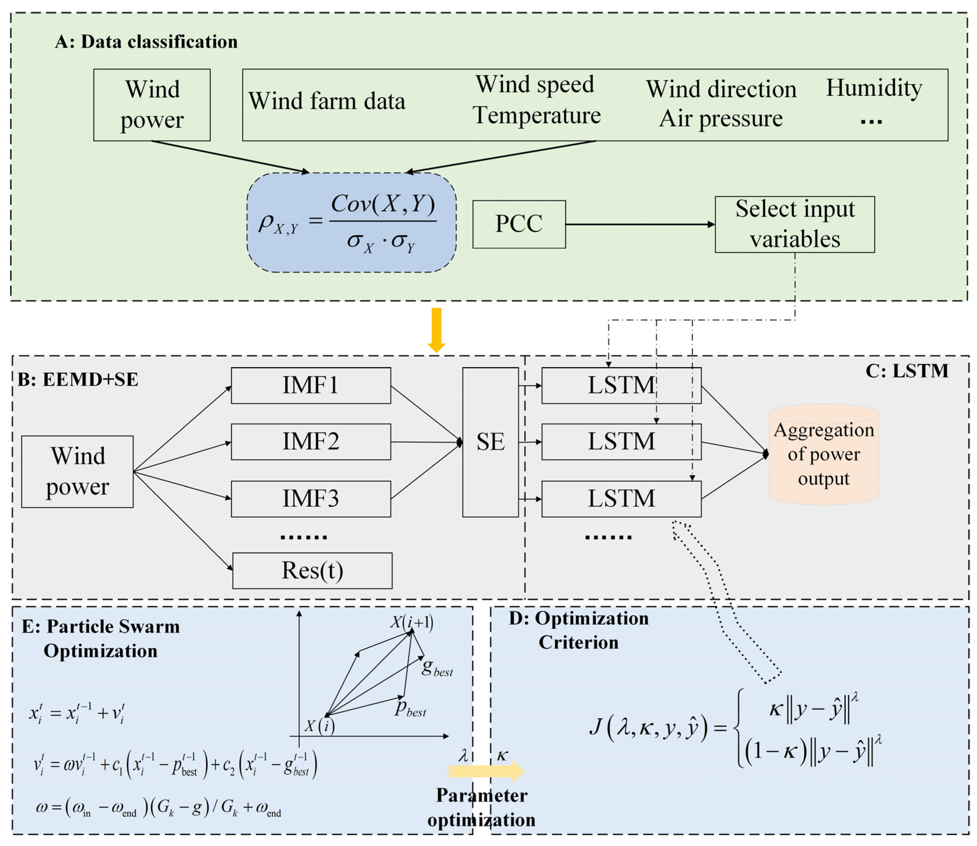
In this paper, according to the distribution of outliers in the wind farms, we derive the appropriate loss function, namely the ALF, for the inconsistency between the actual data and the MSE optimization criteria, which is expressed as follows:
J ( λ , κ , y , y ^ ) = { κ y y ^ p ,   y y ^ ( 1 κ ) y y ^ p , y y ^
where p and κ are the control coefficients, which are respectively determined as outliers; J ( p , κ , y , y ^ ) is the loss function; y and y ^ are the actual power and prediction, respectively.

2.5. Long Short-Term Memory

LSTM is a branch of the recurrent neural network (RNN), which can mine information at different time lengths. LSTM, originally created by Hochreiter and Schmidhuber, was further developed by Graves [25].
LSTM is specifically designed to avoid long-term dependency problems. In practice, LSTM’s mechanisms can handle long-term information, unlike the capabilities that other models acquire at great cost. The form of an RNN is a repetitive chain of neural network modules. The structure of the LSTM is shown in Figure 1.
The equation for LSTM is as follows:
f t = σ ( W f x t + U f h t 1 + b f ) i t = σ ( W i x t + U i h t 1 + b i ) c ˜ t = tanh ( W c x t + U c h t 1 + b c ) c t = f t c t 1 + i t c ˜ t h t = σ ( W o x t + U o h t 1 + b o ) tanh ( c t )
where f t is the forgetting gate; c ˜ is the input gate; x t is the current time input; h t 1 is the output state of the previous time; W and b are weighted and biased, respectively; σ and tanh are the sigmoid and tanh activation functions, respectively; is the number multiplication.
In this paper, LSTM is used to predict wind power. Moreover, it also addresses the problem of gradient disappearance and explosion.

2.6. Particle Swarm Optimization

In ALF, p and κ affect the function’s performance. Considering the simplicity of the model and the fewer parameters, PSO is adopted in this paper to optimize p and κ . PSO mimics the foraging behavior of birds in nature. Each individual in a flock is a massless “particle”, ignoring the mass and volume of each particle. Each particle has its own speed and position at the beginning of the iteration. The information interaction between the particles in the population is used to guide the particles in the whole population to converge to the optimal particles in the population while maintaining their own diversity information [11].
The individuals in PSO are called particles, and each particle swarm consists of N randomly initialized particles in the D-dimensional search space. In the search process, each particle i is represented by two vectors, namely, the velocity vector v i = [ v i 1 v i 2 v i D ] and the position vector x i = [ x i 1 x i 2 x i D ] . For each particle i , the speed and position of the individual historical best position and global best position update are used. The iterative equation is as follows:
v i t = ω v i t 1 + c 1 ( x i t 1 p best   t 1 ) + c 2 ( x i t 1 g b e s t t 1 )
ω = ( ω in   ω end   ) ( G k g ) / G k + ω end  
x i t = x i t 1 + v i t
where ω is the inertia weight; ω in   is the initial inertia value; ω end   is the maximum inertia value in the iteration; G k is the maximum number of iterations; c 1 and c 2 are the learning factors; v i t is the particle velocity in the t - t h iteration; g b e s t t 1 is the global optimal particle in the ( t 1 ) - t h iteration; p best   t 1 is the individual optimal particle in the ( t 1 ) - t h iteration; x i t is the particle position at the t - t h iteration.

2.7. Prediction Model

The designed prediction framework is shown in Figure 2. Considering the complexity of the meteorological data, PCC is proposed to extract the major meteorological data. Due to the non-stationary characteristics of wind power, EEMD is used to decompose the wind power sequences. Simultaneously, SE is used to analyze the correlation of the sub-modes. Considering the outliers in the data, a novel loss function is defined. Furthermore, the PSO is used to optimize the loss function. LSTM is then used to predict the power.

3. Discussion

In this section, the performance of the proposed prediction model is verified in three scenarios. All of the prediction models are based on a PC with an Intel (R) Core i5-9700 CPU @3.00 GHz and 8 GB RAM in MATLAB R2017b.

3.1. Data Description

Many studies have shown that there is a complex correlation between wind farm power and meteorological factors. Therefore, 13 sets of meteorological data are extracted from wind farms for analyses, including wind speed (at different heights), wind direction (at different heights), temperature, humidity, and air pressure. More detailed information is shown in Table 1. The time span of the data was from 1 January 2013 to 31 December 2013, with a data interval of 5 min.

3.2. Model Evaluation

In this paper, to quantify the overall performance of the model, the mean absolute error (MAE) and root mean square error (RMSE) are used [26,27] as follows:
M A E = 1 N i = 1 N ( y i y ^ i ) 2
R M S E = 1 N i = 1 N ( y i y ^ i ) 2

3.3. Discussion of PCC-ALF-LSTM and PSO-PCC-ALF-LSTM

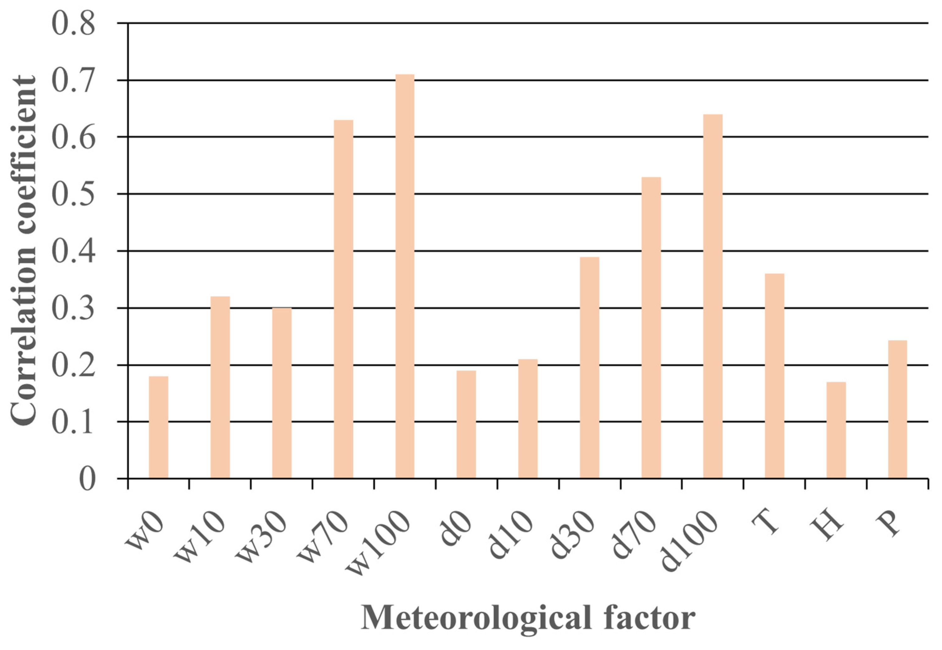
There are many meteorological factors that affect wind power. However, the influence of some of the data on the power can be ignored. Therefore, this paper adopts PCC for correlation analyses of the original meteorological data, which extracts the main meteorological data. In this paper, the threshold is set at 0.5. When the result of the meteorological factor is greater than 0.5, it is regarded as having a strong correlation, and the meteorological factor is selected as an input. Figure 3 shows the calculation results for the meteorological factors and the wind power. According to the threshold of the correlation coefficient, the relevant meteorological factors are selected, which are w70, w100, d70, and d100.
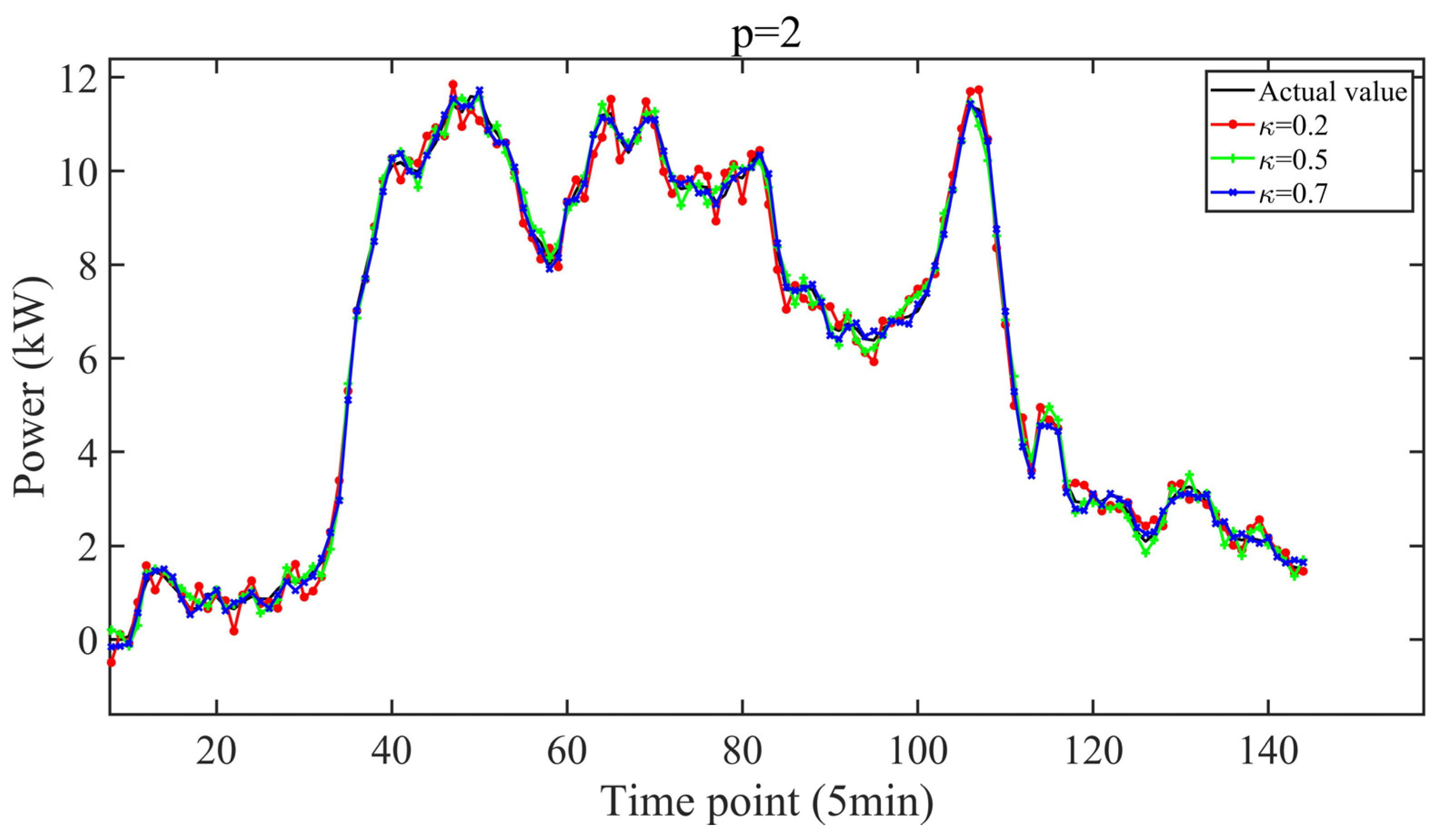
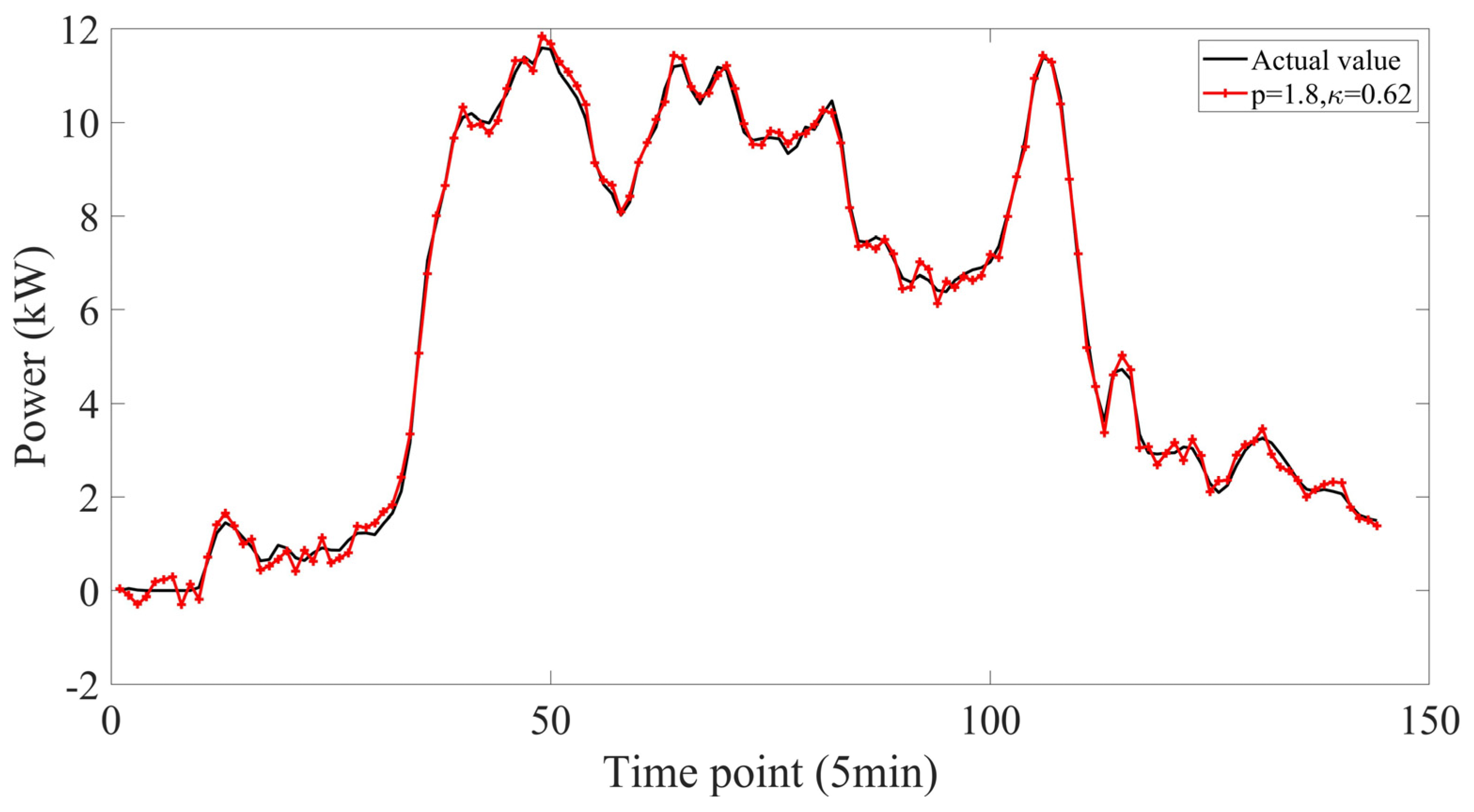
Data between June and August (summer) are selected to validate the proposed algorithm. The ratio of the training set to the test set is 7:3. Moreover, the 12-h forecast for the last day of the season is presented. The simulation of ALF with different parameters is shown in Figure 4 and Figure 5, where the ALF-LSTM effectively predicts the wind power. The prediction error is different for the different parameters. Therefore, PSO is introduced to optimize the parameters of ALF, which is described in detail in Section 2.6. The parameters of the PSO are set as follows: The particle population is 50. The inertia weight is between [0, 1]. c 1 = c 2 = 0.5 . The power prediction is shown in Figure 6. The MAE and RMSE for the different parameters are presented in Table 2. The following conclusions can be drawn: (a) the different parameters in ALF affect the prediction performance, where the different parameters of κ and p have different prediction errors caused by the outliers in the data; (b) when optimized by PSO, the error is effectively reduced.

3.4. Discussion of EEMD-SE-PSO-PCC-ALF-LSTM

In this section, EEMD-SE-PCC-ALF-LSTM is described and verified in detail.
Step 1. Data decomposition
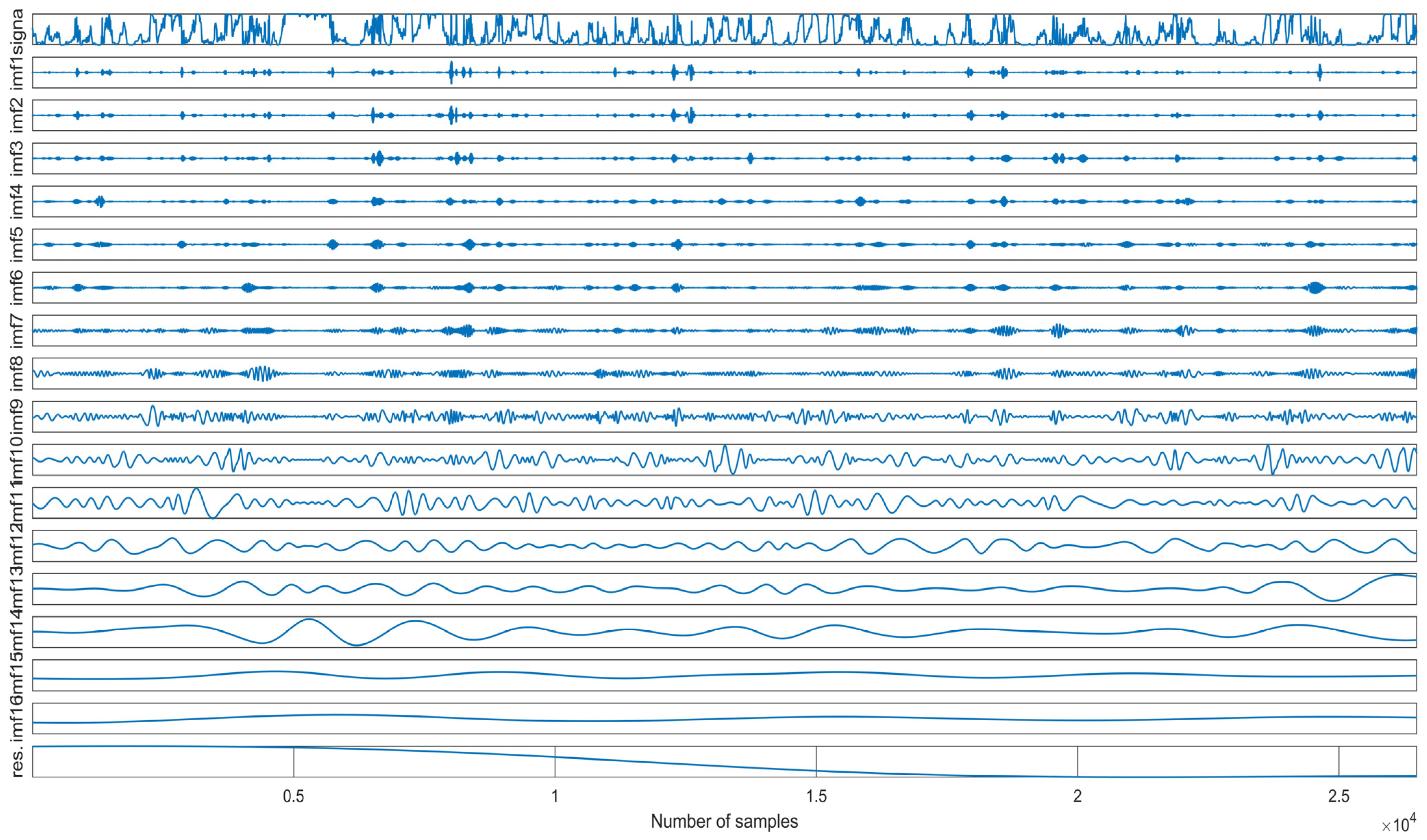
To solve the problem of wind power non-stationarity, EEMD is applied because of the characteristics of adaptive decomposition. The data decomposition results for the different sub-modes are shown in Figure 7, where the wind power is decomposed into 16 sub-modes.
Step 2. Sub-modes reconstructed by SE
With the power of EEMD decomposition, 16 sub-modes are determined. However, the 16 sub-modes are modeled separately, which increases the computing time of the model. Therefore, we use SE to measure the characteristics of the sub-modes to construct new feature sequences. A trial-and-error method is used to determine the appropriate parameters, as shown in Section 2.3. The reconstructed feature sequences are shown in Table 3. After SE, the 16 sub-modes are aggregated into three components, which reduces the complexity of the model.
Step 3. Component prediction
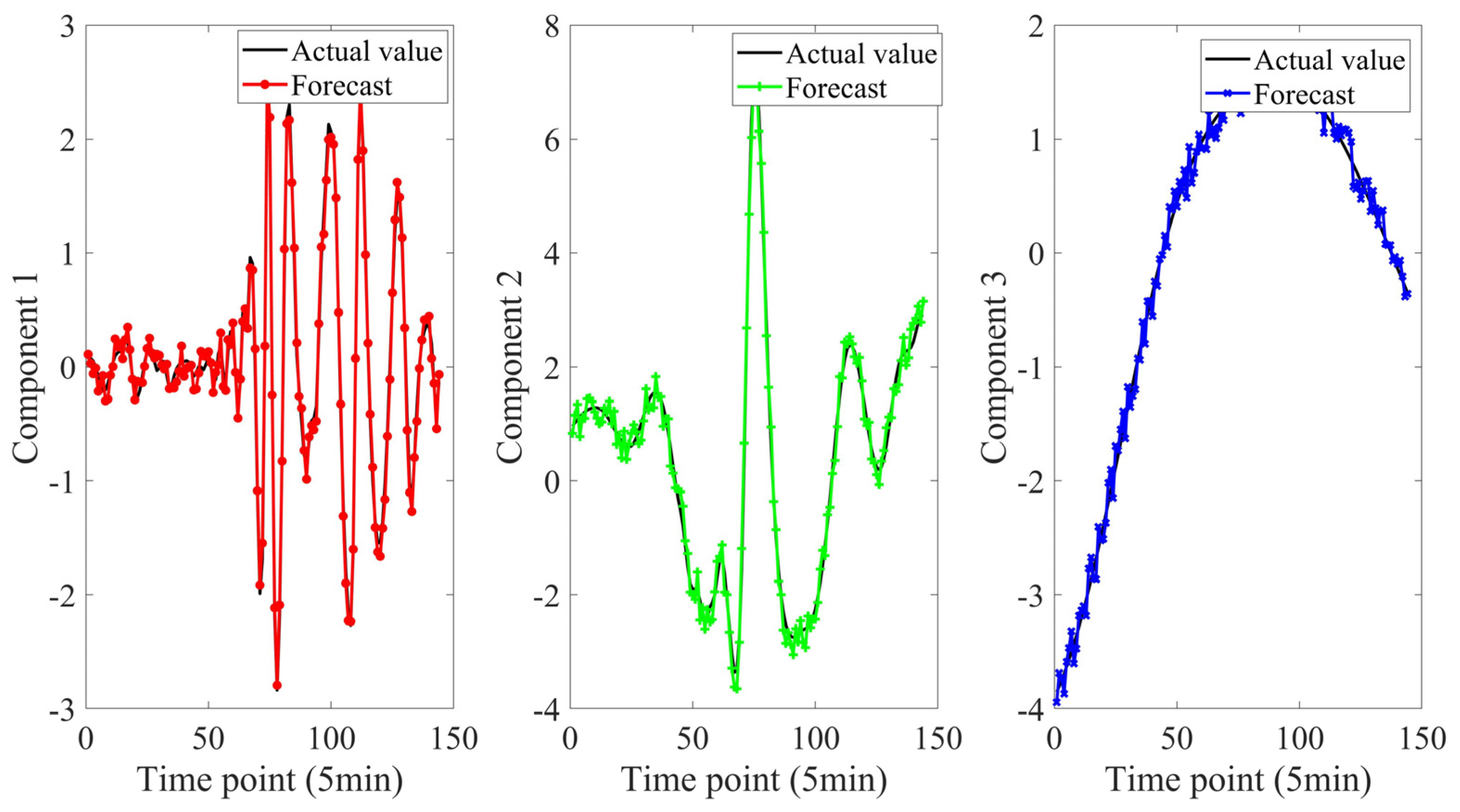
In this experiment, the ALF-LSTM model is used to predict each component. The residual is not considered in the reconfiguration. The input data are w70, w100, d70, and d100 in each component. The maximum epoch is 300, and the learning rate is 0.01. Additionally, the number of neurons is 32. The detailed parameters of the model are presented in Table 4. Meanwhile, the prediction models for each component are optimized by PSO. The predicted results are shown in Figure 8.
Step 4. Aggregation of predicted components
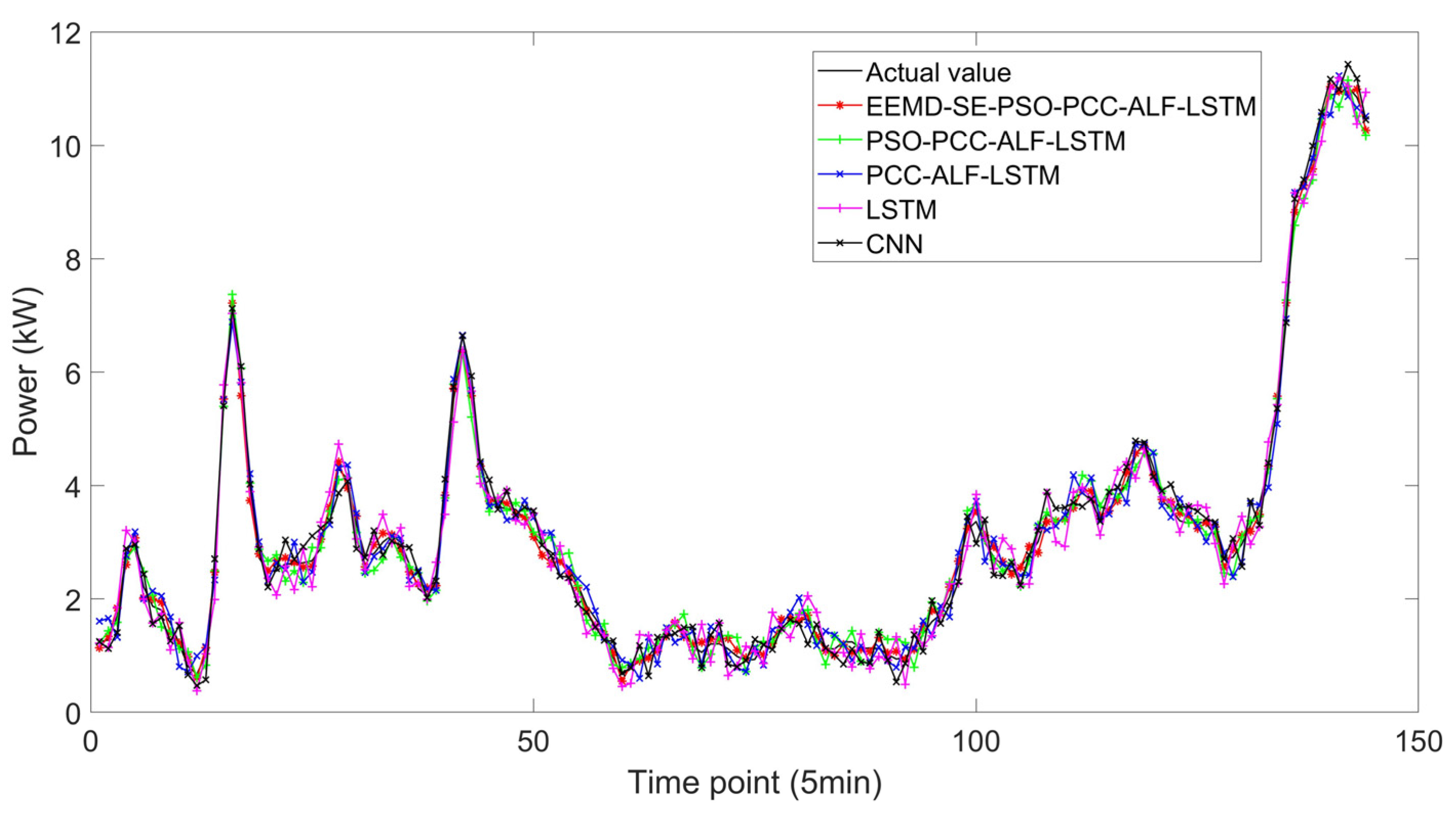
Finally, a linear aggregation of the components predicted by ALF-LSTM is carried out to obtain the prediction. The parameters of the model are shown in Table 3. Figure 9 shows the prediction results of EEMD-SE-PSO-PCC-ALF-LSTM, PSO-PCC-ALF-LSTM, and PCC-ALF-LSTM. The predictive performance of RMSE and MAE is evaluated, as shown in Table 5. The results show the following: (a) The proposed EEMD-SE-PSO-PCC-ALF-LSTM effectively reduces the wind power prediction error from 14.27 to 8.63 in RMSE; (b) The original power is decomposed and reconstructed by EEMD-SE, which reduces the fluctuation range, meaning that the method in this paper reduces the non-stationary characteristics of the power effectively by treating the power; (c) Although the hybrid prediction method constructed in this chapter needs to implement three PSO-PCC-ALF-LSTM prediction modules after processing the original power data, which increases the complexity of the model, this hybrid method can obtain a higher accuracy compared with other methods.

3.5. Discussion of the Comparison of Different Models

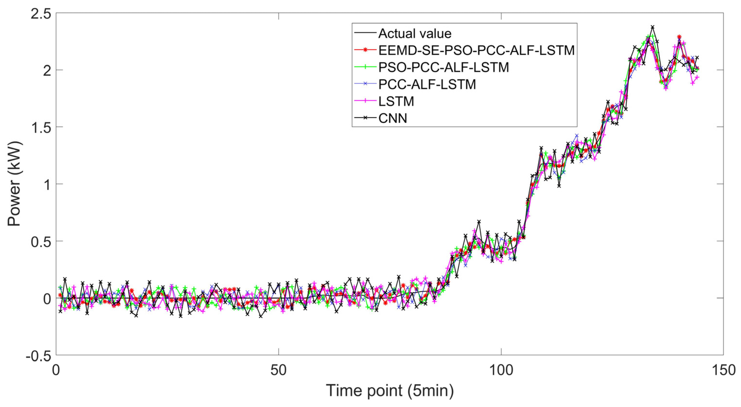
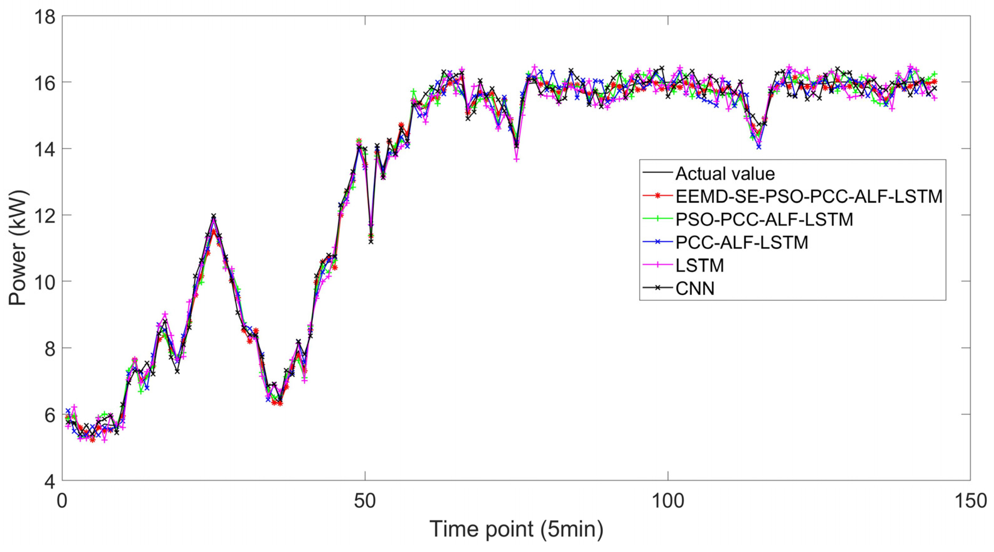
In this section, data from different seasons are analyzed. Meanwhile, LSTM is used as a comparison model in this paper, where the input data types are shown in Table 1. Similar to the prediction method in Section 3.4, the reconstructed components of the different seasons are shown in Table 6. The parameters of the model are shown in Table 7. It is worth noting that the parameters of PCC-ALF-LSTM, PSO-PCC-ALF-LSTM, LSTM (MSE), and the convolutional neural network (CNN) in Table 7 are shared with those in Table 8. The parameters of PCC-ALF-LSTM and PSO-PCC-ALF-LSTM are the same as those in Table 7. The forecast for the different seasons and forecast errors are shown in Table 9 and Figure 10, Figure 11 and Figure 12, respectively. The following conclusions are drawn: (a) In different seasons, the performance of LSTM (MSE) is the worst, and, on the contrary, other methods improve the accuracy; (b) The prediction performance of EEMD-SE-PSO-PCC-ALF-LSTM in the winter is poor, which accords with the objective law of winter weather variability; (c) Compared with LSTM (MSE) and CNN, the training time of the proposed model is longer, which is about 2 min in different seasons. However, since the shortest scheduling prediction time scale of the power system is 15 min, the proposed strategy meets the requirements.

4. Conclusions

Considering that wind farms are affected by weather, temperature, and random factors, PCC is proposed to extract the main influencing factors. Moreover, considering the large number of outliers in wind power, the optimization criterion of ALF-PSO is designed to ensure that the error distribution conforms to the real wind power bank data distribution. Furthermore, EEMD effectively deals with the non-stationarity of the power. SE is used to reconstruct the signal to reduce the complexity of the model. Finally, the effectiveness of EEMD-SE-PSO-PCC-ALF-LSTM is verified in different seasons. In the analysis, the power prediction error in the winter is larger than that in other seasons. Further work could consider different forecasting methods for specific seasons.

Author Contributions

Conceptualization, Y.D. and Q.S.; methodology, Y.D. and Q.S.; software, K.Z., Q.S. and Z.C.; validation, Y.D., K.Z. and Q.S.; formal analysis, Y.D.; investigation, Y.D. and K.Z.; resources, Y.D. and Q.S.; data curation, Y.D.; writing—original draft preparation, Y.D., K.Z., Q.S. and Z.C.; writing—review and editing, K.Z., Z.C., Q.S. and Y.D.; supervision, Q.S. All authors have read and agreed to the published version of the manuscript.

Funding

This research was funded by the National Key Research and Development Plan, grant number 2017YFB0902100.

Institutional Review Board Statement

Not applicable.

Informed Consent Statement

Not applicable.

Data Availability Statement

The datasets used and/or analyzed during the current study are available from the corresponding author upon reasonable request.

Acknowledgments

The authors gratefully acknowledge the support provided by the Shenyang University of Technology and the National Key Research and Development Plan.

Conflicts of Interest

The authors declare no conflict of interest.

References

  1. Bludszuweit, H.; Dominuez-Navarro, J.A.; Llombart, A. Statistical analysis of wind power forecast error. IEEE Trans. Power Syst. 2002, 23, 983–991. [Google Scholar] [CrossRef]
  2. Amjady, N.; Abedinia, O. Short term wind power prediction based on improved kriging interpolation, empirical mode decomposition, and closed-loop forecasting engine. Sustainability 2017, 9, 2104. [Google Scholar] [CrossRef] [Green Version]
  3. Landberg, L. A mathematical look at a physical power prediction model. Wind. Energy Inter-Natl. J. Prog. Appl. Wind. Power Convers. Technol. 1998, 1, 23–28. [Google Scholar] [CrossRef]
  4. Lange, M. Analysis of the Uncertainty of Wind Power Predictions; Universitat Oidenburg: Oldenburg, Germany, 2003. [Google Scholar]
  5. An, G.; Jiang, Z.; Chen, L.; Cao, X.; Li, Z.; Zhao, Y. Ultra short-term wind power forecasting based on sparrow search algorithm optimization deep extreme learning machine. Sustainability 2021, 13, 10453. [Google Scholar] [CrossRef]
  6. Liu, Y.; Wang, J. Transfer learning based multi-layer extreme learning machine for probabilistic wind power forecasting. Appl. Energy 2022, 312, 118729. [Google Scholar] [CrossRef]
  7. Zhang, C.; Hua, L.; Ji, C.; Shahzad Nazir, M.; Peng, T. An evolutionary robust solar radiation prediction model based on WT-CEEMDAN and IASO-optimized outlier robust extreme learning machine. Appl. Energy 2022, 32, 119518. [Google Scholar] [CrossRef]
  8. Liu, Z.; Mahdi, H.; Amirhosein, T. Novel forecasting model based on improved wavelet transform, informative feature selection, and hybrid support vector machine on wind power forecasting. J. Ambient. Intell. Humaniz. Comput. 2018, 9, 1919–1931. [Google Scholar] [CrossRef]
  9. Sun, W.; Wang, Y. Short-term wind speed forecasting based on fast ensemble empirical mode decomposition, phase space reconstruction, sample entropy and improved back-propagation neural network. Energy Convers. Manag. 2018, 157, 1–12. [Google Scholar] [CrossRef]
  10. Zhang, S.H. Wind power prediction based on genetic neural network. AIP Conf. Proc. 2017, 1834, 020012. [Google Scholar]
  11. Ma, T.; Wang, C.; Wang, J. Particle-swarm optimization of ensemble neural networks with negative correlation learning for forecasting short-term wind speed of wind farms in western China. Inf. Sci. 2019, 505, 157–182. [Google Scholar] [CrossRef]
  12. Eltamaly, A.M.; Farh, H.; Saud, M. Impact of PSO reinitialization on the accuracy of dynamic global maximum power detection of variant partially shaded PV systems. Sustainability 2019, 11, 2091. [Google Scholar] [CrossRef] [Green Version]
  13. Wu, Q.; Lin, H. Short-term wind speed forecasting based on hybrid variational mode decomposition and least squares support vector machine optimized by bat algorithm model. Sustainability 2019, 11, 652. [Google Scholar] [CrossRef] [Green Version]
  14. Liao, C.W.; Wang, I.; Lin, K.P. A fuzzy seasonal long short-term memory network for wind power forecasting. Mathematics 2021, 9, 1178. [Google Scholar] [CrossRef]
  15. Zheng, W.; Bo, W.; Liu, C. Improved BP neural network algorithm to wind power forecast. J. Eng. 2017, 13, 940–943. [Google Scholar]
  16. Jiang, Y.; Zhang, B.; Xing, F. Super-short-term multi-step prediction of wind power based on GA-VNN model of chaotic time series. Power Syst. Technol. 2015, 39, 2160–2166. [Google Scholar]
  17. Bourakadi, D.E.; Yahyaouy, A.; Boumhidi, J. Improved extreme learning machine with autoencoder and particle swarm optimization for short-term wind power prediction. Neural Comput. Appl. 2021, 34, 4643–4659. [Google Scholar] [CrossRef]
  18. Zhou, B.; Ma, X.; Luo, Y. Wind power prediction based on LSTM networks and nonparametric kernel density estimation. IEEE Access 2019, 7, 165279–165292. [Google Scholar] [CrossRef]
  19. Wang, Y.; Shen, R.; Ma, Y.; Ma, M.; Zhou, Q.; Lu, Q.; Zhang, J. Research on ultra-short term forecasting technology of wind power output based on wake model. J. Phys. Conf. Ser. 2022, 2166, 012041. [Google Scholar] [CrossRef]
  20. Jaihuni, M.; Basak, J.K.; Khan, F.; Okyere, F.G.; Sihalath, T.; Bhujel, A.; Park, J.; Lee, D.H.; Kim, H.T. A novel recurrent neural network approach in forecasting short term solar irradiance. ISA Trans. 2022, 121, 63–74. [Google Scholar] [CrossRef]
  21. Wang, W.; Tian, G.; Yuan, G.; Pham, D.T. Energy-time tradeoffs for remanufacturing system scheduling using an invasive weed optimization algorithm. J. Intell. Manuf. 2021, 34, 1065–1083. [Google Scholar] [CrossRef]
  22. Lu, P.; Ye, L.; Pei, M. Short-term wind power forecasting based on meteorological feature extraction and optimization strategy. Renew. Energy 2022, 184, 198–216. [Google Scholar] [CrossRef]
  23. Yin, H.; Ou, Z.; Huang, S.; Meng, A. A cascaded deep learning wind power prediction approach based on a two-layer of mode decomposition. Energy 2019, 189, 301–316. [Google Scholar] [CrossRef]
  24. Richman, J.S.; Moorman, J.R. Physiological time-series analysis using approximate entropy and sample entropy. Am. J. Physiol. Heart Circ. Physiol. 2000, 278, H2039–H2049. [Google Scholar] [CrossRef] [PubMed] [Green Version]
  25. Ahmad, T.; Zhang, D. A data-driven deep sequence-to-sequence long-short memory method along with a gated recurrent neural network for wind power forecasting. Energy 2022, 239, 369–397. [Google Scholar] [CrossRef]
  26. Song, Z.; Jiang, Y.; Zhang, Z. Short-term wind speed forecasting with markov-switching model. Appl. Energy 2014, 130, 103–112. [Google Scholar] [CrossRef]
  27. Li, G.; Shi, J. On comparing three artificial neural networks for wind speed forecasting. Appl. Energy 2010, 87, 2313–2320. [Google Scholar] [CrossRef]
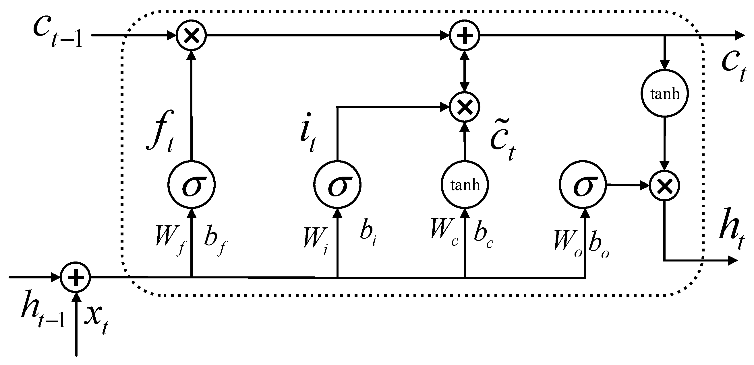
Figure 1. The structure of LSTM.
Sustainability 15 06285 g001
Figure 2. The framework of the proposed model.
Sustainability 15 06285 g002
Figure 3. Correlation analysis.
Sustainability 15 06285 g003
Figure 4. Wind power for the different κ parameters.
Sustainability 15 06285 g004
Figure 5. Wind power for the different P parameters.
Sustainability 15 06285 g005
Figure 6. Wind power for the parameters optimized by PSO.
Sustainability 15 06285 g006
Figure 7. Sub-modes decomposed by EEMD.
Sustainability 15 06285 g007
Figure 8. The prediction of each component.
Sustainability 15 06285 g008
Figure 9. The results predicted by the proposed algorithm (summer).
Sustainability 15 06285 g009
Figure 10. Power prediction (spring).
Sustainability 15 06285 g010
Figure 11. Power prediction (autumn).
Sustainability 15 06285 g011
Figure 12. Power prediction (winter).
Sustainability 15 06285 g012
Table 1. Meteorological data.
Meteorological FactorAbbreviationUnit
wind speed at 0 m
wind speed at 10 mw10m/s
wind speed at 30 mw30m/s
wind speed at 70 mw70m/s
wind speed at 100 mw100m/s
wind direction at 0 m
wind direction at 10 md10°
wind direction at 30 md30°
wind direction at 70 md70°
wind direction at 100 md100°
temperatureT
humidityH%rh
pressurePPa
Table 2. MAE and RMSE of different parameters (summer).
ParametersMAERMSE
p = 2 κ = 0.2 8.1311.31
κ = 0.5 9.6712.18
κ = 0.7 8.0711.24
κ = 0.5 p = 1.5 7.6210.36
p = 2 9.6712.18
p = 2.5 8.6911.74
PSO optimization
p = 1.53 ,   κ = 0.63
7.519.36
Table 3. Analysis of the components by SE.
Reconstruction ComponentSub-Model
Component 1IMF1, IMF5, IMF7, IMF12-15
Component 2IMF2, IMF10, IMF11, IMF12-16
Component 3IMF3, IMF4, IMF6, IMF8, IMF9
Table 4. Parameters of the model.
ModelParameters
ALFPSOSELSTM
PCC-ALF-LSTM p = 2 , κ = 0.2 //Maximum epoch: 300.
Learning rate: 0.01.
Number of neurons: 32
PSO-PCC-ALF-LSTM p = 2 , κ = 0.2 Population :   50 .   Inertia   weight :   [ 0 ,   1 ] .   c 1 = c 2 = 0.5 /
EEMD-SE-PSO-PCC-ALF-LSTM Component   1 :   p = 1.73 , κ = 0.42 m = 2 ,   r = 0.25 s t d
Component   2 :   p = 1.68 , κ = 0.53
Component   3 :   p = 1.97 , κ = 0.59
std is the standard deviation of the decomposition sub-model.
Table 5. MAE and RMSE of different models (summer).
ModelMAERMSE
PCC-ALF-LSTM8.3414.27
PSO-PCC-ALF-LSTM7.369.91
EEMD-SE-PSO-PCC-ALF-LSTM6.788.63
Table 6. The reconstructed components of SE in different seasons.
SeasonReconstruction ComponentSub-Model
SpringComponent 1IMF1, IMF5, IMF7, IMF12-15
Component 2IMF2, IMF10, IMF11, IMF12-14
Component 3IMF3, IMF6, IMF8, IMF9
Component 4IMF4, IMF15-17
AutumnComponent 1IMF1, IMF6, IMF10, IMF13
Component 2IMF2, IMF7, IMF9, IMF14
Component 3IMF3, IMF8, IMF11
Component 4IMF4, IMF5, IMF9, IMF15-17
WinterComponent 1IMF1, IMF7, IMF9, IMF11
Component 2IMF2, IMF4, IMF10, IMF12
Component 3IMF3, IMF5, IMF6, IMF13-14
Table 7. Parameters of the model (spring).
ModelParameters
ALFPSOSELSTM
PCC-ALF-LSTM p = 2 , κ = 0.2 //Maximum epoch: 300.
Learning rate: 0.01.
Number of neurons: 32. Hidden layer: 3.
/
PSO-PCC-ALF-LSTM p = 2 , κ = 0.2 Population :   50 .   Inertia   weight :   [ 0 ,   1 ] .   c 1 = c 2 = 0.5 //
EEMD-SE-PSO-PCC-ALF-LSTM Component   1 :   p = 2.13 , κ = 0.41 m = 1.6 ,   r = 0.25 s t d /
Component   2 :   p = 2.07 , κ = 0.57
Component   3 :   p = 1.82 , κ = 0.47
Component   4 :   p = 1.94 , κ = 0.39
LSTM (MSE)////
CNNConvolutional layers: 5, Kernel number: 5, Kernel size: 2 * 2, Number of full connection layers: 8, Output layer: 1
Table 8. Parameters of the model (autumn, winter).
ModelEEMD-SE-PSO-PCC-ALF-LSTM
SeasonAutumnWinter
Parameters Component   1 :   p = 2.09 , κ = 0.56 Component   2 :   p = 1.84 , κ = 0.53 Component   3 :   p = 1.96 , κ = 0.42 Component   4 :   p = 2.01 , κ = 0.49 Component   1 :   p = 1.72 , κ = 0.56 Component   2 :   p = 1.87 , κ = 0.61 Component   3 :   p = 1.97 , κ = 0.53
Table 9. MAE and RMSE (spring, autumn, winter).
SeasonModelMAERMSETraining Time (s)
SpringPCC-ALF-LSTM9.6313.6946.78
PSO-PCC-ALF-LSTM7.9710.3257.59
EEMD-SE-PSO-PCC-ALF-LSTM6.329.12103.37
LSTM9.5712.9745.37
CNN9.3611.7739.87
AutumnPCC-ALF-LSTM8.4711.3645.97
PSO-PCC-ALF-LSTM7.489.5759.34
EEMD-SE-PSO-PCC-ALF-LSTM7.068.32112.01
LSTM9.1212.3543.62
CNN8.9711.8937.39
WinterPCC-ALF-LSTM11.3614.3648.35
PSO-PCC-ALF-LSTM10.5813.8555.19
EEMD-SE-PSO-PCC-ALF-LSTM8.9612.31117.38
LSTM13.7415.9746.37
CNN12.3514.8640.43
Disclaimer/Publisher’s Note: The statements, opinions and data contained in all publications are solely those of the individual author(s) and contributor(s) and not of MDPI and/or the editor(s). MDPI and/or the editor(s) disclaim responsibility for any injury to people or property resulting from any ideas, methods, instructions or products referred to in the content.