Article

Forecasting and Uncertainty Analysis of Day-Ahead Photovoltaic Power Based on WT-CNN-BiLSTM-AM-GMM

1
School of Electrical Engineering, North China University of Water Resources and Electric Power, Zhengzhou 450011, China
2
Xinyang Power Supply Company of State Grid Henan Electric Power Company, Xinyang 464000, China
3
Henan Jiuyu Tenglong Information Engineering Co., Ltd., Zhengzhou 450052, China
*
Author to whom correspondence should be addressed.
Sustainability 2023, 15(8), 6538; https://doi.org/10.3390/su15086538
Submission received: 23 February 2023 / Revised: 16 March 2023 / Accepted: 17 March 2023 / Published: 12 April 2023

Abstract

:
Accurate forecasting of photovoltaic (PV) power is of great significance for the safe, stable, and economical operation of power grids. Therefore, a day-ahead photovoltaic power forecasting (PPF) and uncertainty analysis method based on WT-CNN-BiLSTM-AM-GMM is proposed in this paper. Wavelet transform (WT) is used to decompose numerical weather prediction (NWP) data and photovoltaic power data into frequency data with time information, which eliminates the influence of randomness and volatility in the data information on the forecasting accuracy. A convolutional neural network (CNN) is used to deeply mine the seasonal characteristics of the input data and the correlation characteristics between the input data. The bidirectional long short-term memory network (BiLSTM) is used to deeply explore the temporal correlation of the input data series. To reflect the different influences of the input data sequence on the model forecasting accuracy, the weight of the calculated value of the BiLSTM model for each input data is adaptively adjusted using the attention mechanism (AM) algorithm according to the data sequence, which further improves the model forecasting accuracy. To accurately calculate the probability density distribution characteristics of photovoltaic forecasting errors, the Gaussian mixture model (GMM) method was used to calculate the probability density distribution of forecasting errors, and the confidence interval of the day-ahead PPF was calculated. Using a photovoltaic power station as the calculation object, the forecasting results of the WT-CNN-BiLSTM-AM, CNN-BiLSTM, WT-CNN-BiLSTM, long short-term memory network (LSTM), gate recurrent unit (GRU), and PSO-BP models were compared and analyzed. The calculation results show that the forecasting accuracy of the WT-CNN-BiLSTM-AM model is higher than that of the other models. The confidence interval coverage calculated from the GMM is greater than the given confidence level.

1. Introduction

Solar energy, as an important energy source for solving the rapid increase in energy demand and depletion of fossil fuels, has been developed and utilized on a large scale in recent years. According to the “Renewable Energy Statistics 2021” released by the International Renewable Energy Agency (IRENA), in 2020, the new global photovoltaic installed capacity was 127 GW, and the total installed capacity reached 760.4 GW [1]. The photovoltaic power generation process is affected by environmental factors such as light intensity, wind speed and direction, temperature, and humidity, which makes it highly random, volatile, and uncertain. These characteristics pose great challenges to the safe and stable operation of power grids [2,3]. Therefore, accurate forecasting of photovoltaic power is the key way to ensure the safe and stable operation of the power grid, reasonably arrange energy scheduling, and improve photovoltaic power consumption [4].
According to the different time scales of photovoltaic power forecasting (PPF), PPF can be divided into three forecasting time scales: medium- and long-term forecasts, short-term forecasts, and ultra-short-term forecasts [5,6,7]. According to the different forecasting mechanisms, the PPF can be divided into physical, statistical, machine learning, and deep learning forecasting methods [8,9,10]. The physical forecasting method involves building a photovoltaic power generation model according to the conversion mechanism of photovoltaic cells, and then calculating the output power of the photovoltaic power station according to numerical weather prediction (NWP) data [11,12]. The parameter value of the actual photovoltaic power generation system gradually changes with an increase in running time, which gradually reduces the forecasting accuracy of the physical forecasting model [13].
Statistical forecasting methods use statistical models to describe the mapping relationship between the output power of the photovoltaic power station and the input variables (including the NWP dataset and measurement dataset of the photovoltaic power station) [14]. Common statistical forecasting methods include the autoregressive integrated moving average (ARIMA) [15], autoregressive and moving average (ARMA) [16], and regression analysis [17]. Statistical forecasting methods have good forecasting accuracy for ultra-short-term PPF; however, with an increase in forecasting time, the forecasting accuracy of the statistical model decreases, and the statistical model cannot accurately describe the nonlinear characteristics between the input data and the output power, which further limits the wide use of statistical forecasting methods [10].
Machine learning can extract complex nonlinear features from high-dimensional data, which supports the construction of high-precision PPF models based on machine learning [18,19]. Gu et al. [20] used the advantages of fast convergence speed and high convergence accuracy of the whale optimization algorithm (WOA) to optimize the penalty factor and kernel function width of the least squares support vector machine (LSSVM) model, which effectively improved its calculation speed and forecasting accuracy of the LSSVM model. The calculation results show that the forecasting accuracy of the WOA-LSSVM model was higher than that of the original LSSVM model. Wang et al. [21] compared the short-term PPF accuracy of the LASSO regression, random forest regression, gradient propulsion regression, and support vector regression models, and the computational results showed that the forecasting accuracy of the support vector regression model was higher than that of the other models. A PPF system was constructed by combining the variational mode decomposition strategy based on a genetic algorithm and multi-objective grasshopper optimization algorithm, and the PPF system can accurately forecast the output power of the photovoltaic power station in the next 1 h [22]. The machine learning and spatiotemporal parameter optimization algorithms were combined to forecast the photovoltaic power in the next 10 min. The forecasting results showed that the forecasting accuracy of this method was higher than that of the benchmark model [23].
Neural network models, such as machine learning models with powerful nonlinear mapping capabilities, have been extensively researched and applied in the analysis of photovoltaic plant operation status and power forecasting [24,25]. Natarajan et al. [26] used a radial belief neural network (RBNN) to forecast the output power of photovoltaic power stations with different capacities. The calculation results showed that the RBNN model can achieve good forecasting accuracy. Moreira et al. [27] combined an experimental method with an artificial neural network model to forecast the photovoltaic power output in the following week. The calculation results showed that the weekly average absolute percentage error of the forecasting results of this model was 4.7%, with high forecasting accuracy. Hassan et al. [7] proposed a nonlinear autoregressive neural network model optimized through a genetic algorithm and applied the model to forecast the output power of photovoltaic power stations at five different locations in Algeria and Australia. The calculation results showed that the model had a good forecasting effect and adaptability. Ma et al. [28] established a short-term PPF model based on an Elman neural network optimized using a modified firefly algorithm, which effectively solved the problems of randomness of the initial weights and thresholds of the basic Elman neural network, the slow training speed, and effectively improved the forecasting accuracy of the Elman neural network.
Although neural networks have strong nonlinear mapping capabilities, they do not have the ability to extract the temporal correlation features and deep features of data, which limits the improvement of the forecasting accuracy of neural network models [8,9]. With the development of artificial intelligence technology, deep learning algorithms have shown extraordinary capabilities in nonlinear mapping, data temporal correlation features, and deep feature extraction, which have been intensively studied and applied in short-term PPF in recent years [29,30,31]. Garazi et al. [32] compared and analyzed the forecasting accuracy of long short-term memory networks (LSTM) and convolutional neural networks (CNN) in 1-h ahead PPF, and the computational results showed that the forecasting accuracy of CNN was better than that of LSTM. Mellit et al. [33] tested the short-term PPF performance of deep neural network models, such as LSTM, BiLSTM, gated recurrent unit (GRU), bi-directional GRU (BiGRU), and CNN. Zang et al. [34] used deep convolutional neural networks (DCNs) to forecast day-ahead photovoltaic power, and their computational results showed that DCNs have good forecasting accuracy.
Combining the advantages of several deep learning algorithms to build PPF models can effectively improve the model’s forecasting accuracy [35,36]. Yang et al. [37,38] combined the attention mechanism (AM), CNN, and BiLSTM to build a day-ahead PPF model. The calculation results showed that the forecasting accuracy of this hybrid model was higher than that of other models. Khan et al. [39] proposed a hybrid PPF model based on a stack-integration algorithm and LSTM. Through a comparison with single ANN, LSTM, and bagging models, the results show that the forecasting accuracy of the proposed hybrid model was higher than that of the single model. Akhter et al. [40,41] proposed a PPF model based on the hybrid salp swarm algorithm, recurrent neural network, and LSMT, and applied the hybrid model for PPF 1-h ahead. The calculation results showed that the forecasting accuracy of the hybrid model was higher than that of the RNN-LSTM, GA-RNN-LSTM, and PSO-RNN-LSTM models.
Accurately calculating the uncertainty of the PPF can further reduce the adverse impact of photovoltaic power change on the stable operation of the power system [42]. The uncertainty of the PPF is mostly described using confidence intervals, which can be calculated through parametric methods, nonparametric methods, and uncertainty factor decomposition and superposition [14]. Parametric methods assume that the single-point forecasting error band at future moments is a fixed historical empirical value or that the error distribution obeys a particular form of distribution [43]. Commonly used parametric methods include probabilistic statistical models [44], Bayesian models [45], and copula models [46]. However, the PPF error does not obey any known distribution function, and the calculation accuracy of various fitting functions varies significantly in different scenarios and periods. These factors limit the application of parametric methods [47].
The nonparametric method directly calculates the distribution characteristics of the forecasting error according to the error value of PPF, without assuming the distribution form of the forecasting error value, which helps to improve the accurate description of the distribution characteristics of forecasting. Commonly used nonparametric methods include quantile regression [48], Monte Carlo [49], and sample entropy [50]. The calculation methods for uncertainty factor decomposition and superposition consider all factors that may lead to forecasting uncertainty, including data noise [51], NWP error [52], and actual power curve dispersion [53]. Although the uncertainty factor decomposition and superposition methods can accurately calculate the confidence interval range, their implementation process is complex, and the calculation time is long.
Based on the current research status of PPF, this study proposes a day-ahead PPF and uncertainty analysis method that combines the wavelet transform (WT), convolutional neural network (CNN), bidirectional long short-term memory network (BiLSTM), attention mechanism (AM), and Gaussian mixture model (GMM). This method uses WT to decompose NWP data and photovoltaic power data into frequency data with time information, thereby eliminating the influence of randomness and volatility in NWP data and photovoltaic power data on forecasting accuracy. Combining the model advantages of CNN, BiLSTM, and AM, the WT-CNN-BiLSTM-AM forecasting model is constructed to realize the deep mining of the seasonal characteristics of data, the correlation characteristics between data, and the temporal correlation of the data series, and effectively improve the forecasting accuracy of the hybrid model. To accurately calculate the probability density distribution characteristics of the PPF error, GMM was used to calculate the probability density distribution of forecasting errors, and the confidence interval of the PPF for day-ahead was calculated.
The remainder of this paper is organized as follows: Section 2 elaborates on the principle of the WT algorithm and the WT decomposition process of NWP data and photovoltaic power data. The construction process of the CNN-BiLSTM-AM model is described in Section 3. The modeling process of the GMM and confidence interval is described in Section 4. Section 5 analyzes the data source and the relationship between the size of the training dataset and forecasting accuracy of the model in detail. The forecasting accuracy of the different forecasting models is calculated and analyzed in Section 6. The probability density estimation of the PPF errors and the calculation method for the confidence interval are described in Section 7. Finally, Section 8 concludes the study.

2. Wavelet Transform of Data

The NWP data and photovoltaic power data have strong randomness and volatility, and the existing PPF models cannot accurately mine the randomness and volatility of data, which is one of the main factors affecting the forecasting accuracy of PPF. The randomness and volatility of the NWP data and photovoltaic power data are mainly reflected in the high-frequency components in the frequency domain. Therefore, this study uses wavelet transform (WT) to decompose NWP data and photovoltaic power data into data information of different frequencies, inputs the decomposed frequency data into the forecasting model for calculation, and fuses the calculation results of the forecasting model to obtain the final forecasting result. In this section, the WT process of the NWP data and photovoltaic power data is described in detail.
WT evolved from the Fourier transform. In WT, the basis function of the Fourier transform is transformed into a wavelet basis. This transformation realizes the extraction of time domain information and frequency domain information of time-series data and effectively enhances the data representation ability [54]. The WT converts NWP data and photovoltaic power data into time series data of different frequencies, which not only preserves the time correlation characteristics between the data but also converts the randomness and volatility of the original data into time series data of high-frequency components. These time series data of high-frequency components, as part of the input data of the forecasting model, realize the deep mining of the randomness and volatility of the original data and further improve the forecasting accuracy of the forecasting model.
Figure 1 shows the data series after WT of photovoltaic power data, where the original photovoltaic power data are collected in the frequency range of 0–120 Hz: A1 denotes the data series with a wavelet transformed frequency of 0–4 Hz; A2 denotes the data series with a wavelet transformed frequency of 4–8 Hz; A3 denotes the data series with a wavelet transformed frequency of 8–16 Hz; A4 denotes the data series with a wavelet transformed frequency of 16–32 Hz; and A5 represents the data sequence with a frequency of 32–64 Hz after wavelet transformation. As shown in Figure 1, the low-frequency series of data (shown as A1 in Figure 1) reflects the overall trend of the original photovoltaic power data, whereas the high-frequency part of the data (A2, A3, A4, and A5 in Figure 1) describes the randomness and volatility of the data in detail. Therefore, the NWP data and photovoltaic power data are converted into time series data of different frequencies, and the converted data series of different frequencies are used as the training dataset and test dataset of the forecasting model, which not only retains the time correlation characteristics between the data, but also realizes the deep mining of the randomness and volatility of the original data, which can further improve the forecasting accuracy of the forecasting model.

3. CNN-BiLSTM-AM Forecasting Model

3.1. Principle of Convolutional Neural Network

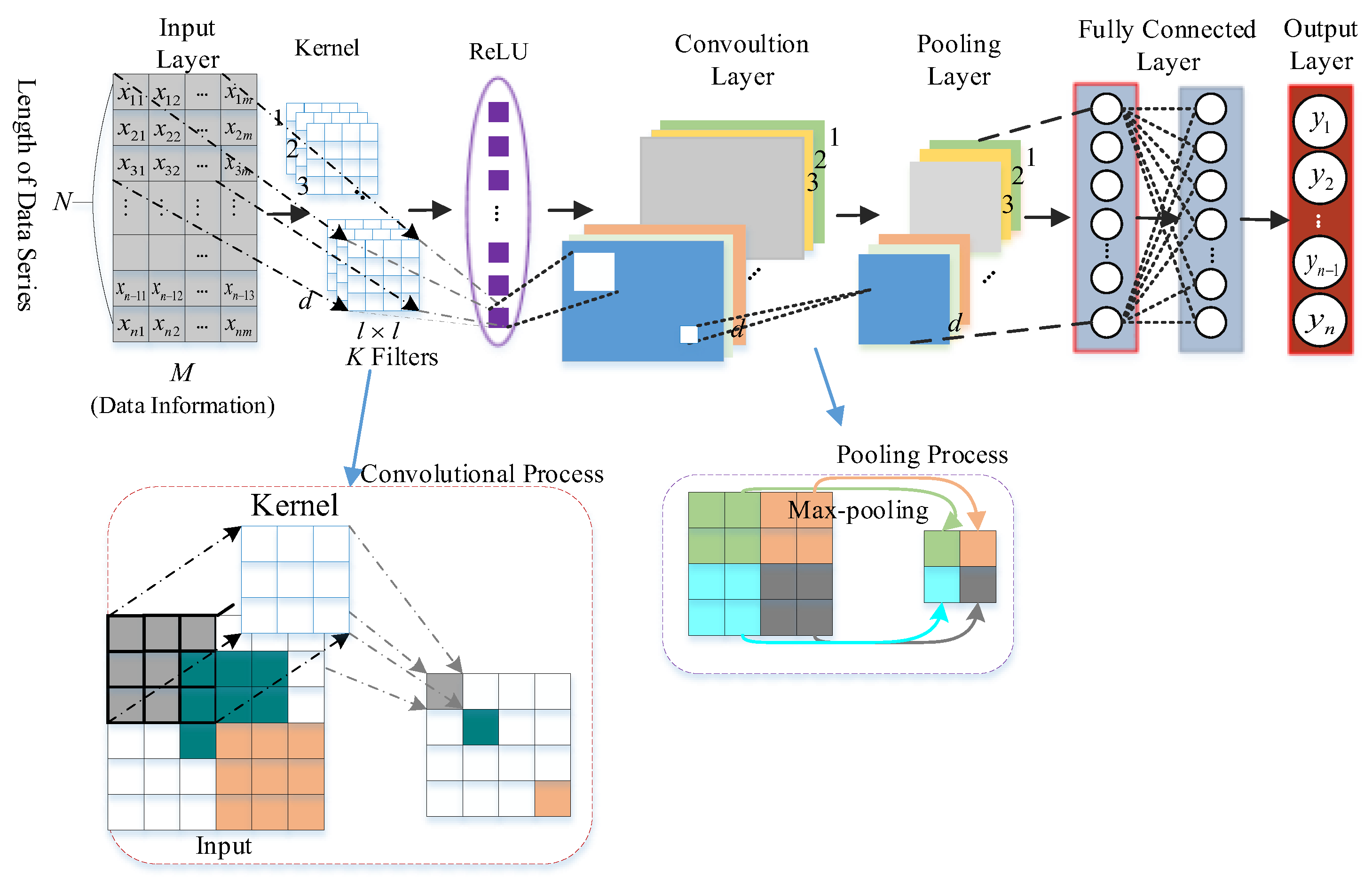
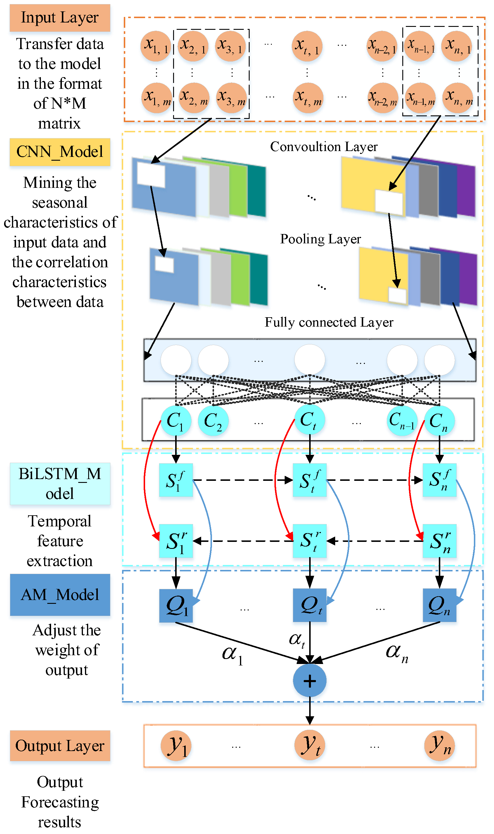
Convolutional neural networks (CNN) effectively reduce the number of parameters and data dimensions of deep neural networks while deeply mining the spatial characteristics of input data through local connectivity, weight sharing, and pooling operations, which effectively improves the computational speed and data analysis capability of CNN. The basic structure of the CNN consists of an input layer, a convolutional layer, a pooling layer, a fully connected layer, and an output layer, as shown in Figure 2.
(1)
Input Layer
The input layer is mainly used to obtain the input data of the CNN. In this study, the input data are photovoltaic power data and NWP data, and when the unit-scale of the input data is inconsistent, it will seriously affect the forecasting accuracy of the model. To eliminate the impact of unit-scale inconsistency on the forecasting accuracy of the model, it is necessary to normalize the data before they are transferred to the input layer. In this study, the photovoltaic power data and NWP data were normalized to the range of [0, 1]. The input data are a data matrix of N*M, where N is the length of the time series of data, and M is the data information of power, wind speed, wind direction, temperature, and humidity at each moment point. The structure of the time series data is shown in Figure 2.
(2)
Convolutional Layer
The convolution layer is the core component of the CNN, which extracts the spatial distribution features of the input data using a convolution operation. To extract the seasonal characteristics and correlation characteristics between data from photovoltaic power data and NWP data, this study uses 50 convolution kernels to convolute the input data. The convolution calculation formula is given by Equations (1) and (2), respectively.
c i ,   j d = f x i , j , , x i ,   j + l 1 , , x i ,   j + l 1 ,   j , , x i + l 1 ,   j + l 1 K d + b d
C d = c 1 ,   1 d ,   c 1 ,   2 d ,   , c 1 ,   M l + 1 d c 2 ,   1 d ,   c 2 ,   2 d ,   , c 2 ,   M l + 1 d                     ,   , c N l + 1 ,   1 d   ,   , c N l + 1 ,   M l + 1 d
In the above Equations (1) and (2), K d is the d-th convolution kernel, the matrix of the convolution kernel size is l × l , f is the activation function of the neurons, b d is the threshold of the d-th activation function, and c i ,   j d is the output of the i row and j column neurons calculated by the d-th convolution kernel.
The linear rectification function is computationally simple and can effectively overcome the gradient vanishing problem of activation functions such as tanh and logistic functions. Therefore, a rectified linear unit (ReLU) is used as the activation function of the neuron in the convolution calculation. The linear rectification function is given by Equation (3).
f ( x ) = R e L U ( x ) = m a x ( 0 ,   1 )
The computation process of the convolutional layer is shown in the convolutional layer in Figure 2.
(3)
Pooling Layer
The pooling layer was used to reduce the dimensionality of the input high-dimensional feature data, improve the computational speed of the CNN, and prevent overfitting. Common pooling calculation methods include max-pooling, mean-pooling, and stochastic pooling. According to the distribution characteristics of photovoltaic power data and NWP data, the maximum pooling method was selected for the calculation. The maximum pooling calculation procedure for the data is expressed in Equation (4).
z i j = max ( y i , j ,   y i , j + 1 ,   y i + 1 , j ,   y i + 1 , j + 1 )
In Equation (4), y is the feature data output from the convolution layer, and z i j is the result of the maximum pooling. The maximum pooling calculation principle is illustrated in the pooling layer in Figure 2.
(4)
Fully connected layers
The fully connected layer connects each neuron with all neurons in the previous layer and combines local features in the convolution layer or the pooling layer into global features. The full connection calculation of the neural network is given by Equation (5).
y z = f ( w z x z 1 + b z )
In Equation (5), y z is the output of the neuron in the z-th layer, x z 1 is the output of the (−1)-th layer, w z and b z are the fully connected weights and deviation values of the z-th layer. In this study, fully connected layers were used for the last two layers of the CNN, and the structures are shown in Figure 2.
(5)
Output Layer
The output layer was used to output the seasonal characteristics and the correlation characteristics between the data, and the seasonal characteristics and correlation characteristics between the data were extracted by CNN from the photovoltaic power data and the NWP data. The output layer structure is shown in Figure 2.

3.2. BiLSTM Model

The LSTM model can effectively extract the forward data characteristics of temporal data. However, temporal data are not only related to previous data but are also related to subsequent data. To deeply explore the characteristics of the forward and backward relationships between the temporal data, a bidirectional long- and short-term memory (BiLSTM) model is proposed based on the LSTM model, which contains both forward LSTM and reverse LSTM.
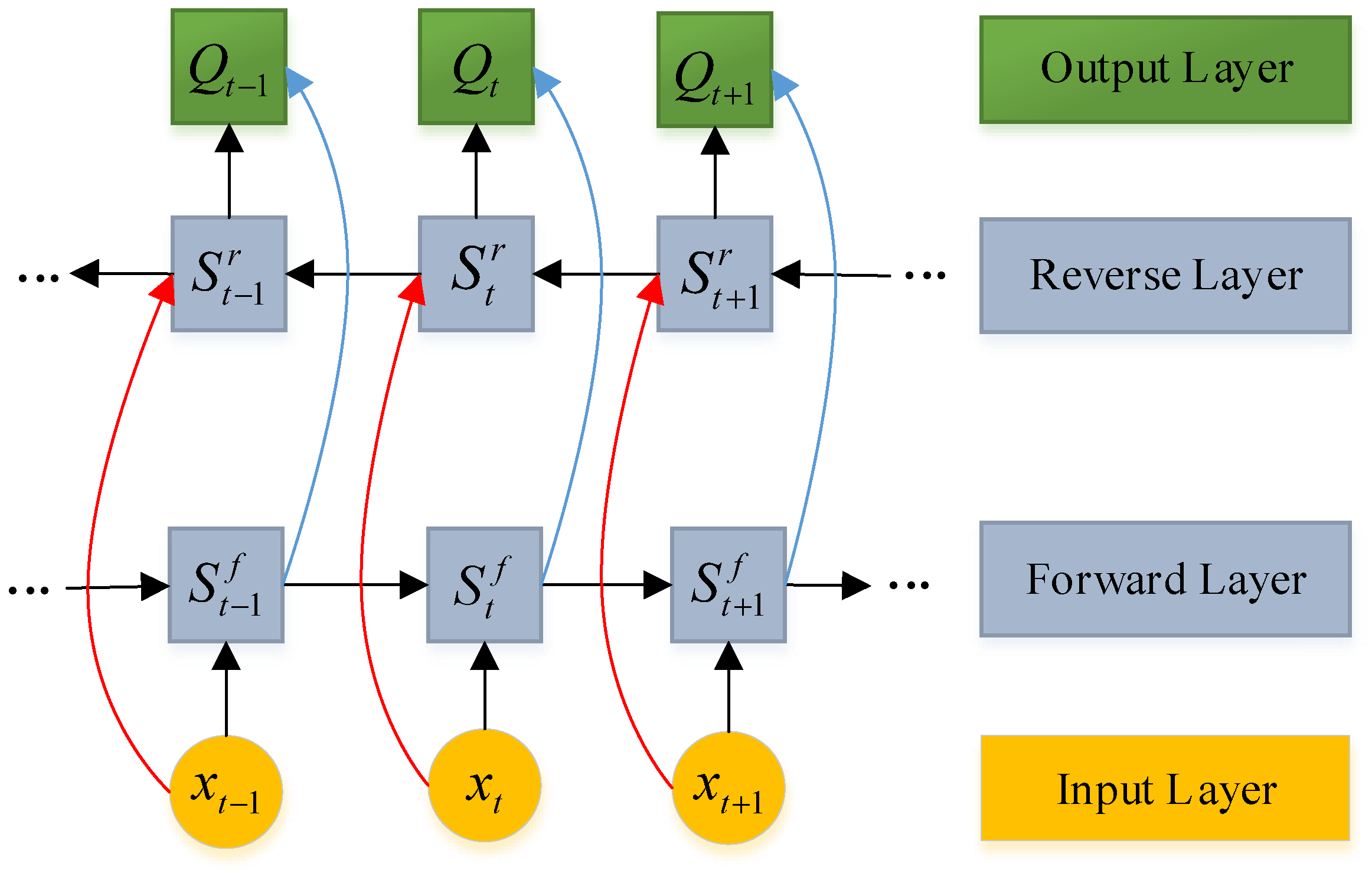
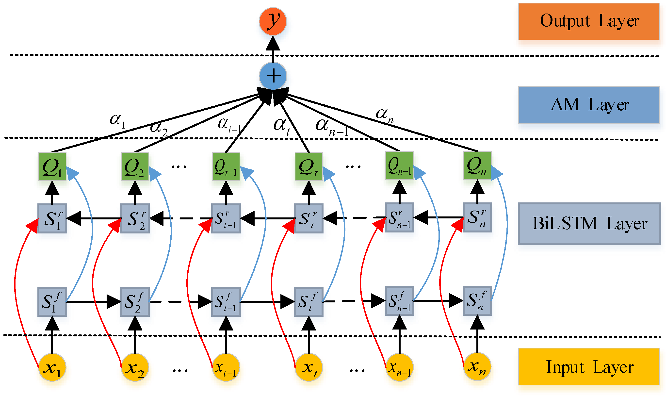
Figure 3 shows the structure of the BiLSTM model. From Figure 3, it can be observed that the BiLSTM model consists of an input layer, forward LSTM, reverse LSTM, and an output layer. The forward LSTM and reverse LSTM can obtain past and future information of the input time-series data, respectively. The output Q t consists of the hidden state s t f of the forward LSTM and the hidden state s t r of the reverse LSTM at time t.
The hidden state s t f of the forward LSTM, the hidden state s t r of the inverse LSTM, and the output layer Q t can be calculated using Equations (6)–(8).
s t f = σ W x s f x t + W s f s f s t 1 f + b s f
s t r = σ W x s f x t + W s r s r s t + 1 r + b s r
Q t = W s f Q s t f + W s r Q s t r + b Q
where σ is the activation function, b is the bias vector, W x s f is the weight matrix of the input layer, W s f s f is the weight matrix of the hidden layer in forward LSTM, and W s r s r is the weight matrix of the hidden layer in reverse LSTM. W s f Q and W s r Q are the weight matrices of the output layer, respectively.

3.3. Attention Mechanism

The attention mechanism (AM) is a resource allocation mechanism that imitates the human brain to process information, ignore irrelevant information, and strengthen required information [39]. The AM assigns a higher degree of attention (weight) to the data points that have a greater impact on photovoltaic power forecasting in the input time series data using probability allocation, and highlights the influence of important data information, thereby improving the accuracy of the forecasting model.
The model structure of the AM is shown in Figure 4, where x t ( t [ 1 ,   n ] ) is the input of BiLSTM, Q t ( t [ 1 ,   n ] ) is the output of the implicit layer obtained for each input after passing through BiLSTM, α t ( t [ 1 ,   n ] ) is the attentional weight (probability allocation value) of the output value of the implicit layer, and y is the output calculated using AM.
where the weight coefficient α t of the AM layer is calculated using Equations (9)–(11).
e t = u tanh ( w Q t + b )
α t = exp ( e t ) i = 1 n exp ( e i )
y = i = 1 t α t Q t
where e t is the value of the attention probability allocation determined by Q t at moment t , u and w are the weight coefficients, and b is the bias coefficient.

3.4. CNN-BiLSTM-AM Model Construction

In this study, the CNN model was used to mine the seasonal characteristics and spatial correlation characteristics between photovoltaic power data and NWP data, and the BiLSTM model was used to mine the temporal correlation of the input data series in order to achieve accurate acquisition of the spatial and temporal distribution characteristics of photovoltaic power data and NWP data, and effectively improve the forecasting accuracy of the BiLSTM model. On this basis, AM is used to assign larger weights to the key elements affecting the forecasting accuracy, which further improves the forecasting accuracy of BiLSTM. The CNN-BiLSTM-AM forecasting model was constructed by combining the advantages of CNN, BiLSTM, and AM to achieve an accurate forecast of day-ahead photovoltaic power. The detailed structure of the CNN-BiLSTM-AM forecasting model is as follows:
(1)
Input layer: The training data were input into the CNN-BiLSTM-AM. The format of the input data is a matrix of N*M, where N is the length of the time-series training data, and M is the data information of each time point in the time-series training data.
(2)
Convolution Layer: The spatial distribution features of the input data were extracted using convolutional operations. The number of convolution kernels is 50, the size of the convolution kernels is 3*3, and the step size is 1.
(3)
Pooling Layer: The input high-dimensional feature data are dimensionally reduced to improve the computational speed and prevent the overfitting of the CNN. In this study, the pooling strategy of max-pooling was used, and the size of the pooling kernel was 2*2 with a step size of 2.
(4)
Fully Connected Layers: A double fully connected layer structure is adopted in this study. The first fully connected layer combines local features in the pooling layer into global features. The second fully connected layer is used as the regression output layer to output a sequence of feature data.
(5)
BiLSTM Layer: mining the temporal correlation of the input data series. Among them, the forward LSTM layer digs the time correlation between the data in a time order. The reverse LSTM layer reversely mines the temporal correlation between the data in the reverse time order. The number of LSTM neurons in the forward and reverse layers is 256.
(6)
Attention Mechanism Layer: adaptively adjust the weight of the calculated value of the BiLSTM model for each input data according to the data order to further improve the forecasting accuracy of the BiLSTM model.
(7)
Output layer: the forecasting results of the CNN-BiLSTM-AM model are output.
The construction process of the CNN-BiLSTM-AM model is illustrated in Figure 5.

4. Gaussian Mixture Model and WT-CNN-BiLSTM-AM-GMM Model Construction

4.1. Gaussian Mixture Model

The Gaussian mixture model (GMM) is a linear combination of a certain number of Gaussian probability density functions to approximate the probability density distribution of the sample set, which has the advantages of high fitting accuracy and fast computation. The probability density functions of GMM are shown in Equations (12)–(14).
P ( x i ) = k = 1 K π k φ ( x i ,   μ k ,   k )
k = 1 K π k = 1
φ x i , μ k , k = 1 2 π D 2 k 1 2 exp 1 2 x i μ k T k 1 x i μ k
In Equations (12)–(14), P ( x i ) is the probability density function of the GMM, x i is the i-th sample in the dataset, π k is the weight of the k-th Gaussian probability density function, μ k and k are the mean and covariance matrix of the k-th Gaussian probability density function, respectively, and D is the dimension of the sample space.
In Equations (12)–(14), there are unknown parameters ( π k , μ k , k ) that need to be solved by sample sets. The common method for solving unknown parameters ( π k , μ k , k ) is the expectation maximization algorithm (EM). The EM algorithm is an iterative algorithm proposed by Dempster et al. [50] in 1977 and is used for the maximum likelihood estimation of parameters of probabilistic models with hidden variables. Each iteration of the EM algorithm consists of two steps: step E is used for expectation and step M is used for maximization. The specific calculation process is as follows.
(1) E-step: calculate the probability that each data x i come from a sub-model k based on the current parameters.
γ i k = π k φ ( x i | μ k , k ) k = 1 K π k φ ( x i | μ k , k ) ,   i = 1 ,   2 ,   ,   N ; k = 1 ,   2 ,   ,   K
In Equation (15), N is the number of samples, and γ i k is the probability that the i-th sample belongs to the k-th Gaussian probability density function.
(2) M-step: calculate the model parameters for a new iteration.
μ k = i = 1 N ( γ i k x i ) i = 1 N ( γ i k ) ,   k = 1 ,   2 ,   ,   K
k = i = 1 N γ i k ( x i μ k ) ( x i μ k ) T i = 1 N γ i k ,   k = 1 ,   2 ,   ,   K
π k = i = 1 N γ i k N ,   k = 1 ,   2 ,   ,   K
(3) The E-step and M-step are repeated until convergence ( θ i + 1 θ i < ε , ε is a small positive real number).

4.2. WT-CNN-BiLSTM-AM-GMM Model Construction

According to the contents of the above sections, a day-ahead photovoltaic power forecasting (PPF) and uncertainty analysis model based on WT-CNN-BiLSTM-AM-GMM was constructed. The realization process of the model is shown in Figure 6. The specific steps are as follows.
(1)
Input the NWP data and the power data of the supervisory control and data acquisition (SCADA) system of wind turbine.
(2)
Normalize all NWP data and photovoltaic power data to [0, 1], and determine the training and testing datasets.
(3)
Divide the normalized training dataset into different datasets according to year, season, and month.
(4)
Perform a wavelet transform on all normalized NWP data and photovoltaic power data.
(5)
The WT-CNN-BiLSTM-AM model is trained and forecasted using various datasets after the wavelet transformation.
(6)
The model forecasting result is reconstructed using a wavelet, and the final forecasting result is obtained.
(7)
The distribution characteristics of the forecasting error are calculated, and the confidence interval of the power forecast is calculated.
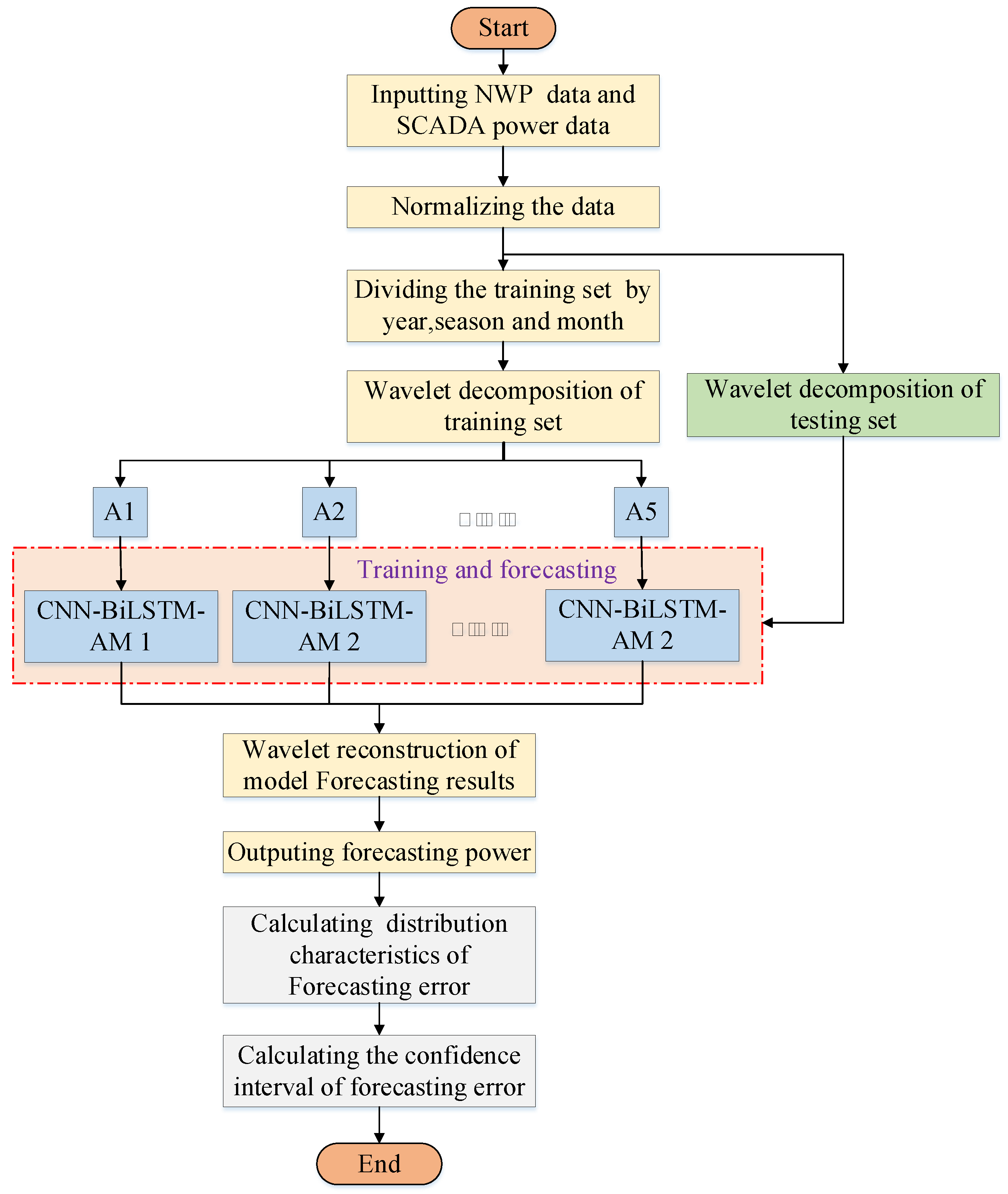
Figure 6. Model construction of WT-CNN-BiLSTM-AM-GMM.
Sustainability 15 06538 g006

5. Case Study

5.1. Data Source

The data used in this study were obtained from a photovoltaic plant in a province in central China with an installed capacity of 2.2 MW, and the time resolution of both NWP data and SCADA data was 10 min. The NWP data include meteorological information, such as wind speed, solar radiation intensity, ambient temperature, and ambient humidity. The SCADA data include the output power data of photovoltaic plant and the temperature data of the solar panel. The data collection time range is the complete year data from 1 January 2015 to 31 December 2015.
During the operation of the photovoltaic power system, its output power is zero when the solar radiation intensity is zero. This part of the data is not helpful for the training and testing of the PPF model and even reduces the forecasting accuracy of the PPF model; therefore, this part of the data needs to be removed. According to the actual operation of the photovoltaic power plant in this study, after removing the data points with zero radiation intensity, the time range of daily valid data was from 7:50 am to 19:50 pm, with a total of 73 data points per day. In addition, after removing the abnormal data caused by factors such as limited power output and photovoltaic power system failure shutdown, the remaining valid dataset has a total of 21,827 data points.

5.2. Training and Testing Dataset

(1)
Testing Dataset
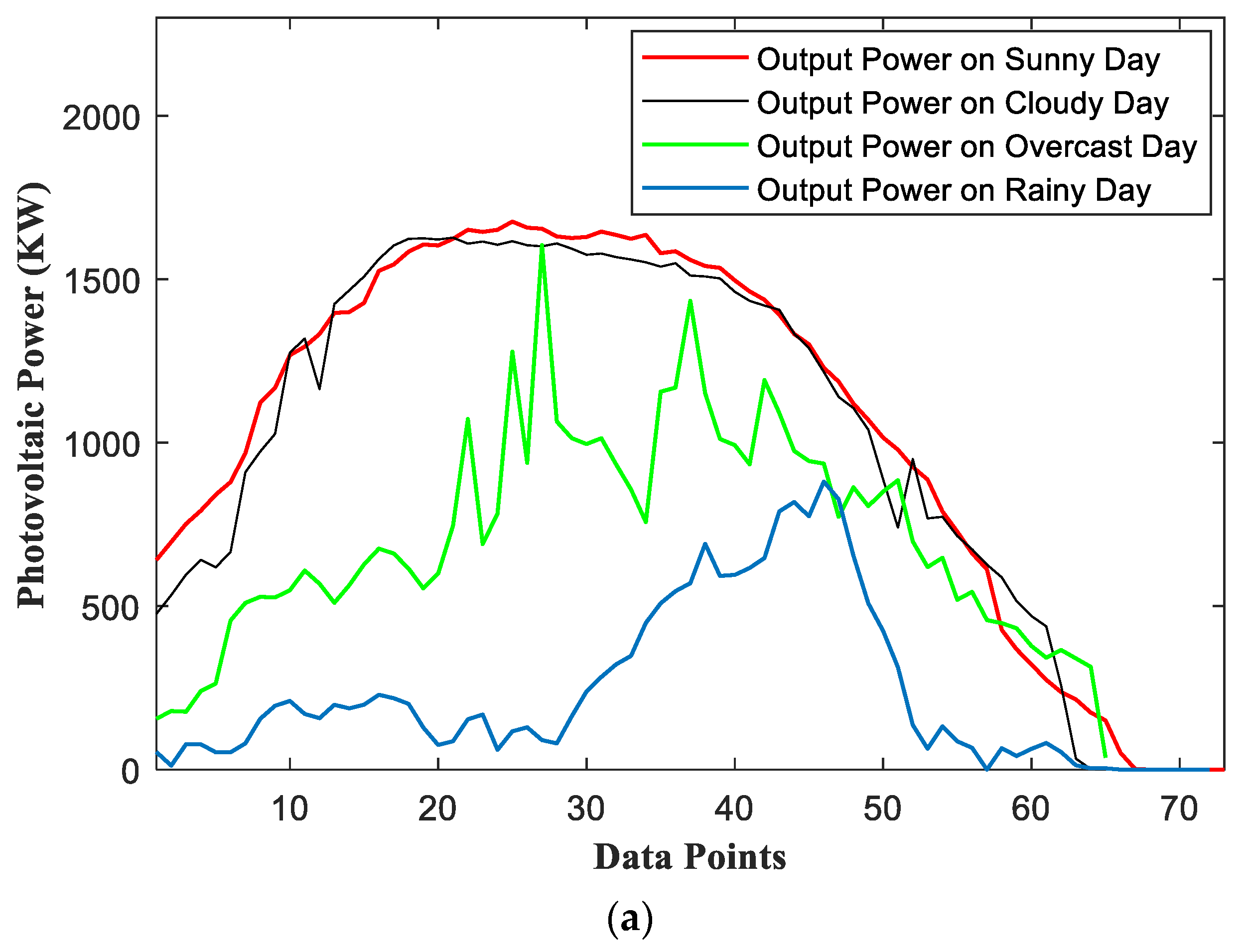
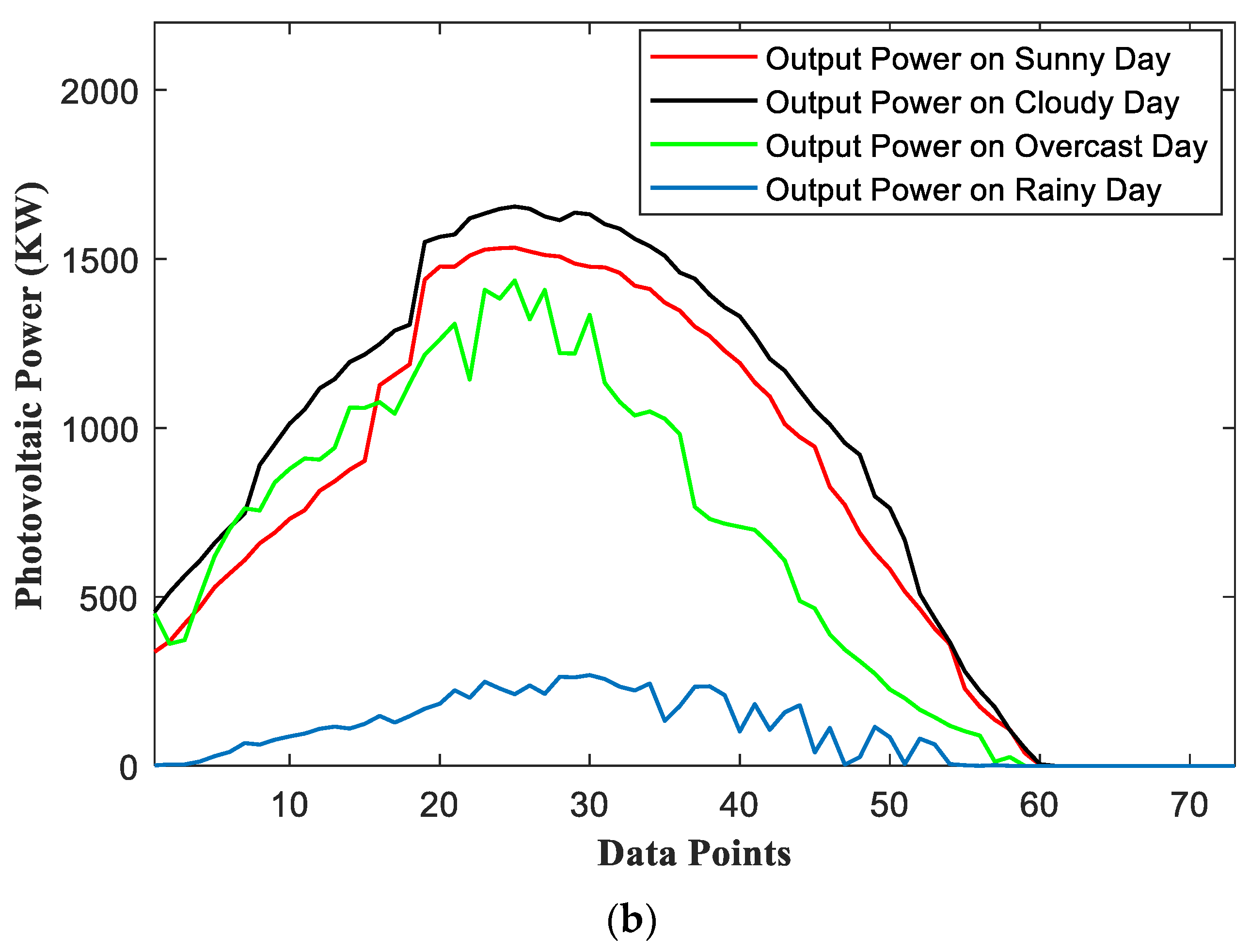
Meteorological conditions are key factors affecting the power output of photovoltaic plants, and different seasons and weather conditions affect the power output of photovoltaic plants. To demonstrate that the WT-CNN-BiLSTM-AM model still has a good forecasting performance under different seasons and weather conditions, this study selected the data under four types of weather conditions (sunny, cloudy, overcast, and rainy days) under different seasons as the testing dataset of the forecasting model. Relevant information for the testing dataset is presented in Table 1 and Figure 7. In Figure 7, the red solid line represents the actual output power of photovoltaic plant under sunny weather, the black solid line represents the actual output power of photovoltaic plant under cloudy weather, the green solid line represents the actual output power of photovoltaic plant under overcast weather, and the blue solid line represents the actual output power of photovoltaic plant under rainy weather.
Table 1. Four weather types and corresponding dates for each season in 2015.
SeasonWeather Type
SunnyCloudyOvercast Rainy
SpringApr. 29thApr. 14thApr. 2ndApr. 19th
SummerAug. 13thAug. 16thAug. 17thAug. 5th
AutumnOct. 12thOct. 9thOct. 3rdOct. 22nd
WinterDec. 17thDec. 15thDec. 8thDec. 21st
Figure 7. Power curves of four weather types in different seasons; (a) Power curves of four weather types in spring; (b) Power curves of the four weather types in autumn.
Sustainability 15 06538 g007aSustainability 15 06538 g007b
Figure 7a shows the actual output power of the photovoltaic plant under four types of weather conditions (sunny, cloudy, overcast, and rainy in spring) and Figure 7b shows the actual output power of photovoltaic plant under four types of weather conditions: sunny, cloudy, overcast, and rainy in autumn. From Figure 7, it can be seen that the output power of photovoltaic power plant in different seasons and under different weather conditions varied greatly. Therefore, the NWP and photovoltaic plant power data under different seasons and weather conditions were selected as the testing dataset to verify the performance of the forecasting model more comprehensively.
(2)
Training Dataset
The remaining data after taking the testing dataset were used as the training dataset, and the training dataset had a total of 20,683 data points. To investigate the effect of the number size of the training dataset on the training effect of the forecasting model, the training dataset was classified according to the following rules.
(a) The remaining data were taken as the training dataset (whole year);
(b) Dividing the remaining data into four training datasets according to seasons;
(c) The remaining data were divided into 12 training datasets according to month.
In the training process, if the testing dataset belongs to a certain month, the training dataset is selected for the corresponding month and season.

5.3. Calculation and Analysis

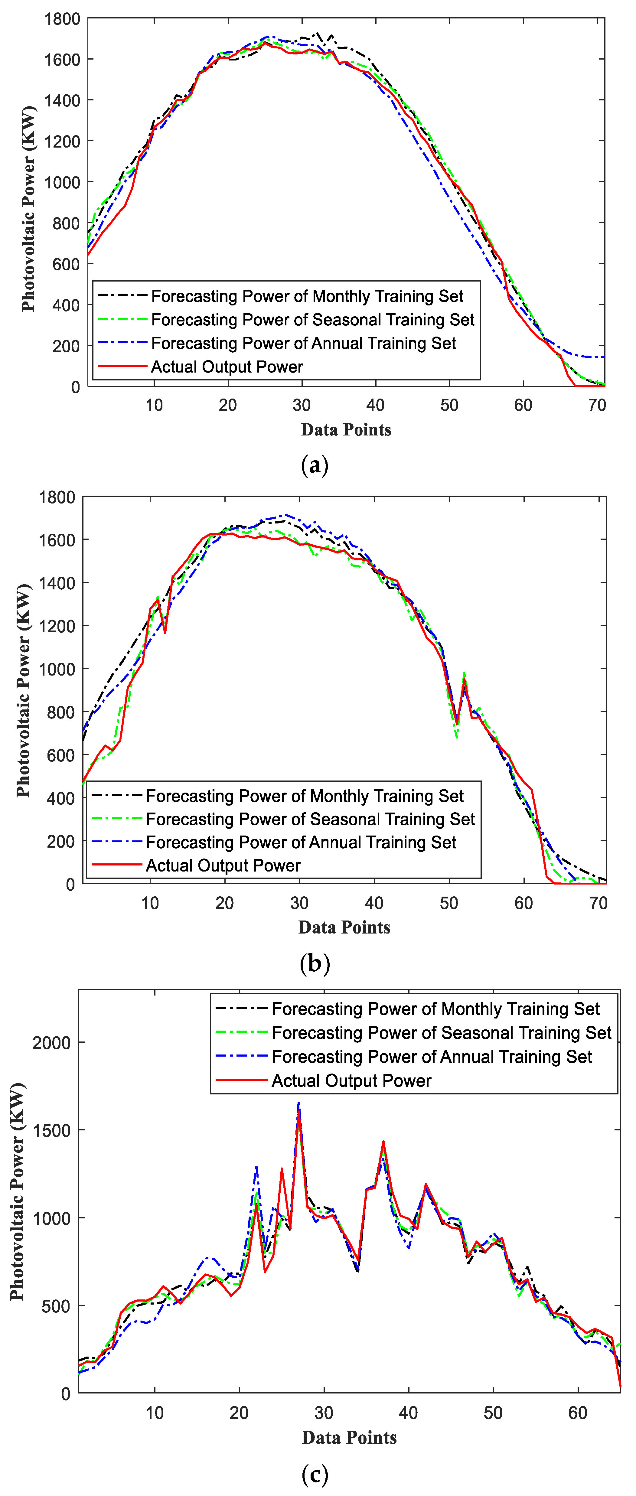
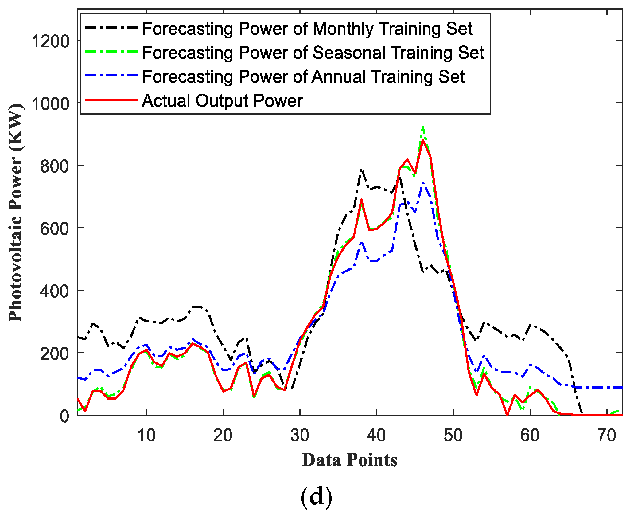
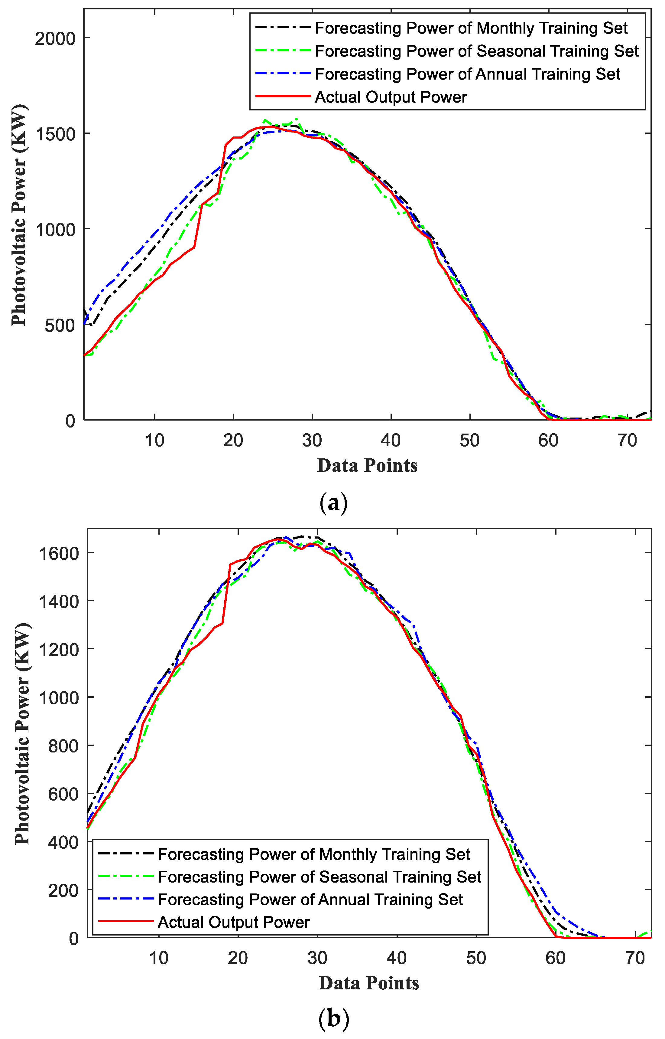
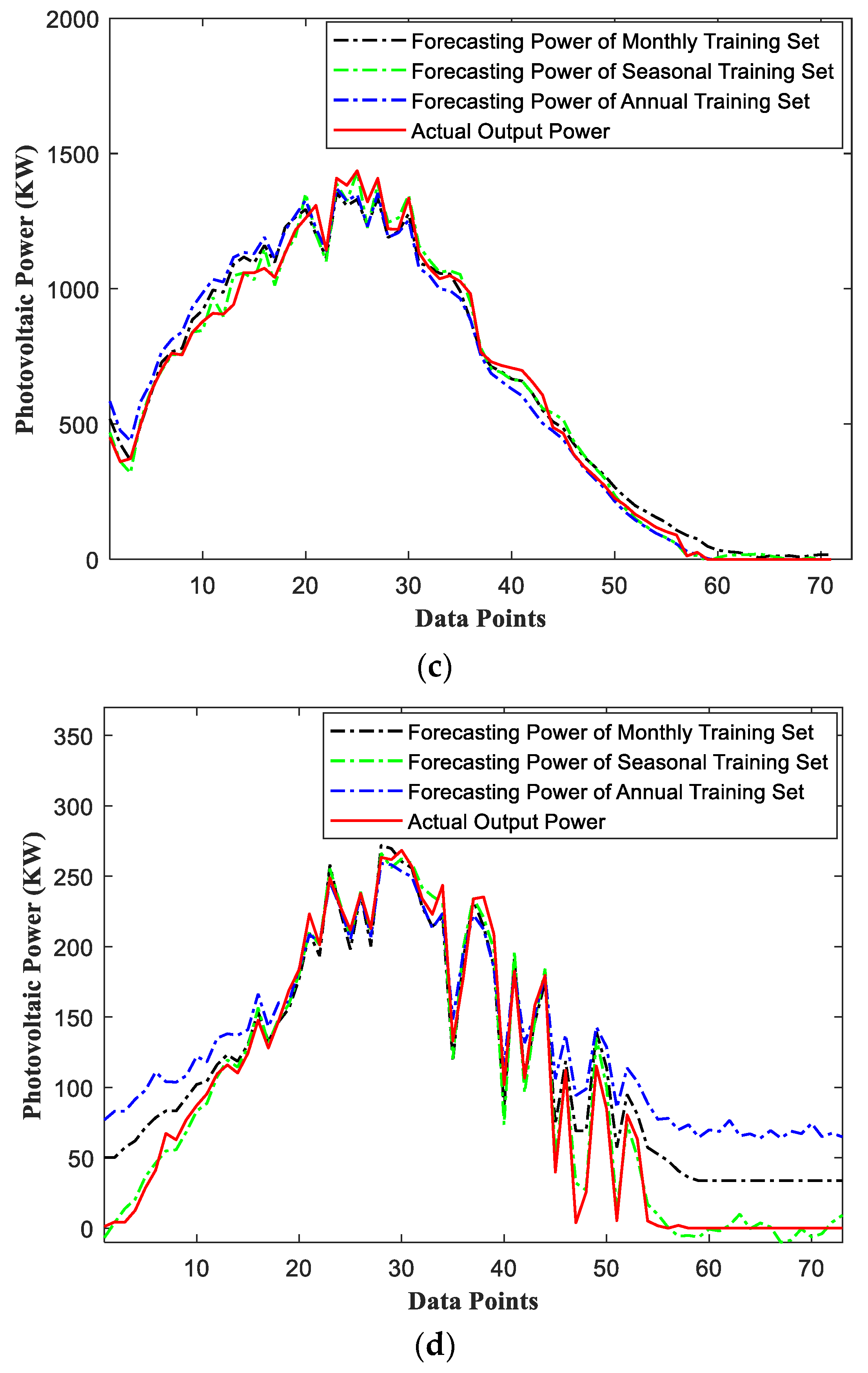
To investigate the effect of training dataset scale size on model forecasting accuracy, this section analyzes the forecasting accuracy of the WT-CNN-BiLSTM-AM model after the training datasets are classified by year, season, and month. Figure 8 and Figure 9 show the forecasting results of the four weather types in spring and autumn under three training datasets: month, season, and year. In Figure 8 and Figure 9, the red solid line is the actual output power of photovoltaic plant, the black dashed line is the forecasting result under the monthly training dataset, the green dashed line is the forecasting result under the seasonal training dataset, and the purple dashed line is the forecasting result for the whole year training dataset.
From Figure 8 and Figure 9, we can see that the WT-CNN-BiLSTM-AM model was trained using the entire year training dataset, seasonal training dataset, and month training dataset, respectively, and the forecasting accuracy of the model under different weather conditions was somewhat different, which indicates that the size of the training dataset affects the forecasting accuracy of the model. However, we also found that the WT-CNN-BiLSTM-AM model can still accurately describe the trend of photovoltaic power under different training dataset scales and weather conditions, which proves that the WT-CNN-BiLSTM-AM model has good forecasting performance.
Table 2 shows the average forecasting error of the trained WT-CNN-BiLSTM-AM model in different seasons under three training dataset scales (the average of the forecasting errors of four weather conditions). From Table 2, it can be seen that the forecasting error value of the WT-CNN-BiLSTM-AM model is the smallest when the training dataset is classified by season, which proves that the training dataset is first classified by season and then the WT-CNN-BiLSTM-AM model is trained to obtain the optimal forecasting accuracy. For this reason, the training dataset classified by season was used in the subsequent training of the WT-CNN-BiLSTM-AM model.

6. Comparison of Different Forecasting Models

From the contents of Section 5, it can be observed that the WT-CNN-BiLSTM-AM model has the highest forecasting accuracy after the training dataset is classified according to season. In future studies, the training dataset will be used after classification according to seasons. To further demonstrate the superiority of the proposed WT-CNN-BiLSTM-AM forecasting model, the forecasting results of CNN-BiLSTM, WT-CNN-BiLSTM, LSTM, gated recurrent unit (GRU), and PSO-BP are compared and analyzed in this section. The training and testing datasets used during the comparative analysis of the forecasting models were consistent with the datasets used in Section 5.
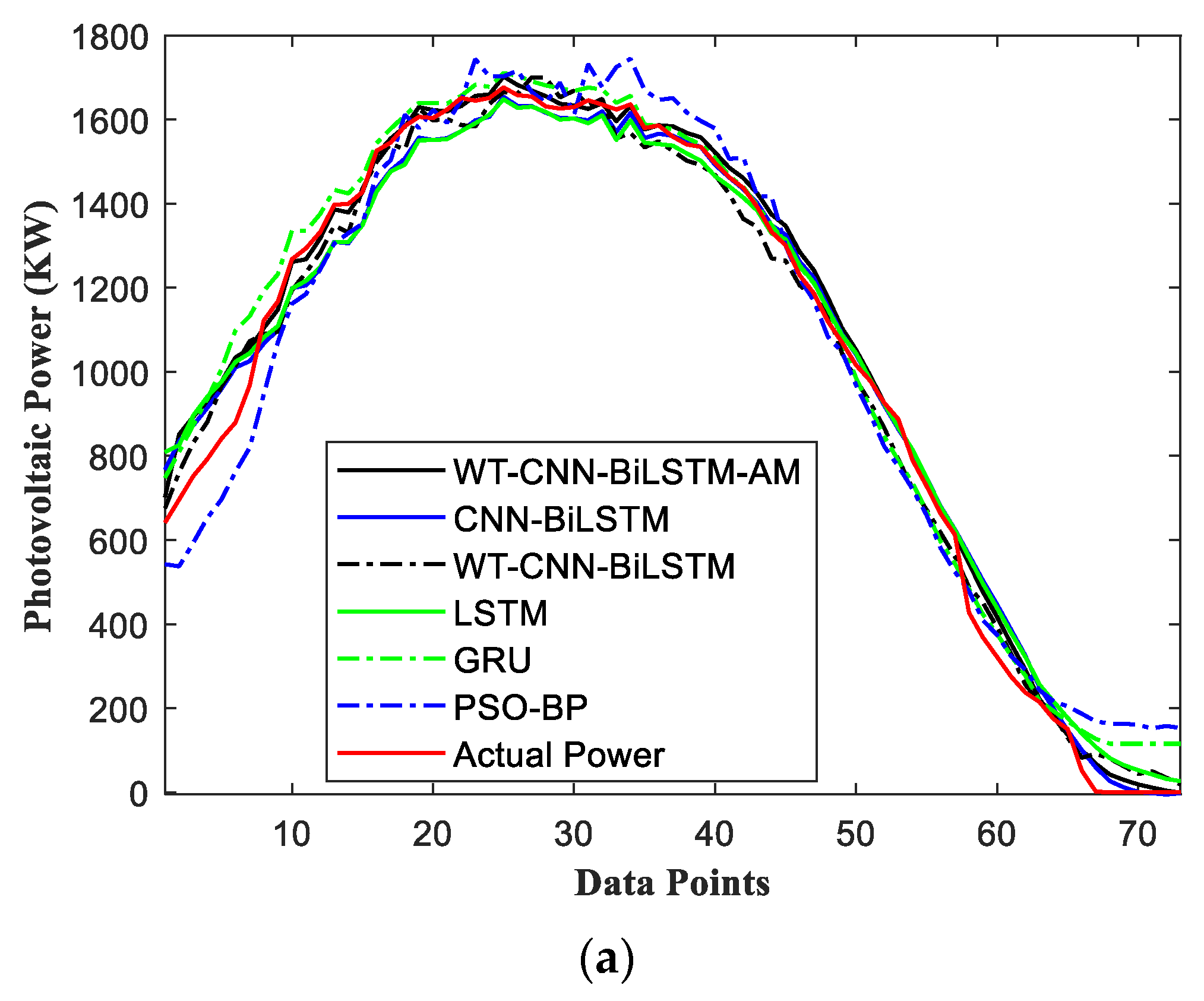
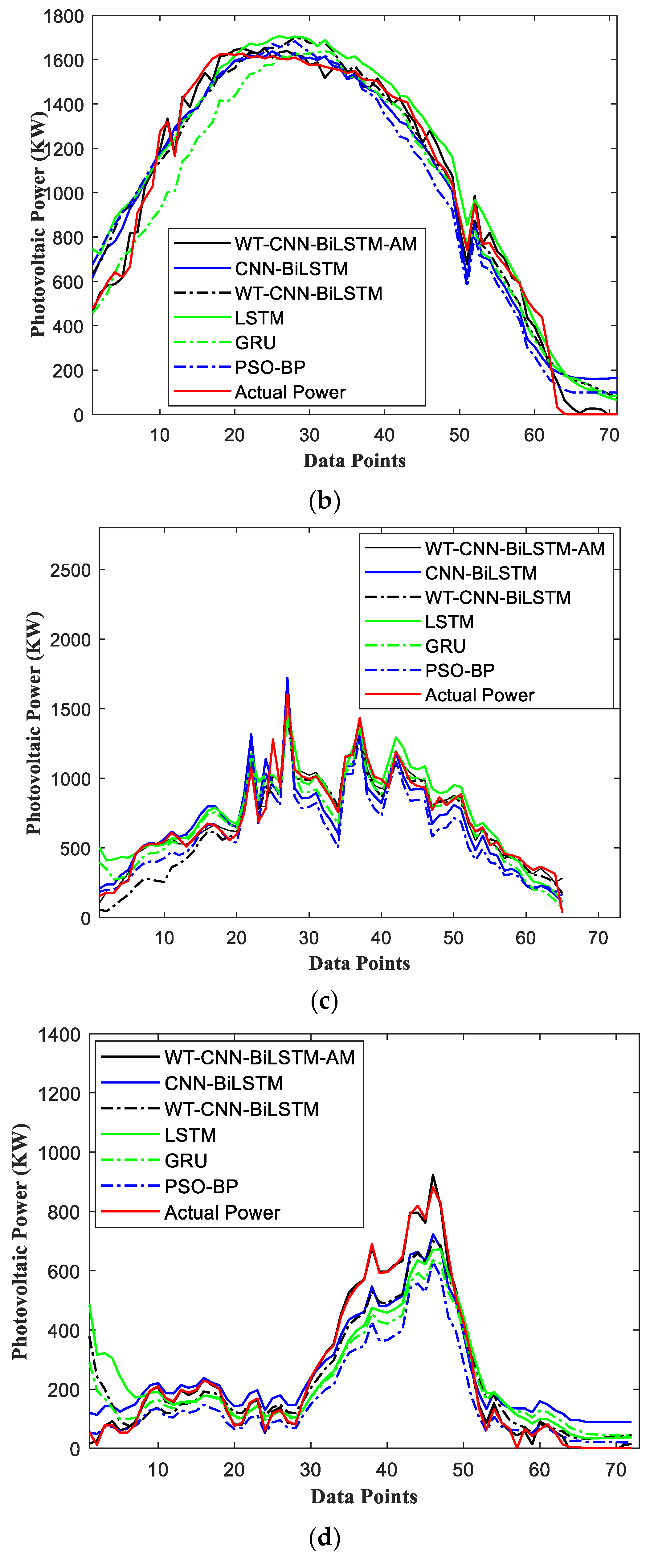
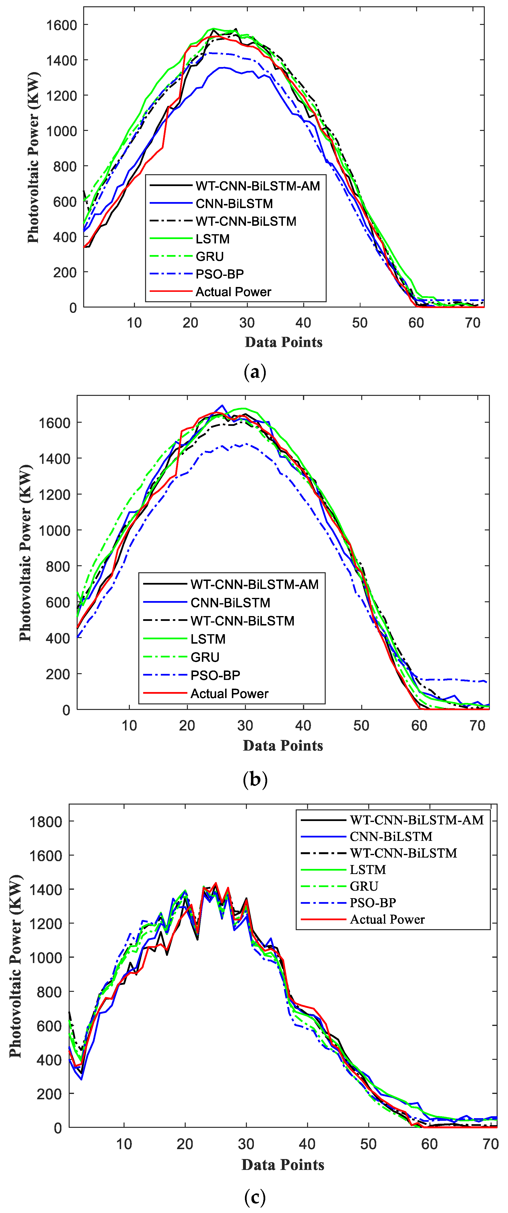
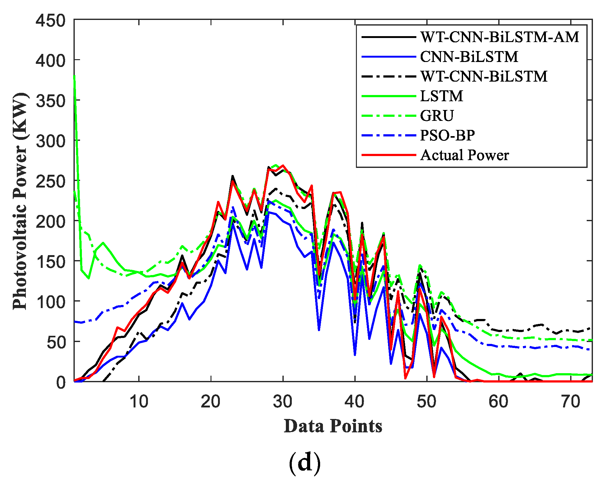
Figure 10 and Figure 11 show the PPF results of various forecasting models for four weather conditions in spring and autumn, where the red solid line is the actual output power of photovoltaic plant, the black solid line represents the forecasting results of the WT-CNN-BiLSTM-AM model, the black dashed line represents the forecasting results of the WT-CNN-BiLSTM model, the blue solid line is the forecasting results of the CNN-BiLSTM model, the blue dashed line is the forecasting results of the PSO-BP model, the green solid line is the forecasting results of the LSTM model, and the green dashed line is the forecasting results of the GRU model.
From Figure 10 and Figure 11, it can be observed that the WT-CNN-BiLSTM-AM, WT-CNN-BiLSTM, CNN-BiLSTM, PSO-BP, LSTM, and GRU can accurately forecast the variation trend of photovoltaic power under different seasons and weather conditions, which proves that the machine learning methods have good forecasting performance for photovoltaic power. We also found that the WT-CNN-BiLSTM-AM model proposed in this paper can describe the trend of photovoltaic power more accurately than those of other forecasting models, which proves that the forecasting performance of the WT-CNN-BiLSTM-AM model is better than that of other models.
Table 3 shows the average values of forecasting errors for each forecasting model under different seasonal conditions (average values of forecasting errors under four weather conditions), where the last row is the average of forecasting errors for all seasons. From Table 3, it can be observed that the WT-CNN-BiLSTM-AM model has the smallest forecasting error value among all forecasting models, which proves that the WT-CNN-BiLSTM-AM model has the highest forecasting accuracy among all forecasting models. The reasonableness and advancement of the WT-CNN-BiLSTM-AM model proposed in this paper was proved.

7. Uncertainty Analysis of PPF

7.1. Probability Density Estimation of PPF Error

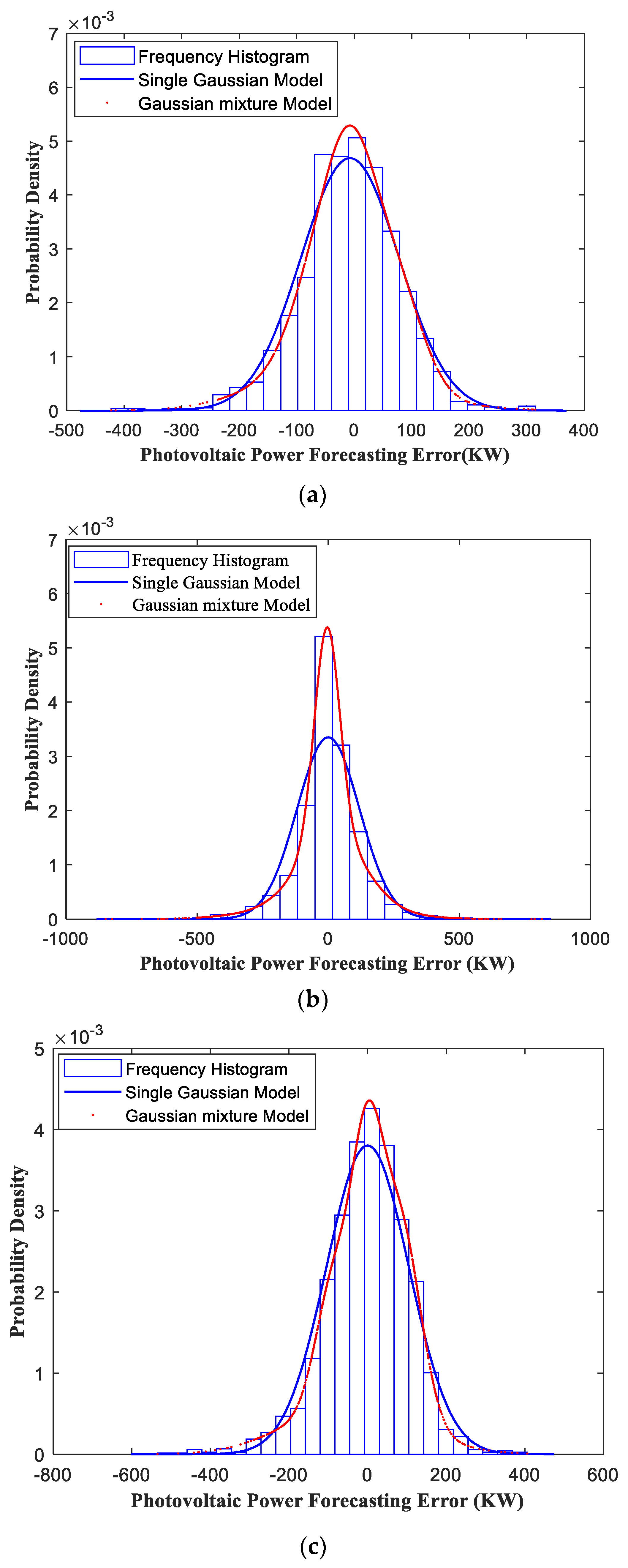
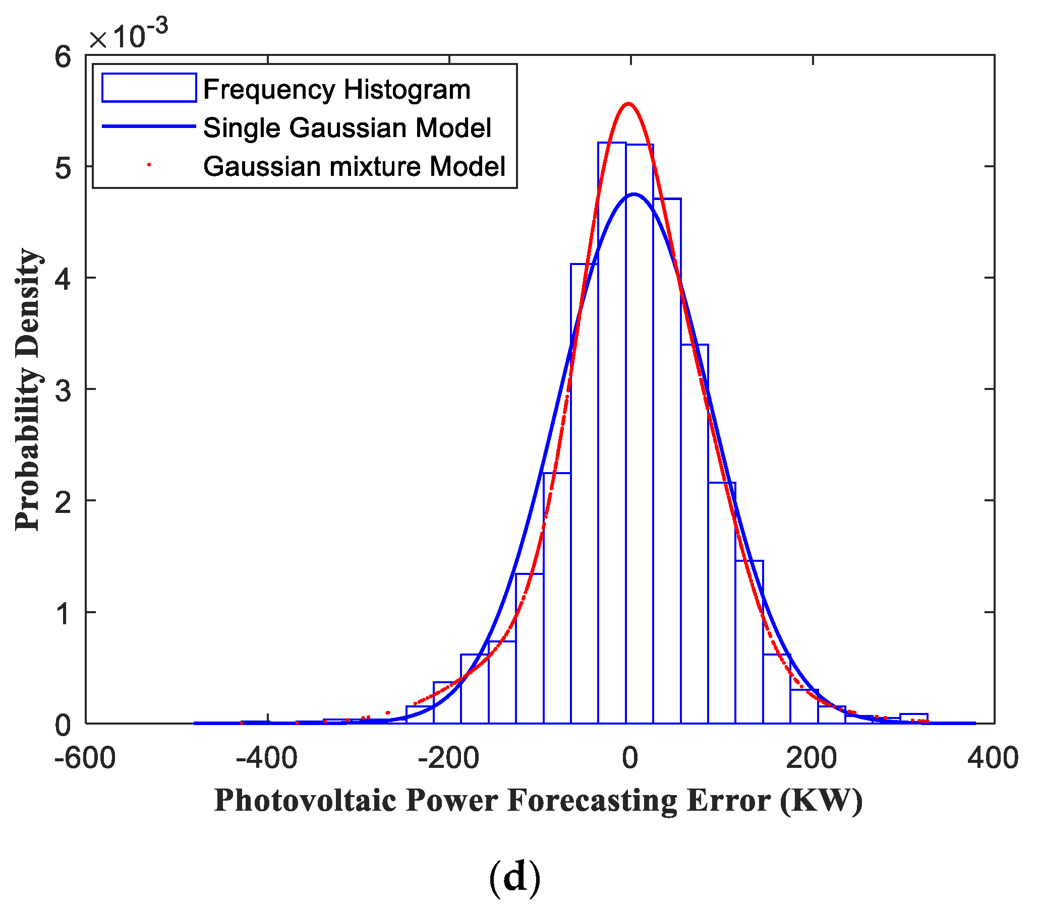
When using the confidence interval to describe the distribution range of the PPF, it is first necessary to determine the probability density distribution characteristics of the PPF errors. This study uses the Gaussian mixture model (GMM) in Section 4.1 to calculate the probability density distribution of PPF errors.
Figure 12 shows the probability density distribution of the PPF errors in the spring. In Figure 12, the histogram indicates the distribution characteristics of PPF errors: the blue curve is the probability density distribution of PPF errors obtained from a single Gaussian model; and the red curve is the probability density distribution of PPF errors obtained from GMM. From Figure 12, it can be seen that the probability density curve of PPF errors obtained from the GMM can more accurately describe the distribution characteristics of PPF errors.

7.2. Confidence Intervals of PPF

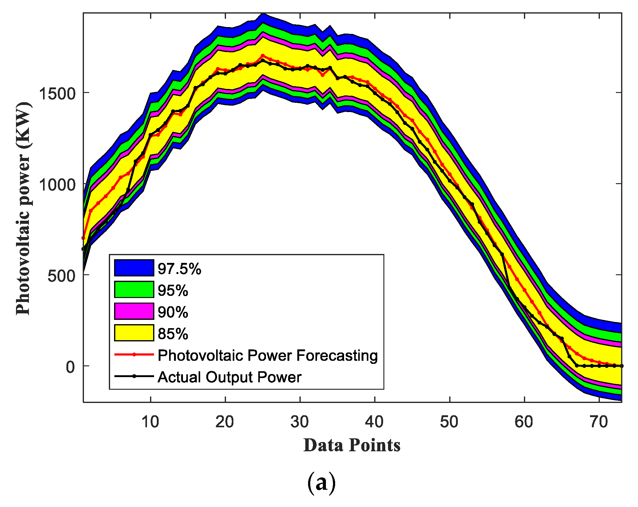
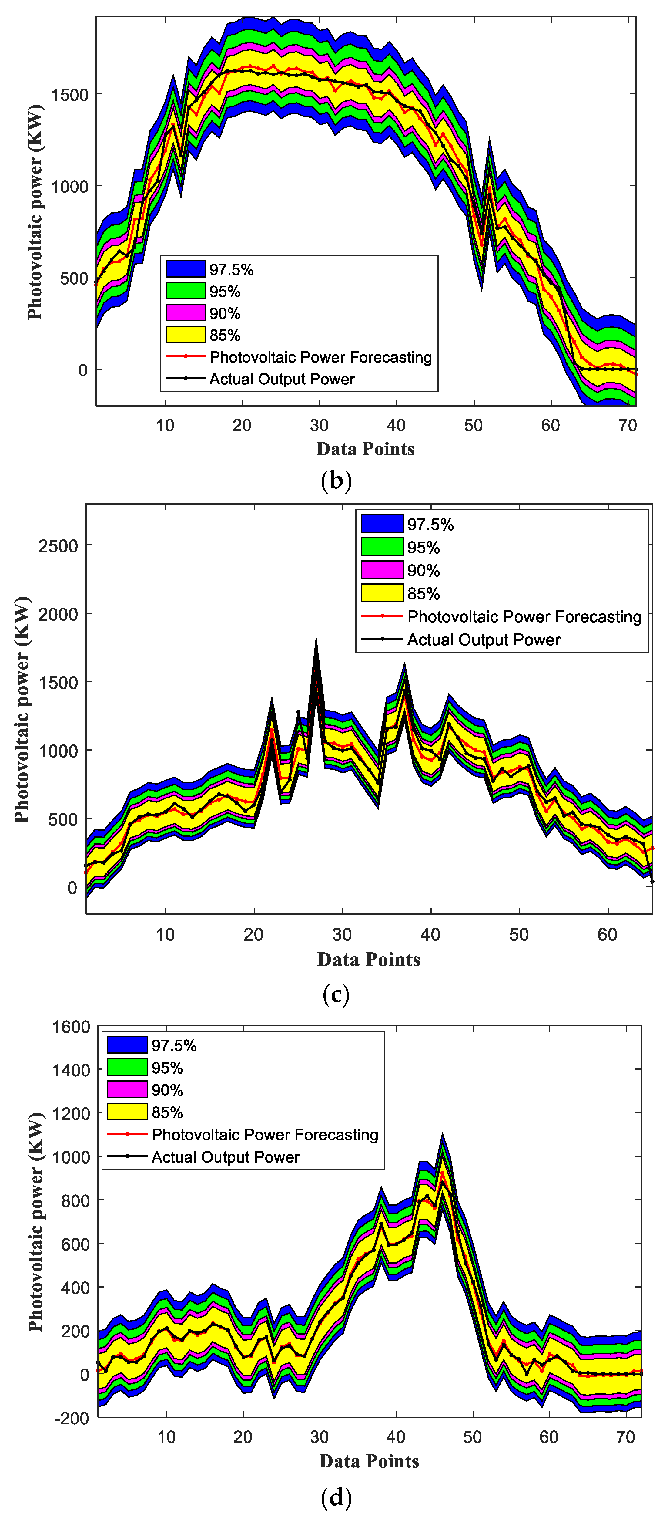
After obtaining the probability density distribution of PPF errors using GMM, the confidence interval can be used to calculate the uncertainty distribution range of the PPF. The confidence interval distributions of the proposed WT-CNN-BiLSTM-AM model in spring at the 97.5%, 95%, 90%, and 85% confidence levels are shown in Figure 13. In Figure 13, the red solid line represents the forecasting power of the WT-CNN-BiLSTM-AM model, and the black solid line represents the actual output power of the photovoltaic plant. From Figure 13, it can be seen that under different weather types, although a very small portion of the actual photovoltaic power values do not fall within the confidence interval (owing to factors such as NWP errors and sudden changes in weather, the actual output power is quite different from the forecasting power), the overall real photovoltaic power values still fall within the confidence interval with a probability greater than the confidence level, proving that the GMM can accurately calculate the probability density distribution characteristics of PPF errors.
Table 4 shows the coverage of PPF confidence intervals of WT-CNN-BiLSTM-AM model. It can be seen from Table 4 that, except the coverage of PPF confidence interval on October 12 in autumn, which is slightly lower than the confidence level (blue font in Table 4), the coverage of PPF confidence interval is higher than the confidence level in other times. It is verified that the GMM can accurately calculate the distribution characteristics of PPF errors under different seasons and weather conditions.

8. Conclusions

In this study, a day-ahead photovoltaic power forecasting model based on the WT-CNN-BiLSTM-AM-GMM method is proposed. First, the NWP data and photovoltaic power data are decomposed into frequency data with time information using WT to eliminate the impact of randomness and volatility in data information on forecasting accuracy. Second, the WT-CNN-BiLSTM-AM model was constructed by integrating the advantages of the CNN, BiLSTM, and AM models. To accurately calculate the probability density distribution characteristics of forecasting errors, the GMM method was used to calculate the probability density distribution of forecasting errors, and the confidence interval of the day-ahead photovoltaic power forecasting was calculated. The calculation results are as follows.
(1)
WT is used to decompose NWP data and photovoltaic power data into frequency data with time information, which can effectively eliminate the impact of randomness and volatility in data information on forecasting accuracy and improve the accuracy of the forecasting model.
(2)
The WT-CNN-BiLSTM-AM model can effectively mine the spatial and temporal correlation characteristics of the training dataset and improve the forecasting accuracy of the model.
(3)
The forecasting accuracies of WT-CNN-BiLSTM-AM, CNN-BiLSTM, WT-CNN-BiLSTM, LSTM, GRU, and PSO-BP were compared and analyzed, and it was found that under different seasons and weather conditions, the forecasting accuracy of the WT-CNN-BiLSTM-AM model was higher than that of the other models.
(4)
The GMM was used to calculate the probability density distribution characteristics of photovoltaic power forecasting errors, and the confidence interval and the coverage of the confidence interval of photovoltaic power forecasting were calculated accordingly. The calculations show that the GMM can accurately describe the probability density distribution characteristics of photovoltaic power forecasting errors compared to the single Gaussian model.

Author Contributions

Conceptualization, B.G.; methodology, B.G.; software, X.L.; validation, X.L.; formal analysis, X.L.; investigation, F.X., X.Y., F.W. and P.W.; resources, F.X., X.Y. and F.W.; data curation, F.X., X.Y. and F.W.; writing—original draft preparation, B.G.; writing—review and editing, B.G.; visualization, X.Y. and P.W.; supervision, B.G.; project administration, B.G.; funding acquisition, B.G. All authors have read and agreed to the published version of the manuscript.

Funding

This work was supported by the National Key Research and Development Program of China [grant number 2019YFE0104800].

Institutional Review Board Statement

Not applicable.

Informed Consent Statement

Not applicable.

Data Availability Statement

Not applicable.

Acknowledgments

The authors thank the editors and reviewers for their helpful comments regarding the manuscript and other individuals who contributed but are not listed as authors of this study.

Conflicts of Interest

The authors declare no conflict of interest.

References

  1. IRENA. Renewable Energy Statistics. 2021. Available online: https://www.irena.org/publications/2021/March/RenewableCapacityStatistics2021 (accessed on 31 March 2021).
  2. Ahmed, R.; Sreeram, V.; Mishra, Y.; Arif, M. A review and evaluation of the state-of-the-art in PV solar power forecasting: Techniques and optimization. Renew. Sustain. Energy Rev. 2020, 124, 109792. [Google Scholar] [CrossRef]
  3. Antonanzas, J.; Osorio, N.; Escobar, R.; Urraca, R.; Martinez-De-Pison, F.J.; Antonanzas-Torres, F. Review of photovoltaic power forecasting. Sol. Energy 2016, 136, 78–111. [Google Scholar] [CrossRef]
  4. Yang, D.; Kleissl, J.; Gueymard, C.A.; Pedro, H.T.; Coimbra, C.F. History and trends in solar irradiance and PV power forecasting: A preliminary assessment and review using text mining. Sol. Energy 2018, 168, 60–101. [Google Scholar] [CrossRef]
  5. Han, S.; Qiao, Y.-H.; Yan, J.; Liu, Y.-Q.; Li, L.; Wang, Z. Mid-to-long term wind and photovoltaic power generation prediction based on copula function and long short term memory network. Appl. Energy 2019, 239, 181–191. [Google Scholar] [CrossRef]
  6. Ding, S.; Li, R.; Tao, Z. A novel adaptive discrete grey model with time-varying parameters for long-term photovoltaic power generation forecasting. Energy Convers. Manag. 2020, 227, 113644. [Google Scholar] [CrossRef]
  7. Hassan, M.A.; Bailek, N.; Bouchouicha, K.; Nwokolo, S.C. Ultra-short-term exogenous forecasting of photovoltaic power production using genetically optimized non-linear auto-regressive recurrent neural networks. Renew. Energy 2021, 171, 191–209. [Google Scholar] [CrossRef]
  8. Sobrina, S.; Sam, K.K.; Nasrudin, A.R. Solar Photovoltaic Generation Forecasting Methods: A Review. Energy Convers. Manag. 2018, 156, 459–497. [Google Scholar] [CrossRef]
  9. Das, U.K.; Tey, K.S.; Seyedmahmoudian, M.; Mekhilef, S.; Idris, M.Y.I.; Van Deventer, W.; Horan, B.; Stojcevski, A. Forecasting of photovoltaic power generation and model optimization: A review. Renew. Sustain. Energy Rev. 2018, 81, 912–928. [Google Scholar] [CrossRef]
  10. Ramirez-Vergara, J.; Bosman, L.B.; Wollega, E.; Leon-Salas, W.D. Review of Forecasting Methods to Support Photovoltaic Predictive Maintenance. Clean. Eng. Technol. 2022, 8, 100460. [Google Scholar] [CrossRef]
  11. Mayer, M.J. Influence of design data availability on the accuracy of physical photovoltaic power forecasts. Sol. Energy 2021, 227, 532–540. [Google Scholar] [CrossRef]
  12. Mayer, M.J.; Gróf, G. Extensive comparison of physical models for photovoltaic power forecasting. Appl. Energy 2021, 283, 116239. [Google Scholar] [CrossRef]
  13. Ramadhan, R.A.; Heatubun, Y.R.; Tan, S.F.; Lee, H.-J. Comparison of physical and machine learning models for estimating solar irradiance and photovoltaic power. Renew. Energy 2021, 178, 1006–1019. [Google Scholar] [CrossRef]
  14. van der Meer, D.; Widén, J.; Munkhammar, J. Review on probabilistic forecasting of photovoltaic power production and electricity consumption. Renew. Sustain. Energy Rev. 2018, 81, 1484–1512. [Google Scholar] [CrossRef]
  15. Dubey, A.K.; Kumar, A.; García-Díaz, V.; Sharma, A.K.; Kanhaiya, K. Study and analysis of SARIMA and LSTM in forecasting time series data. Sustain. Energy Technol. Assess. 2021, 47, 101474. [Google Scholar] [CrossRef]
  16. Belmahdi, B.; Louzazni, M.; El Bouardi, A. One month-ahead forecasting of mean daily global solar radiation using time series models. Optik 2020, 219, 165207. [Google Scholar] [CrossRef]
  17. AlShafeey, M.; Csáki, C. Evaluating neural network and linear regression photovoltaic power forecasting models based on different input methods. Energy Rep. 2021, 7, 7601–7614. [Google Scholar] [CrossRef]
  18. David, M.; Martin, J.M. Comparison of Machine Learning Methods for Photovoltaic Power Forecasting Based on Numerical Weather Prediction. Renew. Sustain. Energy Rev. 2022, 161, 112364. [Google Scholar]
  19. Akhter, M.N.; Mekhilef, S.; Mokhlis, H.; Shah, N.M. Review on forecasting of photovoltaic power generation based on machine learning and metaheuristic techniques. IET Renew. Power Gener. 2019, 13, 1009–1023. [Google Scholar] [CrossRef] [Green Version]
  20. Gu, B.; Shen, H.; Lei, X.; Hu, H.; Liu, X. Forecasting and uncertainty analysis of day-ahead photovoltaic power using a novel forecasting method. Appl. Energy 2021, 299, 117291. [Google Scholar] [CrossRef]
  21. Wang, X.; Sun, Y.; Luo, D.; Peng, J. Comparative study of machine learning approaches for predicting short-term photovoltaic power output based on weather type classification. Energy 2021, 240, 122733. [Google Scholar] [CrossRef]
  22. Wang, J.; Zhou, Y.; Li, Z. Hour-ahead photovoltaic generation forecasting method based on machine learning and multi objective optimization algorithm. Appl. Energy 2022, 312, 118725. [Google Scholar] [CrossRef]
  23. Rodríguez, F.; Martín, F.; Fontán, L.; Galarza, A. Ensemble of machine learning and spatiotemporal parameters to forecast very short-term solar irradiation to compute photovoltaic generators’ output power. Energy 2021, 229, 120647. [Google Scholar] [CrossRef]
  24. Li, B.; Delpha, C.; Diallo, D.; Migan-Dubois, A. Application of Artificial Neural Networks to photovoltaic fault detection and diagnosis: A review. Renew. Sustain. Energy Rev. 2021, 138, 110512. [Google Scholar] [CrossRef]
  25. Pazikadin, A.R.; Rifai, D.; Ali, K.; Malik, M.Z.; Abdalla, A.N.; Faraj, M.A. Solar irradiance measurement instrumentation and power solar generation forecasting based on Artificial Neural Networks (ANN): A review of five years research trend. Sci. Total Environ. 2020, 715, 136848. [Google Scholar] [CrossRef] [PubMed]
  26. Natarajan, Y.; Kannan, S.; Selvaraj, C.; Mohanty, S.N. Forecasting energy generation in large photovoltaic plants using radial belief neural network. Sustain. Comput. Inform. Syst. 2021, 31, 100578. [Google Scholar] [CrossRef]
  27. Moreira, M.; Balestrassi, P.; Paiva, A.; Ribeiro, P.; Bonatto, B. Design of experiments using artificial neural network ensemble for photovoltaic generation forecasting. Renew. Sustain. Energy Rev. 2020, 135, 110450. [Google Scholar] [CrossRef]
  28. Ma, X.; Zhang, X. A short-term prediction model to forecast power of photovoltaic based on MFA-Elman. Energy Rep. 2022, 8, 495–507. [Google Scholar] [CrossRef]
  29. Kumari, P.; Toshniwal, D. Deep learning models for solar irradiance forecasting: A comprehensive review. J. Clean. Prod. 2021, 318, 128566. [Google Scholar] [CrossRef]
  30. Aslam, S.; Herodotou, H.; Mohsin, S.M.; Javaid, N.; Ashraf, N.; Aslam, S. A survey on deep learning methods for power load and renewable energy forecasting in smart microgrids. Renew. Sustain. Energy Rev. 2021, 144, 110992. [Google Scholar] [CrossRef]
  31. Wang, H.; Lei, Z.; Zhang, X.; Zhou, B.; Peng, J. A review of deep learning for renewable energy forecasting. Energy Convers. Manag. 2019, 198, 111799. [Google Scholar] [CrossRef]
  32. Etxegarai, G.; López, A.; Aginako, N.; Rodríguez, F. An Analysis of Different Deep Learning Neural Networks for Intra-hour Solar Irradiation Forecasting to Compute Solar Photovoltaic Generators’ Energy Production. Energy Sustain. Dev. 2022, 68, 1–17. [Google Scholar] [CrossRef]
  33. Mellit, A.; Pavan, A.M.; Lughi, V. Deep learning neural networks for short-term photovoltaic power forecasting. Renew. Energy 2021, 172, 276–288. [Google Scholar] [CrossRef]
  34. Zang, H.; Cheng, L.; Ding, T.; Cheung, K.W.; Wei, Z.; Sun, G. Day-ahead photovoltaic power forecasting approach based on deep convolutional neural networks and meta learning. Int. J. Electr. Power Energy Syst. 2020, 118, 105790. [Google Scholar] [CrossRef]
  35. Huang, X.; Li, Q.; Tai, Y.; Chen, Z.; Zhang, J.; Shi, J.; Gao, B.; Liu, W. Hybrid deep neural model for hourly solar irradiance forecasting. Renew. Energy 2021, 171, 1041–1060. [Google Scholar] [CrossRef]
  36. Lai, C.S.; Zhong, C.; Pan, K.; Ng, W.W.; Lai, L.L. A deep learning based hybrid method for hourly solar radiation forecasting. Expert Syst. Appl. 2021, 177, 114941. [Google Scholar] [CrossRef]
  37. Tang, Y.; Yang, K.; Zhang, S.; Zhang, Z. Photovoltaic power forecasting: A hybrid deep learning model incorporating transfer learning strategy. Renew. Sustain. Energy Rev. 2022, 162, 112473. [Google Scholar] [CrossRef]
  38. Qu, J.; Qian, Z.; Pei, Y. Day-ahead hourly photovoltaic power forecasting using attention-based CNN-LSTM neural network embedded with multiple relevant and target variables prediction pattern. Energy 2021, 232, 120996. [Google Scholar] [CrossRef]
  39. Khan, W.; Walker, S.; Zeiler, W. Improved solar photovoltaic energy generation forecast using deep learning-based ensemble stacking approach. Energy 2022, 240, 122812. [Google Scholar] [CrossRef]
  40. Akhter, M.N.; Mekhilef, S.; Mokhlis, H.; Ali, R.; Usama, M.; Muhammad, M.A.; Khairuddin, A.S.M. A hybrid deep learning method for an hour ahead power output forecasting of three different photovoltaic systems. Appl. Energy 2021, 307, 118185. [Google Scholar] [CrossRef]
  41. Akhter, M.N.; Mekhilef, S.; Mokhlis, H.; Almohaimeed, Z.M.; Muhammad, M.A.; Khairuddin, A.S.M.; Akram, R.; Hussain, M.M. An Hour-Ahead PV Power Forecasting Method Based on an RNN-LSTM Model for Three Different PV Plants. Energies 2022, 15, 2243. [Google Scholar] [CrossRef]
  42. Wen, X.; Abbes, D.; Francois, B. Modeling of photovoltaic power uncertainties for impact analysis on generation scheduling and cost of an urban micro grid. Math. Comput. Simul. 2020, 183, 116–128. [Google Scholar] [CrossRef]
  43. Liu, L.; Zhao, Y.; Chang, D.; Xie, J.; Ma, Z.; Sun, Q.; Yin, H.; Wennersten, R. Prediction of short-term PV power output and uncertainty analysis. Appl. Energy 2018, 228, 700–711. [Google Scholar] [CrossRef]
  44. von Loeper, F.; Schaumann, P.; de Langlard, M.; Hess, R.; Bäsmann, R.; Schmidt, V. Probabilistic prediction of solar power supply to distribution networks, using forecasts of global horizontal irradiation. Sol. Energy 2020, 203, 145–156. [Google Scholar] [CrossRef]
  45. Bozorg, M.; Bracale, A.; Carpita, M.; De Falco, P.; Mottola, F.; Proto, D. Bayesian bootstrapping in real-time probabilistic photovoltaic power forecasting. Sol. Energy 2021, 225, 577–590. [Google Scholar] [CrossRef]
  46. Schinke-Nendza, A.; von Loeper, F.; Osinski, P.; Schaumann, P.; Schmidt, V.; Weber, C. Probabilistic forecasting of photovoltaic power supply—A hybrid approach using D-vine copulas to model spatial dependencies. Appl. Energy 2021, 304, 117599. [Google Scholar] [CrossRef]
  47. Yang, M.; Zhu, L. Short-term Prediction Error Analysis of Photovoltaic Power Based on Non-Parametric Estimation. Power Grids Clean Energy 2020, 36, 107–114. [Google Scholar]
  48. Koenker, R.; Bassett, G. Regression Quantiles. Econometrica 1978, 46, 33–50. [Google Scholar] [CrossRef]
  49. Sugiyama, S. Forecast Uncertainty and Monte Carlo Simulation. Foresight Int. J. Appl. Forecast. 2007, 29–37. Available online: https://econpapers.repec.org/article/forijafaa/ (accessed on 31 March 2021).
  50. Watanabe, T.; Nohara, D. Prediction of time series for several hours of surface solar irradiance using one-granule cloud property data from satellite observations. Sol. Energy 2019, 186, 113–125. [Google Scholar] [CrossRef]
  51. Savkin, A.V.; Petersen, I.R. Robust filtering with missing data and a deterministic description of noise and uncertainty. Int. J. Syst. Sci. 1997, 28, 373–378. [Google Scholar] [CrossRef]
  52. Natapol, K.; Thananchai, L. Uncertainty via Statistical Interpretation of Multiple Forecasting Models. Energy 2019, 180, 387–397. [Google Scholar]
  53. Peng, C.; Zou, J.; Zhang, Z.; Han, L.; Liu, M. An Ultra-Short-Term Pre-Plan Power Curve based Smoothing Control Approach for Grid-connected Wind-Solar-Battery Hybrid Power System. IFAC-PapersOnLine 2017, 50, 7711–7716. [Google Scholar] [CrossRef]
  54. Yu, C.; Li, Y.; Zhang, M. An improved Wavelet Transform using Singular Spectrum Analysis for wind speed forecasting based on Elman Neural Network. Energy Convers. Manag. 2017, 148, 895–904. [Google Scholar] [CrossRef]
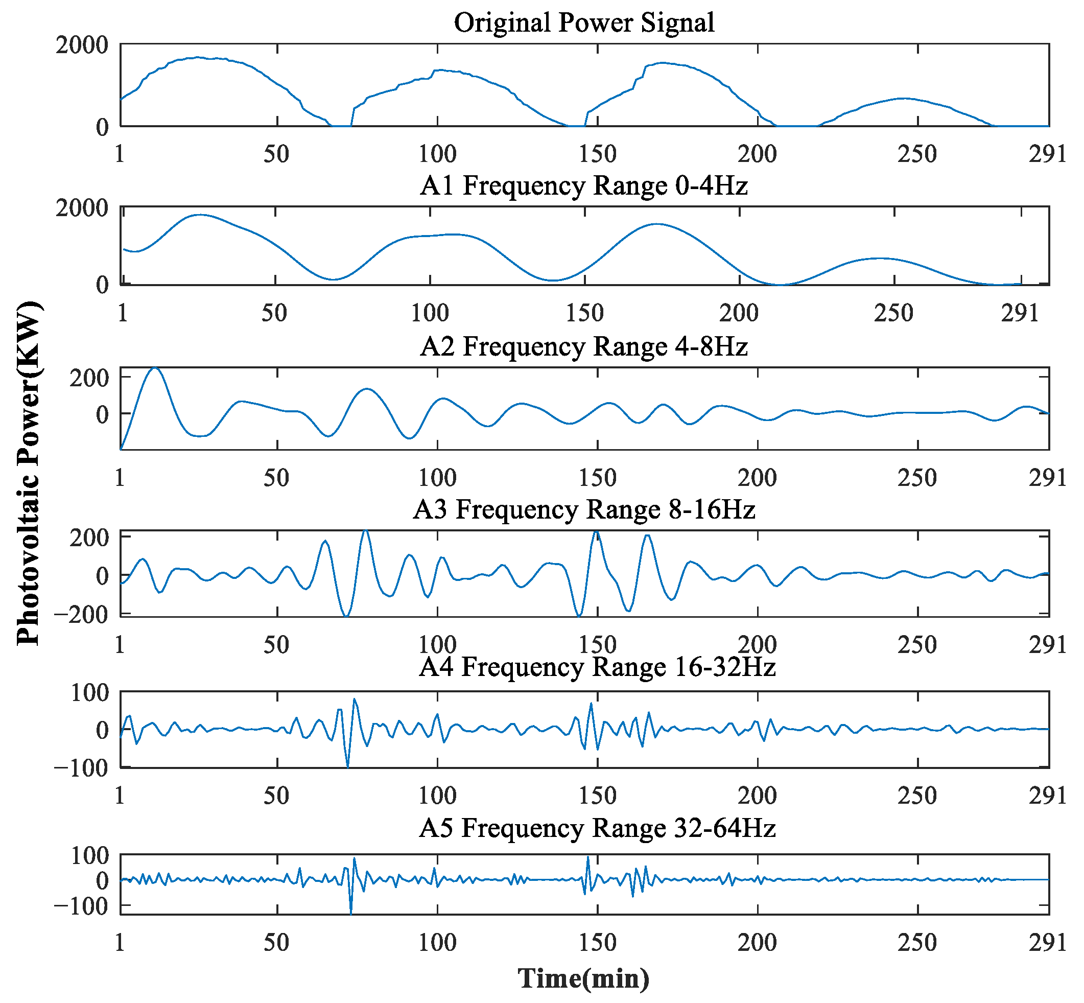
Figure 1. WT of photovoltaic power data.
Sustainability 15 06538 g001
Figure 2. Structure of CNN.
Sustainability 15 06538 g002
Figure 3. BiLSTM network model structure.
Sustainability 15 06538 g003
Figure 4. Model structure of attention mechanism.
Sustainability 15 06538 g004
Figure 5. Construction process of CNN-BiLSTM-AM model.
Sustainability 15 06538 g005
Figure 8. PPF for different training datasets and weather conditions in spring; (a) PPF on 29 April, spring (sunny); (b) PPF on 14 April, spring (cloudy); (c) PPF on 2 April, spring (overcast); (d) PPF on 19 April in spring (rainy).
Sustainability 15 06538 g008aSustainability 15 06538 g008b
Figure 9. PPF for different training datasets and weather conditions in autumn; (a) PPF on 12 October, autumn (sunny); (b) PPF on 9 October, autumn (cloudy); (c) PPF on 3 October, autumn (overcast); (d) PPF on 22 October in autumn (rainy).
Sustainability 15 06538 g009aSustainability 15 06538 g009b
Figure 10. Comparison of model forecasting accuracy under different weather conditions in spring; (a) Forecasting results for each model on 29 April, spring (sunny); (b) Forecasting results for each model on 14 April, spring (cloudy); (c) Forecasting results for each model on 2 April, spring (overcast); (d) Forecasting results for each model on 19 April, spring (rainy).
Sustainability 15 06538 g010aSustainability 15 06538 g010b
Figure 11. Comparison of model forecasting accuracy under different weather conditions in autumn; (a) Forecasting results for each model on 12 October, autumn (sunny); (b) Forecasting results for each model on 9 October, autumn (cloudy); (c) Forecasting results for each model on 3 October, autumn (overcast); (d) Forecasting results for each model on 22 October, autumn (rainy).
Sustainability 15 06538 g011aSustainability 15 06538 g011b
Figure 12. Probability density distribution of PPF errors under different weather conditions in spring; (a) Probability density distribution of PPF errors on 29 April, spring (sunny); (b) Probability density distribution of PPF errors on 14 April, spring (cloudy); (c) Probability density distribution of PPF errors on 2 April, spring (overcast); (d) Probability density distribution of PPF errors on 19 April, spring (rain).
Sustainability 15 06538 g012aSustainability 15 06538 g012b
Figure 13. Confidence intervals of PPF under different weather conditions in spring; (a) Confidence interval of the PPF on 29 April, spring (sunny); (b) Confidence interval of the PPF on 14 April, spring (cloudy); (c) Confidence interval of PPF on 2 April, spring (overcast); (d) Confidence interval of PPF on 19 April in spring (rainy).
Sustainability 15 06538 g013aSustainability 15 06538 g013b
Table 2. Forecasting average error for each training set.
SeasonError TypeMonthly Training SetSeasonal Training SetAnnual Training Set
SpringPMAE2.61%1.94%3.21%
PRMSE3.44%2.73%4.21%
SummerPMAE2.91%1.44%3.56%
PRMSE4.02%1.93%4.91%
AutumnPMAE1.92%1.07%2.37%
PRMSE2.58%1.50%3.31%
WinterPMAE1.43%0.81%1.71%
PRMSE1.81%1.08%2.32%
Error
average
PMAE2.22%1.32%2.71%
PRMSE2.96%1.81%3.67%
Table 3. Mean forecasting error for each forecasting model.
SeasonError TypeWT-CNN-
BiLSTM-AM
CNN-
BiLSTM
WT-CNN-
BiLSTM
LSTMGRUPSO-BP
SpringPMAE1.94%3.56%3.11%3.70%3.55%4.54%
PRMSE2.73%4.32%4.06%4.73%4.56%5.55%
SummerPMAE1.44%4.23%3.93%4.47%4.42%5.19%
PRMSE1.93%5.63%5.51%6.2%5.93%6.79%
AutumnPMAE1.07%2.76%2.73%2.97%2.88%3.91%
PRMSE1.50%3.35%3.62%4.13%4.08%4.54%
WinterPMAE1.53%2.13%1.88%2.45%2.53%3.58%
PRMSE2.24%2.94%2.95%3.24%3.21%4.01%
Error
average
PMAE1.32%3.17%2.91%3.40%3.34%4.30%
PRMSE1.81%4.06%3.91%4.56%4.44%5.22%
Table 4. Coverage of the confidence intervals.
SeasonDateConfidence Level
97.5%95%90%85%
Spring4.29100%100%93.15%90.41%
4.14100%100%98.59%94.36%
4.2100%96.92%96.92%95.38%
4.19100%100%100%100%
Summer8.13100%100%100%100%
8.16100%100%100%97.22%
8.17100%100%97.26%94.52%
8.5100%100%100%100%
Autumn10.1298.61%97.22%90.27%84.72%
10.9100%100%98.61%97.22%
10.3100%100%100%95.77%
10.22100%100%100%100%
Winter12.17100%100%100%100%
12.15100%97.22%90.27%86.11%
12.8100%100%100%94.20%
12.21100%100%100%100%
Disclaimer/Publisher’s Note: The statements, opinions and data contained in all publications are solely those of the individual author(s) and contributor(s) and not of MDPI and/or the editor(s). MDPI and/or the editor(s) disclaim responsibility for any injury to people or property resulting from any ideas, methods, instructions or products referred to in the content.