Groundwater Modeling to Assess Climate Change Impacts and Sustainability in the Tana Basin, Upper Blue Nile, Ethiopia

Abstract

Climate change effects on long-term groundwater (GW) resource developments in the Tana Basin, Ethiopia, are a growing concern. Efforts to provide estimates under various climatic uncertainties are lacking in the region. To address this need, we deployed a fine-resolution (500 m) GW model using MODFLOW-NWT for the Tana Basin, Upper the Blue Nile region. The GW model was calibrated based on 98 historical instantaneous well-level measurements (RMSE = 16.36 m, 1.6% of range), and 38 years of monthly lake level data (RMSE = 0.2 m, 6.7% of range). We used the model to simulate long-term climate change impacts by considering two representative concentration pathways, (RCPs) 4.5 and 8.5, from the two extreme global circulation models (MIROC5 for wetter conditions and CSIRO-Mk3 for drier conditions) available in the region. While the MIROC5 simulated GW table (GWT) was found to be stable, the CSIRO-Mk3 simulated GWT exhibited large fluctuations within +2 m to −4 m by 2100 due to climate change. More critical impacts were predicted for the lake, where total lake releases from the baseline scenario were foreseen to be changed by +50% (MIROC5) or −22% (CSIRO-Mk3) by the end of 2100.

1. Introduction

Climate change is a prominent environmental issue in Africa where effects on hydrological extremes, droughts, crop production, and groundwater (GW) resources are projected [1,2,3]. Almost 50% of the population that relies on GW are projected as being exposed to climate vulnerability [2]. In Ethiopia, climate change in combination with growing water/food and anthropogenic stresses may impose a substantial risk to its rich reserves of GW resources [4], straining the country’s sustainable development needs [5]. The country’s climate vulnerability is critical due to its rainfed irrigation dependency, severe agricultural drought, unsustainable use of resources, and existing water/food security issues [6,7]. Climate variability could affect the GW system’s direct replenishment through recharge and future GW use patterns needed to sustain domestic, industrial, and agricultural needs [8].

Ethiopia’s water resources, with a documented availability of 120 km³ for surface water (SW) and a recharge of over 36 km³ for GW [9,10], have the capacity to buffer such climatic vulnerability [11] and foster a sustainable environment [12]. The Blue Nile Basin (BNB), also known as the Abay Basin, results in more than 80% of the flows occurring during the wet season (June–September, JJAS), with seasonal variabilities. The dependence on GW during the dry season in the basin of Lake Tana (Tana Basin), the source of the BNB, is increasing [13]. Strong interannual variability and climate change may further affect the dry season flow [14], emphasizing the potential of GW to withstand future water-scarcity challenges. Despite these understandings, limited knowledge of GW sustainability, especially under an uncertain climate, affects decision-makers’ efforts to design sustainable solutions.

Driven by these motivations, we simulated the long-term impacts of climate change on the GW resources of the Tana Basin as well as several key components of the SW-GW budget in Lake Tana itself, using a calibrated GW model (referred frequently as the ‘Tana GW model’). The work builds on our previous GW modeling efforts [15,16]. By using the MODular 3-D finite-difference GW FLOW model with NWT solver (MODFLOW-NWT) [17] and the Lake Package (LAK) [18], this work attempts to complement other subsurface hydrological models in the BNB region [19,20,21,22] in overcoming the limitations of effectively simulating GW-SW interactions of Lake Tana.

Studying climate change impacts on the variability of GW levels with MODFLOW has gained some interest recently. Many studies have focused on the impacts on surface hydrological processes [23,24,25] as well as agricultural droughts [2]. Tigabu et al. (2021) [26] carried out the first attempt to use subsurface modeling to simulate climate change impacts on GW resources in the Tana Basin. However, the study only simulates the shallow GW contribution to streamflow (e.g., baseflow) in two Tana sub-basins (Gilgel-Abay and Gumera) and does not provide enough vertical details to effectively address the complex lake-aquifer interactions.

Our study is an effort to conduct physically-based GW model simulations to investigate combined climate change effects on the depth of the GW table (GWT), lake levels and the GW-SW interactions of Lake Tana. The outcome of this research may contribute to Ethiopia’s efforts to address the global challenge of sustainable development amidst climatic uncertainties [27]. Furthermore, this research seeks to provide valuable hydro-climatological information to the climate science community interested in the Upper Blue Nile region, specifically focusing on the subsurface impacts of climate change, which is a highlighted drawback in climate science [28].

2. Methodology and Data

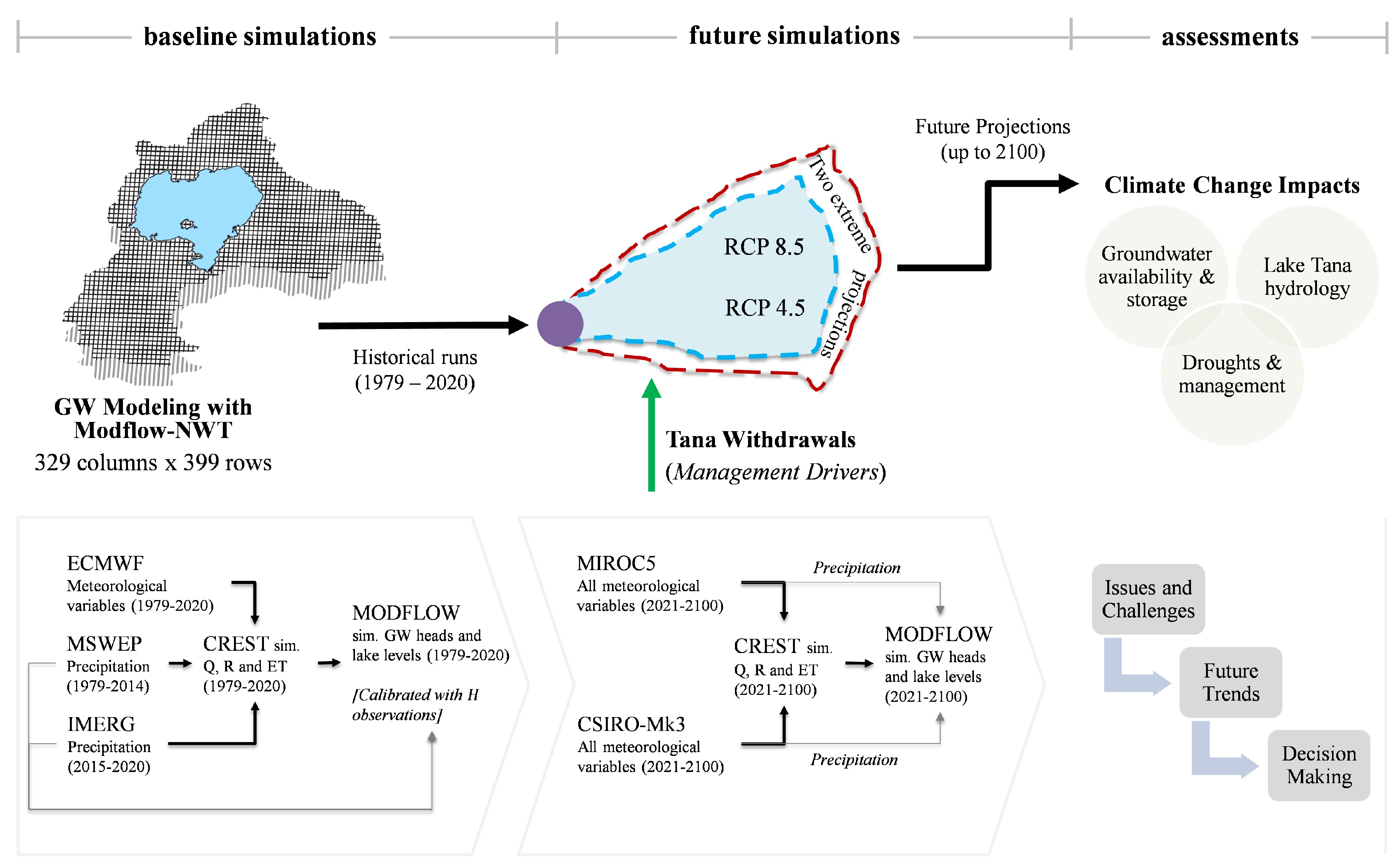
2.1. Research Framework

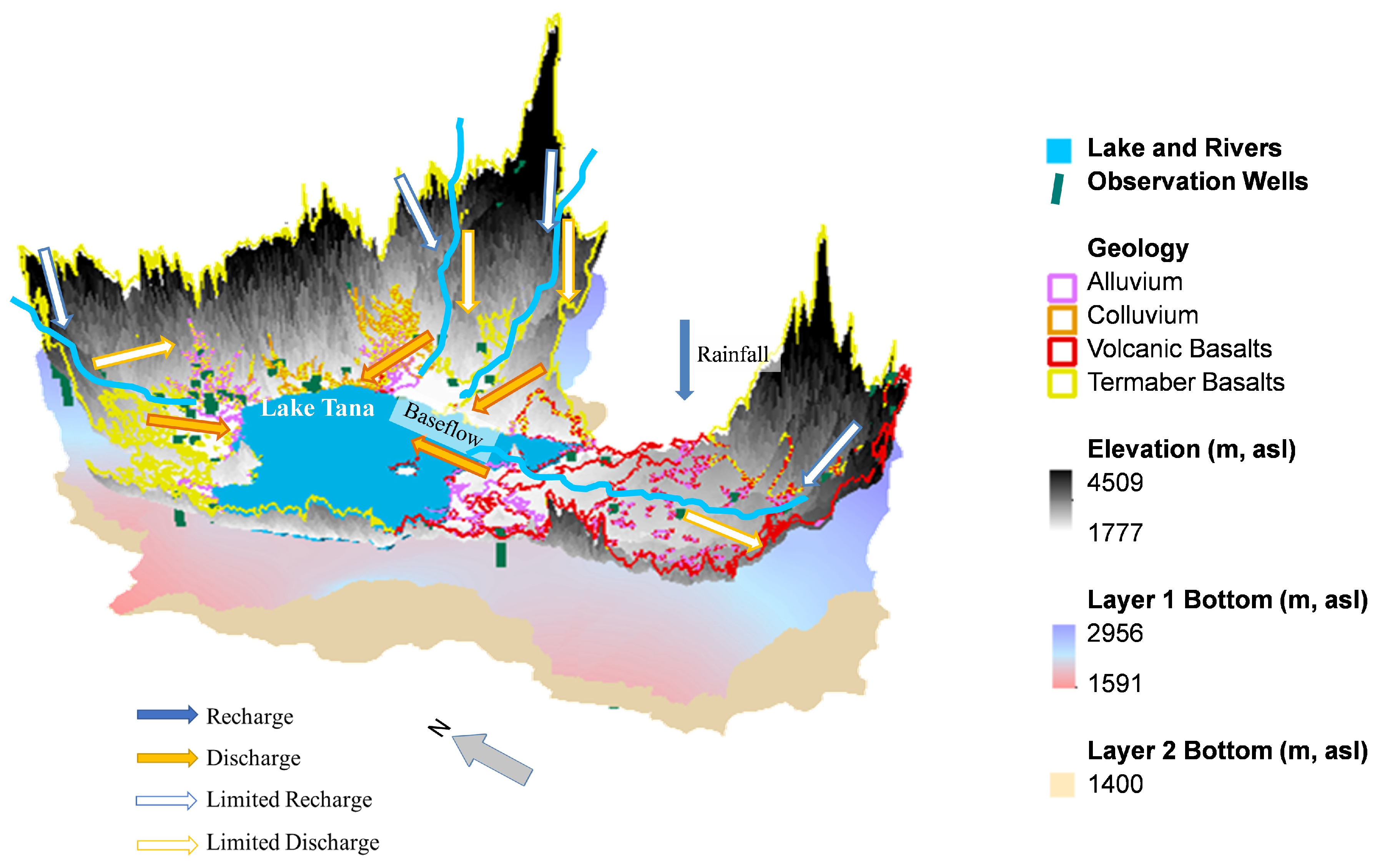
The physically based simulations of this research imply an integrated modeling approach that takes the recharge, streamflow, and lake evaporation outputs from the Coupled Routing and Excess STorage (CREST) hydrological model simulations [29] and develops a fine-resolution (500 m) calibrated GW model for a spatial domain encompassing the Tana Basin. Other key inputs to the model are overland precipitation and evaporation, which come from satellite, reanalysis, and CREST simulations, respectively. The model was calibrated with 98 instantaneous observation wells from 2013–2017, spread across the Tana Basin.

Following the baseline scenario of simulations, we used the calibrated Tana GW model to perform long-term simulations up to 2100. We used two climate change scenarios for the two general circulation models (GCMs), e.g., RCP 4.5 and RCP 8.5 to pass the meteorological forcings to CREST. We then simulated recharge, streamflow, and lake evaporation using CREST, which were added as inputs to the calibrated Tana GW model. More details on CREST and GCM data processing are available in [29,30] and are beyond the scope of this research.

Figure 1 is a process diagram showing the key components of this research. The Tana withdrawals (Figure 1) mostly accounted for irrigation, hydropower, and domestic withdrawals. We used climate change simulations to investigate the long-term physical availability of GW resources in the Tana aquifer, Lake Tana level variabilities, and potential GW depletions. We also simulated the subsurface water budget components to map key lake-aquifer interactions.

2.2. Study Area

The model domain encompasses the Tana Basin (latitudes of 10.95° N to 12.50° N and longitudes of 36.73° E to 38.20° E, and covers an area of 15,096 km²) shown in Figure 2. Figure 2 also shows the Tana sub-basins, tectonic faults, and the 98 historical wells used in model calibration. The Tana Basin topography varies from about 4509 m on the east to around 1777 m near Lake Tana. Several irrigation schemes have been proposed within the Tana Basin in the past decade. Environmental flow from the lake is primarily released through the Blue Nile outlet (Figure 2). Lake Tana is the largest lake in Ethiopia, accounting for 50% of the freshwater resources for the country, including water for domestic use, irrigation, hydropower production, fisheries, grazing, and livestock. Hydropower withdrawals largely account for the requirements of the Tana Beles project established in 2010 [31]. The Tana Beles project, together with existing national plans [32], offers hope for energy transition in the region. Lake Tana and its adjacent wetlands provide a livelihood to more than half a million people [33], including the Negede people whose livelihood depend on making boats and baskets from papyrus. Lake Tana is an important source of fish for communities around the lake and beyond, while the lake wetlands are very important for breeding and enhancing biodiversity, sediment retention, and flood protection [34]. The lake is also a popular tourist destination, offering many opportunities for recreational activities to its visitors. The region’s tourism and ecological value played a key role in UNESCO’s inclusion of the Lake Tana biosphere reserve [32].

2.3. Data Description

The research utilizes the one-way coupling of MODFLOW with CREST, and in the process, uses the following three tiers of data:

• Static features—topography, geology, river network, and fault lines, collected primarily from the 90 m DEM [35] and from Kebede (2012) [10].
• Dynamic forcings—lake precipitation datasets from a combination of satellite precipitation and atmospheric reanalysis, e.g., MSWEP [36], IMERG [37], and ECMWF [38]; climate model simulations, e.g., MIROC5 [39] and CSIRO-Mk3 [40]; CREST simulated streamflow, recharge, and lake evaporation—driven by the above precipitation and climate scenarios.
• Secondary datasets—historical data on 98 GW wells, borehole information, lake levels (1979–2017) measured near the Blue Nile outlet (Figure 2), lake outflow, and Koga reservoir levels (2012–2019) received from different line agencies—i.e., the Abay Basin Authority (ABA), Bahir Dar University (BU), and the Ministry of Water, Irrigation, and Energy—Ethiopia.

One-way model coupling was carried out with daily recharge ($R$), streamflow ($Q$), and lake evaporation ($E$) simulated by CREST. The LAK package requires inputs on anthropogenic water withdrawals ($W$). Given the management uncertainties and lack of accurate information, we adjusted values of $W$ during calibration, with constraints obtained by a thorough review of the existing literature [31,41].

We used the climate projections from a Regional Climate Model (RCM), named Rossby Centre Atmospheric Model version 4 (RCA4) for representative concentration pathways (RCP); 4.5 and 8.5 (All RCA4 downscaled GCM data were downloaded from https://esgf-node.llnl.gov/search/esgf-llnl/, accessed on 11 January 2022). RCPs are concentration pathways, which are characterized by the radiative forcing to be produced by the end of the 21st century [28]. The RCA4 provides an ensemble of future climate change scenarios [42]. In this RCM, the variables (precipitation, temperature, radiations, humidity, air pressure, and wind speed) are downscaled to 3 hourly and 50 km resolution from different general circulation models (GCMs) of the Coupled Model Intercomparison Project 5 (CMIP5) [43]. Since we aimed to analyze the impact of future extremes, we selected the wettest and driest GCMs from all available downscaled GCM products in the RCA4 model, using the annual precipitation change against the baseline (1976–2005) as the criteria. As Figure 3 shows, the Model for Interdisciplinary Research on Climate (MIROC5) [39] projects the wettest precipitation trend in all three future time windows, early-century (2011–2040), mid-century (2041–2070), and late-century (2071–2100); whereas CSIRO [40] indicates the driest condition. First, CREST-SVAS was calibrated using the historical baseline period (1981–2005) and the downscaled forcing variables from these two GCMs. Then, calibrated parameters were used in future simulations with MIROC5 and CSIRO projections. CREST-SVAS simulated outputs (streamflow, infiltrations, and potential evapotranspiration) for the wettest and driest climate scenarios were then used as inputs to the MODFLOW groundwater model.

Figure 3 shows the precipitation anomalies for different climate change scenarios compared to the baseline (1981–2010) precipitation of the corresponding GCM in the Upper Blue Nile Basin area (Figure 3a). The figure also shows annual precipitation trends for the wettest (MIROC5) and driest (CSIRO) GCMs used in our study. Figure 3b further highlights how the selection of dry and wet projections continues to incorporate precipitation uncertainties (one of our primary forcings) in our long-term modeling work.

2.4. Groundwater Modeling

The groundwater modeling performed in this research was built on our previous research in the Gilgel-Abay sub-basin [15]. In this work, we modified the previous model by spatially extending it to encompass the entire Tana Basin and simulating the water levels and lake-aquifer interactions in Lake Tana, using MODFLOW’s Lake Package (LAK) [18]. The conceptual model was developed using information from the previous literature [44] in combination with the conceptual model built in our previous work [15] and is shown in Figure 4. The stratigraphic assembly, primarily developed by Hautot et al. (2006) [44], comprises a sedimentary basin of about 1.5–2 km thick beneath the basaltic lava flow, which spreads as deep as 250 m in some areas (Figure 4). As such, the numerical model MODFLOW-NWT included two vertical layers (aquifers). The distributed thickness of the top layer was obtained by performing a Kriging interpolation [45] on borehole depth records of the 98 observation wells. During the simulation, the bottom aquifer was always confined, and the top aquifer was unconfined (both were specified as ‘convertible’ in the model).

The GW model was calibrated using a trial-and-error–based approach to minimize the root mean squared error ($RMSE$) between simulated and observed heads, from the 98 historical wells. Hydraulic conductivity ($K$), specific yield ($S_y$), unit streambed conductance ($\zeta$), recharge-infiltration ratio (${\varphi }_{R/I}$), and lakebed leakance ($lk$) were considered as major calibration parameters based on the literature [13]. Among these, $K$, $\zeta$ and $S_y$ are spatially distributed, whereas ${\Phi }_{R/I}$ and $lk$ is spatiotemporally constant. In addition, we also adjusted some other parameters during calibration, i.e., specific storage ($S_s$) and boundary flux ($q$). Initial values of these calibration parameters were selected based on the literature [10,46,47]. We also evaluated the calibrated GW model by forcing it with past data (precipitation) and resulting CREST simulations ($Q$, $R$, and $E$) from the two climate projections, MIROC5 and CSIRO-Mk3. The past climate forcings from 1980 to 2020 used in this evaluation encompassed a combination of bias-corrected available (1980–2006) historical climate data and bias-corrected RCP 4.5 climate change projections (2007–2020).

2.5. Future Scenarios

Climate change simulations were conducted under the same setting as the baseline scenario, which we defined in this study from the period of 1991–2020 (allowing 10 years of model warm-up period). In the IPCC 5th Assessment Report (AR5), climate change scenarios were defined based on total anthropogenic radiative forcings by the end of the 21st century [28]. The RCPs represent different concentration paths of climate change scenarios, and in this study, we selected RCP 8.5 (high emission: 8.5 Wm⁻²) and RCP 4.5 (stabilized emission: 4.5 Wm⁻²) together to have a better understanding of the uncertain climate up to 2100. It is also a common practice in hydrological modeling research to consider these two RCPs [48,49,50].

In order to specify the lake releases for future simulations, we used varying withdrawals, $W$ (adjusted during calibration) within the threshold of 3 km³ maximum withdrawal accounting for the Tana-Beles hydropower project [31]. For future simulations, we used the same $W$ as the calibrated estimate during Tana Beles operations (2009–2020). We let MODFLOW simulate lake outflow ($Q_o$) at the Blue Nile outlet, based on the water available in the lake, after specifying thresholds of lake level fluctuations. This allowed us to incorporate sufficient variability in future total lake releases, which was an improved consideration than just assuming different scenarios of lake releases, which would be computationally expensive as well.

2.6. Climate Change Impacts

Following the long-term simulations, we investigated a range of potential impacts of climate change on the (a) physical availability of GW resources in the Tana Aquifer, (b) hydrology of Lake Tana, and (c) future GW level fluctuations and resource management. While assessing these impacts, we focused on specific issues and challenges encountered by the simulations, explored the future trends, and investigated how such trends might relate to future water management decision-making in the Tana area.

The analyses were temporally conducted in four different time periods from the GW modeling standpoint, e.g., a baseline (1991–2020), early-century (2021–2050), mid-century (2051–2080), and late-century (2081–2100). Aside from investigating time-series estimates of lake levels and spatiotemporal estimates of GW head ($H$), we also assessed GW depletions and future lake and reservoir management at regional and local scales.

We used the standardized water level index (SWI) defined by Bhuiyan (2004) [51]. This index is a simplistic approach to estimating GW depletions that includes estimating the normalized differences (with respect to standard deviation) of GW levels from the baseline mean (where $+ve$ values indicate a drop in water levels). The method is considered for its generalizability in different parts of the world [52,53], and more specifically, in Ethiopia [54]. SWI values within 0–1 are classified as mild depletion, while values from 1–2.5 refer to moderate, 2.5–4 refer to severe, and >4 refer to extreme GW depletions. For the lake, we did not estimate any water-level-based drought indices, as the calibrated GW model was not forced with enough data to provide accurate estimates of lake levels corresponding to the complex management effects through operations of existing water control and regulatory structures. Instead of lake levels, we analyzed the total lake releases, which is a combination of withdrawals, $W$, and lake outflow, $Q_o$, to obtain an understanding of future trends and impacts on lake and reservoir management at regional and local scales.

3. Results

3.1. GW Model Evaluation

This section presents the summary of the model calibration parameters, how the simulated surface and groundwater levels compare against historical observations, and how the calibrated GW model performed with historical climate forcings.

3.1.1. Calibrated Parameters

Figure 5a shows the calibrated values of $K$, and $q$. In addition, Figure 5b shows the annual average recharge, which was calibrated as 30% (${\Phi }_{R/I}$) of the infiltration simulated by CREST. The calibrated $K$ values entailed a wide range of values in different geological regions (shown in Figure 5). For most of the basaltic regions in the top aquifer, $K$ values were low (0.1~0.5 m/d), while at alluvial formations, it was significantly higher. This is also in accordance with the literature [10,46,47,55,56,57]. The calibrated $S_y$ distributed from 0.05~0.2 in the top unconfined aquifer had similar variability as $K$ (

Table 1. Summary of model calibration parameters.

Parameter	Aquifer	Initial Values	Calibrated Values
$K$	Top	Horizontal: 1 m/d	Horizontal: 0.1–40 m/d
		Vertical: 0.1 m/d	Vertical: 0.01–4 m/d (i.e., 1/10th of Horizontal K)
	Bottom	Horizontal: 0.5 m/d	Horizontal: 0.5 m/d or equal to Top Aquifer’s horizontal K (whichever is less)
		Vertical: 0.05 m/d	Vertical: 0.05 m/d or equal to Top Aquifer’s vertical K (whichever is less)
$S_y$		0.05	0.05 (for $0.1\le K<10$), 0.1 (for $10\le K<20$), 0.15 (for $20\le K<30$), and 0.2 (for $K\ge 30$)
$\zeta$		0.1 m/d	0.05~1 d−1
${\Phi }_{R/I}$		10%	30% of CREST infiltration
$S_s$		10−4 m−1	10−6 m−1
$q$		from contour map of [60]	1~2 m/d during dry season, 2~5 m/d during wet season
$lk$		0.5 d−1	1 d−1
$W$		1 km3	0.6 km3 (1979–2000), 0.75 km3 (2000–2008), 1.26 km3 (2008–2020)

). For the bottom aquifer, calibrated $S_s$ was found as 10⁻⁶ m⁻¹. The calibrated $S_y$ was also reasonable in comparison to the literature [46,58]. The calibrated values for $\zeta$ were obtained as 1 d⁻¹ for the four major rivers, Gilgel-Abay, Megech, Ribb, and Gumera, and 0.05 d⁻¹ for all other minor rivers. The calibrated value of ${\Phi }_{R/I}$ = 30% indicated 30% of net infiltration was used as recharge and was also supported by the recent literature [59]. Moreover, calibrated flux ($q$) was 1~2 m/d during the dry season and 2~5 m/d during the wet season. The lakebed leakance, $lk$, was calibrated as 1 d⁻¹. The lake withdrawals ($W$) increased over time and were also adjusted during model calibration (varying from 0.6 to 1.26 km³). From 2008–2020, higher $W$ values were assigned to represent the Tana Beles water withdrawals during the project operation phase. Table 1 summarizes calibrated model parameters, and Figure 5 shows the spatial distribution of horizontal $K$ values for the top aquifer (with $K_x$ = $K_y$) and $q$ values.

3.1.2. Model Calibration

The calibration results are shown in Figure 6. Figure 6a indicates a good agreement ($RMSE$ = 16.36 m, R² = 0.99 and p < 0.0001) of simulated heads with 98 observations (instantaneous data for 2013–2017). Figure 6a also highlights the spatial bias distribution (red: overestimation, blue: underestimation). The bias is consistently spread across the model domain and despite some high errors in groundwater head predictions, it does well in capturing a large range of observations (1017 m, with a normalized RMSE of 1.6%).

Figure 6b shows the model calibration results against monthly observed water levels in Lake Tana from 1979 to 2017. The result shows that the groundwater model, taking advantage of the lake-aquifer interactions incorporated by the sophisticated lake package module of MODFLOW, was able to capture the trends and seasonality of the lake level dynamics, with an RMSE of 0.2 m (R² of 0.89 and p < 0.05). In general, the simulated lake levels had a slightly lower variability in comparison with observations, but the mean water levels were in good agreement.

3.1.3. Performance with Historical Climate Forcings

Upon testing the calibrated GW model with historical (1980–2006) and projected (2006–2020) climate datasets and comparing the simulated $H$ values with the same set of 98 instantaneous observation wells, we obtained an RMSE of 16.98 m for MIROC5 forcings and 16.72 m for CSIRO-Mk3 forcings (Figure 7). These values were similar to the RMSE obtained for the actual calibrated model solely forced with CREST simulations driven by ECMWF and MSWEP/IMERG reanalysis datasets. It is to be noted that despite the RMSEs being similar to the CREST-calibrated model, the spatial distributions of biases with observed $H$ are not identical in either of the models presented in Figure 6a and Figure 7a,b.

3.2. Spatiotemporal Water Availability and Climate Change Impacts

This section explores the long-term impacts of climate change in the GW levels simulated across the model domain as well as the long-term changes in water levels of Lake Tana. Results are presented on how the future climate might impact regional water availability by considering both the wettest and driest climate models.

3.2.1. Groundwater Table

The climate change impacts on the GW table (GWT) in the model domain are shown below in Figure 8. The average depth of GWT for the baseline period (1990–2020) is shown in Figure 8a. The figure shows relatively shallow (within a depth of 5 m from the surface, marked by a blue color) groundwater availability along the major river routes in the Tana Basin. There are some regions where the GWT drops to moderate depths of up to 30 m. In some areas, e.g., areas with high elevations in the south and east, the areas within the northern flood plains, and the Megech sub-basin regions, some deep GW areas are encountered where the water table dropped approximately 40~50 m. The majority of the lowest GW areas were found in areas where the model domain was intersected by the specified hydrogeological boundary conditions (no-flow boundaries, specified flux, intersections of faults and rivers, etc.). The figure also shows a contour map of simulated hydraulic heads, $H$, for the baseline simulation period (Figure 8d). This showcases the direction of GW flow within the aquifer (towards Lake Tana).

In Figure 8(b1,c1), we compared the long-term simulated GW levels, primarily forced with the two projections (RCP 4.5 and RCP 8.5) of the wettest (MIROC5) and driest (CSIRO-Mk3) climate models. The figures represent the temporally averaged anomalies of GW levels for three different 30-year spans up to 2100 (2020–2050, 2051–2080, and 2081–2100), in comparison with the baseline GW levels shown in Figure 8a. The blue and red shades in Figure 8(b1,c1) represent water gains and losses, respectively. In addition, Figure 8(b2,c2) provide boxplots to showcase the spread of individual data points used to prepare the temporally averaged maps in Figure 8(b1,c1). The boxplots presented in Figure 8, as well as all subsequent figures, showcase the 5% and 95% quantiles by the transect lines in the extreme ends, whereas the 25% and 75% quantiles are marked by the solid rectangles.

From the baseline scenario, the MIROC5 RCP 4.5 simulated mean GWT changed by +0.05 m (2021–2050), +0.1 m (2051–2080), and +0.02 m (2081–2100); whereas the MIROC5 RCP 8.5 simulated mean GWT changed by +0.11 m (2021–2050), +0.09 m (2051–2080), and +0.1 m (2081–2100). From CSIRO-Mk3 projections, RCP 4.5 simulated mean GWT changed by +0.01 m (2021–2050), −0.35 m (2051–2080) and −0.6 m (2081–2100); whereas the MIROC5 RCP 8.5 simulated mean GWT changed by −0.01 m (2021–2050), −0.4 m (2051–2080), and −0.8 m (2081–2100).

3.2.2. Lake Tana Dynamics

The lake inflows ($Q_i$, accounting for both SW and GW contributions) and outflows ($Q_o$ through the Blue Nile outlet releases, GW outflow, plus the withdrawal, $W$) for the baseline scenario (1991–2020) was simulated by the Tana GW model as 1675 mm/yr and 1666 mm/yr, respectively. Sequentially, to investigate the climate change effects on future water levels and releases of Lake Tana, we simulated our calibrated GW model up to 2100 under the four different projections (e.g., RCP 4.5 and RCP 8.5 for the two climate models). Figure 9 below summarizes the results, where the top two sub-plots show the time series of monthly lake levels, and the bottom sub-plot shows the time series for annual lake releases. The relaxation of Tana outflow through the Blue Nile outlet led to peak water levels being fixed at 1787 m for most of the years, except when instances of dry years could be foreseen, and the lake level was not able to revive into normal conditions due to releases being too high (Figure 9b).

The MIROC5 RCP 4.5 model projections revealed a few dry spells (Figure 9(a1)), most notably the one in the early 2080s when the water level was simulated to be below 1785 m. For the dry model CSIRO-Mk3, there was one notable dry spell encountered in the mid-2050s. In 2081–2100, the dry model—with specified withdrawals equaling existing estimates and no specified releases (which were computed by the model itself)—exhibited a sustained drop in water levels (Figure 9(a2)). For the CSIRO-Mk3 RCP 4.5 scenario, the lake levels gradually replenished back to normal, but for the extreme CSIRO-Mk3 RCP 8.5 scenario, lake levels were not able to revive within the simulation time frame (up to 2100). When we compared this phenomenon with the total releases (constituting specific withdrawal and MODFLOW estimated releases), we found that there was no annual variability in total releases from 2081–2100 in the CSIRO-Mk3-forced simulations. This indicates that after sustaining the specified Tana withdrawals, there was not enough water to be released through the Blue Nile outlet, which would introduce hydrologic variabilities.

For a dry climate model such as CSIRO-Mk3 to happen in the near future, it would not be possible to have $W$ as current; therefore, we proposed a 50% reduced $W$ scenario (the ‘conservative’ scenario, suffixed with ‘b’ in Figure 9(a2,b)). With the reduced withdrawal, $W$, during the CSIRO-Mk3 scenarios, the lake levels revived back above the minimum thresholds. At the same time, more releases through the Blue Nile outlet were simulated, which is important considering the two major downstream irrigation schemes, Tis-Abay I and Tis-Abay II, which rely on the variability of lake releases [10,31].

3.3. Subsurface Water Budget and Climate Forcings

We compared different simulated sub-surface water budget components with the three primary model forcings, precipitation ($P$), evaporation ($E$), and recharge ($R$), for both the baseline and future scenarios, shown in Figure 10 (all estimates are in mm/d). The mean annual precipitation and evaporation used in the Tana GW model were 1319 mm/yr and 1392 mm/yr respectively. The GW contributions towards the annually averaged baseline lake inflows ($Q_i$) of 1675 mm/yr was 15%, which is 8% of the total lake inflows (including $P$). For lake outflows, we estimated a total annually averaged release of 1666 mm/yr, of which the Tana withdrawals ($W$) accounted for 15% during 1991–2008 and 26% during 2009–2020.

Figure 10 shows boxplots of annually averaged estimates, of which precipitation and evaporation are over the lake, while all other water cycle variables (recharge, seepage into the lake, baseflow, and drainage through faults) are for the entire model domain (Tana Basin). The future precipitation scenarios offer a more extreme variability compared to the baseline. However, the median estimates for the climate model scenarios are slightly lower than the baseline. In general, precipitation from MIROC5 was higher than CSIRO-Mk3. For evaporation, the projected variabilities were similar to the baseline, with median values gradually increasing across the three different timelines, e.g., 2021–2050, 2051–2080, and 2081–2100. Of all other input forcings, recharge values exhibited substantial variability, and for the CSIRO-Mk3 RCP 8.5 scenario, which was the driest of all, recharge values were significantly less for the 2021–2050 and 2081–2100 time periods.

3.4. Future Impacts and Water Management

3.4.1. GW Depletion

Upon analyzing the monthly GW level simulations for future climate events, we did not find any ‘moderate’ or worse GW depletions (e.g., SWI > 1) when compared with the baseline scenario (1991–2020). As such, Figure 11 only shows the number of months in a year when each model grid was predicted to be subjected to ‘mild’ depletion. Areas of mild depletion exhibited in MIROC5 RCP 4.5 simulations were 20% (2021–2050), 18% (2051–2080), and 22% (2081–2100); whereas the MIROC5 RCP 8.5 simulated estimates were 17% (2021–2050), 18% (2051–2080), and 16% (2081–2100). In contrast, areas of mild depletions for CSIRO-Mk3 RCP 4.5 simulations were 17% (2021–2050), 32% (2051–2080), and 48% (2081–2100); whereas the CSIRO-Mk3 RCP 8.5 simulated estimates were 21% (2021–2050), 46% (2051–2080), and 68% (2081–2100). To summarize, for the dry climate scenarios (CSIRO-MK3 RCPs 4.5 and 8.5), a significant portion of the areas were found to experience mild depletions in the future. For the wet scenarios (MIROC5 RCPs 4.5 and 8.5), there were some areas along the southeast boundaries in the Gilgel-Abay sub-basin, and significant areas from Ribb and Gumera sub-basins that were found to experience mild depletions.

3.4.2. Surface Water Availability and Management

We also investigated the surface water availability in Lake Tana by exploring the future simulated releases already presented in Figure 9b. In this analysis, we did not compute any water-level-based indices as we did not use our model to simulate the dynamic lake levels corresponding to the complex management effects through operations of existing water control and regulatory structures. Rather, as our model was used to primarily estimate lake releases through the Blue Nile outlet, supported by the imposed water budget constraints and the relaxation of the simulated lake levels between specified thresholds, we compared the total releases against the baseline (Figure 12).

For MIROC5 RCPs 4.5 and 8.5, our simulations predict a substantial increase in mean annual releases of about 3 km³/yr (more than 50% from baseline mean) from Lake Tana during the later part of the century, while sustaining peak lake levels of 1787 masl. In contrast, using the CSIRO-Mk3 RCPs 4.5 and 8.5 scenarios, our simulations show a drop in mean annual releases, which could be as much as 1.2 km³/yr (22% of baseline mean) for the most extreme case of CSIRO-Mk3 RCP 8.5. This indicates that total releases from Lake Tana could undergo significant changes to account for the growing needs amidst uncertainty with climate change.

To investigate the effects of climate change on local-scale reservoir operations and irrigation management, we used the calibrated GW model to predict water levels in Koga Reservoir, Ethiopia (shown in Figure 2), which is the largest reservoir-operated irrigation scheme in the Tana Basin with approximately 7000 ha of coverage [61]. Figure 13a shows the long-term simulated reservoir levels. In order to represent the local reservoir in our model domain, we used a simple technique called “high K” [18], where the cells representing the Koga reservoir were specified with a high hydraulic conductivity (can be seen in the spatial distribution of calibrated $K$ in Figure 5). A high specific yield was also assigned for the top layer. The simulated reservoir levels were calibrated with 2012–2019 observed levels (RMSE of 0.7 m, R² = 0.863, and p < 0.05), and the results are shown in Figure 13b.

4. Discussion and Study Limitations

The study underscores the climate change effects on the future availability of GW resources in the Tana Basin as well as the future water levels and releases of Lake Tana.

Table 2. Performances of other GW models of interest.

Model [Source]	Location	Error	Calibration Data	Remarks
MODFLOW [11]	Gumera Basin (Lake Tana sub-basin)	1.7 m	One well (nine months’ records)	Known boundaries provided, extensively calibrated at one well.
MODFLOW [13]	Northern part of Tana Basin	~10 m	58 observation wells	Calibration dataset was not spatially as distributed as ours.
MODFLOW [47]	Tana Basin	~20 m	37 target wells	The spatial pattern of $K$ is similar to our study.
MODFLOW and LISFLOOD [62]	Bulgaria	~30 m	Model not calibrated with in-situ data	Highlights challenges in SW/GW model coupling.
SWAT-MODFLOW [22]	Parts of Tana Basin (Gilgel-Abay, Ribb and Gumera)	~0.45 (normalized with $SD$)	36 instantaneous wells	Aquifer interactions are not well purported by only one 6 m vertical layer.
CREST-MODFLOW [15]	Gilgel-Abay Basin	14.4 m	38 instantaneous wells	Lake Tana was not simulated and observed lake levels were rather specified as a downstream constant head boundary.

shows the performance of some other GW models reported in the Lake Tana region. Our normalized RMSE, with a range of 1017 m, was 1.6%, which is better than our previously calibrated model in the Gilgel-Abay region. Another aspect worth considering is that the Gilgel-Abay GW model was fed with specified constant boundaries of observed lake levels. In the Tana GW model, however, lake levels were independently simulated, which was again efficiently calibrated against observed time-series records (RMSE = 0.2 m). Considering the in-situ data scarcity, the regional scale, and the performances of other coupled GW models, [62,63], the results are acceptable. The model performed well in capturing the GW levels with bias-corrected climate projections, as it did for the reanalysis-based forcings. This supports our calibrated Tana GW model to simulate and capture future long-term climatic events when we force the model with MIROC5 and CSIRO-Mk3-based forcings from 2020 to 2100.

In Figure 8 (Section 3.2.1), the averaged GW level anomalies varied from +2 m to −4 m from baseline estimates. In general, more water gain was exhibited for the wet climate model, MIROC5, whereas the dry climate model, CSIRO-Mk3, led to significant water losses. Water losses for the dry climate model CSIRO-Mk3 were more prominent in high-elevation areas, e.g., east of the Ribb and Gumera sub-basins, and south of the Gilgel-Abay sub-basin. Among the two different projections, RCP 8.5 indicated more extreme water loss (for the CSIRO-Mk3 model). MIROC5 RCP 8.5 forced GW levels were found higher than MIROC5 RCP 4.5.

Figure 9 in Section 3.2.2 shows how the two extreme GCMs relate to long-term water availability in Lake Tana. Lake Tana is a lake that undergoes a wide range of controls [31,41], and our physically-based modeling, primarily considering the hydrologic sensitivities, marks an acceptable effort in simulating the lake’s behavior. From a GW modeling perspective, this was a major challenge to efficiently use MODFLOW’s LAK package to simulate the complicated lake-aquifer processes [18]. An interesting point here is how different climate change projections reveal different conditions (dry and wet) for the future. The GW model also predicted similar outcomes, with foreseeable long-term fluctuations in lake releases as +50% (MIROC5) or −22% (CSIRO-Mk3) by 2100. While this information seems overwhelming from a decision-maker’s perspective, the knowledge of future climatic uncertainties highlights the need to adopt a flexible decision-making approach to ensure sustainable development. More specifically, adaptive (considering both dry and wet scenarios) and equitable sharing of Lake Tana water resources could be mandated by designing policies for each 30-year span into the future (e.g., 2021–2050, 2050–2080, and 2080–2100). This way, the water managers and farmers would be prepared to exercise flexible ways of water sharing and use.

The lake inflows and outflows simulated by our calibrated GW model for the baseline period (1991–2020) were 1368 mm/yr, and 1667 mm/yr, respectively. For future climate simulations, we used MODFLOW’s LAK package to simulate river releases through the outlet in a way so that the lake levels vary within a specified threshold (1784 m to 1787 m, based on the existing regulatory standard), and all water budget components are balanced, accounting for the withdrawal, $W$, for hydropower and domestic purposes.

The reduced withdrawal scenarios (suffixed with a ‘b’ in Figure 9) produced a compromised outcome of lake levels. Lake Tana’s water level increased substantially in the ‘conservative’ scenario. The mean releases were the same as the ‘regular’ scenario for the CSIRO-Mk3 model projections, but this ‘conservative’ scenario added more seasonal variability in releases (Figure 9b), which would better reflect the agricultural needs of existing irrigation schemes in the Tana Basin. As we reduce the withdrawals by 50%, about 0.63 km³/yr of water could be allocated in the late-century period (2081–2100) from hydropower to agricultural needs. If a critical circumstance arises (e.g., CSIRO-Mk3 RCPs 4.5 or 8.5), this could feed a significant portion of projected agricultural water requirements of 0.93 km³ in the area [64]. This scenario would, however, compromise direct withdrawal ($W$), accounting for the hydropower requirements of the Tana Beles project, leading towards a more manageable problem.

The simulated water budget variables (shown in Figure 10, from Section 3.3), namely, seepage into the lake, baseflow, and drainage through the faults, offer more erratic shifts across the different timelines. The seepage into the lake—despite increasing and reducing in different periods compared to the baseline—was always positive, meaning that upon considering annually averaged estimates, the lake is always expected to gain net water from the aquifer GW discharge. The same could be said for both baseflow and drainage through the faults. The faults, on the other hand, offered some drainage through the saturated aquifers throughout the simulated timeline. For all these components, the dry-climate scenarios (CSIRO-Mk3 RCPs 4.5 and 8.5) simulated substantially low estimates in future.

The Tana GW model revealed a mean baseflow of 0.25 mm/d, which was 58% of the entire basin’s mean annual recharge of 158 mm/yr (spatial average of distributed recharge shown in Figure 5b). Kebede (2012) [10] reported a mean annual recharge of about 300 mm/year in the Gilgel-Abay region, which also appears to be consistent with the spatial estimates of Figure 5b. Overall, the percentage of recharge contributing to baseflow, as simulated by the Tana GW model, agreed with some other studies [65,66]. The magnitudes of drainage through faults were less, nevertheless, the fault lines’ inclusion as drains helped improve model performance (in comparison with observations).

Table 3. Annual water budget of Lake Tana from various sources [67]. Here, * gauge and empirically fitted, ** hydrological model-based (SWAT, CREST, MODFLOW, etc.), and *** satellite and reanalysis-based analysis. All values are in mm/yr.

Source	Year	$\mathit{E}$	$\mathit{P}$	${\mathit{Q}}_{\mathit{i}}$	${\mathit{Q}}_{\mathit{w}}+\mathit{W}$	$\mathit{L}$
Kebede et al. (2006) [68] *	1960–1992	1478	1451	1162	1113	22
SMEC (2008) [55] *	1960–1995	1650	1260	1622	1231	1
Gieske et al. (2008) [69] *	1992–2003	1671	1255	1770	1348	19
Wale et al. (2009) [70] **	1992–2003	1690	1220	2160	1520	170
Chebud and Melesse (2009) [20] **	1960–2003	1428	1198	1458	1679	−451
Setegn et al. (2008) [71] **	1978–2004	1248	1375	1312	1280	159
Rientjes et al. (2011) [72] ***	1994–2003	1563	1347	1781	1480	85
Tegegne et al. (2013) [73] **	1996–2002	1618	1291	2119	1725	67
Nigatu (2013) [74] *	1994–2003	2041	1274	2186	1520	−101
Duan et al. (2018) [75] ***	2006	1688	1652	2226	1566	191
Dessie et al. (2015) [76] *	2012–2013	1789	1330	2349	1618	273
Mamo et al. (2016) [77] **	1995–2005	1544	1315	2829	1552	945
Alemu et al. (2020) [67] *	1990–2007	1650	1190	1415	1124	−169
Lazin et al. (2020) [29] **	1979–2020	1392	1319	1527	1342	95
Tana GW Model **	1991–2008	1359	1269	1719 (SW 85%, GW 15%)	1698 (SW 84%, GW 0.3%, W 15%)	−69
	2009–2020	1452	1408	1608 (SW 84%, GW 16%)	1618 (SW 74%, GW 0.3%, W 26%)	−54

shows different estimations of the annual inflows and outflows of Lake Tana. About 8% of total lake inflows (from river, aquifer, and precipitation sources) were contributed by GW sources (lake seepage, shown in Figure 10). The Tana GW model exhibits an improved understanding of lake-aquifer interactions, as it simulates the GW inflows and outflows from the lake. Specification of $W$ allowed us to minimize the losses ($L$) of the lake water budget, which was a challenge for other hydrological models reporting lake releases (Table 3).

Figure 11 in Section 3.4.1 showed the likelihood of future GW depletions. The mild depletions (0 $\le$ SWI $\le$ 1) indicated drops in GWT within 1 $SD$ of baseline GWT fluctuations. Considering the rich groundwater availability already simulated for the baseline period (shown in Figure 8a), a mild GW depletion could still ensure substantial groundwater storage that might be explored for future irrigation developments. Recently in 2009 and 2015, we have seen severe agricultural droughts in this region and relying on GW for supplemental irrigation has already been evidenced as a sustainable strategy to tackle extreme spells of agricultural droughts in this region [16].

Figure 13a in Section 3.4.2 shows whether it is expected for the Koga reservoir to be full (with a full supply level of 2015.5 m) in October before the irrigation in November. The shaded areas highlight the shared envelope of two scenarios (RCPs 4.5 and 8.5) for the different climate models (MIROC5 and CSIRO-Mk3). It can be inferred that the dry climate scenarios could substantially affect the reservoir levels in the long run, which would affect local irrigation outcomes in the Gilgel-Abay region. To further comprehend this, we used our calibrated local-scale GW model from Khadim et al. (2021) to simulate wheat irrigation water-deficit estimates (difference in potential transpiration and simulated root-water uptake) for different irrigation seasons from 2012–2019 and plotted these against the observed reservoir-level deviates from those years. This underscores that a drop of Koga reservoir levels by 1.6 m in October (which happened during the 2015 drought) could lead to a wheat irrigation water deficit of 1.5 mm/d during the irrigation season. The effects on irrigation water deficit would also affect crop yields; however, the extent of such impacts would be better understood through comprehensive research efforts involving other agronomic and societal aspects.

This study experienced several limitations, most notably, the scarcity of continuous records of GW levels in the Tana Basin. The model coupling was also subject to modeling uncertainties. To address these uncertainties, we bias-corrected the climate forcings and evaluated the GW model with historical climate-forced simulations. Another limitation of the study is the internal validity attributed to using future scenarios without considering detailed anthropogenic or land use phenomena. In future, human developments and their associated uncertainty would most likely inject major disturbances, and our results, which only highlight the science aspect, should be interpreted knowing this limitation. Finally, from a simulation standpoint, a limitation was not being able to consider an ensemble of GCMs to force our models, which was not possible due to computational expense.

5. Conclusions and Future Work

We used a physically-based numerical modeling framework to improve on our previous model calibrated at the Gilgel-Abay Basin [15], and then used the newly calibrated Tana GW model to simulate long-term projections by considering two extreme GCMs (MIROC5 and CSIRO-Mk3) by assessing two RCPs, 4.5 and 8.5. Specific improvements include the expansion of the geographic domain to include the four Tana sub-basins and using the LAK package to simulate lake levels and lake-aquifer interactions. Evaluation of the model against ground observations indicates acceptable model performance at the regional scale. The simulated $H$ values also indicate a substantial physical availability of GW resources in future, especially in areas closer to Lake Tana. The long-term climatic simulations carried out in this study provide an important source of information for regional policy and decision-makers, which in future, may be used as a foundation for other cross-cutting research.

The Tana GW model presented in this research is part of an integrated hydro-groundwater-crop modeling initiative under the project titled PIRE: Taming Water in Ethiopia [78]. The model provided dynamically downscaled boundaries for a set of local GW models [16,79], which supported the development of crop models in the area [80], devised and improved seasonal forecasts for farmers in select communities [81], and facilitated citizen science and sustainable development goal-based inter-disciplinary research [82].

In future efforts, the model could be used to understand climate change impacts on local irrigation. In recent years, interest towards growing avocados has increased manyfold [83], which coupled with climate change, may affect the GW reserves and chances of supplemental irrigation management. With our calibrated Tana GW model, we would be interested to explore several crop growth scenarios by considering different cropping practices throughout the Tana Basin and eventually investigating how different crop choices under different climate change scenarios might affect them in the long run. We are also interested in exploring the impacts of climate change on local reservoir and irrigation operations, by providing dynamically downscaled head boundaries to our local-scale vadose zone GW models already calibrated in the area [16,79].

References

1. Haile, G.G.; Tang, Q.; Hosseini-Moghari, S.; Liu, X.; Gebremicael, T.G.; Leng, G.; Kebede, A.; Xu, X.; Yun, X. Projected Impacts of Climate Change on Drought Patterns Over East Africa. Earths Future 2020, 8, e2020EF001502. [Google Scholar] [CrossRef]
2. Tenagashaw, D.Y.; Andualem, T.G. Analysis and Characterization of Hydrological Drought Under Future Climate Change Using the SWAT Model in Tana Sub-basin, Ethiopia. Water Conserv. Sci. Eng. 2022, 7, 131–142. [Google Scholar] [CrossRef]
3. Malekinezhad, H.; Banadkooki, F.B. Modeling impacts of climate change and human activities on groundwater resources using MODFLOW. J. Water Clim. Chang. 2018, 9, 156–177. [Google Scholar] [CrossRef]
4. Döll, P.; Schmied, H.M.; Schuh, C.; Portmann, F.T.; Eicker, A. Global-scale assessment of groundwater depletion and related groundwater abstractions: Combining hydrological modeling with information from well observations and GRACE satellites. Water Resour. Res. 2014, 50, 5698–5720. [Google Scholar] [CrossRef]
5. MacDonald, A.M.; Bonsor, H.C.; Dochartaigh, B.É.Ó.; Taylor, R.G. Quantitative maps of groundwater resources in Africa. Environ. Res. Lett. 2012, 7, 24009. [Google Scholar] [CrossRef]
6. Gebrehiwot, T.; van der Veen, A. Assessing the evidence of climate variability in the northern part of Ethiopia. J. Dev. Agric. Econ. 2013, 5, 104–119. [Google Scholar] [CrossRef] [Green Version]
7. Lewis, K. Understanding climate as a driver of food insecurity in Ethiopia. Clim. Chang. 2017, 144, 317–328. [Google Scholar] [CrossRef] [Green Version]
8. Taylor, R.G.; Scanlon, B.; Döll, P.; Rodell, M.; Van Beek, R.; Wada, Y.; Longuevergne, L.; Leblanc, M.; Famiglietti, J.S.; Edmunds, M.; et al. Ground water and climate change. Nat. Clim. Chang. 2012, 3, 322–329. [Google Scholar] [CrossRef] [Green Version]
9. Haile, G.G.; Kasa, A.K. Irrigation in Ethiopia: A review. Acad. J. Agric. Res. 2015, 3, 264–269. [Google Scholar]
10. Kebede, S. Groundwater in Ethiopia: Features, Numbers and Opportunities; Springer: Addis Ababa, Ethiopia, 2012. [Google Scholar]
11. Chebud, Y.A.; Melesse, A.M. Numerical modeling of the groundwater flow system of the Gumera sub-basin in Lake Tana basin, Ethiopia. Hydrol. Process. 2009, 23, 3694–3704. [Google Scholar] [CrossRef]
12. Gaye, C.B.; Tindimugaya, C. Review: Challenges and opportunities for sustainable groundwater management in Africa. Hydrogeol. J. 2012, 27, 1099–1110. [Google Scholar] [CrossRef]
13. Asrie, N.A.; Sebhat, M.Y. Numerical groundwater flow modeling of the northern river catchment of the Lake Tana, Upper Blue Basin, Ethiopia. J. Agric. Environ. Int. Dev. 2016, 110, 5–26. [Google Scholar]
14. McCartney, M.P.; Girma, M.M. Evaluating the downstream implications of planned water resource development in the Ethiopian portion of the Blue Nile River. Water Int. 2012, 37, 362–379. [Google Scholar] [CrossRef]
15. Khadim, F.K.; Dokou, Z.; Lazin, R.; Moges, S.; Bagtzoglou, A.C.; Anagnostou, E. Groundwater Modeling in Data Scarce Aquifers: The case of Gilgel-Abay, Upper Blue Nile, Ethiopia. J. Hydrol. 2020, 590, 125214. [Google Scholar] [CrossRef]
16. Khadim, F.K.; Dokou, Z.; Bagtzoglou, A.C.; Yang, M.; Lijalem, G.A.; Anagnostou, E. A numerical framework to advance agricultural water management under hydrological stress conditions in a data scarce environment. Agric. Water Manag. 2021, 254, 106947. [Google Scholar] [CrossRef]
17. Niswonger, R.G.; Panday, S.; Ibaraki, M. MODFLOW-NWT, a Newton formulation for MODFLOW-2005. US Geol. Surv. Tech. Methods 2011, 6, 44. [Google Scholar]
18. Merritt, M.L.; Konikow, L.F. Documentation of a Computer Program to Simulate Lake-aquifer Interaction Using the MODFLOW Ground Water Flow Model and the MOC3D Solute-Transport Model; US Department of the Interior: Washington, DC, USA, 2000. [Google Scholar] [CrossRef]
19. Legesse, D.; Vallet-Coulomb, C.; Gasse, F. Analysis of the hydrological response of a tropical terminal lake, Lake Abiyata (Main Ethiopian Rift Valley) to changes in climate and human activities. Hydrol. Process. 2004, 18, 487–504. [Google Scholar] [CrossRef]
20. Chebud, Y.A.; Melesse, A.M. Modelling lake stage and water balance of Lake Tana, Ethiopia. Hydrol. Process. Int. J. 2009, 23, 3534–3544. [Google Scholar] [CrossRef]
21. Massuel, S.; Amichi, F.; Ameur, F.; Calvez, R.; Jenhaoui, Z.; Bouarfa, S.; Kuper, M.; Habaieb, H.; Hartani, T.; Hammani, A. Considering groundwater use to improve the assessment of groundwater pumping for irrigation in North Africa. Hydrogeol. J. 2017, 25, 1565–1577. [Google Scholar] [CrossRef] [Green Version]
22. Tigabu, T.B.; Wagner, P.D.; Hörmann, G.; Fohrer, N. Modeling the spatio-temporal flow dynamics of groundwater-surface water interactions of the Lake Tana Basin, Upper Blue Nile, Ethiopia. Hydrol. Res. 2020, 51, 1537–1559. [Google Scholar] [CrossRef]
23. Abdo, K.S.; Fiseha, B.M.; Rientjes, T.H.M.; Gieske, A.S.M.; Haile, A.T. Assessment of climate change impacts on the hydrology of Gilgel Abay catchment in Lake Tana Basin, Ethiopia. Hydrol. Process. 2009, 23, 3661–3669. [Google Scholar] [CrossRef]
24. Setegn, S.G.; Rayner, D.; Melesse, A.; Dargahi, B.; Srinivasan, R. Impact of climate change on the hydroclimatology of Lake Tana Basin, Ethiopia. Water Resour. Res. 2011, 47, 4511. [Google Scholar] [CrossRef]
25. Ayalew, D.W.; Asefa, T.; Moges, M.A.; Leyew, S.M. Evaluating the potential impact of climate change on the hydrology of Ribb catchment, Lake Tana Basin, Ethiopia. J. Water Clim. Chang. 2022, 13, 190–205. [Google Scholar] [CrossRef]
26. Tigabu, T.B.; Wagner, P.D.; Hörmann, G.; Kiesel, J.; Fohrer, N. Climate change impacts on the water and groundwater resources of the Lake Tana Basin, Ethiopia. J. Water Clim. Chang. 2021, 12, 1544–1563. [Google Scholar] [CrossRef]
27. Gorelick, S.M.; Zheng, C. Global change and the groundwater management challenge. Water Resour. Res. 2015, 51, 3031–3051. [Google Scholar] [CrossRef]
28. IPCC. Summary for Policymakers in Climate Change 2013: The Physical Science Basis; Contribution of Working Group I to the Fifth Assessment Report of the Intergovernmental Panel on Climate Change; Stocker, T.F., Qin, D., Plattner, G.-K., Tignor, M., Allen, S.K., Boschung, J., Nauels, A., Xia, Y., Bex, V., Midgley, P.M., Eds.; Cambridge University Press: Cambridge, UK; New York, NY, USA, 2013.
29. Lazin, R.; Shen, X.; Koukoula, M.; Anagnostou, E. Evaluation of the Hyper-resolution Model Derived Water Budget Components over the Upper Blue Nile Basin. J. Hydrol. 2020, 590, 125231. [Google Scholar] [CrossRef]
30. Lazin, R.; Shen, X.; Moges, S.; Anagnostou, E. The role of Renaissance dam in reducing hydrological extremes in the Upper Blue Nile Basin: Current and future climate scenarios. J. Hydrol. 2023, 616, 128753. [Google Scholar] [CrossRef]
31. Mequanent, D.; Mingist, M. Potential impact and mitigation measures of pump irrigation projects on Lake Tana and its environs, Ethiopia. Heliyon 2019, 5, e03052. [Google Scholar] [CrossRef] [Green Version]
32. Karlberg, L.; Hoff, H.; Amsalu, T.; Andersson, K.; Binnington, T.; Flores-López, F.; de Bruin, A.; Gebrehiwot, S.G.; Gedif, B.; Johnson, O.; et al. Tackling complexity: Understanding the food-energy-environment nexus in Ethiopia’s Lake Tana Sub-basin. Water Altern. 2015, 8, 710–734. [Google Scholar]
33. Ketema, D.M.; Chlosom, N.; Enright, P. Putting research knowledge into Action: The missing link for sustainability of Lake Tana Ecosystem, Ethiopia. Ethiop. E-J. Res. Innov. Foresight 2011, 3, 4–19. [Google Scholar]
34. Goshu, G.; Aynalem, S. Problem Overview of the Lake Tana Basin. In Social and Ecological System Dynamics: Characteristics, Trends, and Integration in the Lake Tana Basin, Ethiopia; Springer: Cham, Switzerland, 2017. [Google Scholar]
35. Yamazaki, D.; Ikeshima, D.; Tawatari, R.; Yamaguchi, T.; O’Loughlin, F.; Neal, J.C.; Sampson, C.C.; Kanae, S.; Bates, P.B. A high-accuracy map of global terrain elevations. Geophys. Res. Lett. 2017, 44, 5844–5853. [Google Scholar] [CrossRef] [Green Version]
36. Beck, H.E.; Van Dijk, A.I.; Levizzani, V.; Schellekens, J.; Miralles, D.G.; Martens, B.; De Roo, A. MSWEP: 3-hourly 0.25 global gridded precipitation (1979–2015) by merging gauge, satellite, and reanalysis data. Hydrol. Earth Syst. Sci. 2017, 21, 589–615. [Google Scholar] [CrossRef] [Green Version]
37. Levizzani, V.; Kidd, C.; Kirschbaum, D.B.; Kummerow, C.D.; Nakamura, K.; Turk, F.J. (Eds.) Integrated Multi-satellite Retrievals for the Global Precipitation Measurement (GPM) Mission (IMERG). In Satellite Precipitation Measurement. Advances in Global Change Research; Springer: Cham, Switzerland, 2020; Volume 67, pp. 343–353. [Google Scholar]
38. Dee, D.P.; Uppala, S.M.; Simmons, A.J.; Berrisford, P.; Poli, P.; Kobayashi, S.; Andrae, U.; Balmaseda, M.A.; Balsamo, G.; Bauer, P.; et al. The ERA-Interim reanalysis: Configuration and performance of the data assimilation system. Q. J. R. Meteorol. Soc. 2011, 137, 553–597. [Google Scholar] [CrossRef]
39. Watanabe, M.; Suzuki, T.; O’ishi, R.; Komuro, Y.; Watanabe, S.; Emori, S.; Takemura, T.; Chikira, M.; Ogura, T.; Sekiguchi, M.; et al. Improved Climate Simulation by MIROC5: Mean States, Variability, and Climate Sensitivity. J. Clim. 2010, 23, 6312–6335. [Google Scholar] [CrossRef]
40. Collier, M.A.; Jeffrey, S.J.; Rotstayn, L.D.; Wong, K.K.-H.; Dravitzki, S.M.; Moeseneder, C.; Hamalainen, C.; Syktus, J.I.; Suppiah, R.; Antony, J.; et al. The CSIRO-Mk3.6.0 Atmosphere-Ocean GCM: Participation in CMIP5 and data publication. In Proceedings of the MODSIM 2011—19th International Congress on Modelling and Simulation—Sustaining Our Future: Understanding and Living with Uncertainty, Perth, WA, Australia, 12–16 December 2011; pp. 2691–2697. [Google Scholar]
41. Ali, D.A.; Deininger, K.; Monchuk, D. Using satellite imagery to assess impacts of soil and water conservation measures: Evidence from Ethiopia’s Tana-Beles watershed. Ecol. Econ. 2020, 169, 106512. [Google Scholar] [CrossRef] [Green Version]
42. Kjellström, E.; Bärring, L.; Nikulin, G.; Nilsson, C.; Persson, G.; Strandberg, G. Production and use of regional climate model projections—A Swedish perspective on building climate services. Clim. Serv. 2016, 2, 15–29. [Google Scholar] [CrossRef] [Green Version]
43. Taylor, K.E.; Stouffer, R.J.; Meehl, G.A. An Overview of CMIP5 and the Experiment Design. Bull. Am. Meteorol. Soc. 2012, 93, 485–498. [Google Scholar] [CrossRef] [Green Version]
44. Hautot, S.; Whaler, K.; Gebru, W.; Desissa, M. The structure of a Mesozoic basin beneath the Lake Tana area, Ethiopia, revealed by magnetotelluric imaging. J. Afr. Earth Sci. 2006, 44, 331–338. [Google Scholar] [CrossRef]
45. Oliver, M.A.; Webster, R. Kriging: A method of interpolation for geographical information systems. Int. J. Geogr. Inf. Sci. 1990, 4, 313–332. [Google Scholar] [CrossRef]
46. Walker, D.; Parkin, G.; Gowing, J.; Haile, A.T. Development of a Hydrogeological Conceptual Model for Shallow Aquifers in the Data Scarce Upper Blue Nile Basin. Hydrology 2019, 6, 43. [Google Scholar] [CrossRef] [Green Version]
47. Mengistu, S.W.Y. Numerical Groundwater Flow Modeling of Lake Tana Basin Upper Nile, Ethiopia; Addis Ababa University: Addis Ababa, Ethiopia, 2010. [Google Scholar]
48. Ghimire, U.; Shrestha, S.; Neupane, S.; Mohanasundaram, S.; Lorphensri, O. Climate and land-use change impacts on spatiotemporal variations in groundwater recharge: A case study of the Bangkok Area, Thailand. Sci. Total Environ. 2021, 792, 148370. [Google Scholar] [CrossRef]
49. Nilawar, P.; Waikar, M.L. Impacts of climate change on streamflow and sediment concentration under RCP 4.5 and 8.5: A case study in Purna river basin, India. Sci. Total Environ. 2019, 650, 2685–2696. [Google Scholar] [CrossRef] [PubMed]
50. Jasrotia, A.S.; Baru, D.; Kour, R.; Ahmad, S.; Kour, K. Hydrological modeling to simulate stream flow under changing climate conditions in Jhelum catchment, western Himalaya. J. Hydrol. 2021, 593, 125887. [Google Scholar] [CrossRef]
51. Bhuiyan, C. Various drought indices for monitoring drought condition in Aravalli terrain of India. In Proceedings of the XXth ISPRS Congress, Istanbul, Türkiye, 12–23 July 2004; pp. 12–23. [Google Scholar]
52. Sadeghfam, S.; Ehsanitabar, A.; Khatibi, R.; Daneshfaraz, R. Investigating ‘risk’ of groundwater drought occurrences by using reliability analysis. Ecol. Indic. 2018, 94, 170–184. [Google Scholar] [CrossRef]
53. Roshun, S.H.; Roshan, M.H. Monitoring of Temporal and Spatial Variation of Groundwater Drought using GRI and SWI Indices (Case Study: Sari-Neka Plain). J. Watershed Manag. Res. 2018, 9, 269–279. [Google Scholar] [CrossRef]
54. Edossa, D.C.; Babel, M.S.; Gupta, A.D. Drought analysis in the Awash river basin, Ethiopia. Water Resour. Manag. 2010, 24, 1441–1460. [Google Scholar] [CrossRef]
55. SMEC. Hydrological study of the Tana Beles Sub Basin Groundwater Investigation. In Surface Water Investigation; MOWR: Addis Ababa, Ethiopia, 2008. [Google Scholar]
56. Ayenew, T.; Demlie, M.; Wohnlich, S. Hydrogeological framework and occurrence of groundwater in the Ethiopian aquifers. J. Afr. Earth Sci. 2008, 52, 97–113. [Google Scholar] [CrossRef]
57. Mengistu, H.A.; Demlie, M.B.; Abiye, T.A. Review: Groundwater resource potential and status of groundwater resource development in Ethiopia. Hydrogeol. J. 2019, 27, 1051–1065. [Google Scholar] [CrossRef]
58. Jones, M.J. The weathered zone aquifers of the basement complex areas of Africa. Q. J. Eng. Geol. 1985, 18, 35–46. [Google Scholar] [CrossRef]
59. Fantaye, S.M.; Wolde, B.B.; Haile, A.T.; Taye, M.T. Estimation of shallow groundwater abstraction for irrigation and its impact on groundwater availability in the Lake Tana sub-basin, Ethiopia. J. Hydrol. Reg. Stud. 2023, 46, 81–93. [Google Scholar] [CrossRef]
60. BCEOM. Abay River Basin Integrated Master Plan; MOWR: Addis Ababa, Ethiopia, 1999.
61. MacDonald, M. Koga Irrigation Scheme Manual: Operation and Maintenance; Part A: General Procedures; MOWR: Addis Ababa, Ethiopia; Volume I, 2008.
62. Trichakis, I.; Burek, P.; de Roo, A.; Pistocchi, A. Towards a Pan-European Integrated Groundwater and Surface Water Model: Development and Applications. Environ. Process. 2017, 4, 81–93. [Google Scholar] [CrossRef] [Green Version]
63. Maxwell, R.M.; Condon, L.E.; Kollet, S.J. A high-resolution simulation of groundwater and surface water over most of the continental US with the integrated hydrologic model ParFlow v3. Geosci. Model Dev. 2015, 8, 923–937. [Google Scholar] [CrossRef] [Green Version]
64. Elhamid, A.M.I.A.; Monem, R.H.A.; Aly, M.M. Evaluation of Agriculture Development Projects status in Lake Tana Sub-basin applying Remote Sensing Technique. Water Sci. 2019, 33, 128–141. [Google Scholar] [CrossRef] [Green Version]
65. Setegn, S.G.; Srinivasan, R.; Melesse, A.M.; Dargahi, B. SWAT model application and prediction uncertainty analysis in the Lake Tana Basin, Ethiopia. Hydrol. Process. 2010, 24, 357–367. [Google Scholar] [CrossRef]
66. Abiy, Z.; Demissie, S.S.; MacAlister, C.; Dessu, S.B.; Melesse, A.M. Groundwater Recharge and Contribution to the Tana Sub-basin, Upper Blue Nile Basin, Ethiopia. In Landscape Dynamics, Soils and Hydrological Processes in Varied Climates; Springer: Cham, Switzerland, 2016; pp. 463–481. [Google Scholar]
67. Alemu, M.L.; Worqlul, A.W.; Zimale, F.A.; Tilahun, S.A.; Steenhuis, T.S. Water Balance for a Tropical Lake in the Volcanic Highlands: Lake Tana, Ethiopia. Water 2020, 12, 2737. [Google Scholar] [CrossRef]
68. Kebede, S.; Travi, Y.; Alemayehu, T.; Marc, V. Water balance of Lake Tana and its sensitivity to fluctuations in rainfall, Blue Nile basin, Ethiopia. J. Hydrol. 2006, 316, 233–247. [Google Scholar] [CrossRef]
69. Gieske, A.; Rientjes, T.; Haile, A.T.; Worqlul, A.W.; Asmerom, G.H. Determination of Lake Tana evaporation by the combined use of SEVIRI, AVHRR and IASI. In Proceedings of the 2008 EUMETSAT Meteorological Satellite Conference, Darmstadt, Germany, 8–12 September 2008; Volume 10, p. 7. [Google Scholar]
70. Wale, A.; Rientjes, T.H.M.; Gieske, A.S.M.; Getachew, H.A. Ungauged catchment contributions to Lake Tana’s water balance. Hydrol. Process. 2009, 23, 3682–3693. [Google Scholar] [CrossRef]
71. Setegn, S.G.; Srinivasan, R.; Dargahi, B. Hydrological modelling in the Lake Tana Basin, Ethiopia using SWAT model. Open Hydrol. J. 2008, 2, 49–62. [Google Scholar] [CrossRef] [Green Version]
72. Rientjes, T.; Perera, B.; Haile, A.; Reggiani, P.; Muthuwatta, L. Regionalisation for lake level simulation—The case of Lake Tana in the Upper Blue Nile, Ethiopia. Hydrol. Earth Syst. Sci. 2011, 15, 1167. [Google Scholar] [CrossRef]
73. Tegegne, G.; Hailu, D.; Aranganathan, S.M. Lake Tana reservoir water balance model. Int. J. Appl. Innov. Eng. Manag. 2013, 2, 474–478. [Google Scholar]
74. Nigatu, Z.M. Hydrological Impacts of Climate Change on Lake Tana’s Water Balance; University of Twente: Enschede, The Netherlands, 2013. [Google Scholar]
75. Duan, Z.; Gao, H.; Ke, C. Estimation of Lake Outflow from the Poorly Gauged Lake Tana (Ethiopia) Using Satellite Remote Sensing Data. Remote Sens. 2018, 10, 1060. [Google Scholar] [CrossRef] [Green Version]
76. Dessie, M.; Verhoest, N.E.; Pauwels, V.R.; Adgo, E.; Deckers, J.; Poesen, J.; Nyssen, J. Water balance of a lake with floodplain buffering: Lake Tana, Blue Nile Basin, Ethiopia. J. Hydrol. 2015, 522, 174–186. [Google Scholar] [CrossRef]
77. Mamo, S.; Ayenew, T.; Berehanu, B.; Kebede, S. Hydrology of the Lake Tana Basin, Ethiopia: Implication to Groundwater-Surface Waters Interaction. J. Environ. Sci. Nat. Resour. 2016, 6, 54–66. [Google Scholar]
78. NSF PIRE. Water and Food Security PIRE. 2020. Available online: https://pire.engr.uconn.edu/ (accessed on 1 January 2020).
79. Khadim, F.K.; Dokou, Z.; Lazin, R.; Yang, M.; Bagtzoglou, A.; Anagnostou, E. Citizen science aided groundwater modelling for assessing optimal irrigation releases: A case in Quashni River, Upper Blue Nile, Ethiopia. In Proceedings of the AGU Fall Meeting Abstracts, Online, 1–17 December 2020. [Google Scholar]
80. Yang, M.; Wang, G.; Lazin, R.; Shen, X.; Anagnostou, E. Impact of planting time soil moisture on cereal crop yield in the Upper Blue Nile Basin: A novel insight towards agricultural water management. Agric. Water Manag. 2021, 243, 106430. [Google Scholar] [CrossRef]
81. Haider, M.R.; Peña, M.; Anagnostou, E. Bias Correction of Mixed Distributions of Temperature with Strong Diurnal Signal. Weather Forecast. 2022, 37, 495–509. [Google Scholar] [CrossRef]
82. Rigler, G.; Dokou, Z.; Khadim, F.K.; Sinshaw, B.G.; Eshete, D.G.; Aseres, M.; Amera, W.; Zhou, W.; Wang, X.; Moges, M.; et al. Citizen Science and the Sustainable Development Goals: Building Social and Technical Capacity through Data Collection in the Upper Blue Nile Basin, Ethiopia. Sustainability 2022, 14, 3647. [Google Scholar] [CrossRef]
83. Emmanouil, S.; Philhower, J.; Macdonald, S.; Khadim, F.; Yang, M.; Atsbeha, E.; Nagireddy, H.; Roach, N.; Holzer, E.; Anagnostou, E. A Comprehensive Approach to the Design of a Renewable Energy Microgrid for Rural Ethiopia: The Technical and Social Perspectives. Sustainability 2021, 13, 3974. [Google Scholar] [CrossRef]
Figure 1. Graphical representation of the methodological process-flow diagram (top row), with detailed workflow under each major process highlighted below (bottom row).
Sustainability 15 06284 g001
Figure 2. Spatial model domain (Tana Basin), its sub-catchments, Lake Tana, the Blue Nile outlet (the lake level observation point), and other important features.
Sustainability 15 06284 g002
Figure 3. (a) Future precipitation trends (%) in the Upper Blue Nile Basin with respect to the baseline (1981–2010) precipitation of the corresponding GCM, where the red and blue dashed squares highlight the driest and wettest GCMs, respectively; (b) annual precipitation trends in the Tana Basin for different RCPs within the MIROC5 and CSIRO projections.
Sustainability 15 06284 g003
Figure 4. Conceptual model showing model aquifers, hydrological processes, and geology.
Sustainability 15 06284 g004
Figure 5. (a) Calibrated values of K in top layer and q (m/d), and (b) temporally averaged recharge (mm/yr) from CREST. Unmarked boundaries in (a) are no-flow conditions.
Sustainability 15 06284 g005
Figure 6. GW model calibration shows (a) spatial distribution of bias against observed H obtained from the 98 observation wells, with an inset figure showing the observed H vs. simulated H scatterplot [here, the blue and red dots indicate underestimations and overestimations, respectively] and (b) time series of water levels in Lake Tana.
Sustainability 15 06284 g006
Figure 7. GW head evaluation against historical climate forcings derived from the (a) MIROC5 and (b) CSIRO-Mk3 models [the blue and red dots indicate underestimations and overestimations, respectively].
Sustainability 15 06284 g007
Figure 8. Long-term impacts on Tana GWT where, (a): temporally averaged depth of GWT for the baseline period (1990–2020), (b1): anomalies of GWT from baseline for MIROC5 model, (b2): boxplots of individual data points used in (b1); (c1): anomalies of GWT from baseline for CSIRO-Mk3 model, (c2): boxplots of individual data points used in (c1); (d): contours of average hydraulic head during baseline period. Different rows in (b1,b2) indicate the different climate projects RCP 4.5 and RCP 8.5, while the different columns indicate the three different 30-year spans up to 2100.
Sustainability 15 06284 g008
Figure 9. Long-term impacts on lake levels and releases where, (a1,a2) shows the monthly simulated lake levels for the two climate models and (b) shows the total simulated annual releases for different climate change projections.
Sustainability 15 06284 g009
Figure 10. Summaries of GW model forcings (mm/d) coming from reanalysis and climate models and CREST simulations, and the MODFLOW simulated subsurface water budget estimates (mm/d) for (a) baseline: 1990–2020, (b) 2021–2050, (c) 2051–2080, and (d) 2081–2100.
Sustainability 15 06284 g010
Figure 11. Number of months/year when different parts of the Tana Basin could face mild GW depletions (1 > SWI > 0).
Sustainability 15 06284 g011
Figure 12. Boxplots of total annual lake releases (withdrawals + outflow) for the baseline period (1990–2020) and different climate change scenarios [the extension ‘b’ indicates the reduced withdrawal scenario].
Sustainability 15 06284 g012
Figure 13. Long-term impacts of climate change on local reservoirs and irrigation management, where (a) shows Koga reservoir-level deviates from the full supply level (=2015.5 m) at the beginning of irrigation season in October, (b) shows the evaluation of simulated Koga reservoir levels with the “high K” technique with observations, and (c) highlights the relation of the historical reservoir-level deviates in October with simulated wheat irrigation water deficits for 2012–2018.
Sustainability 15 06284 g013