Parameterization of a National Groundwater Model for New Zealand

Abstract

Groundwater is a vital source of water for humanity, with up to 50% of global drinking water and 43% of irrigation water being derived from such sources. Quantitative assessment and accounting of groundwater is essential to ensure its sustainable management and use. TopNet-GW is a parsimonious groundwater model that was developed to provide groundwater simulation at national, regional, and local scales across New Zealand. At a national scale, the model can help local government authorities estimate groundwater resource reliability within and between regions. However, as many catchments are ungauged, the model cannot be calibrated to local conditions against observed data. This paper, therefore, describes a method to derive an a priori, reach-scale groundwater model parameter set from national-scale hydrogeological datasets. The parameter set includes coefficients of lateral (k_l) and vertical (k_r) conductivity and effective aquifer storage (S). When the parameter set was used with the TopNet-GW model in the Wairau catchment in the Marlborough region (South Island, New Zealand), it produced a poor representation of peak river flows but a more accurate representation of low flows (overall NSE 0.64). The model performance decreased in the smaller Opawa catchment (NSE 0.39). It is concluded that the developed a priori parameter set can be used to provide national groundwater modeling capability in ungauged catchments but should be used with caution, and model performance would benefit greatly from local scale calibration. The parameter derivation method is repeatable globally if analogous hydrological and geological information is available and thus provides a basis for the parameterization of groundwater models in ungauged catchments. Future research will assess the spatial variability of parameter performance at a national scale in New Zealand.

1. Introduction

Accurate knowledge and accounting of groundwater resources are critical for effective water resource management, particularly in groundwater-dominated catchments. A range of groundwater model types are available, but parameterization of such models can be challenging where there are limited observed data available. Whilst the adoption of parsimonious models in some way eases this problem, a logical and transparent strategy for model parameter identification is still required [1,2,3].

The TopNet-GW model [4] is a parsimonious groundwater model based on the TopNet model, which is a national-scale rainfall-runoff model for New Zealand [5,6]. The TopNet model performs best in large, medium-wet catchments but is insensitive to groundwater contribution [7,8]. TopNet-GW was, therefore, developed to represent the groundwater contribution to surface water [4,9]. Both TopNet and TopNet-GW models form part of the New Zealand Water Model (NZWaM) modeling framework [10].

By providing a greater representation of groundwater dynamics and the interaction of groundwater with surface water, TopNet-GW can help government authorities meet the requirements of New Zealand’s National Policy Statement for Freshwater Management (NPS-FM), which requires quantitative modeling of groundwater resources.

Whilst commercial and research-driven models of aquifer systems have previously been created for New Zealand [11], different scales of application and underlying assumptions make direct comparison of results difficult. For example, recent models have included the use of eigenvectors [12], model ensemble smoothing techniques [13], water age distributions [14], three-dimensional modeling [15], and parameter up-scaling techniques [16]. In addition, the use of multiple data aggregation methods on hydrological, geological, and soil input data (such as the River Environment Classification (REC) database, QMAP, and S-map [17,18,19]) can create a large range of structural variations in each of model type.

Aims of Study

Current adoption of the TopNet-GW model is hampered by a lack of knowledge about which parameter values should be used in the model across New Zealand. A method to define land cover, soil, and hydrological parameters from national datasets was developed by Bandaragoda et al. during the development of the TopNet surface water model [5], but no allowance was made for groundwater parameters. The primary aim of this study, therefore, is to develop a nationally consistent dataset of groundwater parameters, both for the TopNet-GW model and for potential use in other groundwater models.

2. Materials and Methods

The TopNet-GW model uses tight coupling surface and groundwater processes, which it achieves by passing water between surface and sub-surface stores within a single timestep. Whilst tightly coupled surface–groundwater models have been defined previously [20,21,22,23,24,25], none have been applicable at a national scale or used a priori parameterization.

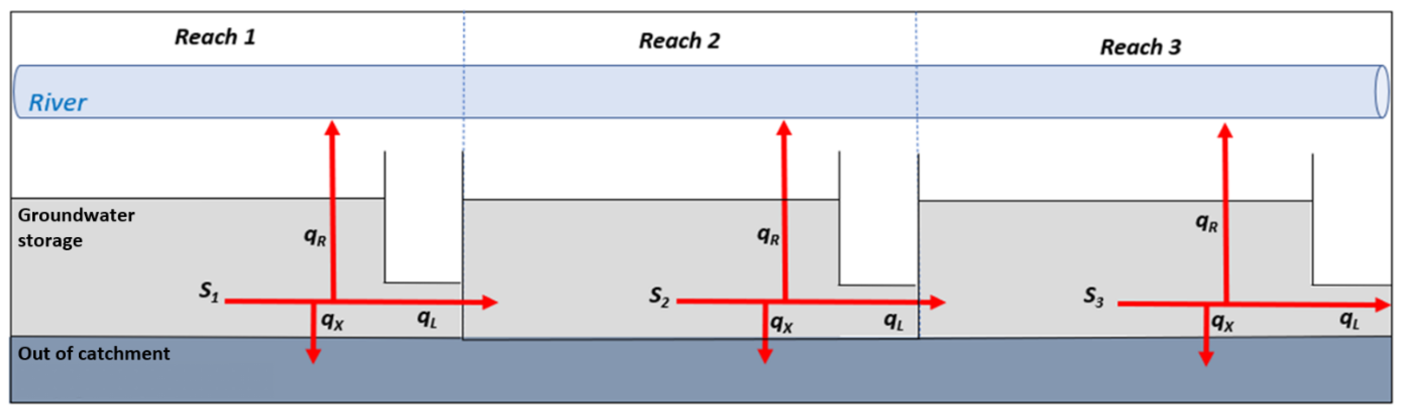
TopNet-GW calculates lateral and vertical groundwater flux from groundwater storage capacity, hydraulic conductivity, river flow, and river channel dimensions. Flow (q) from any sub-catchment consists of three components: lateral flow to up to two downstream or adjacent groundwater sub-catchments (q_l); vertical flow to (or from) the river channel (q_r); and vertical flow to deeper groundwater (q_x)):

$$\mathrm{q}={ \mathrm{q}}_{\mathrm{l}}+{\mathrm{q}}_{\mathrm{r}}+{\mathrm{q}}_{\mathrm{x}}$$

(1)

Figure 1 illustrates the direction of flows in three adjacent groundwater sub-catchment stores (S₁, S₂, and S₃), where q_l is the lateral flow between groundwater sub-catchments, q_r is the flow between shallow groundwater and the river, and q_x is the vertical loss from the groundwater sub-catchment store.

Each outflow component from a groundwater sub-catchment (q_l, q_x, and q_r, each with units of m/s) is assumed to be a linear function of groundwater stored in the sub-catchment (S, with units of m) such that:

$${\mathrm{q}}_{\mathrm{l}}=-{\mathrm{k}}_{\mathrm{l}} \mathrm{S}$$

(2)

where k_L is a lateral discharge coefficient [s⁻¹],

$${\mathrm{q}}_{\mathrm{r}}=-{\mathrm{k}}_{\mathrm{r}} \mathrm{S}$$

(3)

where ${\mathrm{k}}_{\mathrm{R}}$ is the river discharge coefficient [s⁻¹],

$${\mathrm{q}}_{\mathrm{x}}=-{\mathrm{k}}_{\mathrm{x}} \mathrm{S}$$

(4)

and where ${\mathrm{k}}_{\mathrm{X}}$ is the deep groundwater percolation coefficient [s⁻¹].

As a result, outflow from each groundwater sub-catchment $\left(\mathrm{q}\right)$ can be described by a one-dimensional flow vector and is a function of stored groundwater ($\mathrm{S}$) such that:

$$\mathrm{q}=-\mathrm{K} \mathrm{S}$$

(5)

where K_lrx is a groundwater discharge coefficient (s⁻¹) of the sub-catchment.

It follows that:

$$\mathrm{K}={ \mathrm{k}}_{\mathrm{l}}+{ \mathrm{k}}_{\mathrm{r}}+{\mathrm{k}}_{\mathrm{x}}$$

(6)

and thus

$${\mathrm{q}}_{\mathrm{l}}=\frac{{\mathrm{k}}_{\mathrm{l}}}{\mathrm{K}} \mathrm{q}$$

(7)

$${\mathrm{q}}_{\mathrm{r}}=\frac{{\mathrm{k}}_{\mathrm{r}}}{\mathrm{K}} \mathrm{q}$$

(8)

$${\mathrm{q}}_{\mathrm{X}}=\frac{{\mathrm{k}}_{\mathrm{X}}}{\mathrm{K}} \mathrm{q}$$

(9)

To simplify further, we can also describe each flow coefficient ratio as a single variable (f):

$${\mathrm{f}}_{\mathrm{l} }=\frac{{\mathrm{k}}_{\mathrm{l}}}{\mathrm{K}}$$

(10)

$${\mathrm{f}}_{\mathrm{r}}=\frac{{\mathrm{k}}_{\mathrm{r}}}{\mathrm{K}}$$

(11)

$${\mathrm{f}}_{\mathrm{x}}=\frac{{\mathrm{k}}_{\mathrm{x}}}{\mathrm{K}}$$

(12)

and

$${\mathrm{f}}_{\mathrm{l}}+{ \mathrm{f}}_{\mathrm{r}}+{ \mathrm{f}}_{\mathrm{x}}=1$$

(13)

We introduce the flow coefficient ratios because, with the limited information available, it is more practical to estimate a single outflow coefficient (K) and some ratios of flows (f) rather than several outflow coefficients.

2.1. Parameterization Scheme

National-scale datasets used to parameterize the above model include the New Zealand Groundwater Atlas [26] and water-table map [27,28,29]; QMAP 1:250,000 national geological map of New Zealand [13,30]; the New Zealand Aquifer Map [31]; and the NZ River Maps hydrology, ecology, and water quality metrics [32]. Derived parameters from these coverages include depth to groundwater, porosity, and hydraulic conductivity [11,26,27]; river-bed dimensions, sediment type, and river-bed hydraulic conductivity; and surface–groundwater interaction [11]. Figure 2 illustrates steps in the parameterization schema and datasets used.

The national water-table map [27,28,29] also describes static water-table head (from which flow direction can be derived), sub-catchment scale saturated hydraulic conductivity (K_sat), and groundwater storage (S). River-bed hydraulic conductivity and channel width [32] were used to determine the river discharge coefficient (k_r) and lateral flow coefficient (k_l) for each reach.

Estimation of parameter sets was performed for each regional administration boundary to allow a national-scale model to be run by the region and to promote model adoption by local government agencies.

2.1.1. Surface–Groundwater Interaction (q_r)

There are three potential methods to estimate flow between the surface and groundwater sub-catchments:

Flow rate can be described as the average fraction of river flow to groundwater, such that:

$${\mathrm{q}}_{\mathrm{r}}={- \mathrm{f}}_{\mathrm{r}} {\mathrm{q}}_{\mathrm{sf}}$$

(14)

where f_l ∈ [0, 1], q_sf is the surface water flow, and f_r can be determined from long-term river flow accretion data (i.e., variation in q_r relative to q_sf).

• NZ River Maps [32] coverage can be used to say that:

$${\mathrm{q}}_{\mathrm{r}}=-\mathrm{W} \mathrm{L} {\mathrm{K}}_{\mathrm{b}\mathrm{e}\mathrm{d}}$$

(15)

where W and L are river-bed width and length, and K_bed is the hydraulic conductivity of the river-bed [12].

2.

Like the above method but uses river depth such that:

$${\mathrm{q}}_{\mathrm{r}}=- \mathrm{g}\left(\mathrm{river}\right) \mathrm{W} \mathrm{L} {\mathrm{K}}_{\mathrm{bed}}$$

(16)

where g(river) is the fraction of river depth lost to groundwater per timestep.

2.1.2. Lateral Groundwater Flow (q_l)

The lateral groundwater flow coefficient (f_l) is simplified such that:

• f_l = 1 when water flows from the river to groundwater (‘losing reach’);
• f_l = 0 when water flows from groundwater to the river (‘gaining reach’).

However, f_l can be given a value between 0 and 1 if prior information is available; thus, f_l ∈ [0, 1].

2.1.3. Flow to Deeper Groundwater (q_x)

Groundwater loss (to a non-returnable deeper groundwater zone) can be estimated using a simple water balance equation. Knowledge of other hydrological fluxes (rainfall, runoff, and evapotranspiration) can be used to calculate this term if losses are expected and there is insufficient reliable hydrogeological information available. Under most circumstances, a ‘closed catchment’ is assumed (i.e., f_x = 0) unless evidence suggests otherwise.

2.1.4. Flow Coefficients

The sum of the flow coefficients (Equation (6)) can be estimated from hydraulic conductivity and porosity data derived from the New Zealand groundwater Atlas [26,27]. Aquifer near-surface hydraulic conductivity (K) is defined [29,33] and calculated using:

$$\mathrm{K}={\mathrm{K}}_0{\mathrm{e}}^{-\mathrm{z}/\mathrm{c}}$$

(17)

where K₀ is the hydraulic conductivity at or near the surface, z is the depth, and c is a function of terrain slope, climate, geology derived from mechanical and chemical denudation, and tectonic uplift rates of large sedimentary basins defined by the following equation:

$$\mathrm{c}=\frac{\mathrm{a}}{1+(\mathrm{b}\times \mathrm{s})}; \mathrm{c} \ge {\mathrm{c}}_{\min }$$

(18)

where s is the terrain slope and a, b, and c_min are constants set to 75, 150, and 4, respectively [30]. The resulting K_sat values range from 0 to 87 m/day. Porosity (φ_z) at depth (z) is derived using the relationship described for sandstone and shales with clay dependence [34] such that:

$${\mathsf{\Phi }}_{\mathrm{z}} ={\mathsf{\phi }}_0 \exp (-0.001\mathrm{z}(0.23+0.27\mathrm{Cl}))$$

(19)

where z is depth, and φ₀ is effective porosity at the surface. Cl is the percentage clay factor, resulting in porosity ranging from 0 to 32%.

Both K_sat and storage (S) (calculated from porosity and estimated aquifer volume) are assumed to decrease with depth (z) below the surface. If we assume that the aquifer behaves like a linear reservoir, the characteristic hydraulic response time will be 1/$\mathrm{K}$, so that:

$$\mathrm{K} =\frac{{\mathrm{K}}_{\mathrm{sat}}\left(\mathrm{z}\right)}{\mathrm{L}\times \mathrm{S}\left(\mathrm{z}\right)}$$

(20)

If the equilibrium water table is at depth z, then hydraulic conductivity and porosity are evaluated with respect to that depth. As both K_sat(z) and S(z) are available at 200 m grid resolution of the water-table map, K can be calculated for individual TopNet-GW sub-catchment modeling units (i.e., Strahler order 1 or 3 catchments of approximately 0.5 km² and approximately 10 km², respectively).

If K is known, then only two out of the three flow ratio parameters f_l, f_r, and f_x described in Equations (10)–(12) need to be estimated, as the third parameter can be calculated from Equation (13). As it is generally easier to obtain estimates of flow between the river and groundwater store (for example, through streamflow accretion survey or borehole monitoring) compared to an estimation of flow to the deeper groundwater store, f_l and f_r are estimated rather than f_x.

For losing reaches (that exhibit a nett transfer of water from the river to groundwater), flow from shallow groundwater to the river (k_r) is zero, but there may be a lateral flow between each shallow groundwater catchment so that:

$${\mathrm{k}}_{\mathrm{r}}=0$$

(21)

$${\mathrm{k}}_{\mathrm{l}}=\mathrm{K}$$

(22)

For gaining reaches (that exhibit a nett transfer of water from groundwater to river), there will be a higher flow per unit area than is suggested by the larger aquifer water balance as not all the area of the aquifer is producing flow into the river. If a_l and a_g are the areas of the catchment with losing and gaining reaches, respectively, then we can say that:

$${\mathrm{k}}_{\mathrm{r}}=\mathrm{K} \frac{{\mathrm{q}}_{\mathrm{r}}}{\mathrm{q}}\times \frac{{\mathrm{a}}_{\mathrm{l}}+{\mathrm{a}}_{\mathrm{g}}}{{\mathrm{a}}_{\mathrm{g}}}$$

(23)

$${\mathrm{k}}_{\mathrm{l}}=\mathrm{K}\frac{{\mathrm{q}}_{\mathrm{l}}}{\mathrm{q}}$$

(24)

2.2. Regional Geology

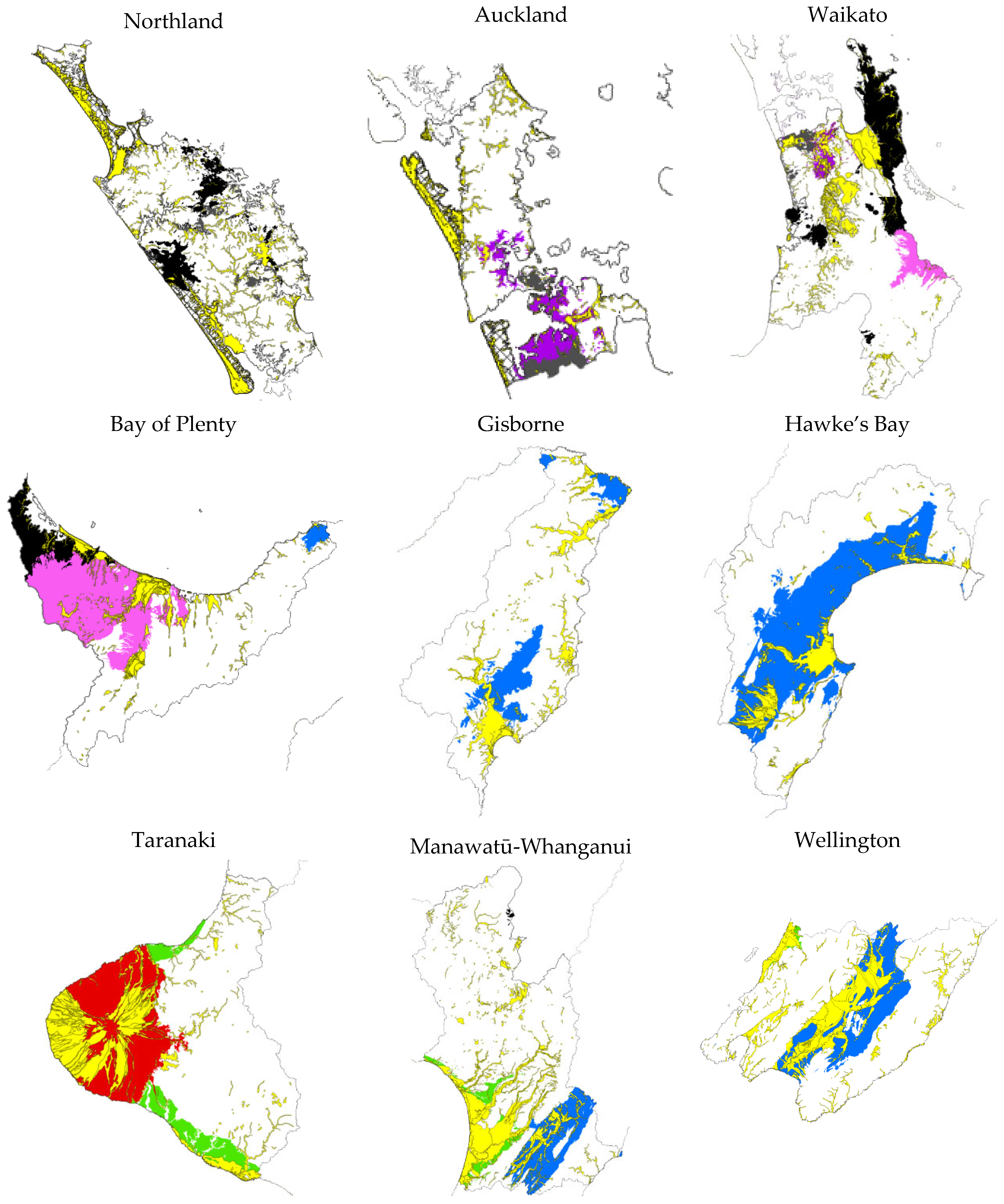
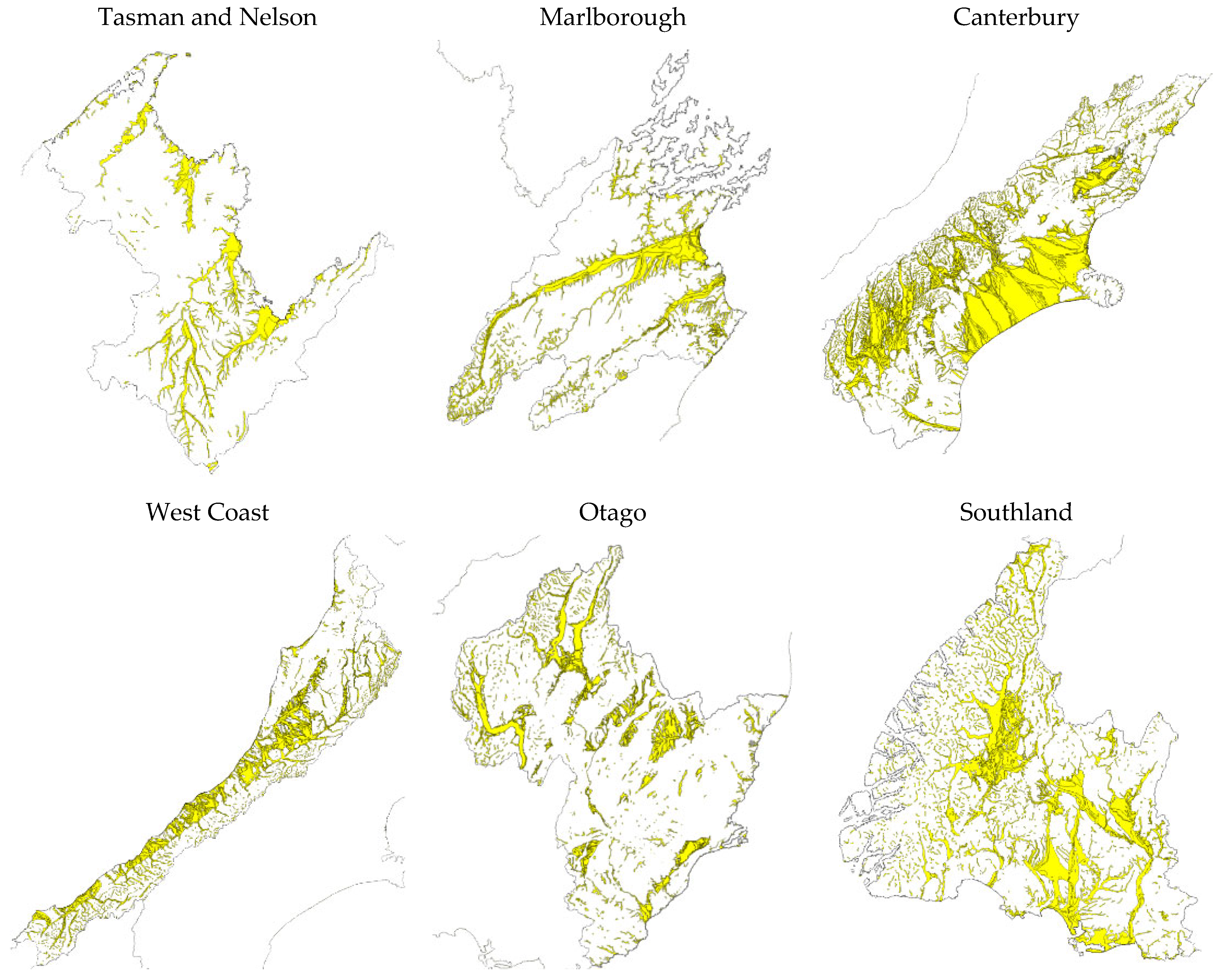
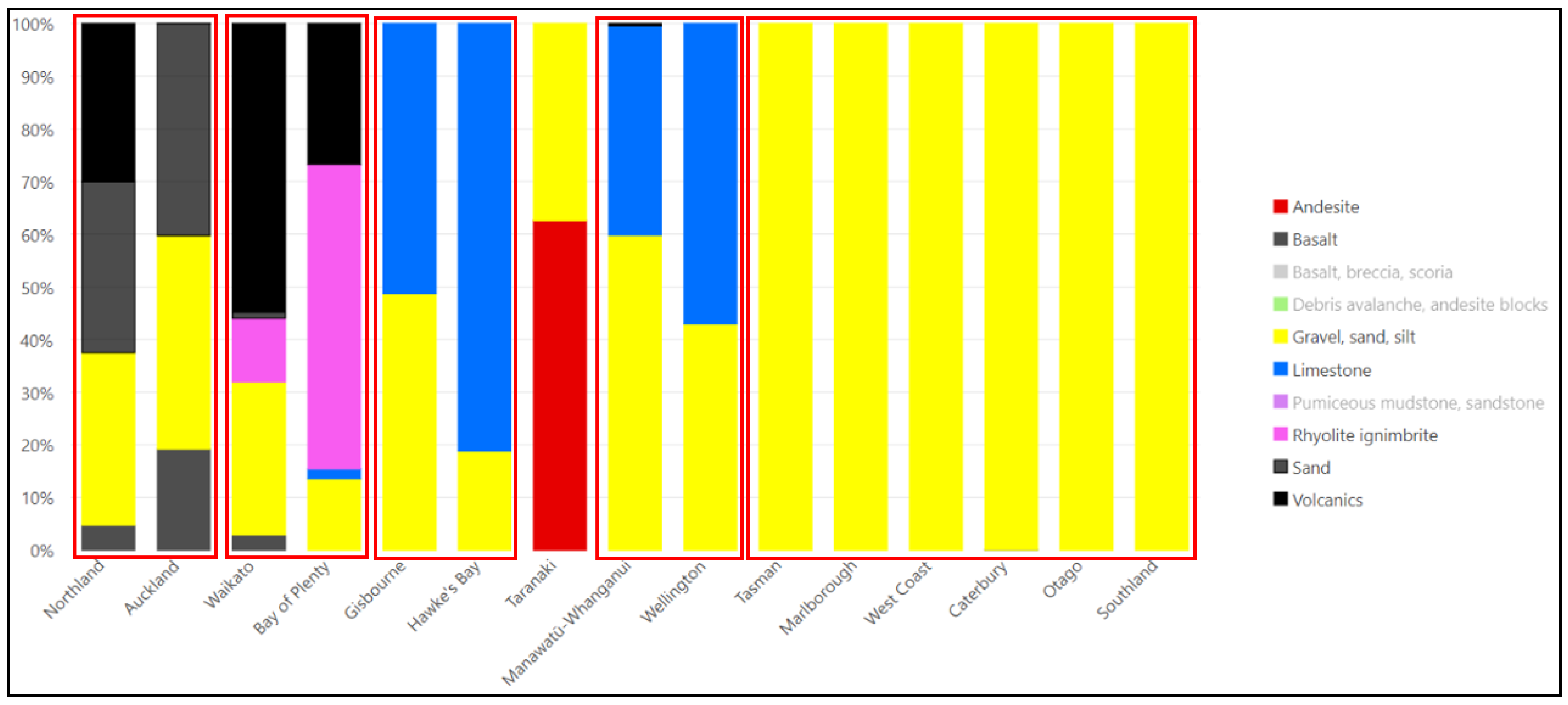
Figure 3 and Figure 4 illustrate the distribution of lithology type within aquifers in each administrative region of New Zealand. Similarities in aquifer lithology between regions [35] suggest that model parameterization can be simplified by using combined region parameter sets. Northland is characterized by sand, silt and gravel, and volcanic aquifers. Surface–groundwater interaction increases around the perimeter of the basalt and greywacke formations. Groundwater recharge typically occurs in upland areas, which then drain via springs in the foothills and to the lower valleys. Aquifers in the region are characterized as either quaternary coastal aquifers or inland volcanic aquifers. Auckland, to the south, differs slightly in that most groundwater abstraction is from the geothermal and volcanic basalt aquifers. MODFLOW and MIKE-SHE have been used [36] to model the hydrogeological response of the unconfined fractured basalt and semi-confined sandstone and mudstone aquifer systems.

The Waikato region can be divided geologically into three formations (alluvial deposits, volcanic, and sedimentary). The location and extent of groundwater availability are reflected in the location of consented groundwater takes, which are predominantly found in alluvial deposits [37]. The Bay of Plenty region, which is dominated by rhyolite and ignimbrite lithology, with gravel, sand, and silts aquifers towards the coast, can be divided into three major groundwater catchments (Rangitikei, Tarawera, and Whakatāne). Significant parts of this region have previously been modeled by [38,39,40,41]. Other models include a MODFLOW transient model for the Kaituna water management area [42], a flow and transport model for Tarawera [43], and a Western Bay of Plenty groundwater flow model [44].

The aquifers within the Gisborne region surround Poverty Bay Flats, where over 1400 bores draw water for irrigation and domestic use from the gravel, silt, and sand aquifers [45,46]. Except for the Te Hapara aquifer, none of the known sand aquifers have a direct connection to the sea [46]. It is worth noting that 51% of aquifers in the region are ‘limestone’, which feeds into gravel flats or flows directly to the coast. All rivers close to the coast are likely to recharge groundwater in alluvial valleys and sand dune systems.

Hawke’s Bay region exhibits similar aquifer systems (Heretaunga Plains and Ruataniwha Basin). The former is an alluvial plain formed by sediments deposited by the Ngaruroro, Tukituki, and Tūtaekurī Rivers [47]. The Waipawa River through the Ruataniwha Plains indicates losses to groundwater of around 2.2 m³/s [48,49,50,51,52]. With 81% of the defined aquifers in the region classed as ‘limestone’, rivers generally lose water to the aquifer upstream and gain water downstream.

Taranaki is different from all other North Island regions as it is dominated by andesitic volcanic cones. It has five principal aquifer systems named after the geological formations (Matemateāonga, Whenuakura, Tāngāhoe, Marine Terraces, and Taranaki Volcanics). Shallow groundwater is extracted from volcanic deposits and marine terraces east of New Plymouth and along the SW coast towards Wanganui [53], whereas deeper groundwater (>200 m bgl) is extracted from Tertiary sediments in north Taranaki.

The Upper Hutt aquifer in the Wellington region receives recharge from the Hutt River between Maoribank Bend and 700 m upstream of the Whakatikei confluence [30]. Data suggest that 500–600 L/s is lost between Maoribank Bend and Pine Ave [46]. The river crosses the Wellington Fault at Moonshine Bridge, where the riparian geology changes from low-permeability Pleistocene fan and alluvium deposits to more-permeable Holocene alluvium. The river provides significant recharge to the unconfined alluvial gravel aquifer upstream of the Whakatikei River confluence [54,55,56,57,58]. Other significant aquifer bodies in the region include the Wairarapa [59,60,61] and Kapiti Coast [62].

Like the Wellington region, the general direction of groundwater movement in the Horizons (Manawatū-Whanganui) region is from the inland hills towards the coast. The strata of the region consist of three main sequences: i. the geological basement made up of low permeability and heavily inundated greywacke (Ruahine and Tararua Ranges); ii. fine-grained marine sedimentary strata comprised of low permeability siltstone and/or mudstone; and iii. alluvial deposits formed by the erosion of the greywacke ranges. Thirty-eight percent of the region’s aquifers are classed as limestone, with the remainder being gravel, sand, and silts.

In the South Island, virtually all aquifers are classed as ‘gravel, silt or sand’. Whilst this should make parameterization easier, the ‘gravel, silt or sand’ classification is large, so refinement of derived model parameters may be required at the sub-catchment scale.

3. Results

Figure 5 illustrates the similarity between neighboring regions of Northland and Auckland; Waikato and Bay of Plenty; Gisborne and Hawkes Bay; and Wellington and Manawatū-Whanganui. The extent of these similarities and the case for combined region parameter sets is described below.

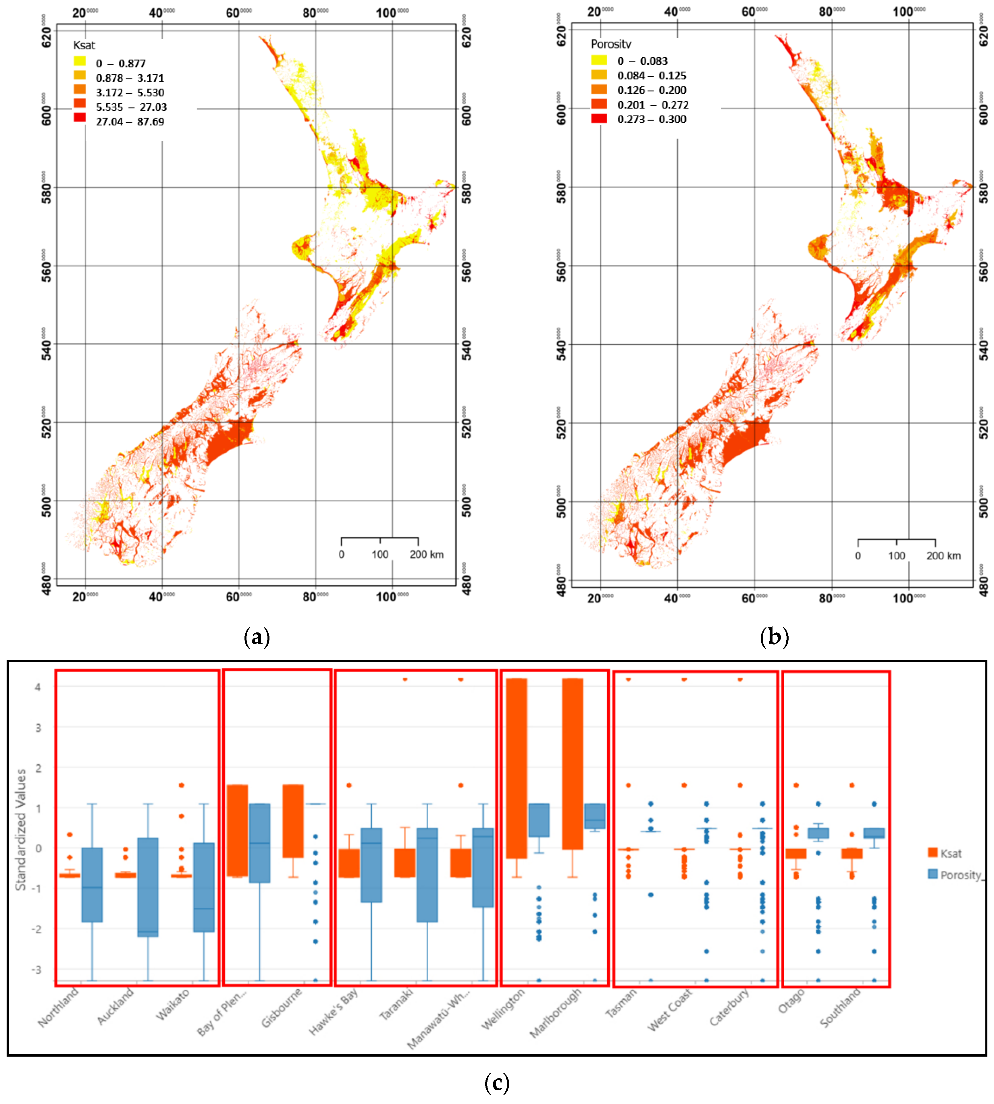
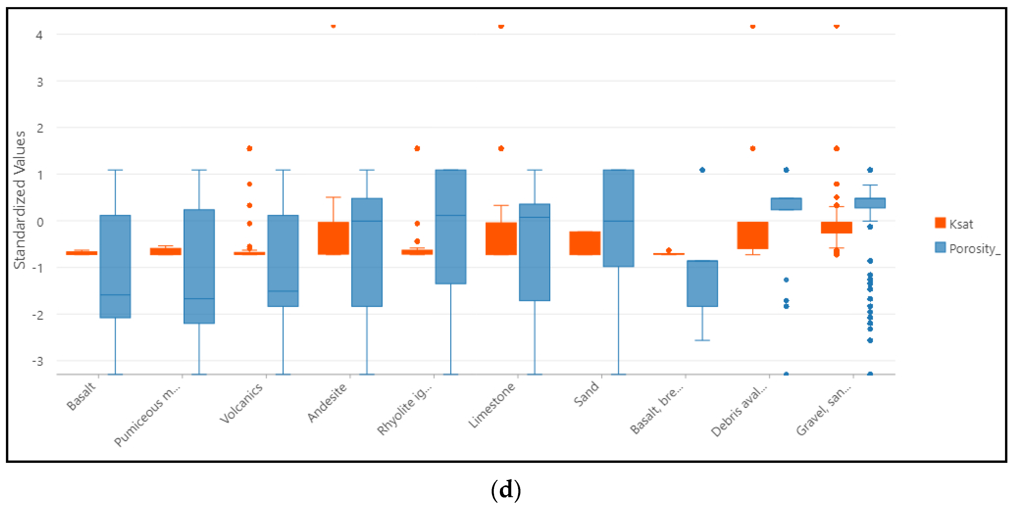
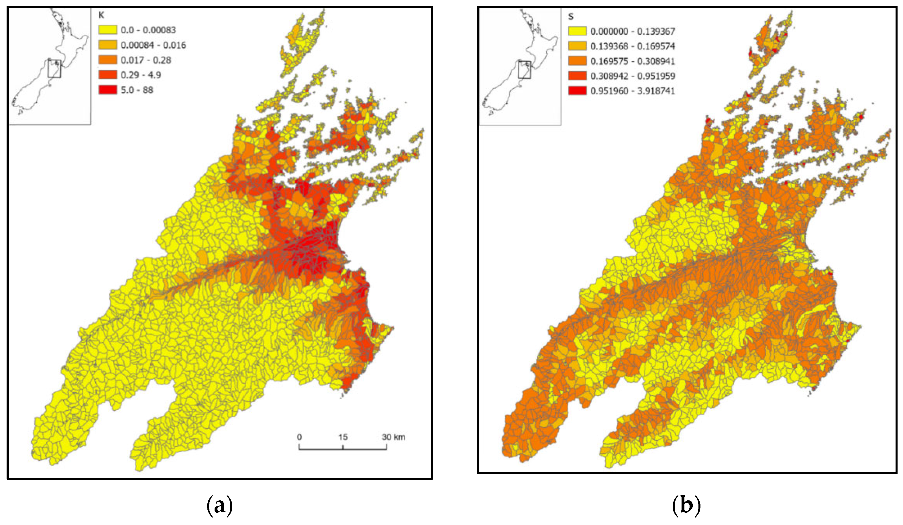
Additional quantitative analysis of known parameter ranges (e.g., K_sat and porosity) can aid in the estimation of derived parameter sets. Figure 6a,b, for example, illustrate the distribution of near-surface hydraulic conductivity and porosity.

Standardized values of each parameter are plotted to illustrate the variability of each parameter relative to rock type and region. Correlation between the hydraulic conductivity and porosity were calculated for each rock type and region, with strongest correlations occurring in basalt (R² = 0.97), basalt/breccia/scoria (R² = 0.93), and pumice/mudstone/sandstone (R² = 0.87) rock types, and in Taranaki (R² = 0.87), Gisborne (R² = 0.63); Southland (R² = 0.59), and Bay of Plenty (R² = 0.59) regions. Notably, there is limited correlation in the South Island regions, which, despite having a single geology type (gravel, sand, silt), have very large variability in values of both hydraulic conductivity and porosity. This leads to greater uncertainty in parameterization in those regions.

From the above analysis and description, it can be seen that adjacent regions may show some similarity in derived model parameter values (K_sat and porosity) (Figure 6c). This happens because the dominant geology of any region, which is a primary control of ground surface parameters, often runs across the administrative region boundaries. This can also be seen at a national scale, as the variability of surface parameters is defined by underlying aquifer geology (Figure 6d). Regions with the most similar geology, and hence parameters, include Northland–Auckland–Waikato; Bay of Plenty–Gisborne; Hawke’s Bay–Taranaki–Manawatū–Whanganui; Wellington–Marlborough; Tasman–West Coast–Canterbury; and Otago–Southland.

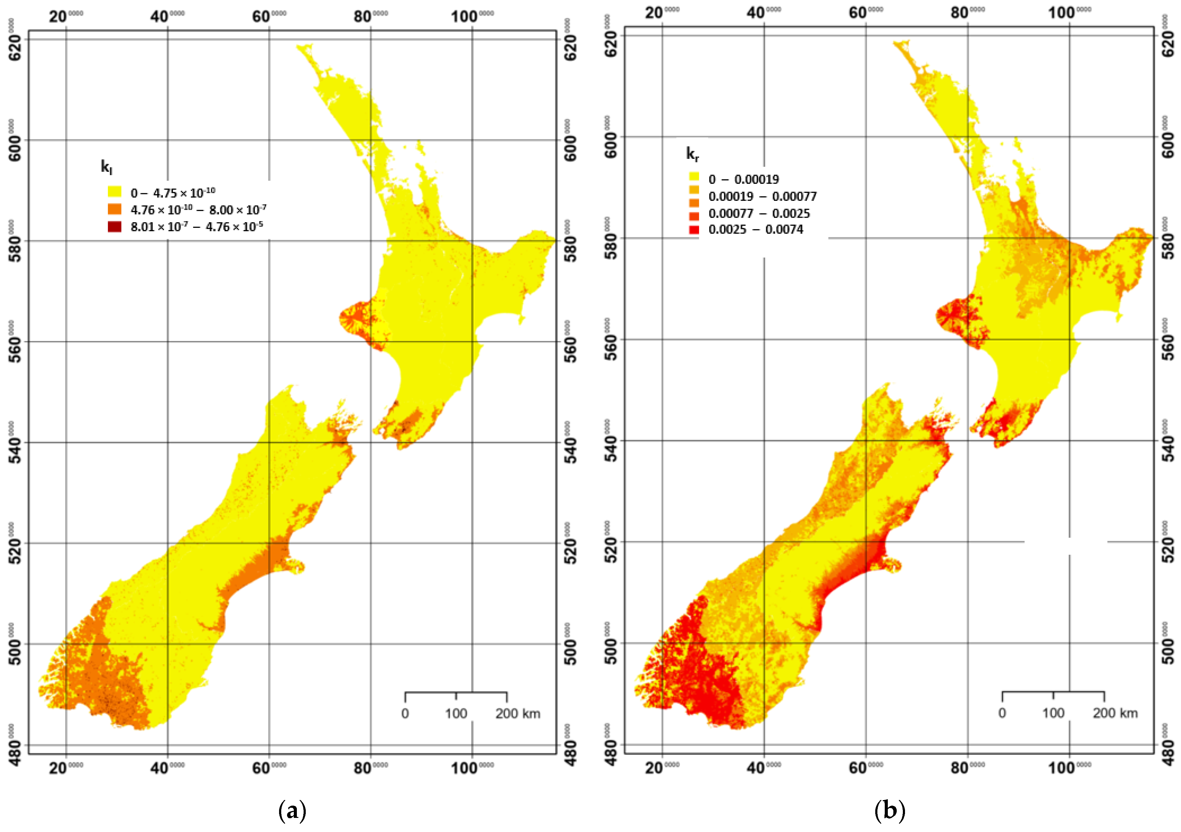
The resulting vertical (k_r) and lateral (k_l) hydraulic conductivity coefficients for losing and gaining reaches (as defined in Equations (21)–(24)) are illustrated in Figure 7. The distribution of the lateral flow coefficient (k_l) more strongly reflects the variation in geological and land surface parameters, whereas the vertical coefficient is controlled by the extent of surface–groundwater interaction.

3.1. Uncertainty

Whilst regional councils in New Zealand have both surface and groundwater monitoring networks, there remains much uncertainty in the total extent and magnitude of surface–groundwater interaction [63]. Surface–groundwater interaction in New Zealand predominantly occurs after rivers have emerged from the high mountain ranges and as they flow across alluvial plains. River flow depletion and accretion surveys can be used to estimate the magnitude of surface–groundwater flow, but this tends to be spatially and temporally dynamic, as it is dependent on local geological variability and sub-surface hydraulic connectivity [64].

The parameter sets outlined in this study inherit assumptions contained within the hydrogeological datasets from which they are derived. For example, the surface–groundwater interaction map [9] is based on the assumption of three characteristic landscape types, including permeable headwaters (accreting rivers), inland flood plains (depleting rivers), and accreting rivers (coastal catchments). As a result, only sub-catchments within these landscape types are defined as active groundwater catchments within the parameter datasets.

Simulated river flow from the TopNet-GW model has been shown to be most sensitive to hydraulic conductivity between the river and aquifer (k_r) [9]. However, simulations are also sensitive to the extent of shallow aquifer zone and lateral groundwater flow (k_l). Thus, whilst we would expect river flow to be most sensitive to k_r, it will be mitigated by k_l to an extent dependent on the existence of a shallow aquifer layer and the aquifer storage potential (represented by porosity).

The uncertainty associated with the parameter estimation method used is related to the water-table depth map [30], which assumes a state of equilibrium within modeled aquifers. The implication of this is that the derived flow coefficients k_r and k_l underestimate flow gradients during model simulations of rapid groundwater depletion or recharge. The impact of this uncertainty can be reduced through local-scale calibration and validation through field study. Similarly, the derivation of depth to hydraulic basement value was based on the analysis of large-scale fluvial sedimentary basins [30]. Thus, the estimates of sub-surface hydraulic conductivity made for other landform types (e.g., small coastal basins or volcanic aquifers) are susceptible to greater uncertainty (as estimates were based on hydraulic depth to basin). The authors also noted that no consideration of the impact of the potential of confining layers or material anisotropy on hydraulic conductivity was made.

3.2. Case Study: Marlborough, NZ

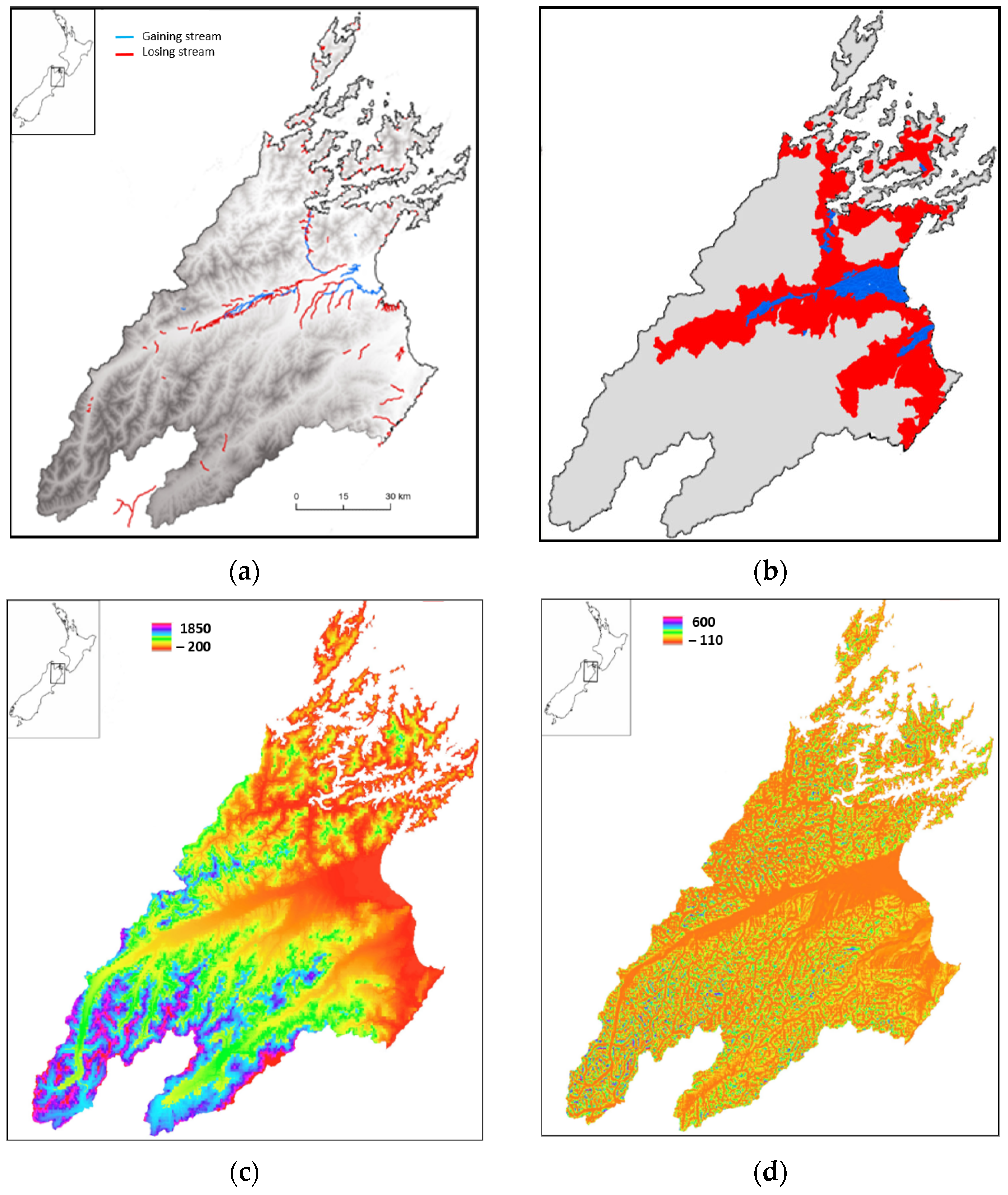
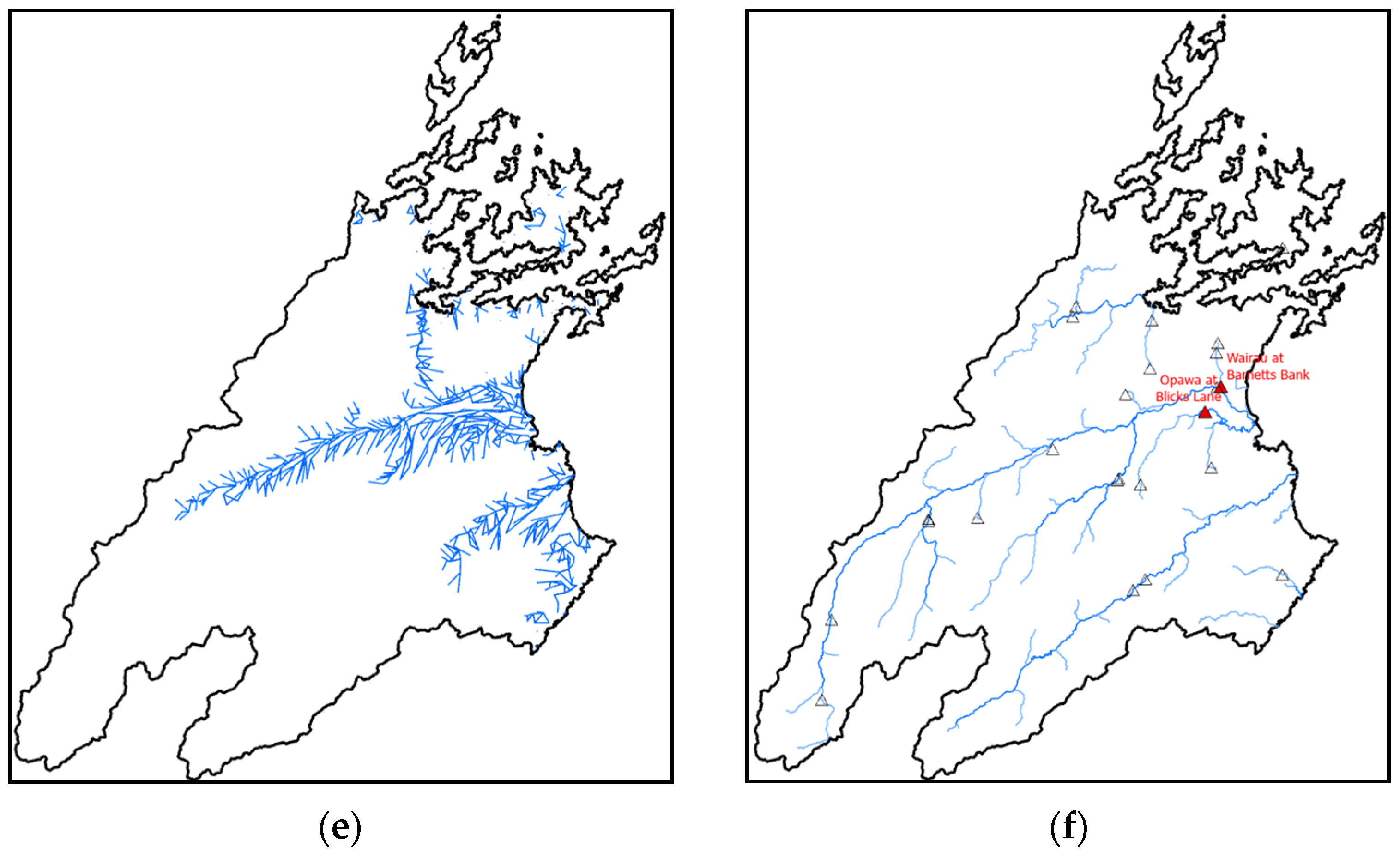
The above datasets were used to parameterize TopNet-GW for the Marlborough region (South Island). The locations of river catchments that exhibit surface–groundwater interaction [9] are shown in Figure 8a,b. The mean annual groundwater head (m above mean sea level) and depth to water table (m below ground level) (as defined by the water-table map [27]) are shown in Figure 8c,d. Dominant groundwater flow direction is derived from the distribution of mean annual groundwater head (Figure 8e), and the location of gauged streams in Marlborough is shown in Figure 8f.

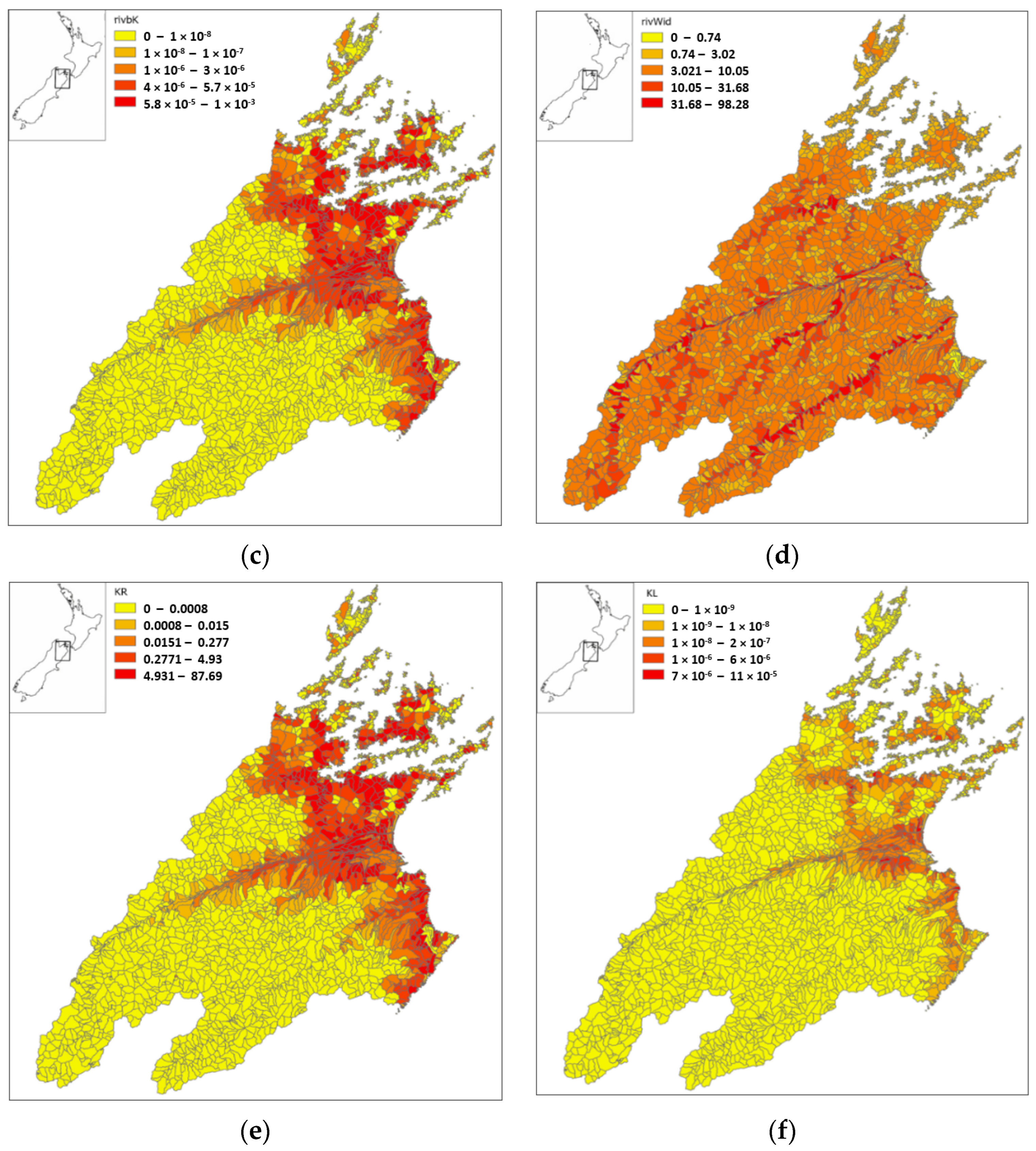
Figure 9a,b illustrate distributions of conductivity (K) and aquifer storage (S) for the region, as derived from the water-table height, river-bed conductivity, and channel width (Figure 9c,d).

Figure 9e,f show coefficients of vertical and lateral flow (k_r and k_l). It can be seen that k_r and river-bed conductivity are spatially correlated as river-bed permeability is a direct control of surface–groundwater interaction through the river channel.

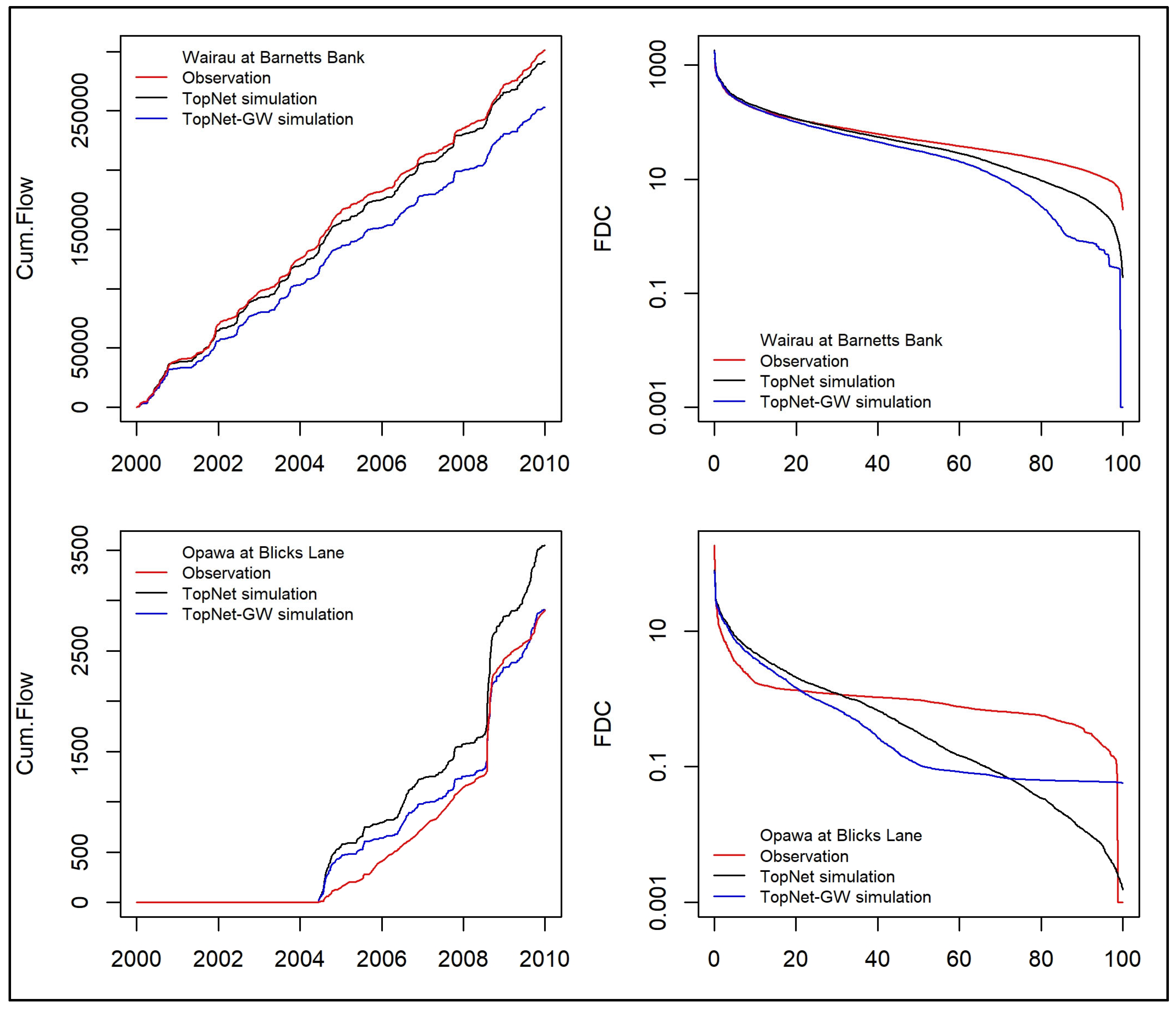
To assess the utility of the above parameter sets for groundwater modeling, TopNet-GW was run for the Marlborough region for the period 2000 to 2010. The performance of the TopNet_GW model was then compared to the TopNet surface water model and observed data in the Wairau River and Opawa River (see Figure 10). Both models performed well in the larger Wairau River catchment (Nash–Suttcliff Efficiency (NSE)—0.64). Performance was worse in the smaller Opawa River (NSE = 0.3).

The flow duration curves and cumulative flow diagrams in Figure 10 illustrate how each model replicates annually averaged flow characteristics. Both TopNet-GW and TopNet models underestimate lower quartile flows in the Wairau River. This indicates that the models are over-predicting ‘leakage’ from the river to the groundwater store. By contrast, in the Opawa River catchment (modeled from mid-2004), both models overestimate peak flows. The TopNet-GW model performs better than the TopNet model, which underestimates low flows to a greater extent.

4. Discussion

The parameterization scheme described above is used to produce a reach-scale groundwater-model parameter set for aquifers in New Zealand. Vertical and lateral hydraulic conductivity and aquifer storage are defined from hydrogeological data. Whilst the method is globally reproducible, there are several features in the approach that are dependent on the availability of key datasets.

For example, the method uses a high-resolution digital elevation model (DEM) to define a hydrologically continuous drainage network. National coverages of geological data, aquifer locations, and surface water catchment boundaries, which are available in most countries, are then defined relative to the DEM. By contrast, river channel characteristics, river-bed conductivity, and estimates of depth to groundwater may be more difficult to identify at the required resolution.

Comparison of model parameters and output relative to different aquifers in New Zealand is likely to yield varying results, as local or regional scale aquifer models may be of varying resolution, extent, and spatial variability. Whilst outside the scope of this study, it is envisaged that such a comparison will help inform the refinement of model parameter sets in the future.

In the case study for the Marlborough region, the performance of the parameter set, as represented by the TopNet-GW model output, is regionally specific, and results cannot be assumed to be representative of the whole country. Future research will assess the spatial variability of model output along river profiles within aquifer areas and the seasonal variability in surface–groundwater interaction, as determined by water-table fluctuation, and compare model internal variables with observed groundwater height variation.

A significant drawback of the existing parameter set is that it has been developed with reference to a steady-state surface–groundwater interaction map. As a result, modeled groundwater flow is unidirectional, either as flow from the river to the groundwater store or as flow from the groundwater store to the river. This reduction in model complexity results in lower hydrograph peaks and elevated low-flow characteristics.

The results of this research build on the conceptual understanding of previous work that identified potential groundwater recharge zones. Whilst there is some overlap in methodology with the previous study (same land-use, soil, geology, and topographic data), both studies identify the potential and relative magnitude of groundwater recharge. In this study, the component datasets were further aggregated to provide a reach-scale characterization of subsurface properties.

5. Conclusions

An a priori parameterization method was developed for the TopNet-GW model that allowed it to be applied in ungauged catchments in New Zealand. A nationwide parameter set was produced to represent regional aquifer storage behavior and groundwater flux. When the model was applied in the Marlborough region, it performed well in predicting low flows but less well in predicting peak flows. The performance of the model indicated that the spatial distribution of groundwater processes is correct but that local scale calibration may be required to improve model accuracy.

Improved a priori parameter identification may be achieved by using additional hydrogeological data (such as the aquitard and aquiclude layers and their associated properties). However, in the first instance, a more thorough assessment of the spatial variation in model performance and parameter uncertainty across all regions of New Zealand is required.

References

- Demissie, Y.; Valocchi, A.; Cai, X.; Brozovic, N.; Senay, G.; Gebremichael, M. Parameter estimation for groundwater models under uncertain irrigation data. Groundwater 2015, 53, 614–625. [Google Scholar] [CrossRef] [PubMed]
- Flinck, A.; Folton, N.; Arnaud, P. Assimilation of piezometric data to calibrate parsimonious daily hydrological models. Water 2021, 13, 2342. [Google Scholar] [CrossRef]
- Klaas, D.K.; Imteaz, M.; Sudiayem, I.; Klaas, E.M.; Klaas, E.C. Parameterisation of physical models to configure subsurface characteristics of groundwater basins. Groundw. Sustain. Dev. 2019, 9, 100255. [Google Scholar] [CrossRef]
- Yang, J.; McMillan, H.; Zammit, C. Modeling surface water–groundwater interaction in New Zealand: Model development and application. Hydrol. Process. 2017, 31, 925–934. [Google Scholar] [CrossRef]
- Bandaragoda, C.; Tarboton, D.; Woods, R. Application of TopNet in the distributed model intercomparison project. J. Hydrol. 2004, 298, 178–201. [Google Scholar] [CrossRef]
- Clark, M.P.; Nijssen, B.; Lundquist, J.D.; Kavetski, D.; Rupp, D.E.; Woods, R.A.; Freer, J.E.; Gutmann, E.D.; Wood, A.W.; Brekke, L.D.; et al. A unified approach for process-based hydrologic modeling: 1. Modeling concept. Water Resour. Res. 2015, 51, 2498–2514. [Google Scholar] [CrossRef]
- McMillan, H.; Freer, J.; Pappenberger, F.; Krueger, T.; Clark, M. Impacts of uncertain river flow data on rainfall-runoff model calibration and discharge predictions. Hydrol. Process. 2010, 24, 1270–1284. [Google Scholar] [CrossRef]
- Booker, D.J.; Woods, R.A. Comparing and combining physically-based and empirically-based approaches for estimating the hydrology of ungauged catchments. J. Hydrol. 2014, 508, 227–239. [Google Scholar] [CrossRef]
- Yang, J.; Griffiths, J.; Zammit, C. National classification of surface–groundwater interaction using random forest machine learning technique. River Res. Appl. 2019, 35, 932–943. [Google Scholar] [CrossRef]
- Srinivasan, M.S.; Tschritter, C.; Morgan, L.; Weaver, L. Applied hydrology: Key science and research developments in the last ten years. J. Hydrol. 2021, 60, 19–37. [Google Scholar]
- Johnson, P.; Tschritter, C.; Mourot, F.; Weir, J.; Rawlinson, Z.J. New Zealand Groundwater Atlas: 3D Groundwater Models around New Zealand (A Review); Ministry for the Environment: Wellington, New Zealand, 2019. [Google Scholar]
- Bidwell, V.J. Realistic forecasting of groundwater level, based on the eigen structure of aquifer dynamics. Math. Comput. Simul. 2005, 69, 12–20. [Google Scholar] [CrossRef]
- White, J.T. A model-independent iterative ensemble smoother for efficient history-matching and uncertainty quantification in very high dimensions. Environ. Model. Softw. 2018, 109, 191–201. [Google Scholar] [CrossRef]
- Toews, M.W.; Daughney, C.J.; Cornaton, F.J.; Morgenstern, U.; Evison, R.D.; Jackson, B.M.; Petrus, K.; Mzila, D. Numerical simulation of transient groundwater age distributions assisting land and water management in the Middle Wairarapa Valley, New Zealand. Water Resour. Res. 2016, 52, 9430–9451. [Google Scholar] [CrossRef]
- Wöhling, T.; Gosses, M.J.; Wilson, S.R.; Davidson, P. Quantifying River-Groundwater Interactions of New Zealand’s Gravel-Bed Rivers: The Wairau Plain. Groundwater 2018, 56, 647–666. [Google Scholar] [CrossRef]
- Rajanayaka, C.; Woodward, S.J.R.; Lilburne, L.; Carrick, S.; Griffiths, J.; Srinivasan, M.S.; Zammit, C.; Fernández-Gálvez, J. Upscaling point-scale soil hydraulic properties for application in a catchment model using Bayesian calibration: An application in two agricultural regions of New Zealand. Front. Water 2022, 4, 986496. [Google Scholar] [CrossRef]
- Snelder, T.H.; Biggs, B.J. Multiscale river environment classification for water resources management. JAWRA J. Am. Water Resour. Assoc. 2002, 38, 1225–1239. [Google Scholar] [CrossRef]
- Rattenbury, M.S.; Isaac, M.J. The QMAP 1:250,000 Geological Map of New Zealand project. N. Z. J. Geol. Geophys. 2012, 55, 393–405. [Google Scholar] [CrossRef]
- Lilburne, L.; Hewitt, A.; Webb, T.H.; Carrick, S. S-map: A new soil database for New Zealand. In Proceedings of the Super Soil 2004: Proceedings of the 3rd Australian New Zealand Soils Conference, Sydney, Australia, 5–9 December 2004; pp. 5–9. [Google Scholar]
- Markstrom, S.L.; Niswonger, R.G.; Regan, R.S.; Prudic, D.E.; Barlow, P.M. GSFLOW-Coupled Groundwater and Surface-water FLOW model based on the integration of the Precipitation-Runoff Modelling System (PRMS) and the Modular Ground-Water Flow Model (MODFLOW-2005). US Geol. Surv. Tech. Methods 2008, 6, 240. [Google Scholar]
- Bailey, R.T.; Wible, T.C.; Arabi, M.; Records, R.M.; Ditty, J. Assessing regional-scale spatio-temporal patterns of groundwater-surface water interactions using a coupled SWAT-MODFLOW model. Hydrol. Process. 2016, 30, 4420–4433. [Google Scholar] [CrossRef]
- Sridhar, V.; Billah, M.M.; Hildreth, J.W. Coupled surface and groundwater hydrological modeling in a changing climate. Groundwater 2018, 56, 618–635. [Google Scholar] [CrossRef]
- Bizhanimanzar, M.; Leconte, R.; Nuth, M. Modelling of shallow water table dynamics using conceptual and physically based integrated surface-water–groundwater hydrologic models. Hydrol. Earth Syst. Sci. 2019, 23, 2245–2260. [Google Scholar] [CrossRef]
- Yu, X.; Moraetis, D.; Nikolaidis, N.P.; Li, B.; Duffy, C.; Liu, B. A coupled surface-subsurface hydrologic model to assess groundwater flood risk spatially and temporally. Environ. Model. Softw. 2019, 114, 129–139. [Google Scholar] [CrossRef]
- Harbaugh, A.W. MODFLOW-2005, The US Geological Survey Modular Ground-Water Model: The Ground-Water Flow Process; US Department of the Interior, US Geological Survey: Reston, VA, USA, 2005; Volume 6.
- Westerhoff, R.S.; Tschritter, C.; Rawlinson, Z.J. New Zealand Groundwater Atlas: Depth to Hydrogeological Basement; GNS Science: Lower Hutt, New Zealand, 2014; 19p. [Google Scholar]
- Westerhoff, R.; White, P.; Miguez-Macho, G. Application of an improved global-scale groundwater model for water table estimation across New Zealand. Hydrol. Earth Syst. Sci. 2018, 22, 6449–6472. [Google Scholar] [CrossRef]
- Fan, Y.; Miguez-Macho, G.; Weaver, C.P.; Walko, R.; Robock, A. Incorporating water table dynamics in climate modeling: 1. Water table observations and equilibrium water table simulations. J. Geophys. Res. Atmos. 2007, 112, D10125. [Google Scholar] [CrossRef]
- Miguez-Macho, G.; Fan, Y.; Weaver, C.P.; Walko, R.; Robock, A. Incorporating water table dynamics in climate modeling: 2. Formulation, validation, and soil moisture simulation. J. Geophys. Res. Atmos. 2007, 112, D13108. [Google Scholar] [CrossRef]
- Heron, D.W. Geological Map of New Zealand 1:250,000: Digital Vector Data 2014, 2nd ed.; GNS Science: Lower Hutt, New Zealand, 2014. [Google Scholar]
- Tschritter, C.; Westerhoff, R.S.; Rawlinson, Z.J.; White, P.A. Aquifer Classification and Mapping at the National Scale—Phase 1: Identification of Hydrogeological Units; GNS Science: Lower Hutt, New Zealand, 2017; 52p. [Google Scholar]
- Whitehead, A.L.; Booker, D.J. Communicating biophysical conditions across New Zealand’s rivers using an interactive webtool. N. Z. J. Mar. Freshw. Res. 2019, 53, 278–287. [Google Scholar] [CrossRef]
- Gleeson, T.; Smith, L.; Moosdorf, N.; Hartmann, J.; Dürr, H.H.; Manning, A.H.; van Beek, L.P.H.; Jellinek, A.M. Mapping permeability over the surface of the Earth. Geophys. Res. Lett. 2011, 38, L02401. [Google Scholar] [CrossRef]
- Ramm, M.; Bjørlykke, K. Porosity/depth trends in reservoir sandstones: Assessing the quantitative effects of varying pore-pressure, temperature history and mineralogy, Norwegian Shelf data. Clay Miner. 1994, 29, 475–490. [Google Scholar] [CrossRef]
- Rosen, M.R.; White, P.A. Groundwaters of New Zealand; New Zealand Hydrological Society: Wellington, New Zealand, 2001. [Google Scholar]
- Namjou, P.; Strayton, G.; Pattle, A.; Davis, M.D.; Kinley, P.; Cowpertwait, P.; Salinger, M.J.; Mullan, A.B.; Paterson, G.; Sharman, B. The Integrated Catchment Study of Auckland City (New Zealand): Long Term Groundwater Behaviour and Assessment. In World Environmental and Water Resource Congress: Examining the Confluence of Environmental and Water Concerns; American Society of Civil Engineers: Reston, VA, USA, 2006; pp. 1–12. [Google Scholar]
- Rawlinson, Z.; Riedi, M.; Schaller, K.; Bekele, M. Short term field investigation of groundwater resources in the Waipa River Catchment: January–April 2015. GNS Sci. Consult. Rep. 2015, 54, 195. [Google Scholar]
- White, P.A.; Meilhac, C.; Zemansky, G.; Kilgour, G. Groundwater resource investigations of the Western Bay of Plenty area stage 1—Conceptual geological and hydrological models and preliminary allocation assessment. GNS Sci. 2009, 240, 221. [Google Scholar]
- White, P.A.; Pasqua, F.; Meilhac, C. Groundwater Resource Investigations Paengaroa to Matata Stage1; GNS Science Consultancy Report 2008/134; GNS: Lower Hutt, New Zealand, 2009; 110p. Available online: https://atlas.boprc.govt.nz/api/v1/edms/document/A3888357/content (accessed on 10 July 2023).
- White, P.A.; Raiber, M.; Begg, J.; Freeman, J.; Thorstad, J.L. Groundwater Resource Investigations of the Rangitaiki Plains Stage 1—Conceptual Geological Model, Groundwater Budget and Preliminary Groundwater Allocation Assessment; GNS Science Consultancy Report 2010/113; GNS: Lower Hutt, New Zealand, 2010; 193p, Available online: https://eprints.qut.edu.au/80797/ (accessed on 10 July 2023).
- White, P.A.; Collins, D.B.G.; Tschritter, C.; Moreau-Fournier, M. Groundwater and Surface Water Resource Investigations of the Opotiki-Ohope Area Stage 1: Preliminary Groundwater Allocation Assessment; GNS Science Consultancy Report 2012/263; GNS: Lower Hutt, New Zealand, 2013; 74p. Available online: https://atlas.boprc.govt.nz/api/v1/edms/document/A3888647/content (accessed on 10 July 2023).
- Savoldelli, B.; Barber, J.; Fernandes, R.; Weatherill, D. Groundwater analysis of the Kaituna-Maketu-Pongakawa Water Management Area in the Bay of Plenty. In Proceedings of the Joint conference of New Zealand Hydrological Society, Australian Hydrology and Water Resources Symposium and IPENZ Rivers Group, Queenstown, New Zealand, 28 November–2 December 2016. [Google Scholar]
- White, P.; Toews, M.; Tschritter, C.; Lovett, A. Nitrogen discharge from the groundwater system to lakes and streams in the greater Lake Tarawera catchment. GNS Sci. Consult. Rep. 2016, 108, 88. [Google Scholar]
- Zemansky, G.; Minni, G.; Suh, D.; Hong, T. Western Bay of Plenty Groundwater Flow Model; GNS Science Consultancy Report 2010/129; GNS Science: Lower Hutt, New Zealand, 2011; 62p. [Google Scholar]
- Barber, J.L. Groundwater of the Poverty Bay Flats: A Brief Synopsis; Consultancy Report; Gisborne District Council: Gisborne, New Zealand, 1993; 43p.
- Taylor, C.B. Hydrology of the Poverty Bay flats aquifers, New Zealand: Recharge mechanisms, evolution of the isotopic composition of dissolved inorganic carbon, and ground-water ages. J. Hydrol. 1993, 158, 151–185. [Google Scholar] [CrossRef]
- Knowling, M.J.; White, J.T.; Moore, C.R.; Rakowski, P.; Hayley, K. On the assimilation of environmental tracer observations for model-based decision support. Hydrol. Earth Syst. Sci. 2020, 24, 1677–1689. [Google Scholar] [CrossRef]
- Meilhac, C.; Reeves, R.R.; Zemansky, G.; White, P.A.; Jebbour, N. Field investigation of groundwater-surface water interactions, Ruataniwha Plains. GNS Sci. Rep. 2009, 23, 133. [Google Scholar]
- Undereiner, G.; White, P.A.; Meilhac, C. Groundwater-surface water interactions along the Waipawa River, Ruataniwha Plains, Hawke’s Bay. GNS Sci. Rep. 2009, 37, 85. [Google Scholar]
- Baalousha, H. Stochastic water Balance model for Ruataniwha basin, Hawke’s Bay, New Zealand. J. Environ. Geol. 2008, 58, 85–93. [Google Scholar] [CrossRef]
- Baalousha, H. Ruataniwha Basin Modelling. A Steady State Groundwater Flow Model; EMT 2008, 09/06; Hawke’s Bay Regional Council: Napier, New Zealand, 2008; ISSN 1174 3077. [CrossRef]
- Baalousha, H. Ruataniwha Basin Transient Groundwater-Surface Water Flow Model; EMT 2010, 10/30; Hawke’s Bay Regional Council: Napier, New Zealand, 2010.
- Taylor, C.B.; Evans, C.M. Isotopic indicators for groundwater hydrology in Taranaki, New Zealand. J. Hydrol. 1999, 38, 237–270. [Google Scholar]
- Gyopari, M. Revision of the numerical model for the Lower Hutt groundwater zone. In Report prepared for Greater Wellington Regional Council; Phreatos: Wellington, New Zealand, 2003. [Google Scholar]
- Gyopari, M. Conjunctive water management recommendations for the Hutt Valley. In Report prepared for Greater Wellington Regional Council; Earth in Mind Ltd.: Wellington, New Zealand, 2015. [Google Scholar]
- Guggenmos, M.R.; Daughney, C.J.; Jackson, B.M.; Morgenstern, U. Regional-scale identification of groundwater-surface water interaction using hydrochemistry and multivariate statistical methods, Wairarapa Valley, New Zealand. Hydrol. Earth Syst. Sci. 2011, 15, 3383. [Google Scholar] [CrossRef]
- Jones, A.G.; Gyopari, M.C. Regional Conceptual and Numerical Modelling of the Wairarapa Groundwater Basin; Greater Wellington Regional Council: Wellington, New Zealand, 2006.
- Wilson, S. Low Flow Hydrology of the Hutt Catchment; WGN_DOCS-#329214-V2; Greater Wellington Regional Council: Wellington, New Zealand, 2013.
- Gyopari, M.; McAlister, D. Wairarapa Valley Groundwater Resource Investigation: Upper Valley Catchment Hydrogeology and Modelling; Technical Publication No. GW/EMI-T-10/74; Greater Wellington Regional Council: Wellington, New Zealand, 2010.
- Gyopari, M.; McAlister, D. Wairarapa Valley Groundwater Resource Investigation: Middle Valley Catchment Hydrogeology and Modelling; Technical Publication No. GW/EMI-T-10/73; Greater Wellington Regional Council: Wellington, New Zealand, 2010.
- Gyopari, M.; McAlister, D. Wairarapa Valley Groundwater Resource Investigation: Lower Valley Catchment Hydrogeology and Modelling; Technical Publication No. GW/EMI-T-10/75; Greater Wellington Regional Council: Wellington, New Zealand, 2010.
- Gyopari, M.; Mzila, D.; Hughes, B. Kapiti Coast Groundwater Resource Investigation; Greater Wellington Council: Wellington, New Zealand, 2014.
- Fenemor, A.D.; Robb, C.A. Groundwater management in New Zealand. In Groundwaters of New Zealand; Rosen, M.R., White, P.A., Eds.; New Zealand Hydrological Society Inc.: Wellington, New Zealand, 2001. [Google Scholar]
- Winter, T.C.; Harvey, J.W.; Franke, O.L.; Alley, W.A. Ground Water and Surface Water a Single Resource; United States Geological Survey: Reston, VA, USA, 1998; p. 1139.