Abstract
This research analyzes the peaks-over-threshold (POT) method for designed flood estimation needed to plan river levees, spillways and water facilities. In this study, a one-parameter exponential probability distribution has been modified by including the coefficient of λ, which represents an average number of floods and enables return period calculation within the specified period of time. The study also compares results using the Log-Pearson Type III distribution of maximum annual flows and a standard exponential distribution of the selected peaks over the threshold level. The aforementioned approach represents the standard mathematical tools for river flood design, while the proposed modification of the exponential distribution highlights the estimation of flood quantiles with longer return periods (e.g., 100, 1000 and 10,000 years). Moreover, the sensitivity analysis of the threshold selection is proposed to assist in the flood design flow estimation alongside the proposed modification of the exponential probability distribution. The study was carried out at the Danube River, and the Novi Sad hydrological station (Republic of Serbia) was used for the long-term recorded period from 1876 to 2015. The results suggest that the POT method derives more reliable estimates of design floods than the traditional statistical tools for flood estimation. The results suggest the theoretical values of the water level of the 10,000 years return period is equal to 867 cm, while the Log-Pearson Type III distribution of annual maximum flows underestimated this value for 14 cm.
1. Introduction
River floods are natural phenomena that cause damage to infrastructure and civil facilities in general, health problems and even deaths. Climate change increases flood-related risk, and society is becoming more vulnerable to the damage and disruption caused by floods [1]. The major flood at the Danube River Basin frequently occurred in the past, from 2002 to recent flood events. Therefore, the International Commission for the Protection of the Danube River basin tends to update the Danube Flood Risk Management Plan, which aims to increase resilience caused by the increased frequency and magnitude of floods.
To perform flood frequency analyses (FFA), the quality and length of hydrological records are crucial prerequisites for reliable flood estimation [2,3]. Improvements to FFA techniques are still the goal of hydrologists because efficient planning and design of water structures require reliable estimates of extreme hydrological events, which can be highly destructive and cause major economic losses, environmental damage and even loss of life [4,5]. A traditional engineering approach to designing flood protection systems is based on the statistical analysis of annual maximum series. A statistical analysis typically refers to selecting and studying only representative data, and therefore, an annual maximum sample is defined by using the maximum peak of each year. Here, the sample can be annual maximum water stages or annual maximum discharges. The number of time series members in the sample are finite, and it represents the size of the sample. The statistical analysis of the sample is performed following the definition of the sample series. The main issue here is to determine, based on the series of samples, the statistical characteristics of the sample, exactly the parameters of theoretical distribution used to estimate flood quantiles with long return periods (or low probabilities).
The unknown statistical parameters should be estimated based on the sample, and for the case of the Normal distribution, the statistical parameters include -expected value and -variance. However, the most frequent families in the literature are the Pearson family of distributions (Gamma distribution) and the exponential distribution, which can estimate the prolonged right-tail of hydrological records [1]. The distribution densities in the exponential distribution family take the same shape, whereas they represent solutions to differential equations of equal forms in the Pearson distribution family [6]. A clear conclusion can be drawn from statistical analyses of the maximum water stage and maximum discharge that their properties have in the Log-Pearson Type III distribution. However, it is suggested that the aforementioned distribution fits the recorded annual extremes for rivers and streams in Serbia, especially in the case of rivers where the annual extremes may exceed the previous records, leading to a longer right tail [7].
The Log-Pearson Type III distribution was also proclaimed by the US Water Resources Council (WRC) [8]. Namely, it is suggested that a number of the river basins indicate a justified application of the Log-Pearson Type III Distribution. Moreover, the Federal Emergency Management Agency (FEMA) recommends the use of the software package HEC-RAS (Hydrologic Engineering Center’s River Analysis System) for flood modeling or flood inundation and flood risk mapping. Developed by the US Army Corps of Engineers, the system contains a module for frequency analysis of annual maximum series titled HEC-SSP 2.0, which is based on the Pearson Type III Distribution or Log-Pearson Type III Distribution.
However, such analyses of annual maximum series can lead to underestimation of the design flood since the selected time series also includes annual extremes, which cannot be considered flood events because the same of them represent the lower outliers. Therefore, the lower outliers have to be excluded from further statistical analysis and distribution parameter estimation [1]. Moreover, extreme water levels or discharge may envelop only flooding events that temporarily cover the land not covered by the water under regular hydrological conditions [9]. As low outliers are considered for statistical analysis, it results in a loss of information [10,11,12,13,14,15].
Given that, the experts in the field of flood management introduced the analysis of extreme floods using the threshold levels called the peaks-over-threshold approach (POT) [16,17,18,19]. Based on the POT method, Burn and Whitfield [20] have explored the changes in flood regimes in Canadian streamflows. Moreover, in the major Bavarian river basins, the POT method was also used to estimate the design flows [21]. The choice of the threshold level is important for flood estimation, and Lang et al. [13] review the tests and methods useful for modeling the process of over-threshold values.
Major difficulties in using the POT method are assuring the independence of the data series and choosing an appropriate threshold value [11]. Samples (ξi) that exceed the specified threshold may be specified by the discharge (Qb), water stage level (H), duration of the exceedance and time period between the two events are taken into account (Figure 1).
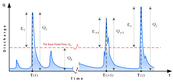
Figure 1.
Hydrograph of the current discharge for the time period studied.
Shane and Lynn [22] proposed the Poisson distribution for modeling the annual number of exceedance and exponential distribution for magnitude estimation. In addition, Pan et al. [23] implied that the Poisson assumption is the most applied technique for the construction of POT data series. The performed studies [18,20,24,25] basically started the peak analysis by using the Poisson distribution and introducing λ (average number of flood peaks) over the threshold (k) within the observed period of time (N).
The aims of the study are given as follows: (a) proposition of the modified exponential distribution taking into account the average number of extreme events for flood estimation; (b) application of the proposed methodology at the long-term hydrological records at the Danube river in Serbia; and (c) benchmarking the proposed method with standard engineering tools (Log-Person III distribution, exponential distribution).
2. Material and Methods
2.1. An Overview of Annual Maximum Series and Peaks-Over-Threshold (POT) Methods
Design flood (DF) provides a better understanding of the differences between the statistical analysis of the annual maximum series and the POT approach. It represents a water stage or discharge to which a water management structure (e.g., top of an embankment, waterfront wall elevation, dam spillway discharge volume, lower elevation of a bridge structure, docklands elevation, etc.) is designed while maintaining its operating stability.
A common practice is to calculate the DF, which is typically defined using the specified return period (e.g., Tp = 100 years, 1000 years), by selecting the maximum from the daily observed series. The minimum recommended number of records is equal to 30, while long-term persistence of the hydrological records implies the use of a longer time period [7]. The sample of annual maximum flood discharge is generated from the recorded time series at the site of the hydrological station. It often happens with large rivers that as much as 20–40% of the annual maximum flood discharges do not even overflow the river banks and extend to inundation areas. The question is whether such a year can be considered within the sample. On the other hand, there can be years with multiple maximum flood discharges exceeding the channel elevation and flooding the surrounding land while only the biggest discharge is taken for analysis. Thus, the relevance of the sample taken from the annual maximum series for the estimation of the DF may be questionable.
The difference between the designed floods estimated from the annual maximum series and the peaks-over-threshold sample is typically reflected in the calculated discharges. This can affect the flow values of designed floods; for instance, the flow values of 100-year and 1000-year flood events. If the sample consists only of floods (peaks-over-threshold sample), then it can be said that the flood of the p = 1% probability is the stage that a river exceeds once in 100 floodings on average. The DF is currently defined (by annual maximum series) as the stage that a river exceeds once in a 100-year period on average.
The above-mentioned two terms for DF determination have been used in hydraulic engineering practice. The difference is that the first approach takes into account only flooding, whereas the latter one also accounts for annual maximum series that do not always represent the flooding event. Those two quantities cannot be considered in an equal manner. Accordingly, the current practice should be reviewed, and the DF is defined as the stage that a river exceeds once in a 100-year period on average. For that reason, a 100-year period taken from an annual maximum series should be considered with caution.
In addition, it can be suggested that long time series of annual maximum series and their related statistical analyses can result in an erroneous conclusion on the safety of a water management structure against a flood peak. Namely, during the last 20–30 years, floods have become more frequent, which is unlikely to affect the output of statistical analyses of long series. In their study, Pan and Rahman [26] illustrate the advantages of using the POT method rather than the annual maximum series for providing a better understanding of the nature of changes in flood events. Even if the annual maximum approach is used in most cases, it cannot represent the complexity of the flood regime [27]. Some authors [28] also suggested the use of annual maximum series for estimation uncertainty in flood frequency analysis. The research of Rosbjerg [15] concludes that the main advantage of the POT method over the annual maximum method is in the short data series case. This is another reason for the current DF determination method to be reviewed.
2.2. Exponential Single-Parameter Distribution
The exponential distribution is widely used in water resource management to estimate the quantiles of both discrete precipitation and flood events. It can be considered as a basic distribution for constructing a number of other distributions representing a type of the two-parameter gamma distribution [29]. It can be easily applied for hydrologic frequency analysis fitting the extreme flood data as a most suitable theoretical distribution [30].
The first step in this research is to select an appropriate distribution function for the time series of extreme discharge where several distribution functions are available. Generally, more than one distribution may fit the data well and select the best model can be difficult [22].
The question is whether the same distribution functions can be used both in the annual maximum analysis and the peaks-over-threshold (POT) analysis or if some other functions, such as one-parameter exponential distributions, should be considered. Namely, because in the peaks-over-threshold analysis, only peak values that lie above a certain truncation level (Xi = Hi − Ho) are considered the coefficient of variation Cv = σ/μ approximates 1.0.
This is shown by Guida et al. [31] in the study of the Tisza River’s maximum annual stages. Moreover, Vukmirović [25] and Todorović [17] used the exponential distribution to estimate quantities of precipitation and discharge, respectively. It is indicated that the advantage of the one-parameter exponential distribution is its simplicity. The gamma distribution is also recommended for a POT analysis by a number of authors [21,32,33,34]. Since the coefficient of variation Cv approximates 1.0, the gamma distribution basically becomes one-parameter exponential distribution [35]. In other words, the one-parameter exponential distribution is a special case of the gamma distribution.
Given that X and Y are variables producing a series of flood peak values and a series of flood durations, respectively, then the following exponential distribution form can be used for peaks over threshold F(x) = P(X < x) [36]:
where α = 1/μ, distribution parameter represents the average value μ = E(X).
A similar form can be written for the Y variable, which describes the duration of the flood above the specified flood stage, G(y) = P(Y < y); thus, the exponential distribution is:
A high degree of correlation noticed between the two series of variables (X, Y) indicates a linear regression between the two. The following can be written for the series of variables (X, Y) H(x,y) = P(X < x, Y < y) using the correlation coefficient :
The next part deals only with the POT analysis since the subject of the paper is the analysis of the DF and not its duration.
Since p(x) = P(X ≥ x) = 1 − F(x), the adopted one-parameter probability distributions can be used to estimate the design flood (xo) of a certain probability of occurrence (exceedance probability) p(xo) = 1% that is, 0.01:
Solving the equation provides:
2.3. Modification of the One-Parameter Exponential Distribution
The advantage of the one-parameter exponential distribution in the estimation of flood records was highlighted in the previous section. However, the one-parameter exponential family does not account for a number of flood events within a specified period of time (λ). A need to introduce a number of flood events is indicated by a number of authors [16,17,34,37].
If we want to analyze the probability of occurrence p(x) and the return period Tp, a number of peaks-over-threshold events within a specified period of time must be introduced. In other words, the following relation may introduce a weighting factor λt:
that is,
A weighting factor λt represents the probability of the number of flood events [38,39,40,41]. The number of flood events certainly also depends on the specified flood stage used to determine flood peaks.
The Poisson distribution is commonly used to estimate the number of exceedances. Given that the probability (p) for a water stage to be above the specified flood stage on a particular day, then (q = 1 − p) is the probability that it will not exceed the specified stage. Therefore, it is suggested that a binominal distribution should be considered, which is indicated by a low (p) and a large number of exceedances. According to the Poisson distribution with variable parameter, the probability of k-exceedances in the time period (0,t) is [42]:
where λt is an average number of exceedances and the λt estimation requires a constant homogenous series of years:
where k is the number of exceedances, and N(t) is the number of years studied.
Considering the above, Equation (2) can also be written in the following form:
where ν indicates the number of exceedances by the series of years.
Assume the event {X > x} labelled with A followed by B = {ν = 0}, = {ν ˃ 0}:
Balancing previous equations generates the following:
If the series of years with exceedances ν expressed by λ follows the Poisson distribution, then: and so that:
Accordingly, the following can be written:
Note that because X < x increases if the years with no exceedances are also accounted for.
The following can be written based on the previous expression:
The above indicates the probability that value X of a flood peak can exceed the specified flood threshold in a particular year. The following designations have been used in solving the equation:
The probability for the event Ā to occur in the year k starting from today is:
As noted, in geometric distribution, the expected time is:
To calculate the value of a flood peak for a particular return period, a 100-year period, for instance, then:
and the solution to the equation is:
that is, the expected value of a stage or a discharge for a particular return period Tp and the exceedance probability (p) with Tp = 1/p is:
where H(Tp) is the estimated stage for a particular return period, H0 is the flood stage (threshold) for flood peaks definition, is the average number of k flood peaks in a specified number of years N(t), is the reciprocal value of the mathematical expectation.
If dealing with discharges, then:
Note that the provided relations are not valid below the threshold specified as a lower boundary value.
2.4. Threshold Selection
The basic assumption for the application of the POT is the existence of the defined threshold values. Based on these values, the maximum flood levels are identified and included for statistical calculation. The threshold values separate the peak values of flood waves from the local maxima and follow the statement that a flood is an overflow of water that submerges land that is in regular conditions, usually dry [35]. From the aforementioned statement, it is suggested that a flood event represents any overflow of the inundation of land caused by the rising river main channel water level (Figure 2). Figure 2 shows a characteristic cross-section of a river stream with a main channel, inundation and embankment.
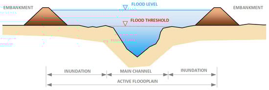
Figure 2.
A characteristic river cross-section with embankments and an active floodplain (main channel and inundation).
The flood threshold value can be expressed in two forms: as a value of the characteristic water level and, alternatively, as a specified value of the water flow [2]. The conclusions of a study conducted by Rasmussen and Rosbjerg [39] implied that there is no unique procedure for selecting a threshold value in POT modeling. This is the main reason for the less frequent use of the POT method [13,23]. The study by Rasmussen and Rosbjerg [38] reviewed several methods and proposed the inclusion of graphical methods and shape stability plots of the generalized Pareto distribution. Durocher et al. [43] developed a semi-automated threshold selection method. Bezak et al. [11] stated that the selection of the threshold value is one of the main disadvantages of the POT method because it is a subjective process.
It is important that the threshold value selected is high enough so that the model assumptions are not violated [24]. The truncation level should be selected as low as possible so that the highest number of exceedances is selected and more reliable parameter estimates can be made [44]. Conclusions of the study conducted by Todorović [37] suggested that the threshold value should be as low as possible, providing that model assumptions are still valid. Ashkar and Rousselle [44] found that if the Poisson and exponential distributions are applicable with a certain threshold, this should remain so with any higher threshold value. Langbein [14] suggested that the base level value should be equal to the lowest series event. This means that at least one event per year is included in the analyses. In their research, Lang et al. [13] suggested some graphical tests that should be used to make the appropriate threshold selection.
The research of Begueria [45] also investigated the influence of threshold selection on partial duration series model assumptions, stating that a unique optimum truncation level cannot be found. In the Flood Estimation Handbook [42], the threshold value is defined so that, on average, one, three or five events per year are selected. On average, four events per year were selected for the Danube River analyses [10]. On the Sava River, it is concluded that a sample of five events per year was selected as optimal [11,45]. It is also suggested that a return period of 1–2 years can be used [46]. The exponential probability distribution function is particularly sensitive to changes in the volume and statistics of the input data series, which affect the shape of the distribution function.
3. Results and Discussion
In this paper, the proposed methodology (Section 2) is applied using the flow time series for Novi Sad hydrological station (Serbia), which drains 254,085 km2 of the Danube River basin. The observed data envelopes the long-term period from 1876 to 2015 [47].
To estimate the flood water levels with the different return periods, the sensitivity of the threshold levels on the flood peak selection has been performed. For this purpose, three water levels have been analyzed as potential flood thresholds (Figure 3). The analyzed values have been transformed into values of the water-level data at the Novi Sad hydrological station. The thresholds are given as follows: 500 cm, 550 cm and 600 cm (Figure 3).
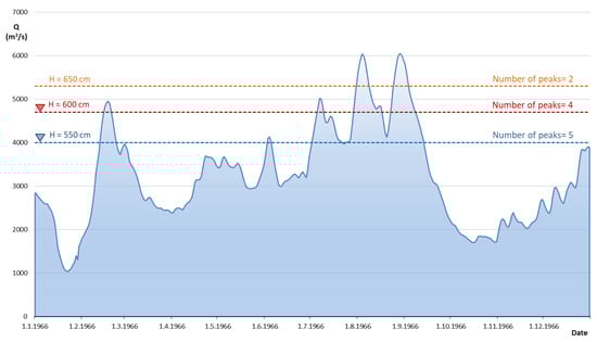
Figure 3.
An example of flood threshold levels and the number of peaks detected for the water levels in 1966 (Dunav river, Novi Sad hydrological station).
Different flood threshold values determine the varying number of flood peaks, which directly affects the theoretical probability distribution parameters. It follows the assumption that the length of the sample directly affects the flood statistics and, consequently, the parameters of the theoretical distribution applied [45].
By increasing the value of the flood threshold level, the number of the selected flood events decreases and directly affects the shape of the exponential probability distribution function (Figure 4). However, Figure 4 implies that for the considered flood threshold levels, the exponential probability distribution function fits very well with the record flood events. In turn, it indicates a good choice of the probability distribution function. The best fit between the theoretical probability distribution and records is achieved for the flood threshold value of H = 550 cm. Therefore, this characteristic threshold is adopted for further analyses.
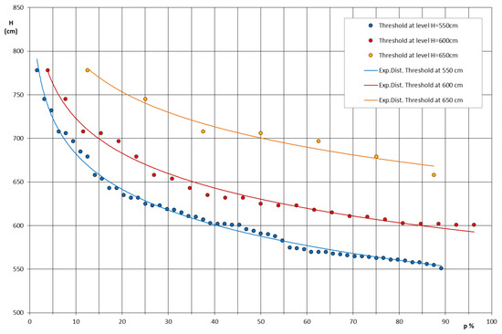
Figure 4.
Exponential probability distribution function dependence of flood threshold level selection.
As the threshold level is selected, the statistical analysis is performed in accordance with the methodology proposed (Section 2.2). The results calculated from the POT analysis with the threshold value of 550 cm are shown alongside the results from the annual maximum series analysis (Figure 5). Please note that the annual maximum series analysis is conducted by the use of HEC-SSP 2.0, which employs the Log-Pearson Type III Distribution alongside the empirical probability distribution, as shown in Figure 5.
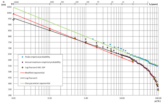
Figure 5.
Comparison of the results from the annual maximum series and POT method above 550 cm at Novi Sad hydrological station.
Note that the results illustrated in Figure 5 implies similar values for extreme water levels; the exceedance probability equals 1%. To be exact, the flood water levels for the Log-Pearson 3 and Modified Exponential Distribution are in line with the following return periods: Tp = 100, 1000 and 10,000 years (Figure 5, black and red lines). However, the modified exponential function with the peaks over threshold analysis suggests somewhat higher water levels (Figure 5, red dots and line) compared to the analysis of the annual maximum series by employing the Log-Pearson Type III Distribution (Figure 5, yellow dots and the black line) with long return periods (Table 1).

Table 1.
Comparison of the results from the selected return periods (1%, 0.1%, 0.01%) of the annual maximum series and POT method above 550 cm at Novi Sad hydrological station.
This proves the statement that the annual maximum series used for the statistical analysis underestimates the water levels with higher return periods since it includes the lower outliers (the years with no floods). Table 1 shows the 1000-year period and the 10,000-year period by 14 cm and 47 cm, respectively, which are higher than the estimation made by using the traditional method of annual maximum series analysis based on the Log-Pearson III distribution. The results (Table 1) obtained by using a one-parameter exponential family are slightly higher compared to the modified one-parameter exponential and Log-Pearson Type III Distribution, which was expected taking into account the approaches described above.
The results of this study are compared with the previous study performed for the Danube river at the river segment in Serbia, Water Management Plan of Serbia (WMPS) [48]. After reviewing the available data from the literature related to flood estimation, it is determined that the nearest hydrological station is Bogojevo hydrological station, located 112 km upstream from the analyzed site (Novi Sad hydrological station).
Due to the fact that there are no significant tributaries between the Danube river segment from the Bogojevo to Novi Sad hydrological stations, the data of flood flows determined for the Bogojevo station is compared with the results from the Novi Sad station. The transformation of the flow values from the Bogojevo hydrological station to the profile of the gauging station Novi Sad has been performed using the Analog catchment method [49]. It determines the transformation coefficient based on the river basin area of the hydrological stations analyzed. The flood flow data, with occurrence probability of p = 1% and 0.1%, has been transformed into water levels using the rating curve for the Novi Sad station [50]. A comparison of the results is shown in Table 2.
Table 2.
Comparison of the results from the WMPS.
The results in Table 2 indicate that the modified exponential distribution slightly overestimates the previous WMPS results [48] for 2.7% and 5.2% in the case of return periods of 1% and 0.1%, respectively. For the case of the standard exponential distributions (one-parameter distribution), results are slightly lower than results in WMPS [48] and range from −4.4 to −0.8% for the return periods analyzed.
4. Conclusions
The paper refers to a common engineering method of flood estimation used for sizing flood control structures on large rivers (e.g., embankments, waterfront walls) but also any other structures along the course of a river (e.g., bridges and docks). The paper provides a detailed procedure for the peaks-over-threshold method with modified one-parameter exponential distribution. The suggested method includes the number of flood events as a distribution parameter for robust estimation of flood water levels.
It is shown that an important parameter that can significantly affect the results in the analysis of the peaks-over-threshold method is the threshold water levels selection. Therefore, sensitivity analysis is performed for several possible threshold water levels (550 cm, 600 cm and 650 cm) at Novi Sad hydrological station (Danube river), and the best matching is achieved for the threshold levels equal to 550 cm. It is concluded that the lower threshold brings the higher sample members and vice versa.
The results of the performed analysis at Novi Sad hydrological station indicate that the modified and standard one-parameter distributions estimate water levels for return periods of 1000 years equal to 867 cm and 922 cm, respectively. On the other hand, the Log-Pearson III distribution using the annual extremes underestimates the water levels with the same return periods in the range from 1.6% to 8%. It can be attributed to the fact that the annual extremes envelop the same lower values of flood events, which can not be considered as a flooding event. Moreover, the POT method takes into account only the flood values above the defined threshold (550 cm) as they represent realistic flooding events.
The results derived from the previous study (WMPS) are also used to verify the flood estimates from the POT method under the modified one-parameter exponential distribution at Novi Sad hydrological station. For comparison purposes, the Bogojevo hydrological station located at the Danube river in Serbia is used. It can be concluded that the results from the previous study slightly underestimate the flood water levels for 2.7% and 5.2% in the case of 100 and 1000 years return periods, respectively.
It can be concluded that the issue of a flooded threshold requires detailed consideration and suggests specifying the adequate threshold level. As it is mentioned, the main advantage of the POT method and modified one-parameter exponential distribution is the realistic samples for flood estimation that envelope only the data considered as a flooding event. On the other hand, the limitation of the wider application of the POT method is its completion, mainly because of the time-consuming process needed for the threshold selection. However, the POT method, alongside the modified one-parameter distribution, better fits the measured data and provides a visible alternative for flood design estimation.
Further works related to the proposed approach have several directions: application of the proposed methodology at the sites of international rivers in Serbia (e.g., Danube, Sava and Tisza) and comparison of the results to the traditional approach; its application on the hydrological stations at the Danube river under the influence of the Iron 1 gate hydro-energy system [51], where the realistic records are only water levels rather than estimated flows.
Supplementary Materials
Authors support the open scientific exchange of data and results. The research data are available in a publicly accessible repository: https://doi.org/10.5281/zenodo.7742318.
Author Contributions
Conceptualization, S.K. (Srđan Kolaković) and D.S.; methodology, S.K. (Srđan Kolaković) and G.J.; formal analysis, S.K. (Slobodan Kolaković); investigation, S.K. (Slobodan Kolaković), V.M. and M.S.; writing—original draft preparation, S.K. (Slobodan Kolaković); and editing, M.S. and V.M. All authors have read and agreed to the published version of the manuscript.
Funding
This research received no external funding.
Institutional Review Board Statement
Not applicable.
Informed Consent Statement
Not applicable.
Data Availability Statement
Data is contained within the supplementary material.
Acknowledgments
This study has been supported by the Republic of Serbia, Ministry of Education, Science and Technological Development through project number 451-03-47/2023-01/200108. The research has been conducted within the project “Scientific theoretical and experimental research and improvement of educational process in the field of civil engineering”, developed at the Department of Civil Engineering and Geodesy, Faculty of Technical Sciences, University of Novi Sad, Sebia.
Conflicts of Interest
The authors declare no conflict of interest.
References
- Stojković, M.; Kostić, S.; Prohaska, S.; Plavšić, J.; Tripković, V. A New Approach for Trend Assessment of Annual Streamflows: A Case Study of Hydropower Plants in Serbia. Water Resour. Manag. 2017, 31, 1089–1103. [Google Scholar] [CrossRef]
- Bonacci, O.; Ljubenkov, I. Changes in flow conveyance and implication for flood protection, Sava River, Zagreb. Hydrol. Process. 2008, 22, 1189–1196. [Google Scholar] [CrossRef]
- Tavares, L.V.; Da Silva, J.E. Partial duration series method revisited. J. Hydrol. 1983, 64, 1–14. [Google Scholar] [CrossRef]
- Brilly, M.; Polic, M. Public perception of flood risks, flood forecasting and mitigation. Nat. Hazards Earth Syst. Sci. 2005, 5, 345–355. [Google Scholar] [CrossRef]
- Mikoš, M.; Brilly, M.; Ribičič, M. Floods and Landslides in Slovenia. Acta Hydrotech. 2004, 22, 113–133. [Google Scholar]
- Djoric, D.; Malisic, J.; Jevremovic, V.; Nikolic-Djoric, E. Atlas Raspodela; Građevinski Fakultet Univerziteta u Beogradu: Beograd, Serbia, 2007; ISBN 978-86-7518-077-7. [Google Scholar]
- Stojković, M.; Prohaska, S.; Zlatanović, N. Estimation of flood frequencies from data sets with outliers using mixed distribution functions. J. Appl. Stat. 2017, 44, 2017–2035. [Google Scholar] [CrossRef]
- Mays, L.W. Water Resources Engineering; John Wiley & Sons: Hoboken, NJ, USA, 2010; ISBN 978-0-470-57416-4. [Google Scholar]
- Council of the European Communities. Directive 2007/60/EC of the European Parliament and of the Council of 23 October 2007 on the assessment and management of flood risks. Off. J. Eur. Communities 2007, 288, 27–34. [Google Scholar]
- Bačová-Mitková, V.; Onderka, M. Analysis of extreme hydrological events on the Danube using the Peak Over Threshold method. J. Hydrol. Hydromech. 2010, 58, 88–101. [Google Scholar] [CrossRef]
- Bezak, N.; Brilly, M.; Šraj, M. Comparison between the peaks-over-threshold method and the annual maximum method for flood frequency analysis. Hydrol. Sci. J. 2014, 59, 959–977. [Google Scholar] [CrossRef]
- Gottschalk, L.; Krasovskaia, I. L-moment estimation using annual maximum (AM) and peak over threshold (POT) series in regional analysis of flood frequencies. Nor. Geogr. Tidsskr.-Nor. J. Geogr. 2002, 56, 179–187. [Google Scholar] [CrossRef]
- Lang, M.; Ouarda, T.B.M.J.; Bobée, B. Towards operational guidelines for over-threshold modeling. J. Hydrol. 1999, 225, 103–117. [Google Scholar] [CrossRef]
- Langbein, W.B. Annual floods and the partial-duration flood series. Trans. Am. Geophys. Union 1949, 30, 879–881. [Google Scholar] [CrossRef]
- Rosbjerg, D. Estimation in partial duration series with independent and dependent peak values. J. Hydrol. 1985, 76, 183–195. [Google Scholar] [CrossRef]
- Todorovic, P.; Rousselle, J. Some Problems of Flood Analysis. Water Resour. Res. 1971, 7, 1144–1150. [Google Scholar] [CrossRef]
- Todorovic, P.; Woolhiser, D.A. On the time when the extreme flood occurs. Water Resour. Res. 1972, 8, 1433–1438. [Google Scholar] [CrossRef]
- Todorovic, P.; Zelenhasic, E. A Stochastic Model for Flood Analysis. Water Resour. Res. 1970, 6, 1641–1648. [Google Scholar] [CrossRef]
- International Commission for Protection of the Danube River Basin (ICPDR) Floods and Flood Risk Management. Available online: https://www.icpdr.org/main/issues/floods (accessed on 2 March 2023).
- Burn, D.H.; Whitfield, P.H. Changes in cold region flood regimes inferred from long-record reference gauging stations. Water Resour. Res. 2017, 53, 2643–2658. [Google Scholar] [CrossRef]
- Li, Y.; Saxena, K.M.L.; Cong, S. Estimation of the extreme flow distributions by stochastic models. Extremes 1999, 1, 423–448. [Google Scholar] [CrossRef]
- Shane, R.M.; Lynn, W.R. Mathematical Model for Flood Risk Evaluation. J. Hydraul. Div. 1964, 90, 1–20. [Google Scholar] [CrossRef]
- Pan, X.; Rahman, A.; Haddad, K.; Ouarda, T.B.M.J. Peaks-over-threshold model in flood frequency analysis: A scoping review. Stoch. Environ. Res. Risk Assess. 2022, 36, 2419–2435. [Google Scholar] [CrossRef]
- Kjeldsen, T.R.; Lundorf, A.; Rosbjerg, D. Use of a two-component exponential distribution in partial duration modelling of hydrological droughts in Zimbabwean rivers. Hydrol. Sci. J. 2000, 45, 285–298. [Google Scholar] [CrossRef]
- Vukmirović, V. Analiza kiše metodom parcijalnih serija. Vodoprivreda 2010, 42, 243–245. [Google Scholar]
- Pan, X.; Rahman, A. Comparison of annual maximum and peaks-over-threshold methods in flood frequency analysis’. In Proceedings of the Hydrology and Water Resources Symposium (HWRS 2018): Water and Communities, Melbourne, Australia, 3–6 December 2018; Engineers Australia Melbourne: Melbourne, Australia, 2018; p. 614. [Google Scholar]
- Burn, D.H.; Whitfield, P.H. Changes in flood events inferred from centennial length streamflow data records. Adv. Water Resour. 2018, 121, 333–349. [Google Scholar] [CrossRef]
- Karim, F.; Hasan, M.; Marvanek, S. Evaluating Annual Maximum and Partial Duration Series for Estimating Frequency of Small Magnitude Floods. Water 2017, 9, 481. [Google Scholar] [CrossRef]
- Singh, V.P. Exponential Distribution. In Entropy-Based Parameter Estimation in Hydrology; Springer: Dordrecht, The Netherlands, 1998; pp. 49–55. [Google Scholar]
- Mohsen, S.; Zulkifli, Y.; Fadhilah, Y. Modeling the Distributions of Flood Characteristics for a Tropical River Basin. J. Environ. Sci. Technol. 2012, 5, 419–429. [Google Scholar] [CrossRef]
- Guida, R.J.; Swanson, T.L.; Remo, J.W.F.; Kiss, T. Strategic floodplain reconnection for the Lower Tisza River, Hungary: Opportunities for flood-height reduction and floodplain-wetland reconnection. J. Hydrol. 2015, 521, 274–285. [Google Scholar] [CrossRef]
- Buishand, T.A. Some remarks on the use of daily rainfall models. J. Hydrol. 1978, 36, 295–308. [Google Scholar] [CrossRef]
- Fraser, D.A.S. Nonparametric Methods in Statistics; John Wiley & Sons Inc.: Hoboken, NJ, USA, 1956. [Google Scholar]
- Zelenhasic, E.F. Theoretical Probability Distributions for Flood Peaks. Ph.D. Thesis, Colorado State University, Denver, CO, USA, 1970. [Google Scholar]
- Maidment, D.R. Handbook of Hydrology; McGraw-Hill: New York, NY, USA, 1993; ISBN 978-0070397323. [Google Scholar]
- Barabás, B.; Kovács, S.; Reimann, J. Növekednek-e az árvizek? (Rising floods?). J. HUNGARIAN Hydrol. Soc.-Hidrológiai Közlöny 2004, 84, 1–7. [Google Scholar]
- Todorovic, P. Stochastic models of floods. Water Resour. Res. 1978, 14, 345–356. [Google Scholar] [CrossRef]
- Rasmussen, P.F.; Rosbjerg, D. Risk estimation in partial duration series. Water Resour. Res. 1989, 25, 2319–2330. [Google Scholar] [CrossRef]
- Rasmussen, P.F.; Rosbjerg, D. Prediction Uncertainty in Seasonal Partial Duration Series. Water Resour. Res. 1991, 27, 2875–2883. [Google Scholar] [CrossRef]
- Salas, J.D.; Heo, J.H.; Lee, D.J.; Burlando, P. Quantifying the Uncertainty of Return Period and Risk in Hydrologic Design. J. Hydrol. Eng. 2013, 18, 518–526. [Google Scholar] [CrossRef]
- Willkofer, F.; Wood, R.R.; von Trentini, F.; Weismüller, J.; Poschlod, B.; Ludwig, R. A Holistic Modelling Approach for the Estimation of Return Levels of Peak Flows in Bavaria. Water 2020, 12, 2349. [Google Scholar] [CrossRef]
- Reed, D.; Robson, A. Flood Estimation Handbook; Institute of Hydrology Wallingford: Wallingford, UK, 1999; Volume 3, ISBN 9781906698003. [Google Scholar]
- Durocher, M.; Mostofi Zadeh, S.; Burn, D.H.; Ashkar, F. Comparison of automatic procedures for selecting flood peaks over threshold based on goodness-of-fit tests. Hydrol. Process. 2018, 32, 2874–2887. [Google Scholar] [CrossRef]
- Ashkar, F.; Rousselle, J. Partial duration series modeling under the assumption of a Poissonian flood count. J. Hydrol. 1987, 90, 135–144. [Google Scholar] [CrossRef]
- Beguería, S. Uncertainties in partial duration series modelling of extremes related to the choice of the threshold value. J. Hydrol. 2005, 303, 215–230. [Google Scholar] [CrossRef]
- Irvine, K.N.; Waylen, P.R. Partial Series Analysis of High Flows in Canadian Rivers. Can. Water Resour. J. 1986, 11, 83–91. [Google Scholar] [CrossRef]
- IPA European Union. IPA Project HU-SRB/0901/121/0—TRMODELL. 2013. Available online: https://keep.eu/projects/6461/Tisza-River-Modelling-on-the-EN/ (accessed on 2 March 2023).
- Dimkić, M.; Dacić, M.; Prohaska, S.; Babić Mladenović, M.; Stevanović, S. Water Management Plan of Serbia; Srbijavode: Belgrade, Serbia, 2009. [Google Scholar]
- Ben Daoud, A.; Sauquet, E.; Bontron, G.; Obled, C.; Lang, M. Daily quantitative precipitation forecasts based on the analogue method: Improvements and application to a French large river basin. Atmos. Res. 2016, 169, 147–159. [Google Scholar] [CrossRef]
- Milašinović, M.; Prodanović, D.; Zindović, B. Rekonstrukcija hidrograma na vodomernim stanicama primenom rezultata asimilacije preliminarni rezultati. In Proceedings of the Zbornik Radova 19. Naučnog Savetovanja Srpskog Društva za Hidraulička Istraživanja i Srpskog Društva za Hidrologiju, Belgrade, Serbia, 18–19 October 2021; Univerzitet u Beogradu–Građevinski Fakultet: Beograd, Serbia, 2021; pp. 255–265. [Google Scholar]
- Divac, D.; Grujović, N.; Milivojević, N.; Stojanović, Z.; Simić, Z. Hydro-information systems and management of hydropower resources in Serbia. J. Serb. Soc. Comput. Mech. 2009, 3, 1–37. [Google Scholar]
Disclaimer/Publisher’s Note: The statements, opinions and data contained in all publications are solely those of the individual author(s) and contributor(s) and not of MDPI and/or the editor(s). MDPI and/or the editor(s) disclaim responsibility for any injury to people or property resulting from any ideas, methods, instructions or products referred to in the content. |
© 2023 by the authors. Licensee MDPI, Basel, Switzerland. This article is an open access article distributed under the terms and conditions of the Creative Commons Attribution (CC BY) license (https://creativecommons.org/licenses/by/4.0/).