Performance Comparison of Deep Learning Approaches in Predicting EV Charging Demand

Abstract

Electric vehicles (EVs) contribute to reducing fossil fuel dependence and environmental pollution problems. However, due to complex charging behaviors and the high demand for charging, EVs have imposed significant burdens on power systems. By providing reliable forecasts of electric vehicle charging loads to power systems, these issues can be addressed efficiently to dispatch energy. Machine learning techniques have been demonstrated to be effective in forecasting loads. This research applies six machine learning methods to predict the charging demand for EVs: RNN, LSTM, Bi-LSTM, GRU, CNN, and transformers. A dataset containing five years of charging events collected from 25 public charging stations in Boulder, Colorado, USA, is used to validate this approach. Compared to other highly applied machine learning models, the transformer method outperforms others in predicting charging demand, demonstrating its ability for time series forecasting problems.

1. Introduction

The electric vehicle industry has captured the attention of governments, automakers, and energy companies. There is a growing consensus that electric vehicles are a viable solution to dwindling fossil fuel resources and increasing pollution. The popularity of EVs has been widely credited with reducing greenhouse gas emissions (mainly carbon dioxide) [1,2].

An anticipated large-scale EV rollout will pose both a challenge and an opportunity for power systems. The simultaneous charging of many electric vehicles could cause severe bottlenecks in distribution systems, requiring costly upgrades to grids [3,4,5]. Consequently, utilities and other power generators should prepare for increased loads as the electrification of the transportation system grows. Considering that load forecasting is a key component of power utility operations, decision-makers should be able to forecast future electricity demand with a minimum error percentage. In the case of utility companies, accurate load predictions can result in significant savings [6].

There are three charging station categories based on the charger type (Levels 1 through 3). Charging stations can also be divided into home, workplace, and commercial charging stations [7]. Most homes and workplaces have Level 1 and 2 plugs to accommodate electric vehicle charging during the night or work hours. Commercial stations, on the other hand, use Level 2 and Level 3 plugs to satisfy the more urgent needs of electric vehicle drivers [8].

Table 1. EV charging level description.

Level	Power Level	Power Limit (kW)	Charging Speed	Charging Time (h)
Level 1 AC	110/120 VAC	≤3.3	Slow	4–36
Level 2 AC	208/240 VAC	3.3–20	Medium	1–4
Level 3 (DC fast charging)	440 or 480 VAC	>50	Fast	0.2–1

describes the three general levels of charging infrastructure that are commercially available. Level 1 AC (alternating current) chargers are the slowest charging levels and can be used to charge most PHEVs overnight or at workplaces. However, an empty AEV may require more than one night of charging. Compared to Level 1 AC, Level 2 AC draws more current and runs at a higher voltage, allowing it to charge faster. Typically, Level 2 AC systems can fully charge an AEV from empty overnight, which is why they are often recommended for installation in the residences of owners of AEVs. For daytime charging, Level 2 AC chargers are commonly installed in areas where vehicles are parked for a short period. Chargers that operate as a Level 1 DC (direct current) or a Level 2 DC (direct current) are the fastest chargers. Most AEVs can be charged to 80 percent capacity with a Level 2 DC charger within 20 min, except during extreme temperatures [9].

Commercial charging stations differ significantly from home/workplace charging stations because their charging patterns are less predictable than those at homes/workplaces due to trip purposes, weather, driver accessibility, and other miscellaneous factors. However, it is more pertinent and useful for agencies to forecast the charging demand at commercial charging stations to plan for charging infrastructure. For one thing, fast charging stations have high voltage requirements. Power grid reliability and robustness can be enhanced by the accurate prediction of charging demand. Secondly, forecasting the distribution of charging demand across spatiotemporal dimensions can be helpful for both manufacturers and users of electric vehicles in planning future charging infrastructure [10].

Predicting the charging demand for electric vehicles is the basis for researching the impact of charging EVs on an electricity grid. The accuracy of EV charging forecasts is essential for utility decision-making and development. Besides providing solutions for charging station construction planning, increasing the prediction precision for optimal dispatching, and providing manufacturers with strong incentives for EV adoption, accurate predictions also provide the basis for research on electric vehicle charging strategies. Several unique techniques have been developed for monitoring EV charging, and many methods have been identified for modeling EV charging demand as a result of previous research [11].

This study applies deep learning methods to forecast EV charging loads using real-world charging records collected in Denver, Colorado, to provide real-time forecasts. The remaining sections of this paper are structured as follows: Section 2 provides a detailed review of related works in the literature in this field, and it provides a rationale for this research. Section 3 describes the proposed predictive models and the datasets used in this study. Section 4 presents the simulation results and a discussion about the attained solution. Finally, Section 5 provides the study’s conclusion.

2. Literature Review

Over the past few decades, researchers have developed various modules for improving the accuracy of different load forecasting methods, either by using traditional methods or by utilizing Artificial Intelligence (AI). Intelligent algorithms have contributed to the success of big data technologies in many applications due to the rapid development of Artificial Intelligence, deep learning, and machine learning (ML) [6].

An overview of the current state of the art in EV charging load forecasting is presented in this section to identify the limitations of previous research and highlight the contributions of this study.

Deep Learning Models

The concept of deep learning was first defined by Hinton et al. in 2006 as a result of their study on artificial neural networks (ANN) [12]. A multilayer perceptron was used to represent the structure of deep learning by combining low-level features to form higher-level abstractions of attribute categories or features and discovering distributed feature representations of the data. Deep learning models possess the excellent generalization and learning capabilities required to be competitive in complex forecasting tasks.

The study by Kumar et al. demonstrated the application of ANN algorithms in forecasting the EV charging load on a distribution system. Three neural networks—ANN, R-ANN, and RR-ANN—were used to estimate the 24 h charging profiles based on travel behaviors. The results showed that the RR-ANN model outperformed the other models, achieving the highest accuracy [13].

Research on EV forecasting is frequently carried out using recurrent neural networks (RNNs) and long short-term memories (LSTMs) as variations of ANNs. Sequence data can be processed effectively with RNN models. Among other applications, they have been successfully used in natural language processing, machine translation, and time-series predictions [14]. Using recurrent neural networks (RNNs), Vermaak and Botha developed a short-term load forecasting model for the first time [15]. In the standard RNN training process, gradient issues such as gradient disappearing and exploding are encountered. Several variant structures, such as short-term memories (LSTMs), GRUs, and convolutional neural networks (CNNs), have been proposed to overcome these issues in recent years.

Marino et al. applied the LSTM model to predict building energy loads using the number of neuron nodes in the model [16]. Based on the results of a study conducted by Kong et al. on forecasting residential loads using an LSTM algorithm, the LSTM showed the most remarkable performance [17]. Similarly, Lu et al. studied neural networks for predicting the EV load aggregated hourly. According to the back-testing results, the LSTM model performed better than other neural networks [18]. As demonstrated in an article by Zhu et al., an LSTM delivered a superior performance in forecasting EV loads. The study developed an LSTM for single-step predictions. As a result of the analysis, the LSTM outperformed a simple ANN for a forecast horizon of 15 and 30 min, and that prediction error diminished as the forecast horizon decreased [19]. Another LSTM forecasting method was presented in a study by Gao et al. [20]. This study examined four EV types—private and commercial EVs, electric buses, and electric taxis. Based on MCS, the LSTMs outperformed the backpropagation networks (BP) and SVRs.

Zheng et al. predicted the electric load profiles of a building for each 15-min interval using an LSTM neural network [21]. In addition, an LSTM model with a pooling technique was presented to forecast individual residential loads [22]. Chang et al. evaluated the performance of an LSTM-based approach in predicting the aggregated charging power demand in multiple fast-charging stations in Jeju, Korea. Compared with other deep learning models, their LSTM model demonstrated the highest accuracy and performance [23].

Using deep learning approaches, Zhu et al. predicted short-term charging station loads. The study examined four deep learning models: deep neural networks, standard RNNs, LSTMs, and GRUs. The authors used the charging load sequence from the preceding 24 h period to predict the charging load for the next hour. According to the results, the GRU produced the best results compared to the other three models [24].

In several fields of study, bidirectional LSTMs (Bi-LSTMs) have provided accurate aggregated power load forecasts [17,25]. A study published by Mohsenimanesh et al. assessed the effectiveness of three deep learning algorithms in forecasting the aggregate load for charging a fleet of electric cars, namely, an LSTM, a Bi-LSTM, and a GRU. A real-world dataset of 1000 electric vehicles was collected in Canada between 2017 and 2019. The models developed were trained and tested using this dataset. In the study, the Bi-LSTM had the lowest mean absolute error, mean absolute percentage error, and root mean square error, making it the optimal method for forecasting electric car fleet loads [26]. According to Di Persio et al., EV charging forecasting was performed using several variations of standard LSTMs, including a multilayer LSTM, a bi-LSTM, and sequence-to-sequence LSTMs. Based on the results, Bi-LSTM outperformed the other methods for that specific time series load [27].

Recently, CNN models have gained popularity in time series forecasting. Research by Sadaei et al. combined fuzzy time series (FTS) with a CNN to forecast short-term loads [28]. Using NILA in combination with a CNN, Li et al. presented a hybrid model for predicting short-term EV charging station loads. A NILA-CNN model was found to be effective in predicting EV charging station loads, beating other models in terms of accuracy [29].

According to the literature review, RNNs, LSTMs, Bi-LSTMs, and CNNs have all been successfully used to forecast EV loads. Furthermore, these methods are subject to several limitations due to their sequential processing of the input data, especially when dealing with datasets with long dependencies [30]. A transformer-based solution has been developed to deal with the issue of long-term dependencies in time series forecasting.

Transformers are machine learning models that utilize scaled dot product operations or self-attention as their principal training mechanism [31]. There have been numerous applications of transformers, and they have been applied to a variety of problems in machine learning, such as natural language processing (NLP), speed recognition, and motion analysis, with state-of-the-art performance [32,33,34]. Attention mechanisms have also recently gained popularity in time series forecasting tasks.

The transformer model has been used effectively in previous studies for EV load forecasting, as seen in [35]. However, this study sought to build upon previous works by incorporating six deep learning models—RNNs, LSTMs, Bi-LSTMs, GRUs, CNNs, and transformers—to compare these models’ performances comprehensively. The goal was to identify the best-performing model for EV charging load forecasting to improve the accuracy of predictions. The key contributions of this study are:

1. This study utilized three different time steps to predict the charging load for EVs. The datasets used were based on daily, weekly, and monthly data. As the data were aggregated into weekly and monthly intervals, data noise was reduced, and a smoother dataset was produced. Moreover, the dataset can be used to simulate and train models based on limited data. Testing models based on limited data is crucial for ensuring their robustness and reliability. This information can help energy companies and planners make informed decisions on energy supply and demand management.

2. This study aimed to comprehensively evaluate the potential of deep learning approaches for predicting electric vehicle (EV) charging loads. Six deep learning models were employed to achieve this objective, including both widely applied methods and hybrid models. The results obtained in this study provide valuable insights and have been compared to existing literature in this field, contributing to the advancement of knowledge in this area. Through this comprehensive comparison, the study addressed the current limitations in using deep learning models for EV charging load predictions.

This paper used deep learning to forecast the charging demand for electric vehicles in Denver, Colorado. A dataset consisting of 436,000 observations of charging events collected from 25 public charging stations in Colorado was used to apply the mentioned deep learning models. This study used three different datasets by aggregating EV charging loads into daily, weekly, and monthly datasets, and then it forecast the demand for the next time step in each dataset. The performance and accuracy of the six prediction algorithms were evaluated using the root mean square error (RMSE) and mean absolute error (MAE) metrics.

3. Materials and Methods

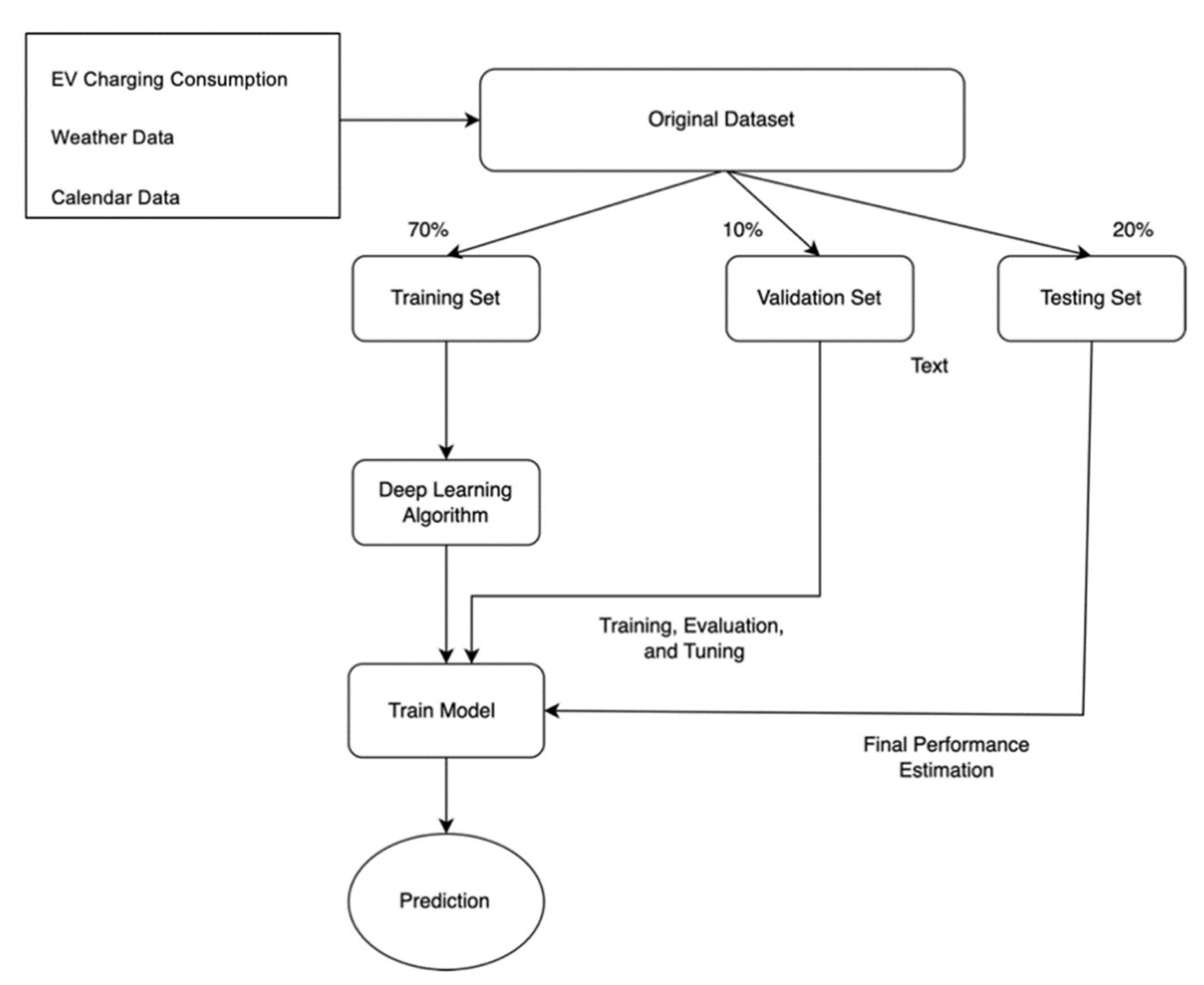
3.1. Charging Demand Prediction Framework

In this research, we assessed the feasibility of predicting the energy consumption of electric vehicles at public charging stations in a regulated electricity market by using actual data and deep learning algorithms based on the energy consumption of 25 public charging stations in Boulder, Colorado.

Various regression methods have been tested and proven over the years, each with its benefits and shortcomings. The present paper aimed to investigate the performance of six deep learning algorithms, namely, recurrent neural networks (RNNs), long short-term memories (LSTMs), bidimensional LSTMs (Bi-LSTMs), gated redcurrant units (GRUs), convolutional neural networks (CNNs), and transformers. Figure 1 illustrates the overall framework of the deep learning approaches. Section 3.1.1 through Section 3.1.6 present the deep learning approaches considered in this study.

3.1.1. Recurrent Neural Networks (RNNs)

An artificial neural network (ANN) contains multiple layers of interconnected neurons. In neural networks, input layers accept input values, hidden layers transform those values, and output layers produce output values. The layers are connected by weights. There are many classes of ANNs which can be used for many different purposes [36]. A recurrent neural networks (RNNs) is a specific class of ANN. A recurrent neural network has recurrent connections, which means that its current output also depends on its previous output; more specifically, it memorizes its previous output and uses it to calculate its current output. Figure 2 shows the RNN structure.

Mathematically, for time t, the RNN formula is:

$$S_t=f \left(W{S}_{t-1}+U{x}_t+b\right) \mathrm{and}$$

(1)

$$O_t=g \left(V{S}_t\right),$$

(2)

where f and g are the nonlinear activation functions (sigmoid functions), $S_t$ and $x_t$ represent the hidden layer and input layer, respectively, in the time step $t$, and $W$, $U$, and $V$ represent weight matrices. $O_t$ represents the output and b represents the bias.

3.1.2. Long Short-Term Memory (LSTM)

Horchreiter and Schmidhuber proposed long short-term memory (LSTM) in 1997 to overcome vanishing or expanding gradients. The LSTM structure is shown in Figure 3 [37]. In LSTM networks, such problems are addressed by integrating specific gate mechanisms into the recurrent feedback loops. Neuronal networks’ gate mechanisms decide which information should be retained or discarded during the learning process. An LSTM has three gated cell memories in its internal structure—an input gate ($i$) which identifies and permits new inputs, a forget gate ($f$) that obliterates irrelevant data, and an output gate ($o$) which determines the final output based on the current state. In an LSTM, memory is configured as gated cells which decide whether to store or delete data from the network model. Gated cells make decisions based on weight coefficients and weight changes during progressive training. As the training process proceeds, the information with the highest significance will be retained in the LSTM memory and the rest will be removed.

The formulation of updating the cell states and parameters is expressed as follows:

$$f_t=\sigma \left(x_t{U}^f+h_{t-1}{W}^f\right),$$

(3)

$$i_t=\sigma \left(x_t{U}^i+h_{t-1}{W}^i\right),$$

(4)

$${\tilde{C}}_t=\mathit{tanh}\left(x_t{U}^g+h_{t-1}{W}^g\right),$$

(5)

$$C_t=\sigma \left(f_t\times C_{t-1}+i_t\times {\tilde{C}}_t\right), \mathrm{and}$$

(6)

$$h_t=\tanh \left(C_t\right)\times o_t,$$

(7)

where $i_t$, $f_t$, and $o_t$ are the input gate, forget gate, and output gate, respectively, at time $t$, $x_t$ is the input data at the time step $t$, and $h_{t-1}$ stands for the hidden layer in time $t$. $C_{t-1}$ and $C_t$ are cell states for the times $t-1$ and $t$, respectively, and ${\tilde{C}}_t$ is the internal memory unit. $W$ and $U$ denote the weight matrices associated with the corresponding gates.

3.1.3. Bidimensional LSTM (Bi-LSTM)

An extension of the described LSTM models is the Bi-LSTM model, which has two LSTM units that work in both directions to incorporate past and future information [38]. In the first round, the forward-moving LSTM receives the past data from input sequences, and in the second round, the backward-moving LSTM receives the future data. The structure of a Bi-LSTM model is shown in Figure 4.

In Bi-LSTM, the hidden layer contains both forward and backward tensors. The backward hidden state and forward hidden state at the time step t are shown as $\overrightarrow{h_t}$ and $\overleftarrow{h_{t }}$, respectively. For a hidden state at a specific time, step t is fed into the output layer, which is obtained by concatenating the forward and backward hidden states as follows:

$$h_t=\left[\overrightarrow{h_t}, \overleftarrow{h_t}\right]$$

(8)

3.1.4. Gated Recurrent Unit (GRU)

A gated recurrent unit (GRU) is a time-efficient and rich improvement to an LSTM that simplifies the LSTM’s structure and improves the design of its gates. In a GRU model, the LSTM input gate is combined with the forget gate into one update gate, and the LSTM output gate is designated as a reset gate [39]. Figure 5 illustrates the overall structure of a GRU.

The update gate ($z_t$) is responsible for determining how much past knowledge needs to be passed on to future generations. The update gate of a GRU is analogous to the output gate of an LSTM. The reset gate ($r_t$) determines how much previous knowledge should be forgotten. It is equivalent to combining the input and forget gates in an LSTM recurrent unit [40].

$$z_t=\sigma \left(x_t{W}_z+h_{t-1}{U}_z\right)$$

(9)

$$r_t=\sigma \left(x_t{W}_r+h_{t-1}{U}_z\right)$$

(10)

$${\tilde{h}}_t=\mathit{tanh}\left(x_t{W}_h+r_t\times U_h h_{t-1}\right)$$

(11)

$$h_t=z_t\times h_{t-1}+\left(1-z\right)\times {\tilde{h}}_t$$

(12)

In the GRU formula, $z_t$ and $r_t$ are the update gate and reset gate, respectively, at time $t$. $x_t$ stands for the input data at the time step $t$, and $h_t$ represents the hidden layer in the time step $t$. ${\tilde{h}}_t$ is the candidate activation, and $W$ and $U$ are the weight matrices associated with the corresponding gates.

3.1.5. Convolutional Neural Networks (CNNs)

A convolutional neural network (CNN) is an artificial neural network initially developed for processing image data and language processing applications [41]. Figure 6 shows a 1D CNN structure for a time-series forecasting model. It consists of an input layer, a convolutional layer, a pooling layer, a flattened layer, a fully connected layer, and an output layer. As can be seen in Figure 6, either the convolution layer or the pooling layer is constructed of artificial neurons representing convolutional filters.

The convolutional layer reads the input and applies convolutional filtering to extract potential features. The pooling layer is used to reduce the input representation’s spatial size and parameter count. A fully connected layer maps the features extracted by the network to classes or values.

3.1.6. Transformers

Using a mechanism inspired by human perception, transformer models can improve time series forecasting accuracy by selectively focusing on certain input data and ignoring others. In 2017, Vaswani et al. published the first transformer architecture [31]. This architecture implemented self-attention, eliminating the need for recurrent neural networks [42].

In general, attention is best utilized by capturing the most essential information from large amounts of data. Transformers do not suffer from vanishing gradients and are capable of accessing any point in the past, regardless of how far back the time steps go. Through this feature, a transformer can detect long-term dependencies.

Figure 7 shows the general architecture of a transformer model. A transformer uses encoder-decoder structures containing stacked encoder and decoder layers. As shown in Figure 7, the encoder layer has two sublayers: the first is the multi-head self-attention mechanism and the second is the feed forward mechanism. Similarly, the decoder layer can be deconstructed into three sub-layers. Decoding is based on three sublayers: multi-head attention, masked multi-head attention, and feed-forward mechanisms. With multi-head attention, all subsequent positions are excluded from the predictor input. Layer normalization is followed by residual connections surrounding each sublayer, which speeds up the training speed and convergence.

Using the encoder, time series data is received as sequential sequences ($x_1$,..., $x_n$) which are converted into continuous representations ($z_1$,..., $z_n$). Based on $z$, the decoder calculates the output and then generates one symbol at a time ($y_1$,..., $y_m$). A transformer is an auto-regressive model that uses previous symbols as additional inputs. The output layer $y_i$ at the time step $i$ is written as:

$$y_i={\sum }_{j=1}^n{a}_{ij}\left(x_j{W}_V\right),$$

(13)

where $y_i$ is the updated $x_j$ and $a_{ij}$ is the attention score that measures the similarity between $x_i$ and $x_j$. $a_{ij}$ is calculated as:

$$a_{ij}=\frac{\exp \left(e_{ij}\right)}{{\sum }_{k=1}^n\exp \left(e_{ik}\right)},$$

(14)

where $e_{ij}$ measures the combability of two linearly transformed input elements, $x_i$ and $x_j$, and it is calculated as:

$$e_{ij}=\frac{(x_i{W}_Q){(x_j{W}_K)}^T}{\sqrt{h}}$$

(15)

In this formula, $W_K, W_Q,$ and $W_K$ are three linear transformation matrices that increase the transformer’s expressiveness, and $h$ is the dimension of the model. Figure 7 shows the structure of a transformer.

Table 2. Differences between the deep learning approaches.

Model	Key Characteristics
RNN	Sequential data is processed by passing hidden states from one step to another, allowing dependencies to be captured between them [36].
LSTM	An LSTM is an extension of an RNN and consists of memory cells and gates to control information flow and avoid the vanishing gradients problem. It is capable of capturing long-term relationships [37].
Bi-LSTM	A bidirectional version of LSTM, bi-LSTM processes a sequence in two directions and combines the results, capturing dependencies both previously and in the future [38].
GRU	As a variation of an RNN, a GRU incorporates two gates (update and reset gate) that control the information flow, improving convergence compared to traditional RNNs [39].
CNN	A CNN is designed to process grid-structured data (e.g., images) by combining local features extracted from the input with convolutional layers [41].
Transformer	A transformer uses self-attention mechanisms to process sequential data, can be parallelized efficiently, and operates on much longer sequences than RNNs [31].

summarizes the differences and characteristics between the utilized deep learning networks.

3.2. Training Objective

The models were trained using the MSE objective function. When using MSE, the squared difference between the actual value and the predicted one is measured, where it places a great deal of emphasis on the higher error value. The MSE formula is written as follows:

$$MSE=\frac{{\sum }_{i=1}^n{\left(\widehat{y_i}-y_i\right)}^2}{n},$$

(16)

where $N$ is the number of the sample, $y_i$ is the actual value, and $\widehat{y_i}$ is forecasted value. The neural network models were optimized by using the Adam optimizer algorithm.

3.3. Data

In this study, EV charging data were collected from the open data portal of the city of Colorado. The EV charging data were obtained from the Colorado webpage, which contains historical data on electric charging facilities in Colorado [43]. The charging session dataset ranged from January 2018 to August 2022 from 25 Level 2 public charging stations. The total dataset contained 43,659 charging sessions. For each session, the following information was considered: station ID and location, connection port, start and end times, connection durations, charging durations, kWh consumed, greenhouse gas reductions and gasoline savings, and unique driver identification.

Table 3. Statistical summary of the data.

Statistical Parameters	EV Charging Load (kWh)
Mean	8.12
Std	8.03
Min	0.001
25%	2.92
50%	6.23
75%	11.03
Max	85.5

provides a statistical summary of the EV records.

A preliminary analysis of this dataset showed an increase in the overall energy demand. It was also apparent that more energy was consumed during the summer months than during the winter months. Figure 8 illustrates the dataset’s monthly energy consumption.

Based on the distribution by the day of the week, Figure 9 distinguishes between the energy demand on weekdays and the energy demand on weekends. Friday and Thursday were the days when the most energy was consumed, whereas Sundays had the least demand for charging energy. Compared to weekdays, Sunday had a significant drop in charging station usage, which could indicate that electric vehicles are mainly used for commuting.

Other influential factors were input for load forecasting, including the weather, temperature, month category, and day type. Data on the weather included maximum and minimum temperatures, precipitation, and snow. Detailed descriptions of the variables used in this study for the daily, weekly, and monthly datasets are shown in

Table 4. Description of input variables for the daily dataset.

Parameters	Type	Description
Charging demand	Numeric	The energy consumed during the charging session in kW/day
Weekday	Categorical	Mon, Tue, Wed, Thu, Fri, Sat, and Sun
Month	Categorical	Jan, Feb, Mar, Apr, May, Jun, Jul, Aug Sep, Oct, Nov, and Dec
Min temperature	Numeric	Minimum temperature in Fahrenheit (°F)
Max temperature	Numeric	Maximum temperature in Fahrenheit (°F)
Snow	Numeric	In millimeters/day
Precipitation	Numeric	In millimeters/day

,

Table 5. Description of input variables for the weekly dataset.

Parameters	Type	Description
Charging demand	Numeric	Weekly average energy consumed in kW/week
Month	Categorical	Jan, Feb, Mar, Apr, May, Jun, Jul, Aug Sep, Oct, Nov, and Dec
Min temperature	Numeric	Weekly average of minimum temperature in Fahrenheit (°F)
Max temperature	Numeric	Weekly average of maximum temperature in Fahrenheit (°F)
Snow	Numeric	Weekly average in millimeters/week
Precipitation	Numeric	Weekly average in millimeters per week

and

Table 6. Description of input variables for the monthly dataset.

Parameters	Type	Description
Charging demand	Numeric	Monthly average energy consumed in kW/month
Month	Categorical	Jan, Feb, Mar, Apr, May, Jun, Jul, Aug Sep, Oct, Nov, and Dec
Min temperature	Numeric	Monthly average of minimum temperature in Fahrenheit (°F)
Max temperature	Numeric	Monthly average of maximum temperature in Fahrenheit (°F)
Snow	Numeric	Monthly average in millimeters/month
Precipitation	Numeric	Monthly average in millimeters per month

, respectively. The input data for training the models are shown in Table 4, Table 5 and Table 6, and the output data are the EV charging loads.

3.4. Data Preparation

One of the difficulties associated with EV charging load forecasting is the lack of real-world datasets, which has prevented researchers and planners from accurately forecasting EV charging demand. A large dataset is usually required for an accurate EV charging demand prediction, which is difficult to access, or only limited data are available. To compare the performance of deep learning models with limited datasets, we aggregated the data into daily, weekly, and monthly segments. The charging data was aggregated by day, week, and month for all the charging facilities, and all missing and negative data were removed from the dataset. There were 1668 daily records, 239 weekly records, and 55 monthly records in the final dataset, which was fed to the machine learning models.

A statistical summary of the EV charging data is presented in

Table 7. Statistical summary of the aggregated EV charging records.

Aggregated Data	Number of Record	Energy Usage
Daily EV charging	1668	Min	Max
		0.74 (kW/day)	729.0 (kW/day)
Weekly EV charging	239	144.75 (kW/week)	4107.52 (kW/week)
Monthly EV charging	55	1015.72 (kW/month)	15,493.44 (kW/month)

as an aggregated dataset.

Normalizing the data ensured each data point was on the same scale, facilitating a smoother training process to prevent large gradients. The datasets were normalized before they were fed into the models. To normalize the data, min-max normalization was used. Min-max normalization can be calculated using the following formula:

$$x_N=\frac{x_t-x_{min}}{x_{max}-x_{min}},$$

(17)

where $x_N$ is the normalized data, $x_t$ is the non-normalized data, and $x_{max}$ and $x_{min}$ are the maximum and minimum values of all the datasets, respectively. Next, we divided the dataset into training, testing, and validation datasets according to 0.70, 0.20, and 0.10, respectively.

Out of 56 months of data, 39 and 5.6 months were used for training and validating the models, and the rest was used for testing the models. The range of the test, validation, and training data is shown in Figure 10.

4. Discussion

This study estimated the performance of the six time series algorithms discussed in the previous sections based on daily, weekly, and monthly EV charging demand scenarios. We aggregated the datasets for daily, weekly, and monthly, and we forecast the EV charging loads for the following time steps: next day, next week, and next month. Our training methods for EV charging load estimation were performed on a desktop computer equipped with an Intel I5 8.0 GHz CPU and 64 GB of RAM. All the Python code was executed using the Keras library noted in [44] and [45].

As mentioned in the previous section, the datasets were divided into three sets: a training set, a validation set, and a testing set. The training set was used for training the model, the validation set for evaluating the network’s generalization (e.g., overfitting), and the testing set for assessing the network’s performance. In the current study, 80% of the data were utilized as training data while the other 20% were used as testing data. Furthermore, a 10% validation set was set aside within the training set to validate the model’s performance and avoid overfitting. Specifically, the validation set was used for hyperparameter optimization, which is described in the next section.

For analyzing the performance of the models and the prediction errors, we utilized mean absolute errors (MAEs) and root mean square errors (RMSEs) as error indicators.

As a final step, we determined the hyperparameter value based on the RMSE of the validation set (the optimum model). Hyperparameter optimization was conducted via random search using eight iterations for each scenario. All hyperparameter search ranges were given, with the optimal parameters listed in

Table 8. Range of the hyperparameters.

Hyper Parameters	Range
Hidden dimension	32, 64, 128
Number of epochs	10, 50, 100, 200
Number of layers	1, 3, 6
Number of heads	1, 8
Loss function	Relu

. The hidden dimension determined the feature vector size of the hidden state. The number of layers referred to the layers located between the input and output of an algorithm, where a weighting function was applied to the inputs and an activation function was applied to the outputs. The number of heads referred to the number of times the attention mechanism repeated its computation. The number of epochs defined the number of times that the learning algorithm worked through the entire training dataset.

Model Performance

Each model was trained with eight random combinations of hidden layers, epochs, and the model dimensions for the RNN, LSTM, Bi-LSTM, CNN, and GRU, as well as the number of heads, hidden layers, epochs, and model dimensions for the transformers. After that, RMSE and MAE were calculated for the validation set, which acted as a fitness function in this study. The best solution was selected based on the fitness score. The number of the model’s hyperparameters that returned the lowest values of RMSE and MAE are shown in

Table 9. Daily results.

Models	No. of Heads	No. Hidden Dimensions	No. of Layer	Number of Epochs	RMSE	MAE
Transformer	1	64	6	60	0.07	0.06
LSTM		128	6	100	0.382	0.211
RNN		64	3	200	0.363	0.265
Bi-LSTM		64	3	200	0.366	0.268
CNN		32	1	200	0.609	0.410
GRU		64	3	200	0.313	0.228

,

Table 10. Weekly results.

Models	No. of Heads	No. Hidden Dimensions	No. of Layers	Number of Epochs	RMSE	MAE
Transformer	1	64	3	200	0.08	0.06
LSTM		128	3	50	0.30	0.22
RNN		128	3	100	0.35	0.26
Bi-LSTM		64	3	200	0.161	0.120
CNN		64	3	50	0.669	0.527
GRU		63	3	200	0.305	0.227

and

Table 11. Monthly results.

Models	No. of Heads	No. Hidden Dimensions	No. of Layers	Number of Epochs	RMSE	MAE
Transformer	1	64	3	200	0.07	0.06
LSTM		128	6	100	0.19	0.15
RNN		64	3	200	0.31	0.20
Bi-LSTM		64	3	200	0.193	0.160
CNN		64	3	200	0.445	0.334
GRU		64	3	200	0.189	0.156

.

Table 9 shows that the transformer model outperformed the other models in terms of the root mean squared error (RMSE) metric for the daily dataset. Specifically, the transformer model outperformed the LSTM by 83.2%, the RNN by 80.7%, the Bi-LSTM by 80.8%, the GRU by 88.6%, and the CNN by 77.6%. Additionally, the transformer model demonstrated an improved performance for the mean absolute error (MAE) metric, with a 71.5% improvement over the LSTM, 77.3% over the RNN, 75.7% over the Bi-LSTM, 73.6% over the GRU, and 85.3% over the CNN. Regarding the short-term predictions for the next day’s EV charging demand, the RNN, LSTM, Bi-LSTM, and GRU models exhibited similar performances. However, the CNN model performed less well than the other deep learning models.

The results of the daily prediction indicated that the application of the transformer model had significantly improved the forecasting for the electric vehicle (EV) charging load. This demonstrated the effectiveness of the transformer model in capturing the underlying dynamics of the EV charging load data and providing a more accurate prediction. These results highlight the value and worthiness of the transformer model for EV charging load prediction.

The results for the limited dataset (weekly and monthly) showed that the transformer model outperformed the other deep learning models. The performance of the transformer, as indicated by the root mean squared error (RMSE) metric, demonstrated significant improvements over the LSTM by 73.4%, the RNN by 77.1%, the Bi-LSTM by 50.0%, the GRU by 73.3%, and the CNN by 88.0% for the prediction of the next week. The results in Table 10 also demonstrate the superior performance of the transformer model for the monthly prediction.

Compared to daily predictions, the LSTM, Bi-LSTM, and GRU models exhibited improved performance in predicting weekly and monthly EV charging loads. These models were found to outperform the RNNs and CNNs in the forecasting of EV charging loads. This better performance can be attributed to the different datasets used to train these models. Aggregating weekly and monthly datasets, which have lower noise levels than the daily datasets, created a smoother dataset for model training, leading to an improved performance compared to the daily predictions.

The results shown in Table 9, Table 10 and Table 11 prove that transformers can recognize longer sequences of input data and process their information efficiently, offering a more robust solution to data sequences with longer time intervals and longer delays. A key factor contributing to the model’s higher performance was the ability of the transformer to incorporate any observation of the series (potentially skipping over non-relevant data points), which rendered it capable of capturing similarities over more extended periods. These similarities are critical for accurately forecasts.

A histogram of the metrics and error comparisons is presented in Figure 11 for three scenarios. The histograms show that the transformer had the lowest number of errors compared to the five other methods.

5. Conclusions

The widespread adoption of electric vehicles (EVs) and the availability of EV charging infrastructure have made EVs a significant component of a power load in regulated electricity markets. Six time series models were applied to a dataset of more than 436,000 charging events collected from 25 public charging stations in Boulder, Colorado, to understand the performance of different deep learning models in predicting the EV charging load. The models applied included recurrent neural networks (RNNs), long short-term memories (LSTMs), bidirectional LSTMs (Bi-LSTMs), gated recurrent units (GRUs), convolutional neural networks (CNNs), and transformers. The performance of these models was evaluated based on established metrics for three time-based scenarios: daily, weekly, and monthly.

A comprehensive hyperparameter tuning process was conducted to achieve the optimal performance of the deep learning models. Through experimenting with various combinations of hyperparameters, including the number of heads, number of epochs, hidden dimensions, and number of layers, the best combination was identified by comparing the root mean squared error (RMSE) and mean absolute error (MAE) values. A total of eight different combinations were created and tested, and the results of each combination are presented in Appendix A. The results illustrate the significance of selecting the appropriate neural network architecture, as it substantially impacts forecasting performance. The study’s findings indicate that the transformer model emerged as the best-performing model in terms of long-term prediction, achieving RMSE values of 0.073, 0.087, and 0.072 for the daily, weekly, and monthly time frames, respectively.

This study aimed to investigate and compare the effectiveness of various deep learning models in forecasting electric vehicle (EV) charging loads using three different datasets (daily, weekly, and monthly). The study also addressed the application of limited datasets in EV charging load predictions. The results indicate that the transformer model outperforms other models, such as RNNs, LSTMs, Bi-LSTMs, GRUs, and CNNs. However, it is recommended to continue improving the transformer model to achieve even more accurate predictions in the future.

References

1. Tribioli, L. Energy-based design of powertrain for a re-engineered post-transmission hybrid electric vehicle. Energies 2017, 10, 918. [Google Scholar] [CrossRef] [Green Version]
2. Habib, S.; Khan, M.M.; Abbas, F.; Sang, L.; Shahid, M.U.; Tang, H. A comprehensive study of implemented international standards, technical challenges, impacts and prospects for electric vehicles. IEEE Access 2018, 6, 13866–13890. [Google Scholar] [CrossRef]
3. Daina, N.; Sivakumar, A.; Polak, J.W. Polak, Modelling electric vehicles use: A survey on the methods. Renew. Sustain. Energy Rev. 2017, 68, 447–460. [Google Scholar] [CrossRef] [Green Version]
4. Wu, X.; Hu, X.; Yin, X.; Moura, S.J. Stochastic optimal energy management of smart home with PEV energy storage. IEEE Trans. Smart Grid 2016, 9, 2065–2075. [Google Scholar] [CrossRef]
5. Toquica, D.; De Oliveira-De Jesus, P.M.; Cadena, A.I. Power market equilibrium considering an ev storage aggregator exposed to marginal prices-a bilevel optimization approach. J. Energy Storage 2020, 28, 101267. [Google Scholar] [CrossRef]
6. Al Mamun, A.; Sohel, M.; Mohammad, N.; Sunny, S.H.; Dipta, D.R.; Hossain, E. A comprehensive review of the load forecasting techniques using single and hybrid predictive models. IEEE Access 2020, 8, 134911–134939. [Google Scholar] [CrossRef]
7. Speidel, S.; Bräunl, T. Driving and charging patterns of electric vehicles for energy usage. Renew. Sustain. Energy Rev. 2014, 40, 97–110. [Google Scholar] [CrossRef]
8. Xu, M.; Meng, Q.; Liu, K.; Yamamoto, T. Joint charging mode and location choice model for battery electric vehicle users. Transp. Res. Part B Methodol. 2017, 103, 68–86. [Google Scholar] [CrossRef]
9. Frades, M. A Guide to the Lessons Learned from the Clean Cities Community Electric Vehicle Readiness Projects. 2014. Available online: https://afdc.energy.gov/files/u/publication/guide_ev_projects.pdf (accessed on 4 February 2023).
10. He, F.; Wu, D.; Yin, Y.; Guan, Y. Optimal deployment of public charging stations for plug-in hybrid electric vehicles. Transp. Res. Part B Methodol. 2013, 47, 87–101. [Google Scholar] [CrossRef]
11. Caliwag, A.C.; Lim, W. Hybrid VARMA and LSTM method for lithium-ion battery state-of-charge and output voltage forecasting in electric motorcycle applications. IEEE Access 2019, 7, 59680–59689. [Google Scholar] [CrossRef]
12. Hinton, G.E.; Osindero, S.; Teh, Y.-W. A fast learning algorithm for deep belief nets. Neural Comput. 2006, 18, 1527–1554. [Google Scholar] [CrossRef]
13. Nandha, K.; Cheah, P.H.; Sivaneasan, B.; So, P.L.; Wang, D.Z.W.; Kumar, K.N. Electric vehicle charging profile prediction for efficient energy management in buildings. In Proceedings of the 10th International Power & Energy Conference (IPEC), Ho Chi Minh City, Vietnam, 12–14 December 2012; pp. 480–485. [Google Scholar]
14. Medsker, L.; Jain, L.C. Recurrent Neural Networks: Design and Applications; CRC Press: Boca Raton, FL, USA, 1999. [Google Scholar]
15. Vermaak, J.; Botha, E. Recurrent neural networks for short-term load forecasting. IEEE Trans. Power Syst. 1998, 13, 126–132. [Google Scholar] [CrossRef]
16. Marino, D.L.; Amarasinghe, K.; Manic, M. Building energy load forecasting using deep neural networks. In Proceedings of the IECON 2016-42nd Annual Conference of the IEEE Industrial Electronics Society, IEEE, Florence, Italy, 23–26 October 2016. [Google Scholar]
17. Kong, W.; Dong, Z.Y.; Jia, Y.; Hill, D.J.; Xu, Y.; Zhang, Y. Short-term residential load forecasting based on LSTM recurrent neural network. IEEE Trans. Smart Grid 2017, 10, 841–851. [Google Scholar] [CrossRef]
18. Lu, F.; Lv, J.; Zhang, Y.; Liu, H.; Zheng, S.; Li, Y.; Hong, M. Ultra-Short-Term Prediction of EV Aggregator’s Demond Response Flexibility Using ARIMA, Gaussian-ARIMA, LSTM and Gaussian-LSTM. In Proceedings of the 2021 3rd International Academic Exchange Conference on Science and Technology Innovation (IAECST), IEEE, Guangzhou, China, 10–12 December 2021. [Google Scholar]
19. Zhu, J.; Yang, Z.; Chang, Y.; Guo, Y.; Zhu, K.; Zhang, J. A novel LSTM based deep learning approach for multi-time scale electric vehicles charging load prediction. In Proceedings of the 2019 IEEE Innovative Smart Grid Technologies-Asia (ISGT Asia), Chengdu, China, 21–24 May 2019. [Google Scholar]
20. Gao, Q.; Zhu, T.; Zhou, W.; Wang, G.; Zhang, T.; Zhang, Z.; Waseem, M.; Liu, S.; Han, C.; Lin, Z. Charging load forecasting of electric vehicle based on Monte Carlo and deep learning. In Proceedings of the 2019 IEEE Sustainable Power and Energy Conference (iSPEC), IEEE, Beijing, China, 21–23 November 2019. [Google Scholar]
21. Zheng, J.; Xu, C.; Zhang, Z.; Li, X. Electric load forecasting in smart grids using long-short-term-memory based recurrent neural network. In Proceedings of the 2017 51st Annual Conference on Information Sciences and Systems (CISS), IEEE, Baltimore, MD, USA, 22–24 March 2017. [Google Scholar]
22. Yan, K.; Wang, X.; Du, Y.; Jin, N.; Huang, H.; Zhou, H. Multi-step short-term power consumption forecasting with a hybrid deep learning strategy. Energies 2018, 11, 3089. [Google Scholar] [CrossRef] [Green Version]
23. Chang, M.; Bae, S.; Cha, G.; Yoo, J. Aggregated electric vehicle fast-charging power demand analysis and forecast based on LSTM neural network. Sustainability 2021, 13, 13783. [Google Scholar] [CrossRef]
24. Zhu, J.; Yang, Z.; Guo, Y.; Zhang, J.; Yang, H. Short-term load forecasting for electric vehicle charging stations based on deep learning approaches. Appl. Sci. 2019, 9, 1723. [Google Scholar] [CrossRef] [Green Version]
25. Bengio, Y.; Simard, P.; Frasconi, P. Learning long-term dependencies with gradient descent is difficult. IEEE Trans. Neural Netw. 1994, 5, 157–166. [Google Scholar] [CrossRef]
26. Mohsenimanesh, A.; Entchev, E.; Lapouchnian, A.; Ribberink, H. A Comparative Study of Deep Learning Approaches for Day-Ahead Load Forecasting of an Electric Car Fleet. In International Conference on Database and Expert Systems Applications; Springer: Berlin/Heidelberg, Germany, 2021. [Google Scholar]
27. Di Persio, L.; Honchar, O. Analysis of recurrent neural networks for short-term energy load forecasting. In AIP Conference Proceedings; AIP Publishing LLC: Melville, NY, USA, 2017. [Google Scholar]
28. Sadaei, H.J.; Silva, P.C.D.L.E.; Guimarães, F.G.; Lee, M.H. Short-term load forecasting by using a combined method of convolutional neural networks and fuzzy time series. Energy 2019, 175, 365–377. [Google Scholar] [CrossRef]
29. Li, Y.; Huang, Y.; Zhang, M. Short-term load forecasting for electric vehicle charging station based on niche immunity lion algorithm and convolutional neural network. Energies 2018, 11, 1253. [Google Scholar] [CrossRef] [Green Version]
30. Ahmed, S.; Nielsen, I.E.; Tripathi, A.; Siddiqui, S.; Rasool, G.; Ramachandran, R.P. Transformers in Time-series Analysis: A Tutorial. arXiv 2022, arXiv:2205.01138. [Google Scholar]
31. Vaswani, A.; Shazeer, N.; Parmar, N.; Uszkoreit, J.; Jones, L.; Gomez, A.N.; Kaiser, Ł.; Polosukhin, I. Attention is all you need. arXiv 2017, arXiv:1706.03762v5. [Google Scholar]
32. Devlin, J.; Chang, M.W.; Lee, K.; Toutanova, K. Bert: Pre-training of deep bidirectional transformers for language understanding. arXiv 2018, arXiv:1810.04805. [Google Scholar]
33. Dong, L.; Xu, S.; Xu, B. Speech-transformer: A no-recurrence sequence-to-sequence model for speech recognition. In Proceedings of the 2018 IEEE International Conference on Acoustics, Speech and Signal Processing (ICASSP), IEEE, Calgary, AB, Canada, 15–20 April 2018. [Google Scholar]
34. Liu, Y.; Zhang, J.; Fang, L.; Jiang, Q.; Zhou, B. Multimodal motion prediction with stacked transformers. In Proceedings of the IEEE/CVF Conference on Computer Vision and Pattern Recognition, Nashville, TN, USA, 20–25 June 2021. [Google Scholar]
35. Koohfar, S.; Woldemariam, W.; Kumar, A. Prediction of Electric Vehicles Charging Demand: A Transformer-Based Deep Learning Approach. Sustainability 2023, 15, 2105. [Google Scholar] [CrossRef]
36. LeCun, Y.; Bengio, Y.; Hinton, G. Deep learning. Nature 2015, 521, 436–444. [Google Scholar] [CrossRef]
37. Hochreiter, S.; Schmidhuber, J. Long short-term memory. Neural Comput. 1997, 9, 1735–1780. [Google Scholar] [CrossRef]
38. Schuster, M.; Paliwal, K.K. Bidirectional recurrent neural networks. IEEE Trans. Signal Process. 1997, 45, 2673–2681. [Google Scholar] [CrossRef] [Green Version]
39. Cho, K.; Van Merriënboer, B.; Bahdanau, D.; Bengio, Y. On the properties of neural machine translation: Encoder-decoder approaches. arXiv 2014, arXiv:1409.1259. [Google Scholar]
40. Gated Recurrent Unit Networks. 23 May 2022. Available online: https://www.geeksforgeeks.org/gated-recurrent-unit-networks/ (accessed on 23 January 2023).
41. Abdel-Hamid, O.; Mohamed, A.R.; Jiang, H.; Deng, L.; Penn, G.; Yu, D. Convolutional neural networks for speech recognition. IEEE/ACM Trans. Audio Speech Lang. Process. 2014, 22, 1533–1545. [Google Scholar] [CrossRef] [Green Version]
42. Bahdanau, D.; Cho, K.; Bengio, Y. Neural machine translation by jointly learning to align and translate. arXiv 2014, arXiv:1409.0473. [Google Scholar]
43. City of Boulder Open Data. Datasets. Available online: https://open-data.bouldercolorado.gov/datasets/ (accessed on 20 December 2022).
44. Ketkar, N.; Ketkar, N. Introduction to keras. In Deep Learning with Python: A Hands-On Introduction; Springer: Berlin/Heidelberg, Germany, 2017; pp. 97–111. [Google Scholar]
45. Abadi, M. TensorFlow: Learning functions at scale. In Proceedings of the 21st ACM SIGPLAN International Conference on Functional Programming, Nara, Japan, 18–22 September 2016. [Google Scholar]
Figure 1. The overall framework of the deep learning approaches.
Sustainability 15 04258 g001
Figure 2. RNN architecture.
Sustainability 15 04258 g002
Figure 3. LSTM architecture.
Sustainability 15 04258 g003
Figure 4. Bi-LSTM architecture.
Sustainability 15 04258 g004
Figure 5. GRU architecture.
Sustainability 15 04258 g005
Figure 6. CNN architecture.
Sustainability 15 04258 g006
Figure 7. Transformer framework.
Sustainability 15 04258 g007
Figure 8. Bar plot of average EV charging load consumption per month.
Sustainability 15 04258 g008
Figure 9. Bar plot of average EV charging load consumption per day of the week.
Sustainability 15 04258 g009
Figure 10. Training, validation, and testing range.
Sustainability 15 04258 g010
Figure 11. RMSE bar plots of the deep learning models: (a) RMSE of the models for the daily dataset, (b) RMSE of the models for the weekly dataset, and (c) RMSE of the models for the monthly dataset.
Sustainability 15 04258 g011