
Prediction of Electric Vehicles Charging Demand: A Transformer-Based Deep Learning Approach


Abstract
1. Introduction
Literature Review
2. Materials and Methods
2.1. Forecasting Methods
2.1.1. Autoregressive Integrated Moving Average (ARIMA) Model
2.1.2. Seasonal Autoregressive Integrated Moving Average (SARIMA)
2.1.3. Artificial Neural Network (ANN)
2.1.4. Long Short-Term Memory (LSTM)
2.1.5. Transformer
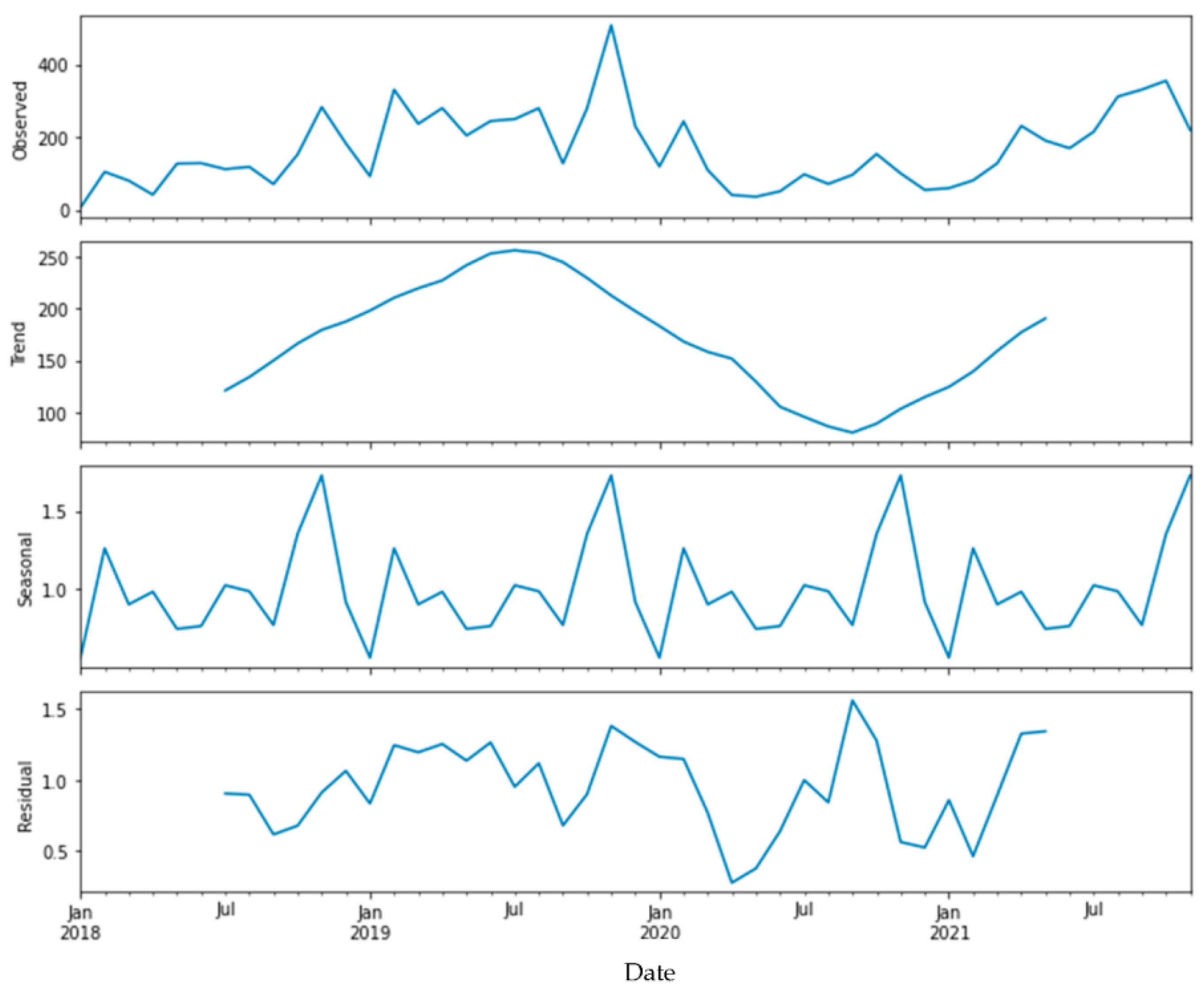
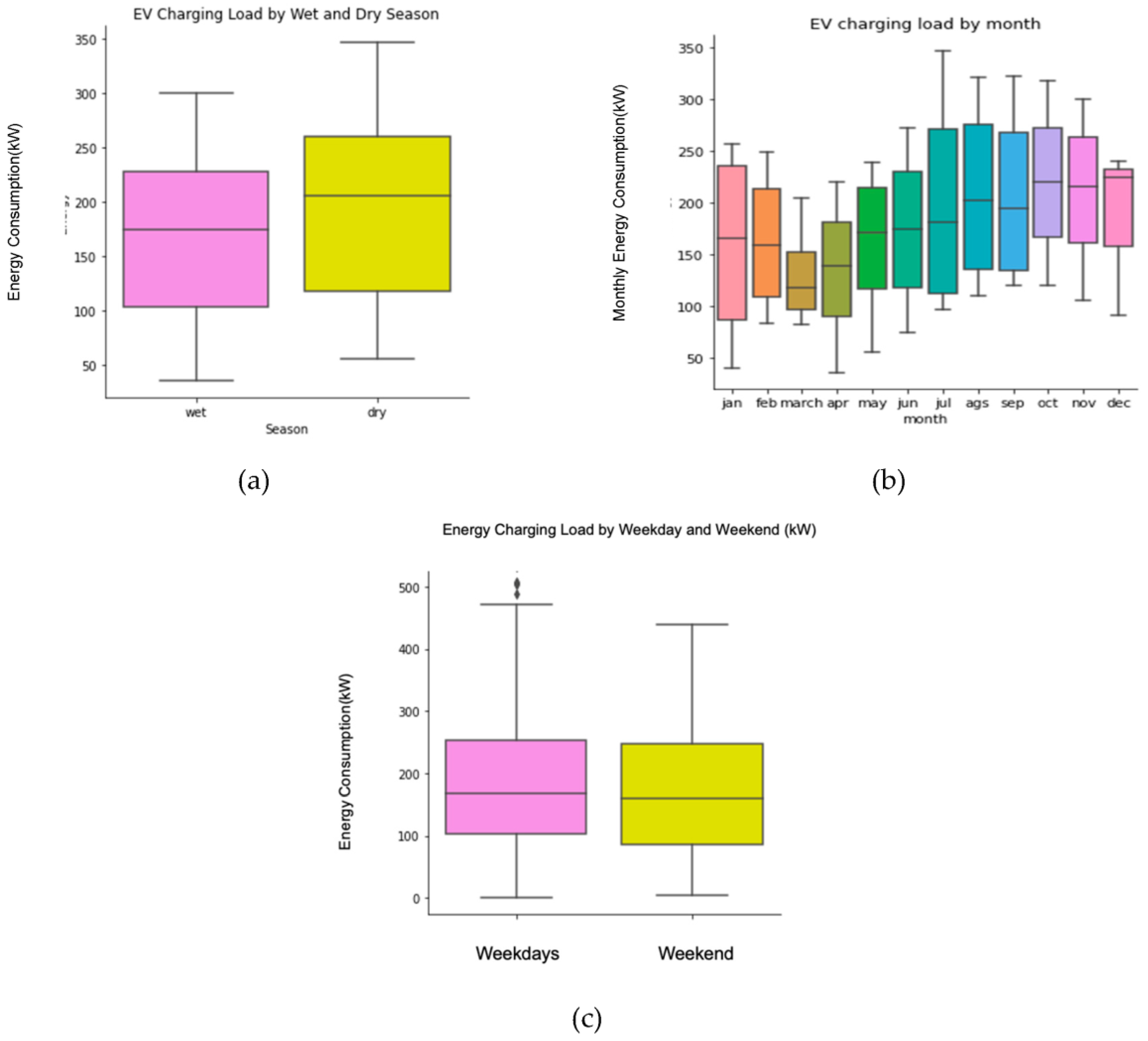
2.2. Data Analysis
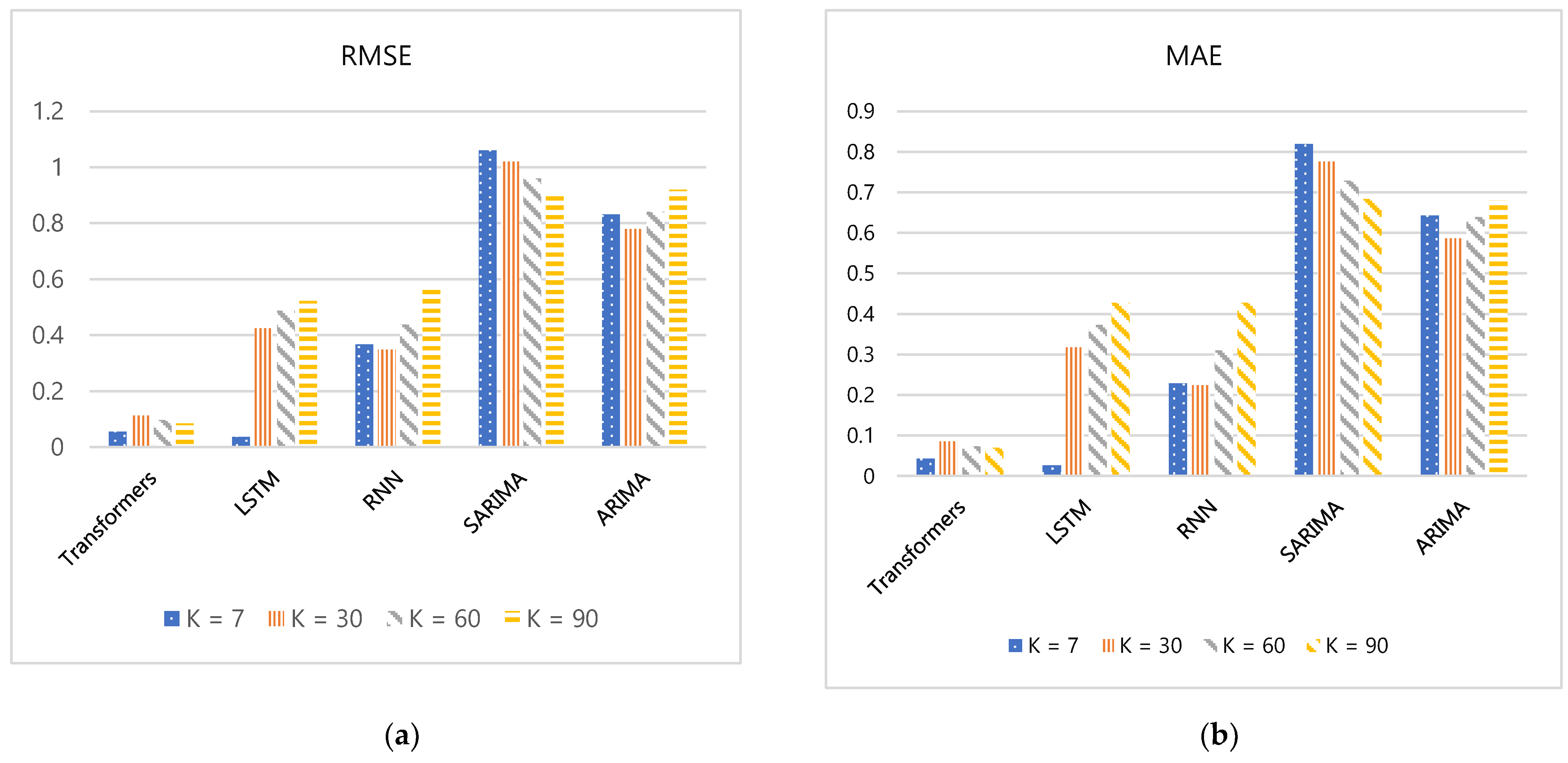
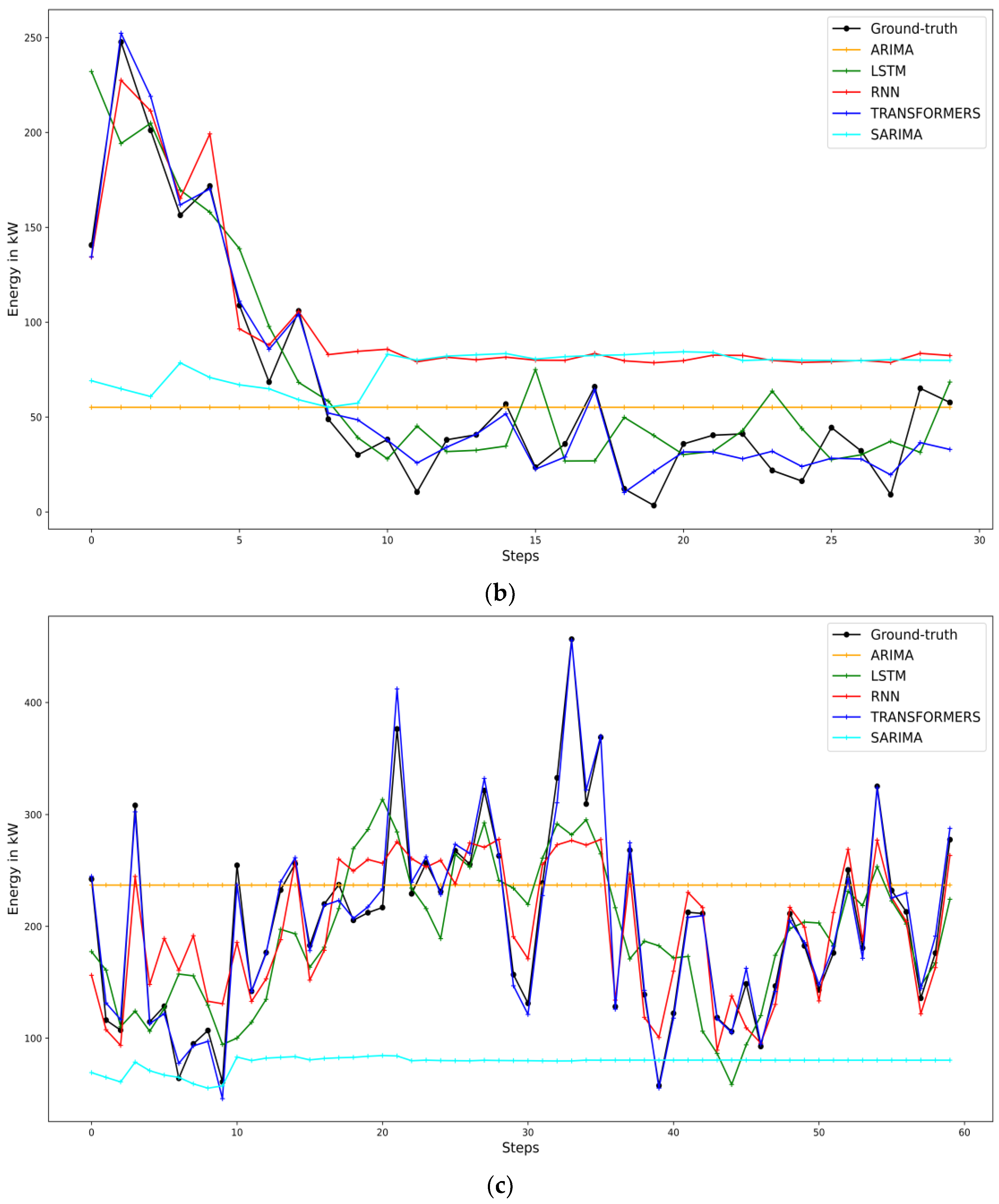
2.3. Performance Measurement
3. Results and Discussion
4. Conclusions
Author Contributions
Funding
Institutional Review Board Statement
Informed Consent Statement
Data Availability Statement
Conflicts of Interest
References
- Zheng, X.; Streimikiene, D.; Balezentis, T.; Mardani, A.; Cavallaro, F.; Liao, H. A review of greenhouse gas emission profiles, dynamics, and climate change mitigation efforts across the key climate change players. J. Clean. Prod. 2019, 234, 1113–1133. [Google Scholar] [CrossRef]
- Global EV Outlook 2021. 2021. Available online: https://www.iea.org/reports/global-ev-outlook-2021 (accessed on 22 January 2022).
- Yong, J.Y.; Ramachandaramurthy, V.K.; Tan, K.M.; Mithulananthan, N. A review on the state-of-the-art technologies of electric vehicle, its impacts and prospects. Renew. Sustain. Energy Rev. 2015, 49, 365–385. [Google Scholar] [CrossRef]
- Dubey, A.; Santoso, S. Electric vehicle charging on residential distribution systems: Impacts and mitigations. IEEE Access 2015, 3, 1871–1893. [Google Scholar] [CrossRef]
- Moon, H.; Park, S.Y.; Jeong, C.; Lee, J. Forecasting electricity demand of electric vehicles by analyzing consumers’ charging patterns. Transp. Res. Part D Transp. Environ. 2018, 62, 64–79. [Google Scholar] [CrossRef]
- Zhu, J.; Yang, Z.; Mourshed, M.; Guo, Y.; Zhou, Y.; Chang, Y.; Wei, Y.; Feng, S. Electric vehicle charging load forecasting: A comparative study of deep learning approaches. Energies 2019, 12, 2692. [Google Scholar] [CrossRef]
- Caliwag, A.C.; Lim, W. Hybrid VARMA and LSTM method for lithium-ion battery state-of-charge and output voltage forecasting in electric motorcycle applications. IEEE Access 2019, 7, 59680–59689. [Google Scholar] [CrossRef]
- Amini, M.H.; Kargarian, A.; Karabasoglu, O. ARIMA-based decoupled time series forecasting of electric vehicle charging demand for stochastic power system operation. Electr. Power Syst. Res. 2016, 140, 378–390. [Google Scholar] [CrossRef]
- Buzna, L.; De Falco, P.; Khormali, S.; Proto, D.; Straka, M. Electric vehicle load forecasting: A comparison between time series and machine learning approaches. In Proceedings of the 2019 1st International Conference on Energy Transition in the Mediterranean Area (SyNERGY MED), Cagliari, Italy, 28–30 May 2019. [Google Scholar]
- Louie, H.M. Time-series modeling of aggregated electric vehicle charging station load. Electr. Power Compon. Syst. 2017, 45, 1498–1511. [Google Scholar] [CrossRef]
- Khodayar, M.; Liu, G.; Wang, J.; Khodayar, M.E. Deep learning in power systems research: A review. CSEE J. Power Energy Syst. 2020, 7, 209–220. [Google Scholar]
- LeCun, Y.; Bengio, Y.; Hinton, G. Deep learning. Nature 2015, 521, 436–444. [Google Scholar] [CrossRef] [PubMed]
- Kumar, K.N.; Cheah, P.H.; Sivaneasan, B.; So, P.L.; Wang, D.Z. Electric vehicle charging profile prediction for efficient energy management in buildings. In Proceedings of the 2012 10th International Power & Energy Conference (IPEC), Ho Chi Minh City, VietNam, 12–13 December 2012. [Google Scholar]
- Jahangir, H.; Tayarani, H.; Ahmadian, A.; Golkar, M.A.; Miret, J.; Tayarani, M.; Gao, H.O. Charging demand of plug-in electric vehicles: Forecasting travel behavior based on a novel rough artificial neural network approach. J. Clean. Prod. 2019, 229, 10291044. [Google Scholar] [CrossRef]
- Hochreiter, S.; Schmidhuber, J. Long short-term memory. Neural Comput. 1997, 9, 1735–1780. [Google Scholar] [CrossRef] [PubMed]
- Chang, M.; Bae, S.; Cha, G.; Yoo, J. Aggregated electric vehicle fast-charging power demand analysis and forecast based on LSTM neural network. Sustainability 2021, 13, 13783. [Google Scholar] [CrossRef]
- Marino, D.L.; Amarasinghe, K.; Manic, M. Building energy load forecasting using deep neural networks. In Proceedings of the IECON 2016-42nd Annual Conference of the IEEE Industrial Electronics Society, Florence, Italy, 23–26 October 2016. [Google Scholar]
- Kong, W.; Dong, Z.Y.; Jia, Y.; Hill, D.J.; Xu, Y.; Zhang, Y. Short-term residential load forecasting based on LSTM recurrent neural network. IEEE Trans. Smart Grid 2017, 10, 841–851. [Google Scholar] [CrossRef]
- Kong, W.; Dong, Z.Y.; Jia, Y.; Hill, D.J.; Xu, Y.; Zhang, Y. Ultra-Short-Term Prediction of EV Aggregator’s Demond Response Flexibility Using ARIMA, Gaussian-ARIMA, LSTM and Gaussian-LSTM. In Proceedings of the 2021 3rd International Academic Exchange Conference on Science and Technology Innovation (IAECST), Guangzhou, China, 10–12 December 2021. [Google Scholar]
- Ahmed, S.; Nielsen, I.E.; Tripathi, A.; Siddiqui, S.; Rasool, G.; Ramachandran, R.P. Transformers in Time-series Analysis: A Tutorial. arXiv 2022, arXiv:2205.01138. [Google Scholar]
- Vaswani, A.; Shazeer, N.; Parmar, N.; Uszkoreit, J.; Jones, L.; Gomez, A.N.; Kaiser, Ł.; Polosukhin, I. Attention is all you need. arXiv 2017, arXiv:1706.03762. [Google Scholar]
- Devlin, J.; Chang, M.W.; Lee, K.; Toutanova, K. Bert: Pre-training of deep bidirectional transformers for language understanding. arXiv 2018, arXiv:1810.04805. [Google Scholar]
- Dong, L.; Xu, S.; Xu, B. Speech-transformer: A no-recurrence sequence-to-sequence model for speech recognition. In Proceedings of the 2018 IEEE International Conference on Acoustics, Speech and Signal Processing (ICASSP), Calgary, AB, Canada, 15–20 April 2018. [Google Scholar]
- Liu, Y.; Zhang, J.; Fang, L.; Jiang, Q.; Zhou, B. Multimodal motion prediction with stacked transformers. In Proceedings of the IEEE/CVF Conference on Computer Vision and Pattern Recognition, Nashville, TN, USA, 20–25 June 2021. [Google Scholar]
- Box, G.E.; Jenkins, G.M.; Reinsel, G.C.; Ljung, G.M. Time Series Analysis: Forecasting and Control; John Wiley & Sons: Hoboken, NJ, USA, 2015. [Google Scholar]
- Bahdanau, D.; Cho, K.; Bengio, Y. Neural machine translation by jointly learning to align and translate. arxiv 2014, arXiv:1409.0473. [Google Scholar]
- City of Boulder Open Data. 2021. Available online: https://open-data.bouldercolorado.gov/datasets/39288b03f8d54b39848a2df9f1c5fca2_0/explore (accessed on 28 December 2022).
- Paszke, A.; Gross, S.; Massa, F.; Lerer, A.; Bradbury, J.; Chanan, G.; Killeen, T.; Lin, Z.; Gimelshein, N.; Antiga, L.; et al. Pytorch: An imperative style, high-performance deep learning library. arXiv 2019, arXiv:1912.01703. [Google Scholar]


| EV Stations | Type | Number of Record | Energy Usage | |
|---|---|---|---|---|
| Min | Max | |||
| 25 | Disaggregated (EV charging Event) | 29,780 | 0.001 (kW/Event) | 85.2 (kW/Event) |
| Aggregated (Daily EV charging) | 1425 | 0.74 (kW/Day) | 531.6 (kW/Day) | |
| Variable | Feature | ARIMA | SARIMA | RNN | LSTM | Transformers |
|---|---|---|---|---|---|---|
| Load | EV charging load (kW/day) | + * | + | + | + | + |
| Calendar | Binary weekend (0 or 1) | + | + | + | ||
| Weather | Max temperature (°F) Min temperature (°F) Snow (mm/day) Precipitation (mm/day) | + | + | + |
| Hyper Parameters | Value |
|---|---|
| Hidden Dimension | 128 |
| Number of Epoch | 100 |
| Number of Layer | 1 |
| Number of Head | 8 |
| Steps Ahead (k) | Transformer | LSTM | RNN | SARIMA | ARIMA | |||||
|---|---|---|---|---|---|---|---|---|---|---|
| RMSE | MSE | RMSE | MSE | RMSE | MSE | RMSE | MSE | RMSE | MSE | |
| K = 7 | 0.055 | 0.043 | 0.036 | 0.026 | 0.367 | 0.229 | 1.06 | 0.819 | 0.831 | 0.643 |
| K = 30 | 0.112 | 0.085 | 0.425 | 0.317 | 0.348 | 0.224 | 1.02 | 0.776 | 0.779 | 0.586 |
| K = 60 | 0.096 | 0.073 | 0.488 | 0.373 | 0.438 | 0.310 | 0.960 | 0.729 | 0.841 | 0.639 |
| K = 90 | 0.085 | 0.070 | 0.522 | 0.427 | 0.564 | 0.427 | 0.903 | 0.683 | 0.920 | 0.680 |
Disclaimer/Publisher’s Note: The statements, opinions and data contained in all publications are solely those of the individual author(s) and contributor(s) and not of MDPI and/or the editor(s). MDPI and/or the editor(s) disclaim responsibility for any injury to people or property resulting from any ideas, methods, instructions or products referred to in the content. |
© 2023 by the authors. Licensee MDPI, Basel, Switzerland. This article is an open access article distributed under the terms and conditions of the Creative Commons Attribution (CC BY) license (https://creativecommons.org/licenses/by/4.0/).
Share and Cite
Koohfar, S.; Woldemariam, W.; Kumar, A. Prediction of Electric Vehicles Charging Demand: A Transformer-Based Deep Learning Approach. Sustainability 2023, 15, 2105. https://doi.org/10.3390/su15032105
Koohfar S, Woldemariam W, Kumar A. Prediction of Electric Vehicles Charging Demand: A Transformer-Based Deep Learning Approach. Sustainability. 2023; 15(3):2105. https://doi.org/10.3390/su15032105
Chicago/Turabian StyleKoohfar, Sahar, Wubeshet Woldemariam, and Amit Kumar. 2023. "Prediction of Electric Vehicles Charging Demand: A Transformer-Based Deep Learning Approach" Sustainability 15, no. 3: 2105. https://doi.org/10.3390/su15032105
APA StyleKoohfar, S., Woldemariam, W., & Kumar, A. (2023). Prediction of Electric Vehicles Charging Demand: A Transformer-Based Deep Learning Approach. Sustainability, 15(3), 2105. https://doi.org/10.3390/su15032105