Article

Development of Performance Measurement Models for Two-Lane Roads under Vehicular Platooning Using Conjugate Bayesian Analysis

1
Faculty of Civil Engineering, Shahrood University of Technology, Shahrood 36199-95161, Iran
2
Institute for Physical Infrastructure and Transportation (IPIT), University of Wisconsin–Milwaukee, Milwaukee, WI 53201, USA
3
Department of Engineering, Utah Valley University, Orem, UT 84058, USA
*
Author to whom correspondence should be addressed.
Sustainability 2023, 15(5), 4037; https://doi.org/10.3390/su15054037
Submission received: 29 December 2022 / Revised: 8 February 2023 / Accepted: 17 February 2023 / Published: 22 February 2023

Abstract

:
Vehicular platooning is one of the most challenging issues affecting the level of service (LOS) of two-lane roads. This phenomenon has been involved with variables governing performance measures. Thus, to improve the quality of these roads and predict a comprehensive model for future plans under this phenomenon, the present study aimed to evaluate the effect of vehicular platooning variables on performance measures and then identify the critical headways of vehicular platooning associated with the vehicle-gap-acceptance behavior. Multiple linear regression (MLR) and Bayesian linear regression (BLR) models were used to develop performance measurement models that are based on conjugate Bayesian analysis. The vehicular platooning was formed in the threshold of a time headway of 2.4 s. According to a comparative evaluation of the developed models, the best predictive model was found between the traffic flow and the number of followers per capacity (NFPC). In addition, the BLR model showed a higher accuracy rate in predicting NFPC compared with the MLR model due to low errors and high prediction performance. Thus, NFPC was introduced as a surrogate performance measure, which had a premier capability to predict the LOS for unsaturated and saturated traffic conditions compared with the two performance measures from the Highway Capacity Manual (2010), including percent time spent following and average travel speed.

1. Introduction

Two-way two-lane rural roads play important roles in road transportation facilities. They serve two primary purposes of transportation and accessibility thanks to their uninterrupted traffic-flow facilities and no limitation on the movement of vehicles along the roads. According to the Iranian Road Maintenance and Transportation Organization [1], two-way two-lane rural roads account for approximately 30% of the network roads in Iran. Owing to the complex interaction of vehicles in one direction and the opposite direction, measuring traffic performance on two-lane roads is a challenging issue for traffic engineers and managers. Further, because two-lane roads are the essential roads in rural districts, platooning formation from the high percentage of heavy vehicles, the higher likelihood of overtaking and lane changes is widespread in comparison with other urban roads [2,3,4,5]. On urban roads, owing to the high speed and the high number of lanes, the formation of vehicular platooning is relatively lower than that on rural roads, such as two-lane roads [6]. Given the complexity of this phenomenon, traffic engineers frequently look for methods and measures to define the traffic capacity and quality of traffic flows for two-lane roads. According to some studies [7,8,9,10,11], vehicular platooning significantly affects the quality of the operational performance of two-lane roads, including the average travel speed (ATS) and capacity, leading to a reduction in the level of service (LOS). When platoons form in two-lane roads, variables that contribute to performance measures affect the quality of traffic flow and, accordingly, decrease operational performance [3,12,13,14,15,16]. Consequently, reducing the quality of the traffic flow and operational performance under the effect of vehicular platooning has a negative impact on the safety and risk of drivers, playing a role in collisions [17,18,19,20,21]. The Highway Capacity Manual (HCM) [22] has defined two performance measures for determining the LOS for two-lane roads, including percent time spent following (PTSF) and ATS. Platooning is defined when the time headway between follower and leader vehicles is 3 s [22,23]. However, other studies have shown that PTSF under various traffic-flow conditions is inconsistent with the 3 s rule [23,24,25]. Al-Kaisy and Durbin [2] introduced the ATS measure as the average percentage of travel time for the platoon of vehicles at a speed rate below the average. Owing to limitations in performance measures (PTSF and ATS), several studies have been conducted, and they have resulted in the introduction of some additional performance measures, including follower density (FD), the ATS of passenger cars (ATSpc), the percentage of vehicles impeded (PI), and other measures [2,25,26,27,28].
Thus, introducing a surrogate measure as an alternative could help traffic engineers to better measure traffic performance and the rate of the traffic stream. Further, the improvement of models for the performance measures leads to an accurate estimation of the performance and thereby the LOS of two-lane roads. In addition, strategies and plans based on the development of two-lane roads according to necessity would be competitive and allow the implementation of road management organizations and road traffic controllers. In this regard, the present study investigates the effect of vehicular platooning characteristics on performance measures for two-lane roads, followed by identifying the critical headways of platooning by accounting for the vehicle-gap-acceptance behavior. Four case studies on two-lane roads in the Gilan province of Iran were used in this study. This province has attractive sightseeing areas. Most of the roads leading to these areas are accessed by two-lane roads. Additionally, the industrial areas in the province are accessed by two-lane roads. These case studies were selected on the basis of the high demands of their traffic, their heavy traffic flow, and thereby their more-frequent vehicular platooning.
Next, the Pearson correlation is applied to examine the relationships between vehicular platooning and performance measures. Depending on the normal conjugate function, a Bayesian approach or multiple linear regression (MLR) models are proposed for the BLR model in order to develop performance measures for two-lane roads as a function of vehicular platooning. Further, a comparative evaluation of Bayesian linear regression (BLR) and MLR models is considered on the basis of prediction performance criteria and statistical criteria, including the p-value, F-value, and R2 value, for finding the most-influential vehicular platooning variable on performance measures. Thereafter, the LOS is evaluated among the measures for identifying the optimal performance measure. Finally, in accordance with the optimal measure, the classification results of two-lane roads are compared with the HCM [22].
The remaining sections of this study are explained as follows. Section 2 reviews the studies relevant to the examination of the platooning phenomenon and its effect on traffic performance by using platooning variables and performance measures from two-lane roads. Thereafter, it discusses the research gap in the previous studies to highlight the paper’s overarching idea and its applied methods. Section 3 describes the research methodology for two-lane roads and denotes the platooning variables and performance measures by using the empirical data from different sites in Iran. Further, the Pearson correlation is evaluated as the initial investigation of the relationship between variables and measures in this section. Thereafter, the MLR and BLR models are applied to develop performance measurement models and select a surrogate measure as the optimal performance measure under the effect of vehicular platooning. Accordingly, a comparison evaluation is provided throughout the proposed models. Section 4 presents the results and a discussion of the proposed measures and developed models. Finally, Section 5 concludes the research findings.

2. Literature Review

Numerous studies related to the evaluation of the effect of vehicular platooning on the quality of traffic flow and traffic measures in two-lane roads are described, as follows. Kim and Elefteriadou [29] investigated the effect of heavy vehicles (%HV) on the performance measures of two-lane roads using ATS and capacity. The results indicated that capacity decreased by 40% when ATS was reduced. Penmetsa et al. [30] proposed a measure for the LOS classification by using the number of followers as a proportion of capacity (NFPC). The results revealed the superiority of this measure over the PTSF measure in the HCM [22] to evaluate the quality of traffic flow and traffic performance on Indian roads. Jrew et al. [31] used performance measures such as ATS, free-flow speed (FFS), and the PTSF to evaluate the LOS of two-lane roads in Jordan. They found that an increase in ATS and FFS led to an improvement in the LOS.
Some studies have also investigated the effect of vehicle type, ATS, FFS, and PTSF on the LOS of two-lane roads. The results revealed that capacity improved as ATS and FFS increased, while PTSF was accompanied by a decrease in capacity and the LOS [32,33]. Bessa and Setti [34] introduced PTSF and ATS as the main performance measures of two-lane roads affecting the LOS of two-lane roads. Moreover, Gaur and Mirchandani [35] proposed vehicular platooning in two-lane roads by using traffic flow, follower density (FD), number of platoons, and time headway distribution for measuring traffic performance. Arasan and Kashani [36] also identified platoon size as the most effective vehicular platooning variable on two-lane-road performance measures, including ATS and percentage of followers (PF). Some studies have emphasized the role of vehicle-gap acceptance, along with the traffic flow of two-lane roads, on platoon size by using time headway as a threshold value for identifying vehicular platooning [37,38,39,40,41]. Moreover, some other studies have indicated that platooning depends on time headway. Time headway for platooning ranges from 3 to 7 s, significantly affecting performance measures such as ATS, FD, and platoon speed [2,42,43]. Yang et al. [44] found that %HV and platoon size were negatively related to traffic flow on Dutch highways.
Some studies have also reported that under the emergence of time headways and %HV, vehicular platooning negatively affected the performance measures of two-lane roads, including ATS and FFS [45,46,47]. Other studies have proposed that platoon size and %HV are the main vehicular platooning variables influencing the performance measures of two-lane roads, measures such as ATS, FFS, FD, and PF [6,48]. Hashim and Abdel-Wahed [49] introduced FD as the surrogate performance measure among ATS, FFS, %HV, ATS of passenger cars (ATSpc), ATSPC as a percentage of the free-flow speed of passenger cars (ATSpc/FFSpc), and ATS as a percentage of free-flow speed (ATS/FFS) under vehicular platooning for evaluating the LOS of two-lane roads in Egypt. They indicated that traffic flow has the greatest effect on FD. Moreover, some studies have investigated the effect of vehicular platooning variables (i.e., traffic flow and time headway) on ATS in two-lane rural roads. They showed that time headway was strongly correlated with ATS rather than with traffic flow [50,51]. Likewise, Moreno [52] introduced %HV as the variable most common to cause platooning compared with other variables (i.e., traffic flow, time headway, and opposing flow), impacting traffic performance variables such as the ATS and FD of two-lane roads in Spain. Al-Zerjawi et al. [53] found a strong relationship between some platooning variables, such as flow, time headway, the number of overtaking (NO) vehicles, and performance measures such as the ATS and PF of two-lane roads in Al-Mishkhab, Iraq. Furthermore, Ahmed and Easa [54] developed performance measurement models that were based on the PTSF of two-lane roads by means of the threshold of time headway. Kim [55] observed that the %HV is the most-influential vehicular platooning variable compared with platoon size and NO on performance measures such as ATS, FD, and PTSF. Previous studies have demonstrated that the most effective vehicular platooning variables on the performance measures include the %HV and platoon size; other performance measures include ATS, FD, and platoon speed [33,56,57,58,59,60,61].
Jin et al. [62], in a study focused on evaluating the impact of vehicle platooning on highway congestion, used a fluid-queuing approach. They showed that as the number of platoons increases, it leads to more congestion in traffic flow. Mena-Oreja et al. [63] also investigated the platooning maneuvers on traffic flow under mixed traffic conditions. They concluded that mixed traffic flow has an influencing effect on increasing the number of platoons. Kita and Yamada [64] introduced a vehicle velocity control approach that accounted for platoon merging. They showed that their model could successfully control the speed of drivers with a combination of platooning and merging. Zhu et al. [10] developed a dynamic model that was based on the formation of vehicular platooning on two-lane roads. Their results showed that an increase in the percentage of heavy vehicles led to more platooning in traffic flow. Moreover, Zhu et al. [10] concluded that a heterogeneous traffic flow, compared with a homogenous traffic flow, has a direct effect on the emergence of platoons. Al-Kaisy [4] reported that two-lane roads have more potential for vehicular platooning compared with other roads owing to the traffic composition of vehicles, overtaking maneuvers, and the speed beneficence of cars in comparison with heavy vehicles. Mauro et al. [65] developed a statistical model to evaluate the platoons of vehicles on two-lane roads. They indicated that the platoons of vehicles play important roles in traffic-flow characteristics. Further, developed statistical models provide a better performance prediction of the quality of two-lane roads than conventional statistical models do.
Therefore, a review of the previous studies relevant to the effect of vehicular platooning on the performance measures of two-lane roads, as shown in Table 1, revealed that no recent study has comprehensively evaluated the effect of vehicular platooning characteristics on the quality of traffic flow and traffic performance (i.e., time headway, platoon size, %HV, and opposing flow) and performance measures (i.e., ATS, platoon speed, NO, FD, PI, PF, NFPC, ATSpc, ATSpc/FFSpc, and ATS/FFS). The present study evaluated vehicular platooning under the critical thresholds of time headway by using vehicle-gap-acceptance behavior and the relationships between platooning variables influencing performance measures. Thereafter, the MLR and BLR models, based on regression and conjugate Bayesian analysis, respectively, were taken into consideration to develop performance measurement models. Accordingly, the optimal surrogate measures were selected on the basis of statistical criteria. Finally, the surrogate measure was compared with the HCM [22] regarding the effect of vehicular platooning on the LOS of two-lane roads.

3. Research Method

In the present study, first, vehicular platooning was evaluated by using vehicle-gap-acceptance behavior to determine the threshold of time headway for measuring platooning variables. Thereafter, the effects of vehicular platooning variables on the quality of traffic performance on two-lane roads were investigated. In this step, the platooning variables were extracted from the video recordings. Straight and longitudinal traps of 30 m were selected, one per site at four sites in Iran. The weather conditions were daylight, clear, and sunny, and the pavement had a suitable condition. In addition, during the videography, we controlled the effects of longitudinal slope, intersections, and horizontal alignments in the straight sections of the road. After collecting empirical data, the videography analysis method was performed to extract field data at 30 frames per second by using videography software.
Second, the relationships between platooning variables and performance measures were examined using the Pearson correlation to determine the initial relationships between these variables. After examining the relationships, the MLR and BLR models, based on the regression approach and the conjugate Bayesian analysis, respectively, were provided for the development of performance measures for the variables and measures in order to determine the most-influential variables on measures according to statistical criteria such as R2 value, p-value, significant F-value, and errors. Thereafter, a surrogate measure associated with the most effective variables was introduced by using the developed models and by comparing it with the HCM [22]. Thus, in the present study, the following performance measures were investigated:
  • ATS: this measure is the best-known performance measure for evaluating road users’ perceptions of the quality of traffic flow on two-lane roads [22].
  • ATSPC: this measure is more important than ATS on two-lane roads because passenger cars have a greater variety of ATSs than heavy vehicles do under different traffic conditions [6,66].
  • ATS/FFS: this measure shows the average speed reduction from interactions with other vehicles. Reducing this measure is accompanied by a decrease in the LOS. Because the FFS of roads changes under various traffic conditions, including FFS in the ATS could control the reduction rate of the LOS in two-lane roads [6].
  • ATSPC/FFSPC: this measure is defined similarly to ATS/FFS, but it refers only to passenger cars because of the sensitive interaction of their speeds under various traffic conditions compared with heavy vehicles, especially under high traffic flow [26].
  • PF: this measure denotes the percentage of vehicles with short headways in the traffic flow. This measure is obtained on the basis of the headway, in which the HCM considers 3 s [22] as the time headway for estimating PF. However, for other roads, the time headway should be modified.
  • FD: this measure represents the number of followers in a directional traffic flow over a given unit of length, which is defined as 1 km or 1 mile. It is important to consider the degree of congestion through PF and the density of two-lane roads [22,25]. This measure is obtained by using density (D) and PF according to Equations (1) and (2), as follows:
D = Q A T S .
F D = D × P F .
where Q is traffic flow (veh/h), A T S is the average travel speed (km/h), F D is the follower density (veh/km), D is the density (veh/km), and P F is the percentage of followers (%).
  • Percent impeded (PI): this measure represents the percentage of vehicles impeded in the vehicular platoon’s traffic flow [2,67]. PI is calculated by using Equation (3), as follows:
P I = P P × P i .
where P P is the probability of a vehicle in the vehicular platoon based on the time headway considered for platoon and P i is the probability that a vehicle will be impeded in the platoon.
  • NO: this measure is the most popular measure for evaluating the LOS of two-lane roads under platooning, reflecting the freedom of maneuverability [7,68,69].
  • Platoon speed: one of the characteristics of vehicular platooning in a two-lane road under the formation of the platoon of vehicles is platoon speed in the direction of traffic flow, based on the following vehicle headway and slow-moving vehicles [70]. Vehicles in the platoon have a speed less than the ATS of the traffic flow [2].
  • NFPC: this measure is introduced as a criterion for evaluating the effect of vehicular platooning and potential followers in platoon size and the degree of congestion as NFPC [30]. Thus, Equation (4) is proposed as a function of NF and capacity in two-lane roads, as follows:
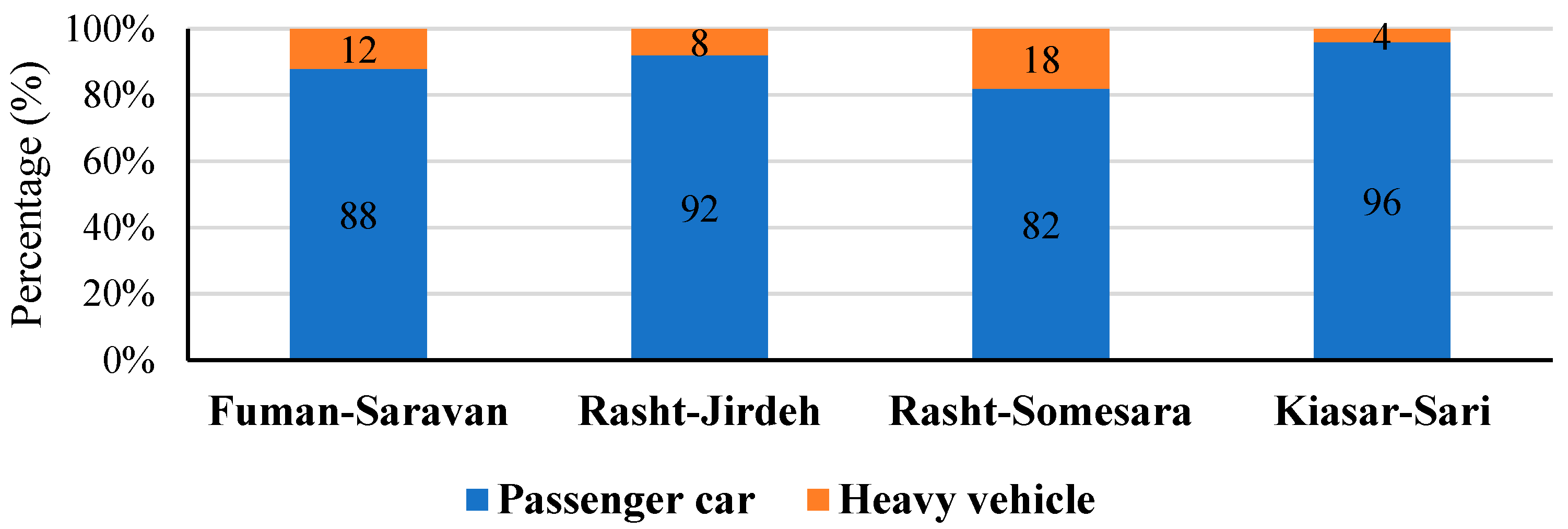
N F P C = N F max ( f ( Q ) ) .
where N F P C is a number of followers per capacity in two-lane roads, N F is the number of followers (veh/h), and max ( f ( Q ) ) is the maximum traffic flow (veh/h).

3.1. Case Study

In the present study, vehicular platooning variables and performance measures were examined as the empirical data from four sites of two-lane roads in the Gilan and Mazandaran provinces of Iran, including Rasht-Somesara, Fuman-Saravan, Rasht-Jirdeh, and Kiasar-Sari roads. During the collection of the field data, traffic flow varied, and the traffic included mainly drivers with light or heavy vehicles. In addition, the speed limit was 90 km/h, and the width of each road lane was 3.65 m. Figure 1 represents the composition of the traffic flow by the vehicle type passing on the two-lane roads. As shown in Figure 1, Kiasar-Sari’s maximum percentage of passenger cars is about 96%, and the minimum percentage of heavy vehicles is approximately 4%. However, Rasht-Somesara’s maximum percentage of heavy vehicles was about 18%, and the minimum percentage of passenger cars was nearly 82%.

3.2. Data Collection

In the present study, the empirical data were collected from four sites of two-lane roads using 5 min intervals over a total of 8 h. Thus, the sample size was considered as 96 for all roads. For modeling purposes and to obtain a comprehensive model that is based on the proposed model, a summary of all data sets after the initial analysis is shown in Table 2. All data sets consist of statistical information, including minimum, maximum, mean, standard deviation, and variance for platooning variables such as flow, opposing flow, time headway, %HV, and platoon size. Further, Table 2 represents the statistical information for describing performance measures such as ATS, ATSpc, ATSpc/FFSpc, ATS/FFS, NO, PF, FD, PI, platoon speed, and NFPC. The coefficient-of-variation (CV) values are highest for platoon size, flow, and opposing flow, indicating higher dispersion. This implies that these performance measures such as FD, NO, and NFPC are more sensitive to variables with higher CV. Thus, it is essential to investigate the effect of vehicular platooning on performance and the relationships between the variables and measures.
Figure 2 indicates the results from the examination of time headway after including gap-acceptance behavior and platoon speed. Figure 2a illustrates a 1 s interval of time headway for estimating the critical value as the threshold of vehicular platooning according to the vehicle-gap-acceptance behavior and the intersection of the accepted and rejected gaps from the selected four sites of two-lane roads. According to Figure 2a, the accepted and rejected gaps intersect in a time headway of 2.4 s. Further, Figure 2b demonstrates the relationship between the average platoon speed and the time headway of drivers regarding the formation of vehicular platooning on the studied roads. According to Figure 2b, it can be inferred that as the platoon speed of vehicles increases, this leads to a reduction in time headway, and the gap acceptance of drivers reaches the critical point. Further, as shown in Figure 2b, most of the platoons formed have a time headway longer than 2.4 s. In time headways shorter than 2.4 s, platoon size based on the field data decreases. Thus, an increase in the platoon speed causes a reduction in time headway, and the number of platoons decreases. Further, as seen in Figure 2b, the platoon size of vehicles has its maximum value as a platoon speed between 20 to 40 km/h.

3.3. MLR Model

Linear regression models are one of the most widely used methods in statistical analysis, and researchers have applied these methods in various applied sciences and engineering fields. Different linear regression models are recommended depending on the number of independent and dependent variables [71]. The MLR model is an appropriate statistical tool to test whether there is an influence from independent variables on a dependent variable and predict the value of the dependent variable, where the dependent variable y consists of n observations and k independent variables ( x 1 , x 2 , , x j ) [72]. Before applying the MLR model, the Pearson correlation is used to determine whether there is statistical evidence for a relationship between the independent and dependent variables [73]. Consider the following regression model with various explanatory variables and coefficients by using Equations (5) and (6), as follows [74]:
Y = β 0 + β 1 X 1 + β 2 X 2 + + β j X i j + ε i .
Y = X β + ε .
Thus, the MLR model in the form of a matrix is written as follows:
Y = [ y 1 y 1 y n ] ;   X = [ 1 x 11 x 1 j 1 x 21 x 2 j 1 x n 1 x n j ] ;   β = [ β 0 β 1 β j ] ;   ε = [ ε 1 ε 2 ε n ] .
where Y is the vector of observed random variables, which is a random normal vector by dimension n ; X is the independent observation matrix, which consists of n × ( k + 1 ) dimension and is named the design matrix; β is the vector of dimension ( j + 1 ) of the coefficient in the regression; and ε is the random error vector of dimension n of the ith observation for i = 1, 2,…, n.
In Equation (7), β could be obtained by using Equation (8), based on the ordinary least square (OLS) method, which is as expressed:
β ^ = ( X X ) 1 X Y .
where X is the transpose of matrix X .

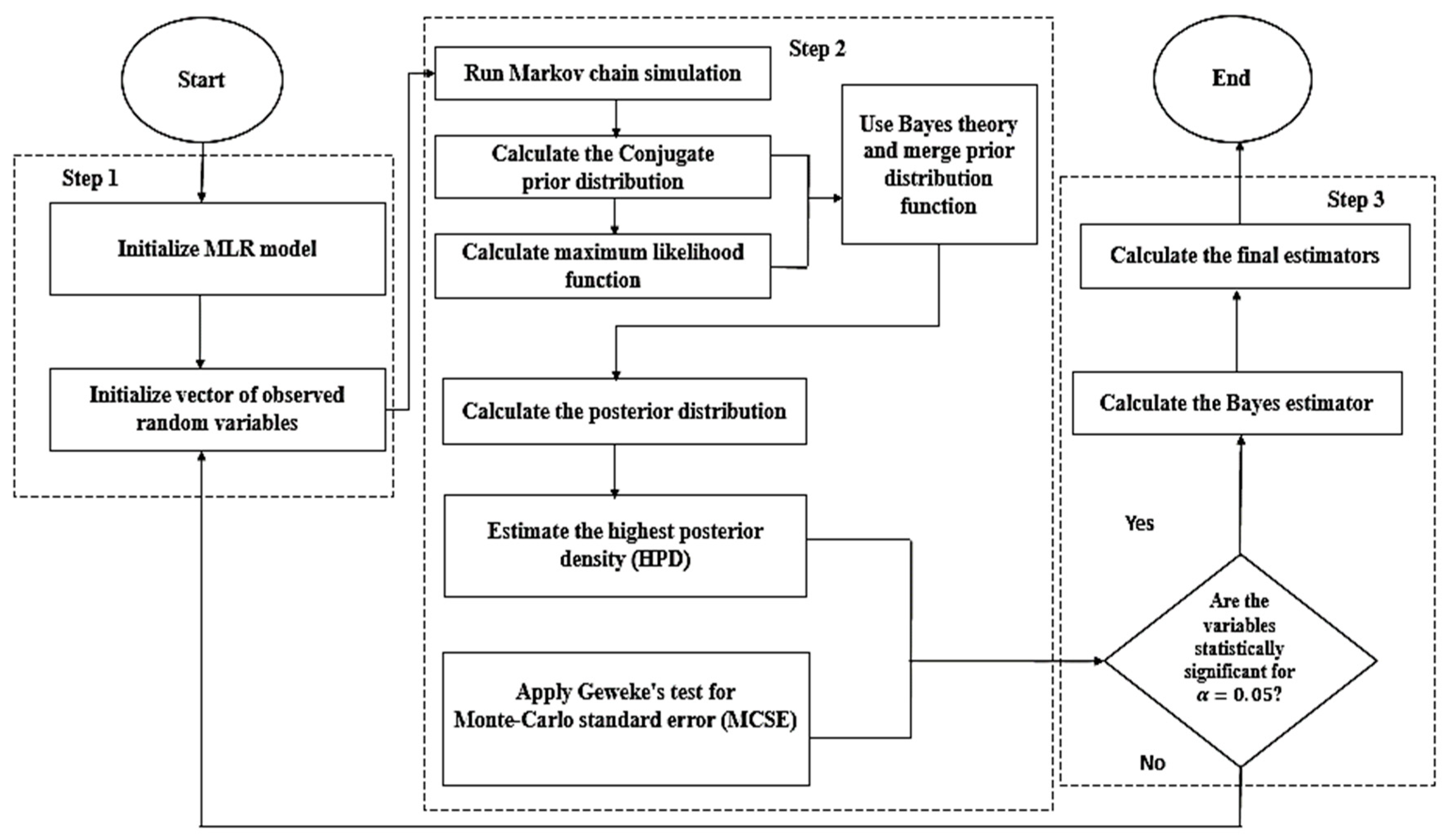
3.4. BLR Model Using Conjugate Prior Distribution

Recently, conjugate Bayesian analysis has been used as a predictive model of output values in statistics and other engineering sciences [73]. This model, thanks to its utilizing Bayesian theory, is better able to sufficiently predict output data compared with other statistical models, such as multiple regression models [75,76,77]. Other advantages of using conjugate Bayesian analysis compared with statistical models include having lower errors and more-reliable accuracy [78]. Thus, the BLR model is one of the most common regression techniques because the Bayesian approach uses the parameter estimation method. The Bayesian approach is based on the prior function, likelihood distribution function, and posterior distribution function. This approach is a new method among statistical methods, playing a modifier role in the improvement of MLR models because the BLR model is formulated on the basis of the MLR model [79,80,81,82]. The main difference between the classical methods and the Bayesian approach is that the parameter β is an unknown parameter. In classical methods, β is estimated via the probability distribution f ( x , β ) , while in the Bayesian approach, β is considered as a random variable with probability distribution g 2 ( β ) as the function of the likelihood function L ( x , β ) and prior distribution g 1 ( β ) . Thus, in the Bayesian approach, the posterior distribution g 2 ( β ) is obtained by multiplying the prior distribution by the likelihood function, leading to accurate parameter estimation β [83,84,85]. In this approach, the parameter β is taken into account with random variables, including β 1 ,   β 2 ,   ,   β n and the probability function. The probability function indicates all the information on and experiences from the parameters. Thereafter, the prior information is added to the observed sample information. Because this approach is unbiased, more samples lead to further average values of the samples and thus accurate estimation of parameter β [86,87]. The steps involved in the BLR model are summarized in Figure A1 in Appendix A. Consider the following regression model given in Equation (9):
Y = X   β + ε
where Y is the vector of observed random variables, which is a random normal vector by dimension n ; X is the independent observation matrix, which consists of n × ( k + 1 ) dimension and is named the design matrix; β is the vector of dimension ( j + 1 ) of the coefficient in the regression; and ε is the random error vector of dimension n . Thus, the BLR model, based on the dependent variable and error ε , is written as follows:
Y n ( X β , σ 2 I n ) and   ε n ( 0 , σ 2 I n )
where σ 2 is the variance and I n is the identity matrix. Therefore, the maximum likelihood function, based on the sample information and normal distribution, is represented in Equation (11), as follows:
L ( β , σ | y , x ) = 1 ( 2 π ) n 2 σ n exp { 1 2 σ 2 [ ( Y X β ) ( Y X β ) ] }
For simplicity, Equation (11), in terms of its dependent and independent variables, and Equations (12) and (13) are expressed as follows:
( Y X β ) ( Y X β ) = Y Y Y X β X β Y + β X X β .
( Y X β ) ( Y X β ) = Y Y 2 X β Y + β X X β .
which assume that b 0 = Z 1 X X Y and Z = X X .
Thereafter, by substituting the sum of the squared estimate of errors ( S S E ) into Equations (12) and (13), Equation (14) is obtained, as follows:
( Y X β ) ( Y X β ) = [ S S E ( b 0 ) + ( β b 0 ) Z ( β b 0 ) ] .
Thus, the maximum likelihood function of Equation (11) is rewritten in Equation (15), as follows:
L ( β , σ | y , x ) = 1 ( 2 π ) n 2 σ n exp { 1 2 σ 2 [ S S E ( b 0 ) + ( β b 0 ) Z ( β b 0 ) ] } .
By deleting the constants and the S S E ( b 0 ) , which has the parameters β and the information σ 2 , Equation (16) is expressed, as follows:
L ( β ) exp { 1 2 σ 2 [ ( β b 0 ) Z ( β b 0 ) ] } .
The normal distribution of the parameter β is called the prior distribution, as g 1 ( β ) , which is estimated by Equation (17), as follows:
g 1 ( β ) exp { 1 2 σ 2 [ ( β β 0 ) Ω 1 ( β β 0 ) ] } .
where Ω is the precision matrix X that is estimated by Ω = X X S 2 , where X and S 2 are the transpose of matrix X and an estimator of σ 2 , respectively. Thus, the posterior distribution g 2 ( β | y ) is obtained by using Bayes’s theory and merging the prior distribution function with the maximum likelihood function L ( β ) according to Equation (16) and the prior distribution g 1 ( β ) by using Equation (17), as denoted by g 2 ( β | y ) g 1 ( β ) . L ( β ) in Equation (18).
g 2 ( β | y ) exp { 1 2 σ 2 [ ( β b 0 ) Z ( b β 0 ) + ( β β 0 ) Ω 1 ( β β 0 ) ] } .
Equation (18) is simplified by using assumptions such as c * = ( b 0 β 0 ) Z Ω * Ω 1 ( b 0 + β 0 ) , b * = Ω * ( Z b 0 + Ω 1 β 0 ) , and Ω * = ( Z + Ω 1 ) 1 . Hence, the posterior distribution is reformulated according to Equation (18) and written in Equation (19), as follows:
g 2 ( β | y ) exp { 1 2 σ 2 [ ( β b * ) Ω * 1 ( β b * ) + c * ] } .
Equation (19) indicates the posterior distribution as a normal distribution of a mean b * , a variance σ 2 , and covariance matrix σ 2 Ω * , where β is N ( b * , σ 2 Ω * ) . In Equations (17) and (19), the prior and posterior distributions have a normal distribution. Therefore, the prior distribution is named the conjugate prior distribution, which verifies the prior probability distribution. Accordingly, the posterior distribution is applied to estimate the regression model parameters. The following Bayes estimators are related to the parameters of the regression model β from Equations (20)–(22), which are given as follows:
Ω * = ( Z + Ω 1 ) 1 ,   b b a y e s * = Ω * ( Z b 0 + Ω 1 β 0 ) .
b b a y e s * = ( Z + Ω 1 ) 1 Z b 0 + ( Z + Ω 1 ) 1 Ω 1 β 0 .
Thus, simplifying Equation (21) to calculate the estimated regression model leads to the formation of Equation (22), which is written as follows:
b b a y e s * = ( H 1 b 0 ) + ( H 2 β 0 ) .
where H 1 = ( Z + Ω 1 ) 1 Z and H 2 = ( Z + Ω 1 ) 1 Ω 1 . In Equation (22), the regression parameters are obtained to calculate the maximum likelihood weighted by the weights matrix and the prior distribution average [86].

3.5. Comparison of Prediction Performance of Models

The prediction performance for the MLR and BLR models, using performance measures under vehicular platooning, is compared with the mean absolute percentage error (MAPE). The purpose is to select the best predictive model in terms of acceptable error and accuracy by using Equation (23), which is expressed as follows [30,80]:
M A P E = 1 N i = 1 n | y i y ^ i y i | × 100 % .
where y i is the observed dependent variable based on the field data and y ^ i denotes the predicted value for the developed models based on the performance measures.

4. Results and Discussion

After examining the platooning variables and performance measures from the empirical data, the initial investigation of the relationships between these two variables using the Pearson correlation is represented. Thereafter, the results of the development of the MLR and BLR models for predicting performance measures concerning platooning variables are obtained. Regarding the developed MLR and BLR models, the relationships between dependent and independent variables are examined using statistical criteria such as the R2, F-value, p-value, and t-value, along with errors in prediction performance, to select the most-influential platooning variable on the performance measures. Thus, according to the best fit model with low error and high prediction accuracy, a surrogate measure is proposed as a performance measure to evaluate the LOS in two-lane roads. The results obtained from the comparison evaluation in the present study with the HCM [22] are shown. The obtained results and findings are described in the following section.

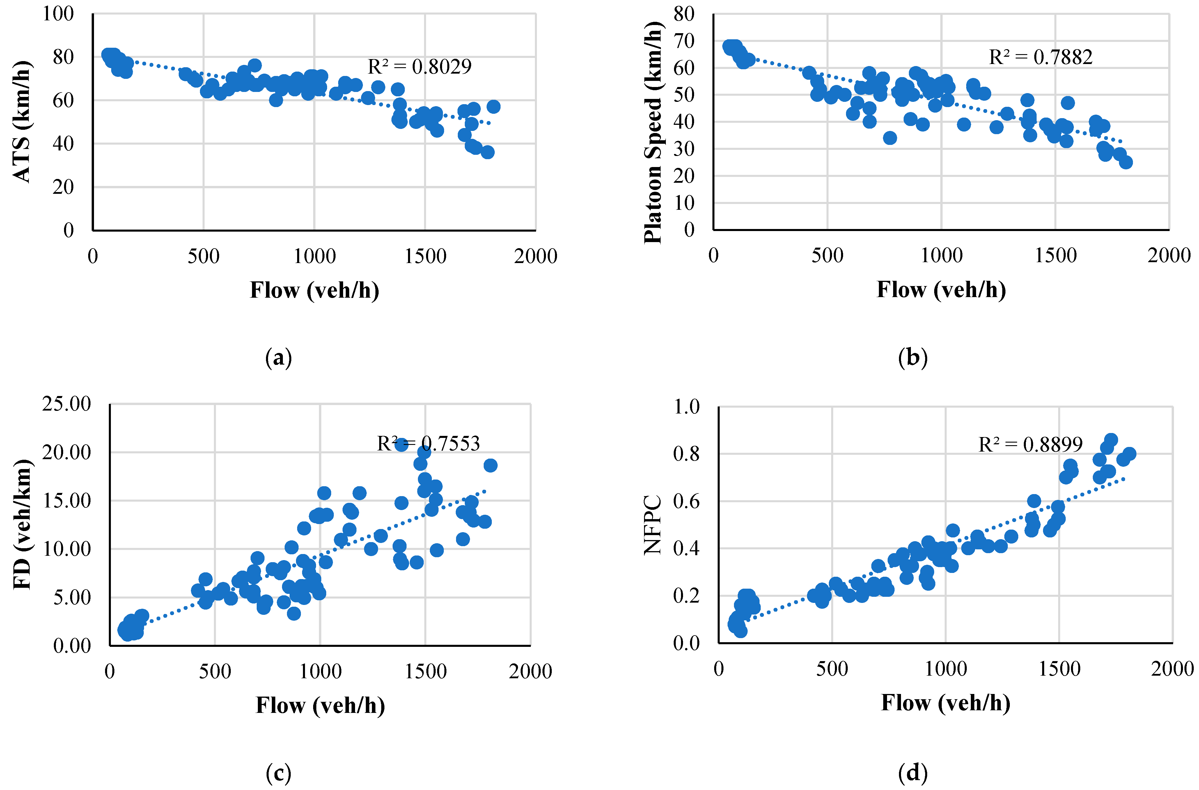
4.1. Pearson Correlation and MLR Model
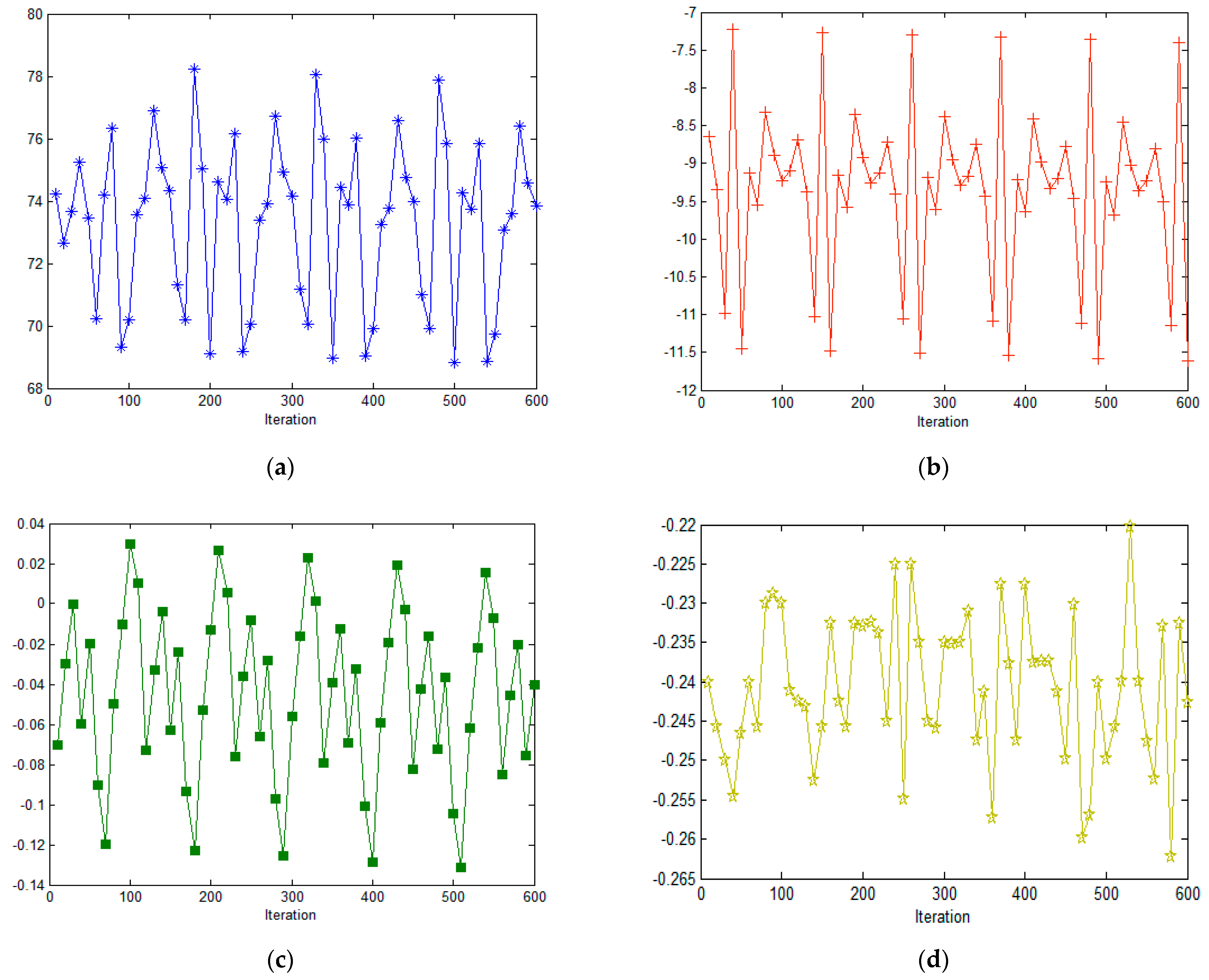
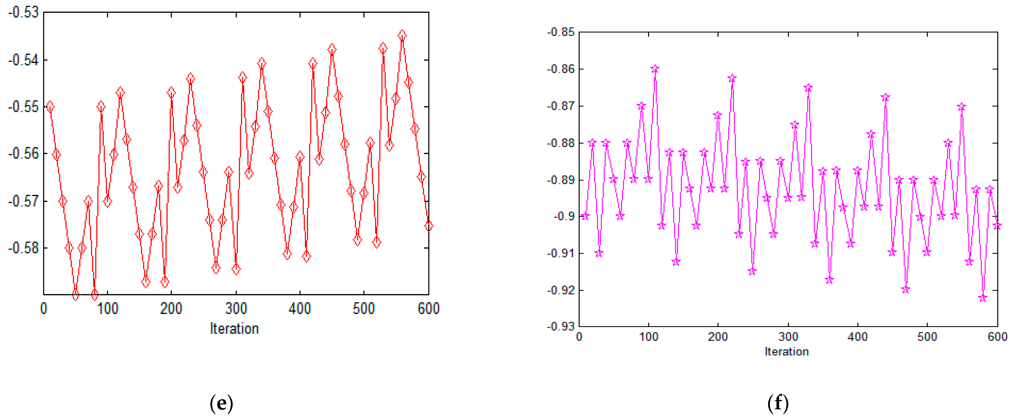
After examining the platooning variables and performance measures in Table 2, a Pearson correlation was performed, and the results are displayed in Table 3. According to Table 3, it can be inferred that traffic flow has the highest correlation with NFPC, ATS, platoon speed, FD, PI, PF, NO, and ATSPC, in that order. Opposing flow has a strong correlation with NFPC, PF, ATS, FD, and PI, in that order. Further, examining the relationships between %HV and performance measures revealed that %HV has a high correlation with FD, ATS, PF, and PI, in that order. In addition, platoon size is significantly related to platoon speed, PI, ATS, and ATSpc, in that order. Time headway also has a significant correlation with ATS, NFPC, ATSpc, and FD, in that order.
After applying Equations (5)–(8) for the MLR model, the results were obtained, and they are shown in Table 4. According to Table 4 and statistical criteria such as the R2, F-value, p-value, and absolute value of the t-value, traffic flow significantly influences the performance measures, including NFPC, ATS, platoon speed, FD, PI, PF, NO, and ATSPC. Moreover, among the performance measures in Table 4, flow is identified as the most-influential variable on NFPC thanks to its higher absolute value of coefficient, t-value, p-value (less than 0.05), and R2 for the best predictive model. However, other platooning variables indicate a weak correlation with the performance measures in MLR models.

4.2. BLR Model

The platooning variables were applied to predict performance measures in two-lane roads. The results were obtained for each performance measure as a function of platooning variables in the BLR model by using Equations (9)–(22). The present study obtained the prior and posterior distributions by using the Markov chain Monte Carlo (MCMC) method for 600 iterations. Further, the noninformative independent normal prior distributions with variance and the Gamma inverse distribution have been used for regression coefficients and parameter σ 2 , respectively (Table 5). The highest posterior density (HPD) intervals for all parameters have been determined at a significance level of 0.05 in all models. Owing to the constraint of space, only the characteristics of prior and posterior distributions were provided in Table 5 and Table 6, as well as in Figure 3, which was used to estimate the parameters of vehicular platooning affecting ATS on the basis of the trace plot of the MCMC chains. A similar scheme is followed for estimating parameters in other performance measures, the results of which are presented in Table 7. Thus, as it can be observed, the results based on the Monte Carlo standard error (MCSE), Geweke’s test, and the p-value suggest that the generated chains did not converge for all parameters of the investigated model at any significant level. The results in Table 7 indicate that the relationship between platooning variables and NFPC is stronger than the relationship between other platooning variables and performance measures regarding the higher R2 value and the p-value among the proposed BLR models. Further, flow significantly affects the performance measures, compared with other variables, thanks to a higher coefficient and a p-value of less than 0.05.
The following general vector of parameter β for prior distribution is estimated according to the noninformative independent normal prior distributions of each platooning variable concerning ATS, which are obtained in Equation (24), as follows:
β 0 = ( 75.34 10.99 0.09 0.23 0.61 1.23 ) .
The precision matrix Ω is followed by Equation (25):
Ω = exp ( + 5 ) ( 0.0013 0.0378 0.0532 0.0771 0.0037 0.0643 0.0102 0.8512 1.3220 2.1080 0.6800 0.0489 0.0678 1.9710 6.5081 7.5501 0.6170 2.0130 0.0410 0.8830 7.2810 8.4600 0.5981 2.617 0.0026 0.0594 0.4406 0.6901 0.0047 0.0855 0.0112 0.3950 1.5980 2.5124 0.0051 0.8059 ) .
Thus, Z , which is estimated according to Equation (26), is written as follows:
Z = exp ( + 5 ) ( 0.0020 0.0214 0.0841 0.0971 0.0043 0.0351 0.0235 0.9816 1.6319 2.3210 0.8760 0.0767 0.0863 1.4535 7.7646 8.6541 0.7640 2.1580 0.0753 0.6741 8.6531 9.6280 0.6530 2.7657 0.0033 0.0673 0.5421 0.8076 0.0053 0.0951 0.0233 0.4216 2.2670 2.7678 0.0071 0.8719 ) .
To obtain the BLR model on the basis of using Equation (22), H 1 and H 2 are applied as the weights matrix for the independent matrix and the prior distribution, respectively, which are calculated by Equations (27) and (28), as follows:
H 1 = ( Z + Ω 1 ) 1 Z = ( 0.0014 0.0015 0.0046 0.0075 0.0049 0.0128 0.0037 0.0018 0.0023 0.0014 0.0078 0.0269 0.0064 0.0038 0.0047 0.0043 0.0642 0.0050 0.0057 0.0045 0.0033 0.0082 0.0534 0.0087 0.0038 0.0077 0.0026 0.0079 0.0155 0.0954 0.0036 0.0019 0.0072 0.8100 0.0137 0.2739 ) .
H 2 = ( Z + Ω 1 ) 1 Ω 1 = ( 0.0011 0.0012 0.0043 0.0070 0.0043 0.0012 0.0035 0.0016 0.0019 0.0010 0.0760 0.0025 0.0060 0.0031 0.0042 0.0040 0.0610 0.0480 0.0046 0.0041 0.0029 0.0074 0.0481 0.0076 0.0033 0.0067 0.0019 0.0066 0.0143 0.0851 0.0030 0.0016 0.0065 0.7478 0.0127 0.2019 ) .
Thus, the parameters are estimated and denoted by b 0 for the platooning variables, as expressed in Equation (29):
b 0 = ( + 59.85 5.76 0.12 0.40 0.15 0.37 ) .
Thereafter, by applying Equation (22), the Bayes estimator for the parameters of the BLR model is obtained from Equation (30):
b * b a y e s = ( 73.64 9.76 0.04 0.25 0.55 0.87 ) .
Therefore, the final BLR model is obtained by Equation (31), and shown in Table 7, as follows:
Y ^ b a y e s = 73.64 9.76 X 1 0.04 X 2 0.25 X 3 0.55 X 4 0.87 X 5 .

4.3. Analysis of the Most-Influential Platooning Variable on Performance Measures

For an analysis of the effect of platooning variables and performance measures in MLR and BLR models, see Table 4 and Table 7 and Figure 4, which depict the results of the highest relationships. As displayed in Figure 4, traffic flow has a strong relationship with NFPC, ATS, platoon speed, and FD, in that order. This means that an increase in traffic flow leads to a decrease in ATS and platoon speed and an increase in NFPC and FD. Further, according to the results of Figure 4, the most-influential platooning variable on performance measure regarding R2 coefficient is the relationship between flow and NFPC, compared with other variables, as verified by the results in Table 4 and Table 7. Thus, the best predictive model for representing the surrogate performance measure is the relationship between flow and NFPC in the MLR and BLR models.
Further, for the validation of and a comparative evaluation of the proposed models regarding the best fit for platooning variables and performance measures, the results of the predicted performance measures are examined via empirical data, and each measure’s error (MAPE) under platooning variables is presented in Figure 5. As shown in Figure 5, the BLR model has worse error prediction performance compared with the MLR model. Further, the lowest error is related to NFPC in each model, suggesting that selecting this measure is an optimal choice as a surrogate performance measure among the performance measures, compared with other measures. Moreover, regarding the relationship between flow and NFPC in both models, the results of the best fit models and errors are obtained for MAPE according to Equation (23) (Table 8 and Figure 6). According to Table 8, the BLR model is the best predictive model for evaluating NFPC under traffic flow. Further, it can be inferred that the BLR model can predict NFPC as the most-influential performance measure to classify the LOS of two-lane roads by using statistical analysis and overall error values (Figure 6). Therefore, using BLR, based on the conjugate Bayesian analysis, is proposed as a predictive tool for determining the effect of platooning variables on performance measures thanks to its fewer errors and high prediction performance compared with the MLR model. The results indicate that conjugate Bayesian analysis offers better prediction performance in comparison with the MLP model. These results are the same as the results of other studies, which showed that the BLR model is better than MLR in other engineering fields [30,76,77].

4.4. Evaluation of the LOS by Using the Preferred Performance Measure

To evaluate the LOS in two-lane roads, the surrogate measure is selected as the preferred performance measure for the proposed models and the average values. As displayed in Figure 4, Figure 5 and Figure 6, the proposed surrogate performance measure is selected as NFPC thanks to its higher statistical criteria compared with those of other performance measures. Thus, the results of the proposed classification for the LOS are selected according to the BLR model (Table 9). This measure can classify LOS A and LOS B as between 0.20 and 0.40, respectively. Further, according to this measure, LOS C to LOS D ranges from 0.40 to 0.80. However, the HCM [22] determines the ATS to be greater than 88 km/h and PTSF to be less than 35% for LOS A. Moreover, LOS C to LOS E is classified by using an ATS between 64 and 80 km/h and a PTSF between 50% and 80%.
Likewise, Table 10 illustrates the comparison between capacity and the LOS with the HCM [22] for the selected four sites of the two-lane roads on the basis of the NFPC. As demonstrated in Table 10, the HCM [22] classifies the LOS for the studied roads from C to E by using the ATS and PTSF, respectively, while in the present study, the LOS is classified from B to D according to NFPC measure. Thus, according to the surrogate measure in the present study, the LOS for the Rasht-Jirdeh and Kiasar-Sari roads is classified as B. However, regarding the HCM [22], the LOS for the Rasht-Jirdeh, Kiasar-Sari, and Fuman-Saravan roads is classified as C and D. Further, for the Fuman-Saravan and Rasht-Somesara roads with high traffic flow, the LOS is classified as C and D, respectively, on the basis of the NFPC. Accordingly, the proposed surrogate measure can effectively predict the LOS for the unsaturated and saturated conditions in two-lane roads when compared to the HCM [22]. Therefore, it can be concluded that for class I roads, the NFPC could act as a surrogate performance measure to better predict the LOS of two-lane roads under unsaturated and saturated conditions compared to using the two measures of the HCM [22], namely PTSF and ATS.

4.5. Policy Implications

The results of the present study show that vehicular platooning is an important phenomenon on two-lane roads. This traffic phenomenon involves traffic-flow characteristics on these roads. Regarding the importance of these roads for rural areas, evaluating traffic-flow characteristics and developing performance measures on two-lane roads will help road and transportation organizations to improve the capacity of these roads under high traffic demands in the future. Thus, to facilitate and increase the satisfaction of users on two-lane roads, the first step is to accurately evaluate traffic-flow characteristics on the basis of the developed performance measures.
The quality of two-lane roads should be examined on the basis of the obtained NFPC in the present study rather than ATS and PTSF because the NFPC could efficiently be related to the capacity of drivers and the number of vehicles following others. However, other studies have focused on the assessment of the quality of two-lane roads by using ATS and PTSF, and these studies did not mention the relation to the capacity of roads [22,48,89]. Because the complexity of the LOS of two-lane roads at near free-flow speed and under congested traffic-flow conditions increases, the measurement of the LOS under these conditions might not provide an accurate LOS to traffic engineers, given that the obtained results on performance measures such as ATS and PTSF in the present study showed that these measures do not provide exact predictions.
Furthermore, to stabilize the traffic flow on two-lane roads, it is necessary to connect the formation of platoons to capacity, as obtained from these variables in the present study, thanks to the developed performance measure models. These models, owing to their including the formation of platoons of vehicles and their effects on traffic-flow characteristics, are reliable and inform optimal policy recommendations for future traffic environments involving two-lane roads. Further, the criterion for the formation of platooning vehicles regarding time headway and the gap acceptance of drivers helps to count the number of followers in the queues on two-lane roads. Thus, to obtain the optimal policy regarding the driver satisfaction on two-lane roads under traffic conditions, the present study recommends the formation of platooning vehicles at intervals higher than 2.4 s, which decreases as the speed of drivers increases. Additionally, NFPC, compared with ATS and PTSF, could sufficiently work under various traffic conditions.
Moreover, new models must account for BLR, compared with conventional models such as MLR, to offer better performance at predicting the LOS for two-lane roads. Therefore, regarding the present threshold of forming platooning vehicles (2.4 s), the proposed performance measures (NFPC), and the BLR model, policymakers could enhance the traffic environment for drivers on two-lane roads.

5. Conclusions

Two-lane rural roads play important roles in urban transportation and accessibility. Vehicular platooning has been a challenging issue for engineers aiming to propose an optimal performance measure for evaluating the traffic performance in two-lane roads. Therefore, the present study aimed first to assess the effect of vehicular platooning variables on performance measures at four selected two-lane roads in Iran. The vehicular platooning variables included traffic flow, time headway, platoon size, %HV, and opposing flow. Performance measures included ATS, FD, PI, PF, NFPC, ATSpc, ATSpc/FFSpc, ATS/FFS, NO, and platoon speed. Further, this study identified the critical headways for the formation of vehicular platooning on the basis of vehicle-gap-acceptance behavior. The MLR and BLR models were applied to develop performance measurement models and find the best fit model for the surrogate measure and statistical criteria. The obtained results are described as follows:
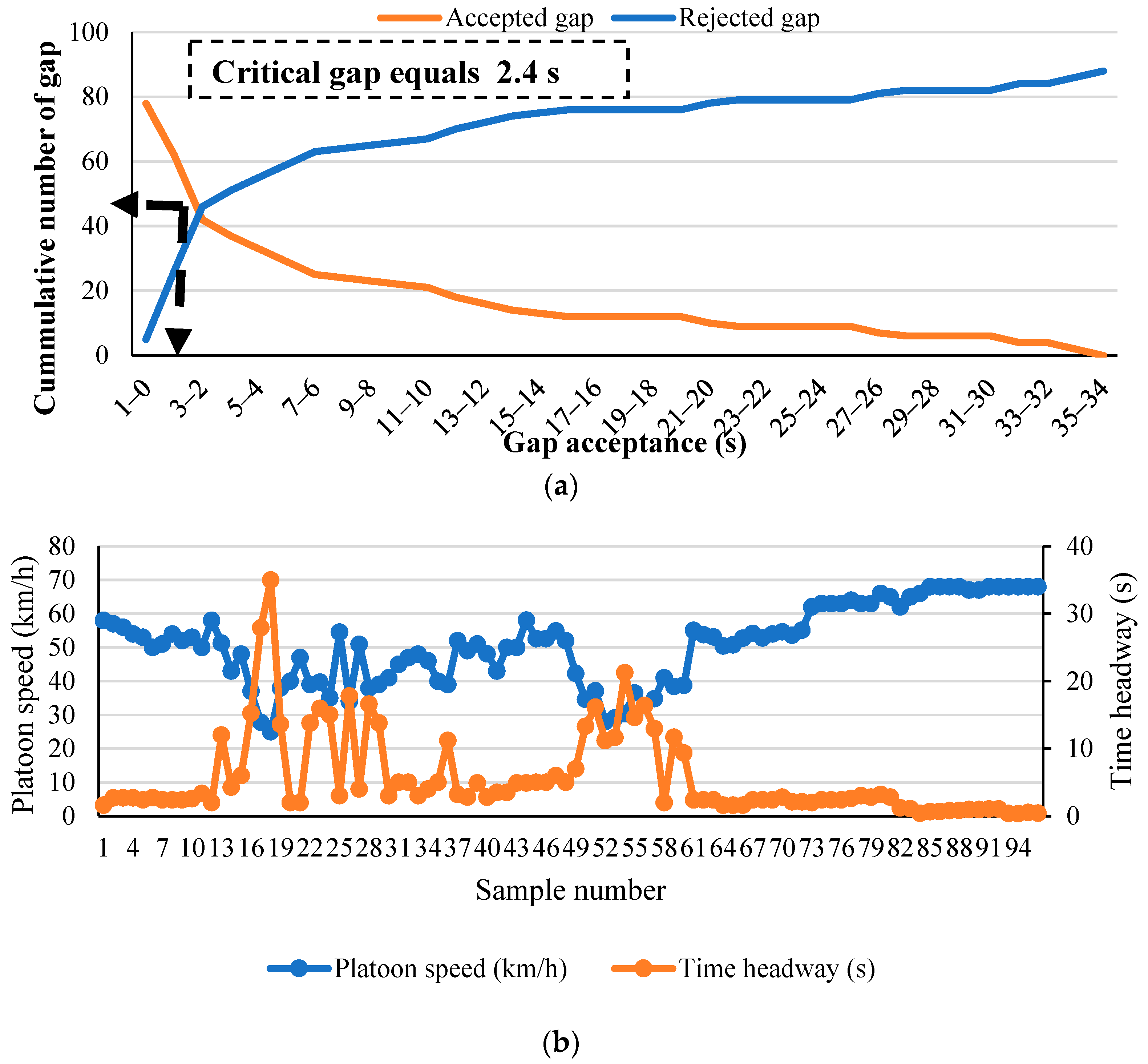
  • According to the vehicle-gap-acceptance behavior, it was found that headways less than 2.4 s were identified as the thresholds for forming platooning in two-lane roads.
  • The results of the Pearson correlation indicated that the traffic flow has the highest correlation with NFPC, ATS, platoon speed, FD, PI, PF, NO, and ATSPC, in that order. Moreover, the opposing flow strongly correlated with NFPC, PF, ATS, FD, and PI, in that order. Further, by examining the relationship between the %HV and performance measures, it can be concluded that the %HV had a high correlation with FD, ATS, PF, and PI, in that order. The relationships between platoon size and platoon speed, PI, ATS, and ATSpc are significant, in that order. Time headway was also significantly correlated with ATS, NFPC, ATSpc, and FD, in that order.
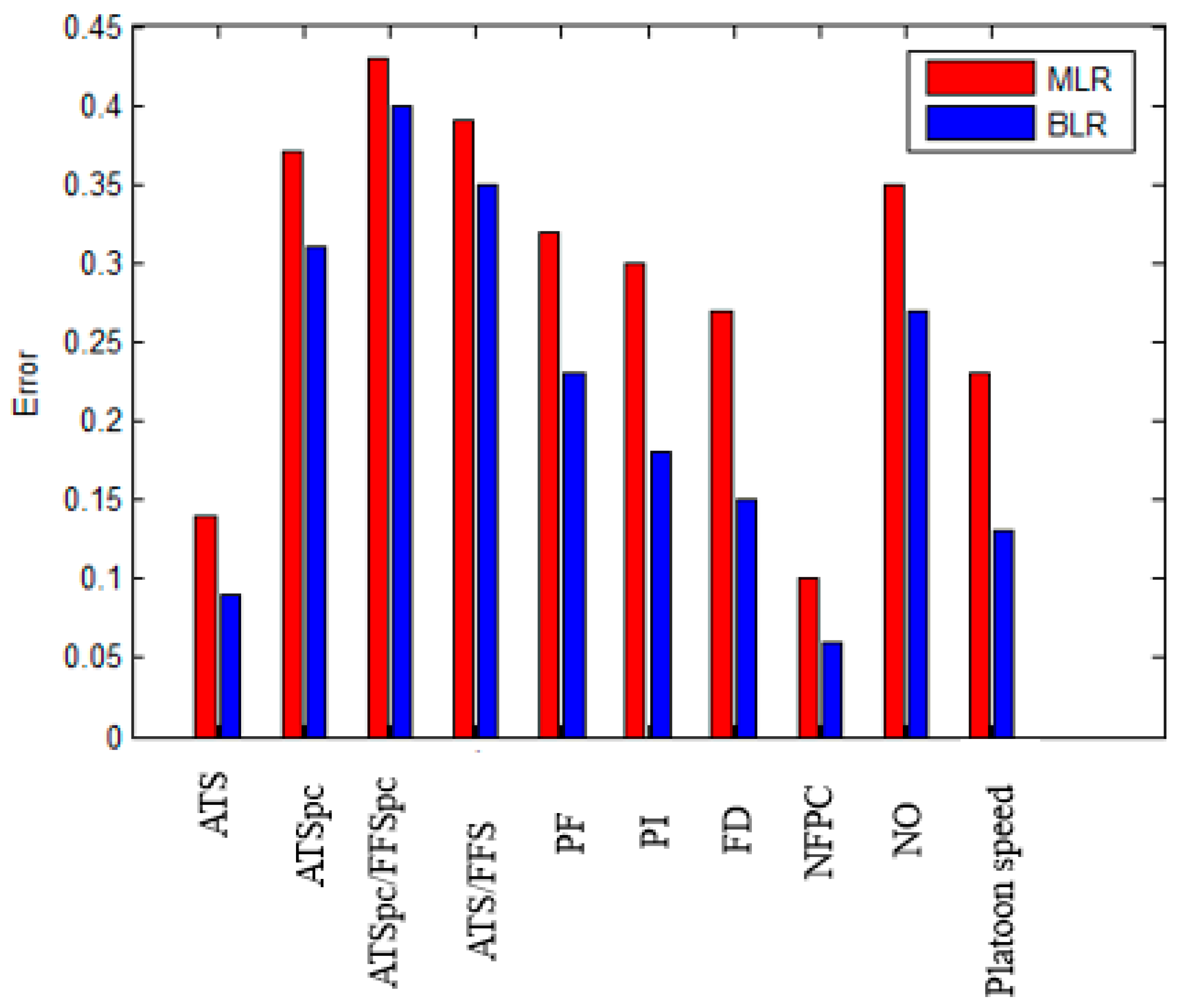
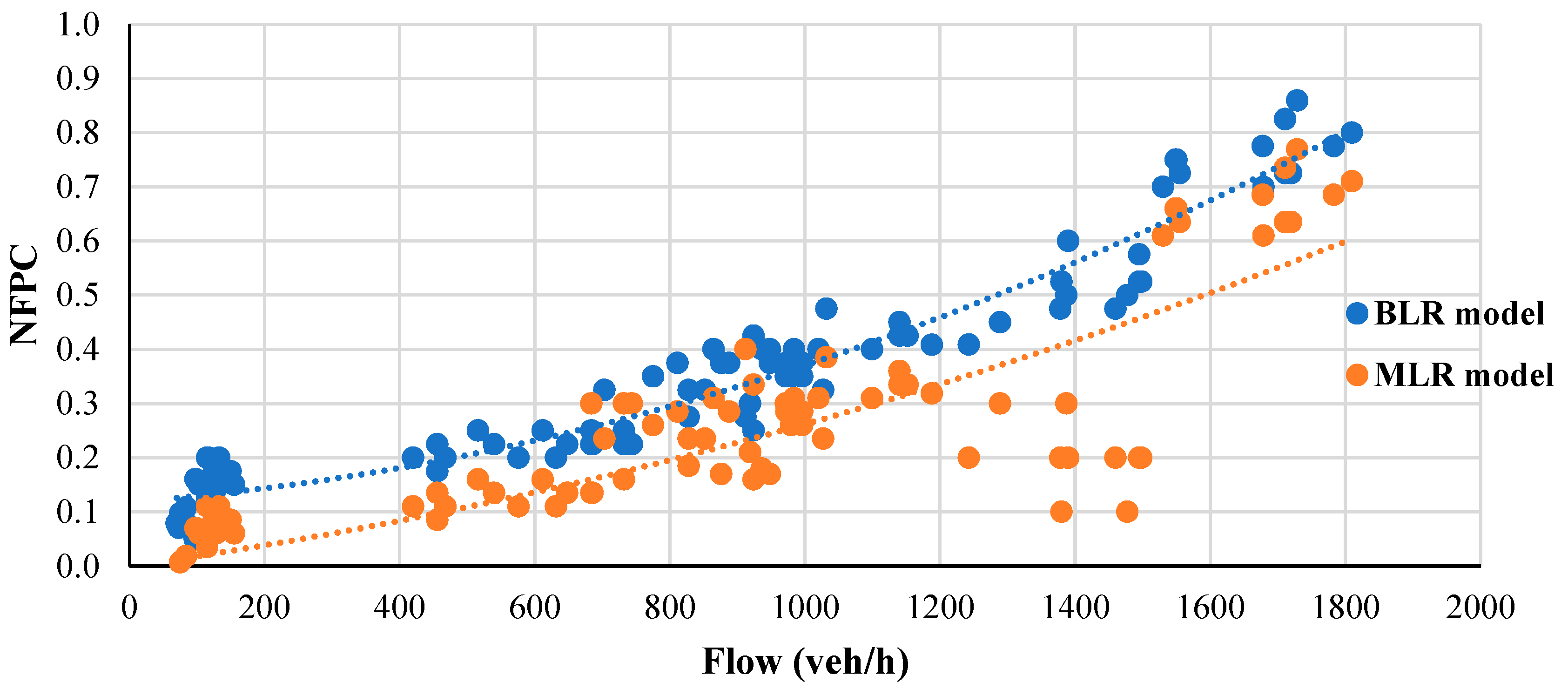
  • The results of the developed MLR and BLR models indicated that BLR could predict NFPC as the most-influential performance measure to classify the LOS of two-lane roads on the basis of accuracy and error values.
  • The comparison evaluation from the proposed surrogate measures with performance measures recommended in the HCM [22] indicated that the NFPC could be a surrogate performance measure for better predicting the LOS under unsaturated and saturated conditions compared to the two measures of the HCM [22], namely PTSF and ATS, under vehicular platooning.
The results of the present study could be useful for traffic engineers and road organizations aiming to estimate the quality of two-lane roads on the basis of the proposed performance measure. Further, the criterion for the formation of vehicular platooning regarding time headway and the gap acceptance of drivers on two-lane roads could help traffic engineers to accurately investigate the beginning of the formation of platooning for calculating queues and platoon size. Another application of the present study is the development of new models for evaluating the quality of two-lane roads in terms of the LOS and vehicular platooning and comparing them with conventional models, such as regression models. Other macroscopic performance models can be developed on the basis of the proposed surrogate performance measure in the present study to calibrate the models according to the traffic conditions of other sites. From a road safety aspect, this research could improve the quality of two-lane roads for the improvement of the driver’s gap-acceptance behavior, which is involved in the proposed surrogate performance measure of two-lane roads for preventing the occurrence of collisions that are due to the formation of platoons and due to overtaking maneuvers.

Author Contributions

Conceptualization, H.S., I.A., K.S. and F.H.; methodology, H.S., I.A. and F.H.; software, F.H. and I.A.; validation, H.S., I.A., K.S. and F.H.; formal analysis, H.S., I.A. and F.H.; investigation, H.S., I.A. and F.H.; resources, H.S., I.A. and F.H.; data curation, H.S., I.A. and F.H.; writing—original draft preparation, H.S., I.A., K.S. and F.H.; writing—review and editing, H.S., I.A., K.S. and F.H.; visualization, I.A. and F.H.; supervision, I.A.; project administration, I.A. All authors have read and agreed to the published version of the manuscript.

Funding

The authors received no financial support for this research paper.

Institutional Review Board Statement

Not applicable.

Informed Consent Statement

Not applicable.

Data Availability Statement

The data are available upon request to the corresponding author.

Conflicts of Interest

The authors declare no conflict of interest in the present study.

Appendix A

Figure A1. Flowchart of the BLR model. Notes: BLR: Bayesian linear regression; MLR: multiple linear regression.
Sustainability 15 04037 g0a1

References

  1. Iran Road Maintenance and Transportation Organization, RMTO [Online] Iran Road Maintenance and Transportation Organization. 2009. Available online: http://www.rmto.ir/newtto/Download/Roads.pdf (accessed on 15 January 2009).
  2. Al-Kaisy, A.; Durbin, C. Platooning on two-lane two-way highways: An empirical investigation. J. Adv. Transp. 2009, 43, 71–88. [Google Scholar] [CrossRef]
  3. Moreno, A.; Llorca, C.; Washburn, S.; Bessa, J.; Hale, D.; Garcia, A. Modification of the highway capacity manual’s two-lane highway analysis procedure for spanish conditions. J. Adv. Transp. 2016, 50, 1650–1665. [Google Scholar] [CrossRef]
  4. Al-Kaisy, A. Two-Lane Highways: Indispensable Rural Mobility. Encyclopedia 2022, 2, 625–631. [Google Scholar] [CrossRef]
  5. Boora, A.; Ghosh, I.; Chandra, S.; Rani, K. Examination of Platooning Variables on Two-Lane Highways Having Mixed Traf-fic Situation. In Advances in Construction Materials and Sustainable Environment: Select Proceedings of ICCME 2020; Springer: Singapore, 2022; pp. 95–110. [Google Scholar]
  6. Al-Kaisy, A.; Karjala, S. Indicators of performance on two-lane rural highways: Empirical investigation. Transp. Res. Rec. 2008, 2071, 87–97. [Google Scholar] [CrossRef]
  7. Mizanur, R.M.; Nakamura, F. A study on passing-overtaking characteristics and level of service of heterogeneous traffic flow. J. East. Asia Soc. Transp. Stud. 2005, 6, 1471–1483. [Google Scholar]
  8. Vijay, B.G.; Khatavkar, R. Comparative Study of Methods Used for a Capacity Estimation on Two Lane Undivided National Highways. J. Traffic Transp. Eng. 2019, 7, 29–37. [Google Scholar] [CrossRef] [Green Version]
  9. Swalih, P.M.; Sangeetha, M.; Harikrishna, M.; Anjaneyulu, M.V.L.R. Probabilistic Approach for the Evaluation of Two-Lane Two-Way Rural Highways. In Proceedings of the Sixth International Conference of Transportation Research Group of India; CTRG 2021; Springer Nature Singapore: Singapore, 2021; Volume 1, pp. 217–230. [Google Scholar]
  10. Zhu, L.; Tang, Y.; Yang, D. Cellular automata-based modeling and simulation of the mixed traffic flow of vehicle platoon and normal vehicles. Phys. A Stat. Mech. Its Appl. 2021, 584, 126368. [Google Scholar] [CrossRef]
  11. Torkashvand, M.B.; Aghayan, I.; Qin, X.; Hadadi, F. An extended dynamic probabilistic risk approach based on a surrogate safety measure for rear-end collisions on two-lane roads. Phys. A Stat. Mech. Its Appl. 2022, 603, 127845. [Google Scholar] [CrossRef]
  12. Martín, S.; Romana, M.G.; Santos, M. Fuzzy model of vehicle delay to determine the level of service of two-lane roads. Expert Syst. Appl. 2016, 54, 48–60. [Google Scholar] [CrossRef]
  13. Cheng, G.; Zhang, S.; Wu, L.; Qin, L. Spacing and geometric design indexes of auxiliary lanes on two-lane highway in China. Adv. Mech. Eng. 2017, 9, 1687814017723294. [Google Scholar] [CrossRef] [Green Version]
  14. Peng, G.; Yang, S.; Zhao, H. The difference of drivers’ anticipation behaviors in a new macro model of traffic flow and numerical simulation. Phys. Lett. A 2018, 382, 2595–2597. [Google Scholar] [CrossRef]
  15. Jeong, H.; Park, S.; Park, S.; Cho, H.; Yun, I. Study on the Selection of Sections Applicable to Truck Platooning in the Expressway Network. Sustainability 2020, 12, 8058. [Google Scholar] [CrossRef]
  16. Fiems, D.; Prabhu, B.J. Macroscopic modelling and analysis of flows during rush-hour congestion. Perform. Eval. 2021, 149, 102218. [Google Scholar] [CrossRef]
  17. Naito, Y.; Nagatani, T. Safety–collision transition induced by lane changing in traffic flow. Phys. Lett. A 2011, 375, 1319–1322. [Google Scholar] [CrossRef]
  18. Dixon, M.; Dyre, B.; Grover, A.; Meyer, M.; Rember, J.; Abdel-Rahim, A. Modeling Passing Behavior on Two-Lane Rural Highways: Evaluating Crash Risk under Different Geometric Configurations. University of Idaho, Moscow, ID, USA, 2013. Available online: https://digital.lib.washington.edu/researchworks/handle/1773/43573 (accessed on 20 December 2022).
  19. Shirmohammadi, H.; Hadadi, F.; Saeedian, M. Clustering analysis of drivers based on behavioral characteristics regarding road safety. Int. J. Civ. Eng. 2019, 17, 1327–1340. [Google Scholar] [CrossRef]
  20. Rezaei, D.; Aghayan, I.; Hadadi, F. Studying perturbations and wave propagations by lane closures on traffic characteristics based on a dynamic approach. Phys. A Stat. Mech. Its Appl. 2021, 566, 125654. [Google Scholar] [CrossRef]
  21. Yang, Y.; He, K.; Wang, Y.P.; Yuan, Z.Z.; Yin, Y.H.; Guo, M.Z. Identification of dynamic traffic crash risk for cross-area free-ways based on statistical and machine learning methods. Phys. A Stat. Mech. Its Appl. 2022, 595, 127083. [Google Scholar] [CrossRef]
  22. HCM. Highway Capacity Manual; Transportation Research Board, National Research Council: Washington, DC, USA, 2010. [Google Scholar]
  23. Luttinen, R.T. Percent time-spent-following as performance measure for two-lane highways. Transp. Res. Rec. 2001, 1776, 52–59. [Google Scholar] [CrossRef]
  24. Dixon, M.P.; Sarepali, S.S.K.; Young, K.A. Field evaluation of highway capacity manual 2000 analysis procedures for two-lane highways. Transp. Res. Rec. 2002, 1802, 125–132. [Google Scholar] [CrossRef]
  25. Van As, C. The Development of an Analysis Method for the Determination of Level of Service of Two-Lane Undivided Highways in South Africa. Project Summary. South African National Roads Agency Limited. 2003. Available online: https://scholar.google.com/scholar?hl=en&as_sdt=0,5&q=the+development+of+an+analysis+method+for+the+determination+of+level+of+service+of+two-lane+undivided+highways+in+south+africa.+proj.+summary.+south+africa.+national.+roads+agency+limited (accessed on 20 December 2022).
  26. Brilon, W.; Weiser, F. Two-lane rural highways: The German experience. Transp. Res. Rec. 2006, 1988, 38–47. [Google Scholar] [CrossRef]
  27. Catbagan, J.L.; Nakamura, H. Evaluation of performance measures for two-lane expressways in Japan. Transp. Res. Rec. 2006, 1988, 111–118. [Google Scholar] [CrossRef]
  28. Catbagan, J.L.; Nakamura, H. Two-lane highway desired speed distributions under various conditions. In Proceedings of the TRB 87th Annual Meeting Compendium of Papers, CDROM, Washington, DC, USA, 13–17 January 2008; Transportation Research Board of the National Academies: Washington, DC, USA, 2008. [Google Scholar]
  29. Kim, J.; Elefteriadou, L. Estimation of capacity of two-lane two-way highways using simulation model. J. Transp. Eng. 2010, 136, 61–66. [Google Scholar] [CrossRef]
  30. Penmetsa, P.; Ghosh, I.; Chandra, S. Evaluation of performance measures for two-lane intercity highways under mixed traffic conditions. J. Transp. Eng. 2015, 141, 04015021. [Google Scholar] [CrossRef]
  31. Jrew, B.; Msallam, M.; Naser, E.M. Analysis, Evaluation and Improvement the Level of Service of Two-Lane Highways in Jordan (Case Study/Jordan). 2016. Available online: https://hrcak.srce.hr/ojs/index.php/acae/article/view/20033 (accessed on 20 December 2022).
  32. Roy, N.; Roy, R.; Talukdar, H.; Saha, P. Effect of mixed traffic on capacity of two-lane roads: Case study on Indian highways. Procedia Eng. 2017, 187, 53–58. [Google Scholar] [CrossRef]
  33. Boora, A.; Ghosh, I.; Chandra, S. Assessment of level of service measures for two-lane intercity highways under heterogeneous traffic conditions. Can. J. Civ. Eng. 2017, 44, 69–79. [Google Scholar] [CrossRef] [Green Version]
  34. Bessa, J.E., Jr.; Setti, J.R. Evaluating Measures of Effectiveness for Quality of Service Estimation on Two-Lane Rural Highways. J. Transp. Eng. Part A Syst. 2018, 144, 04018056. [Google Scholar] [CrossRef]
  35. Gaur, A.; Mirchandani, P. Method for real-time recognition of vehicle platoons. Transp. Res. Rec. 2001, 1748, 8–17. [Google Scholar] [CrossRef]
  36. Arasan, V.T.; Kashani, S.H. Modeling platoon dispersal pattern of heterogeneous road traffic. Transp. Res. Rec. 2003, 1852, 175–182. [Google Scholar] [CrossRef]
  37. Rahman, A.; Lownes, N.E. Analysis of rainfall impacts on platooned vehicle spacing and speed. Transp. Res. Part F Traffic Psychol. Behav. 2012, 15, 395–403. [Google Scholar] [CrossRef]
  38. Yu, S.; Shi, Z. An extended car-following model considering vehicular gap fluctuation. Measurement 2015, 70, 137–147. [Google Scholar] [CrossRef]
  39. Saha, P.; Sarkar, A.K.; Pal, M. Evaluation of speed–flow characteristics on two-lane highways with mixed traffic. Transport 2017, 32, 331–339. [Google Scholar] [CrossRef] [Green Version]
  40. Saha, P.; Roy, R.; Sarkar, A.K.; Pal, M. Preferred time headway of drivers on two-lane highways with heterogeneous traffic. Transp. Lett. 2019, 11, 200–207. [Google Scholar] [CrossRef]
  41. Zhang, B.; Wilschut, E.S.; Willemsen, D.M.; Martens, M.H. Transitions to manual control from highly automated driving in non-critical truck platooning scenarios. Transp. Res. Part F Traffic Psychol. Behav. 2019, 64, 84–97. [Google Scholar] [CrossRef]
  42. Riccardo, R.; Massimiliano, G. An empirical analysis of vehicle time headways on rural two-lane two-way roads. Procedia-Soc. Behav. Sci. 2012, 54, 865–874. [Google Scholar] [CrossRef]
  43. Al-Kaisy, A.; Jafari, A.; Washburn, S.; Lutinnen, T.; Dowling, R. Performance measures on two-lane highways: Survey of practice. Res. Transp. Econ. 2018, 71, 61–67. [Google Scholar] [CrossRef]
  44. Yang, D.; Kuijpers, A.; Dane, G.; van der Sande, T. Impacts of large-scale truck platooning on Dutch highways. Transp. Res. Procedia 2019, 37, 425–432. [Google Scholar] [CrossRef]
  45. Nadimi, N.; Nasser Alavi, S.S.; Bagheri, S.R. Headway Analysis for Different Combination of Vehicles in a Congested Traffic Flow in freeways. Q. J. Transp. Eng. 2012, 3, 379–386. [Google Scholar]
  46. Tammanaei, M.; Abtahi, S.M.; Haghshenas, H. Modeling of time headway distributions in day and night conditions under heavy traffic flow. J. Transp. Res. 2012, 9, 223–234. [Google Scholar]
  47. Daqiqi., A.; Aflaki, S. Study of Time Interval in Traffic Flow Using Data Analysis and Modeling of Distance Distribution. In Proceedings of the 13th International Conference on Transportation and Traffic Engineering, Tehran. 2015. Available online: https://civilica.com/doc/259721 (accessed on 20 December 2022).
  48. Polus, A.; Cohen, M. Theoretical and empirical relationships for the quality of flow and for a new level of service on two-lane highways. J. Transp. Eng. 2009, 135, 380–385. [Google Scholar] [CrossRef] [Green Version]
  49. Hashim, I.H.; Abdel-Wahed, T.A. Evaluation of performance measures for rural two-lane roads in Egypt. Alex. Eng. J. 2011, 50, 245–255. [Google Scholar] [CrossRef]
  50. Rossi, R.; Gastaldi, M.; Pascucci, F. Flow rate effects on vehicle speed at two way-two lane rural roads. Transp. Res. Procedia 2014, 3, 932–941. [Google Scholar] [CrossRef]
  51. Al-Kaisy, A.; Jafari, A.; Washburn, S. Measuring performance on two-lane highways: Empirical investigation. Transp. Res. Rec. 2017, 2615, 62–72. [Google Scholar] [CrossRef]
  52. Moreno, A.T. Estimating traffic performance on Spanish two-lane highways. Case study validation. Case Stud. Transp. Policy 2020, 8, 119–126. [Google Scholar] [CrossRef]
  53. Al-Zerjawi, A.K.; Al-Jameel, H.A.; Zagroot, S.A. Traffic Characteristics of Two-WayTwo-Lane (TWTL) Highway in Iraq: Al-Mishkhab Road As A Case Study. In IOP Conference Series: Materials Science and Engineering; IOP Publishing: Bristol, UK, 2020; Volume 888, p. 012030. [Google Scholar]
  54. Ahmed, F.; Easa, S. Development of Direct Models for Percent Time-Spent Following on Two-Lane Highways. Front. Built Environ. 2020, 6, 1. [Google Scholar] [CrossRef] [Green Version]
  55. Kim, J. Truck platoon control considering heterogeneous vehicles. Appl. Sci. 2020, 10, 5067. [Google Scholar] [CrossRef]
  56. Shiomi, Y.; Yoshii, T.; Kitamura, R. Platoon-based traffic flow model for estimating breakdown probability at single-lane expressway bottlenecks. Transp. Res. Part B Methodol. 2011, 45, 1314–1330. [Google Scholar] [CrossRef] [Green Version]
  57. Asaithambi, G.; Kanagaraj, V.; Srinivasan, K.K.; Sivanandan, R. Study of traffic flow characteristics using different vehicle-following models under mixed traffic conditions. Transp. Lett. 2018, 10, 92–103. [Google Scholar] [CrossRef]
  58. Bhoopalam, A.K.; Agatz, N.; Zuidwijk, R. Planning of truck platoons: A literature review and directions for future research. Transp. Res. Part B Methodol. 2018, 107, 212–228. [Google Scholar] [CrossRef] [Green Version]
  59. Jin, L.; Cicic, M.; Johansson, K.H.; Amin, S. Analysis and design of vehicle platooning operations on mixed-traffic highways. IEEE Trans. Autom. Control 2020, 66, 4715–4730. [Google Scholar] [CrossRef]
  60. Vijay, B.G.; Khatawkar, R. capacity estimation of two lane highways based on linear regression model using SPSS. J. Eng. Sci. 2020, 11, 78–82. [Google Scholar]
  61. Jain, M.; Gore, N.; Arkatkar, S.; Easa, S. Developing Level-of-Service Criteria for Two-Lane Rural Roads with Grades under Mixed Traffic Conditions. J. Transp. Eng. Part A Syst. 2021, 147, 04021013. [Google Scholar] [CrossRef]
  62. Jin, L.; Čičić, M.; Amin, S.; Johansson, K.H. Modeling the impact of vehicle platooning on highway congestion: A fluid queuing approach. In Proceedings of the 21st International Conference on Hybrid Systems: Computation and Control (part of CPS Week), Porto, Portugal, 11–13 April 2018; pp. 237–246. [Google Scholar]
  63. Mena-Oreja, J.; Gozalvez, J.; Sepulcre, M. Effect of the configuration of platooning maneuvers on the traffic flow under mixed traffic scenarios. In Proceedings of the 2018 IEEE Vehicular Networking Conference (VNC), Taipei, Taiwan, 5–7 December 2018; IEEE: Piscataway Township, NJ, USA; pp. 1–4. [Google Scholar]
  64. Kita, E.; Yamada, M. Vehicle velocity control in case of vehicle platoon merging. In Proceedings of the 2019 4th International Conference on Intelligent Transportation Engineering (ICITE), 6–8 September 2019; IEEE: Piscataway Township, NJ, USA, 2019; pp. 340–344. [Google Scholar]
  65. Mauro, R.; Pompigna, A. A Statistically Based Model for the Characterization of Vehicle Interactions and Vehicle Platoons Formation on Two-Lane Roads. Sustainability 2022, 14, 4714. [Google Scholar] [CrossRef]
  66. Luttinen, R.T. Capacity and level-of-service estimation in Finland. In Proceedings of the 5th International Symposium on Highway Capacity and Quality of Service, Yokohama, Japan, 25–29 July 2006. [Google Scholar]
  67. Al-Kaisy, A.; Freedman, Z. Estimating performance on two-lane highways: Case study validation of a new methodology. Transp. Res. Rec. 2010, 2173, 72–79. [Google Scholar] [CrossRef]
  68. Morrall, J.F.; Werner, A. Measuring level of service of two-lane highways by overtaking. Transp. Res. Rec. 1990, 1287, 62–69. [Google Scholar]
  69. Llorca, C.; Farah, H. Passing behavior on two-lane roads in real and simulated environments. Transp. Res. Rec. 2016, 2556, 29–38. [Google Scholar] [CrossRef] [Green Version]
  70. Surasak, T.; Okura, I.; Nakamura, F. Measuring of level of service on multi-lane expressway by using platoon mechanism. In Proceedings of the Fourth International Summer Symposium, Kyoto, Japan, 3 August 2002; pp. 319–322. [Google Scholar]
  71. Yongjun, W.; Gang, Y.; Yanying, H. Research on Correlation analysis of industry electricity quantity. In Proceedings of the International Conference on Information Technology and Management Innovation (ICITMI 2015), Shenzhen, China, 19–20 September 2015; Atlantis Press: Shenzhen, China; pp. 906–912. [Google Scholar]
  72. Aarthi, S.; Sarvathanayan, M.; Kumar, B.K.; Rakesh, G.S. Post Graduate College Admission Recommender Using Data Analytics. Int. J. Innov. Technol. Explor. Eng. 2019, 8, 2278–3075. [Google Scholar]
  73. Permai, S.D.; Tanty, H. Linear regression model using bayesian approach for energy performance of residential building. Procedia Comput. Sci. 2018, 135, 671–677. [Google Scholar] [CrossRef]
  74. Draper, N.R.D.; Smith, H. Applied Regression Analysis, 3rd ed.; John Willey & Sons, Ltd.: Hoboken, NJ, USA, 1998; Volume 326, pp. 327–368. [Google Scholar]
  75. Liang, F.; Truong, Y.K.; Wong, W.H. Automatic Bayesian model averaging for linear regression and applications in Bayesian curve fitting. Stat. Sin. 2001, 11, 1005–1029. [Google Scholar]
  76. Zhan, Z.; Fu, Y.; Yang, R.J.; Xi, Z.; Shi, L. A Bayesian inference based model interpolation and extrapolation. SAE Int. J. Mater. Manuf. 2012, 5, 357–364. [Google Scholar] [CrossRef]
  77. Al-Sabri, I.H.A. Comparison of the Estimation Efficiency of Regression Parameters Using the Bayesian Method and the Quantile Function. J. Stat. Appl. Probab. Lett. Int. J. 2019, 6, 11–20. [Google Scholar] [CrossRef]
  78. Adepoju, A.A.; Ogundunmade, T.P. Dynamic linear regression by bayesian and bootstrapping techniques. Estud. De Econ. Apl. 2019, 37, 166–181. [Google Scholar] [CrossRef]
  79. Mil, S.; Piantanakulchai, M. Modified Bayesian data fusion model for travel time estimation considering spurious data and traffic conditions. Appl. Soft Comput. 2018, 72, 65–78. [Google Scholar] [CrossRef]
  80. Labban, J.A. Estimating multiple linear regression parameters using term omission method. Period. Eng. Nat. Sci. (PEN) 2020, 8, 2290–2299. [Google Scholar]
  81. AlKheder, S.; Alkhamees, W.; Almutairi, R.; Alkhedher, M. Bayesian combined neural network for traffic volume short-term forecasting at adjacent intersections. Neural Comput. Appl. 2021, 33, 1785–1836. [Google Scholar] [CrossRef]
  82. Zhu, Y.; Wang, W.; Yu, G.; Wang, J.; Tang, L. A Bayesian robust CP decomposition approach for missing traffic data imputation. Multimed. Tools Appl. 2022, 81, 33171–33184. [Google Scholar] [CrossRef]
  83. Feng, Y.; Chen, Y.; He, X. Bayesian quantile regression with approximate likelihood. Bernoulli 2015, 21, 832–850. [Google Scholar] [CrossRef]
  84. Najm, A.A.; Abood, A.H.; Al-Sabbah, S.A. Estimation Parameters Of The Multiple Regression Using Bayesian Approach Based On The Normal Conjugate Function. In Journal of Physics: Conference Series; IOP Publishing: Bristol, UK, 2021; Volume 1897, p. 012007. [Google Scholar]
  85. Caliendo, C.; Guida, M.; Postiglione, F.; Russo, I. A Bayesian bivariate hierarchical model with correlated parameters for the analysis of road crashes in Italian tunnels. Stat. Methods Appl. 2022, 31, 109–131. [Google Scholar] [CrossRef]
  86. George, G.; Judge, W.E.; Griffiths, R.; Carter, H. The Theory and Practice of Econometrics, 2nd ed.; John Wiley & Sons: Hoboken, NY, USA, 1984. [Google Scholar]
  87. Zhang, H.; Liu, Y.; Zhang, Q.; Cui, Y.; Xu, S. A Bayesian network model for the reliability control of fresh food e-commerce logistics systems. Soft Comput. 2020, 24, 6499–6519. [Google Scholar] [CrossRef]
  88. Geweke, J. Evaluating the accuracy of sampling-based approaches to calculating posterior moments. In Bayesian Statistics; Bernardo, J., Berger, J., Dawiv, A., Smith, A., Eds.; Federal Reserve Bank of Minneapolis: Minneapolis, MN, USA, 1992; Volume 4, pp. 169–193. [Google Scholar]
  89. Ghosh, I.; Chandra, S.; Boora, A. Operational performance measures for two-lane roads: An assessment of methodological alternatives. Procedia-Soc. Behav. Sci. 2013, 104, 440–448. [Google Scholar] [CrossRef] [Green Version]
Figure 1. Percentage of vehicle types on two-lane roads.
Sustainability 15 04037 g001
Figure 2. Examination of time headway, including gap-acceptance behavior and platoon speed: (a) 1-s time interval of time headway for vehicle-gap-acceptance behavior and (b) relation between platoon speed and time headway.
Sustainability 15 04037 g002
Figure 3. Trace plot of the Markov chain of ATS regarding the platooning variables. (a) Trace of intercept, (b) trace of flow (c) trace of opposing flow, (d) trace of %HV, (e) trace of platoon size, (f) trace of time headway. Notes: ATS: average travel speed; %HV: percentage of heavy vehicles.
Sustainability 15 04037 g003aSustainability 15 04037 g003b
Figure 4. Relationship between traffic flow, platoon speed, FD, ATS, and NFPC: (a) Relationship between flow and ATS, (b) relationship between flow and platoon speed, (c) relationship between flow and FD, (d) relationship between flow and NFPC. Notes: ATS: average travel speed; FD: follower density; NFPC: number of followers per capacity.
Sustainability 15 04037 g004
Figure 5. The error values of the proposed models. Notes: ATS: average travel speed; ATSPC: average travel speed of passenger cars; ATS/FFS: average travel speed as a percentage of free-flow speed; ATSpc/FFSpc: ATSPC as a percentage of free-flow speed of passenger cars; PI: percentage impeded; NO: number of overtaking (vehicles); FD: follower density; PF: percentage of followers; %HV: percentage of heavy vehicles; NFPC: number of followers per capacity; MLR: multiple linear regression; BLR: Bayesian linear regression.
Sustainability 15 04037 g005
Figure 6. Relationships between flow and NFPC. Notes: MLR: multiple linear regression; BLR: Bayesian linear regression; NFPC: number of followers per capacity.
Sustainability 15 04037 g006
Table 1. Summary of literature review.
Author (Year)SubjectPlatooning Variable and Performance MeasureConclusion
Gaur and Mirchandani
[35]
A method for real-time recognition of vehicle platoonsTraffic flow, FD, number of platoons, and time headwayVehicular platooning as the most-influential phenomenon on performance measures
Arasan and Kashani
[36]
Investigating the most effective vehicular platooning variables on performance measuresPlatoon size, ATS, and PFPlatoon size as the most effective vehicular platooning variable on performance measures
Al-Kaisy and Karjala
[6]
Evaluating indicators of performance on two-lane rural highwaysPlatoon size, heavy vehicle, ATS, FFS, FD, and FPIdentification of performance measures under the effect of vehicular platooning
Kim and Elefteriadou
[29]
Evaluating the effect of %HV on the capacity of two-lane roadsHV, ATS, flow, capacityReduction in capacity under the effect of heavy vehicle
Hashim and Abdel-Wahed
[49]
Investigating performance measures for rural two-lane roads in EgyptFlow, ATS, FD, and PFFollower density as the surrogate performance measure under vehicular platooning
Nadimi et al.
[45]
Time headway analysis using vehicle types affecting on performance measuresTime headways, heavy vehicles, ATS, and FFSTime headways and heavy vehicles with a negative effect on performance measures
Rossi et al.
[50]
Flow-rate effects and the relationship between vehicular platooning and traffic characteristics in two-lane roadsFlow, time headway, and ATSTime headway with a strong correlation with ATS instead of flow
Penmetsa et al. [30]Evaluation of LOS under vehicular platooningFlow, NF, NFPC, and PTSFNFPC as the best platooning indicator compared with PTSF in the HCM (2010)
Jrew et al.
[31]
Analysis and improvement of the LOS in two-lane roads under vehicular platooningATS, FFS, and PTSFAn increase in ATS and FFS and a reduction in PTSF
Boora et al.
[33]
A study of performance measures in two-lane roadsATS, FFS, vehicle type, and PTSFImprovement of traffic performance in two-lane roads
Bessa and Setti [34]Identifying the most effective performance measures
in two-lane roads
PTSF and ATSPTSF as the main performance measure of two-lane roads affecting the LOS
Al-Kaisy et al. [43]An empirical analysis of vehicle time headways on platooning formationTime headway, platoon size, platoon speed, ATS, and FDTime headway between 3 and 7 s for forming vehicular platooning
Zhang et al.
[41]
Examination of vehicle-gap acceptance on the formation of vehicular platooningTime headway, platoon size, flow, and gap acceptancePlatoon size by vehicle-gap acceptance and the critical headway
Yang et al.
[44]
Evaluating the impacts of heavy vehicles platooning on Dutch highwaysHeavy vehicles, platoon size, and flowHeavy vehicles and platoon size have a negative relationship with traffic flow
Moreno
[52]
Identifying platooning variables on performance measure in two-lane roads in SpainFlow, time headway, opposing flow, %HV, ATS, and FD%HV as the main platooning variable affecting performance measures
Al-Zerjawi et al. [53]Traffic characteristics of two-lane roads in IraqFlow, ATS, and NOA strong relationship between platooning variables and performance measures
Ahmed and Easa [54]Development of performance measurement models under vehicular platooning in two-lane highwaysFlow, ATS, and PTSFPTSF as the main performance measurement as compared with the HCM (2010), with low error in prediction
Kim [29]Controlling heavy vehicle platoons according to platooning characteristicsPlatoon size, %HV, NO, ATS, FD, and PTSF%HV as the main influencing platooning variable on performance measures in comparison with others
Jain et al. [61]Evaluating the most effective vehicular platooning variables on performance measuresATS, PTSF, FD, HV (%), flow, platoon size, and platoon speedPerformance measures contributing to the improvement of traffic performance
Notes: ATS: average travel speed; NO: number of overtaking (vehicles); FD: follower density; PF: percentage of followers; HV: percentage of a heavy vehicles; NFPC: number of followers per capacity; PTSF: percent time spent following; LOS: level of service; HCM: Highway Capacity Manual; FFS: free-flow speed.
Table 2. Total statistics of platooning variables and performance measures in all two-lane roads.
VariablesMeanStd. DeviationVarianceMinimumMaximumCV
Platooning VariablesFlow (veh/h)825.96534.74273,889.070.001810.000.65
Opposing Flow (veh/h)579.17374.27140,079.050.001268.000.64
Time Headway (s)5.342.6073.600.4035.000.49
%HV (%)11.005.8834.543.0025.000.53
Platoon Size (veh/h)85.7656.347.960.00225.000.66
Performance MeasuresATS (km/h)66.8710.75110.5036.0081.000.16
ATSpc (km/h)84.9012.97168.2946.0899.630.15
ATSpc/FFSpc0.970.140.0200.821.400.14
ATS/FFS0.760.110.0120.641.090.14
PF (%)13.276.9348.025.0033.000.52
FD (veh/km)7.895.1927.121.1720.750.66
PI (%)0.200.080.0060.020.310.40
NFPC0.350.200.0400.050.860.57
NO (veh/h)33.3821.45445.200.0096.000.64
Platoon Speed (km/h)51.0011.41130.2025.0068.000.22
Notes: std. deviation: standard deviation; ATS: average travel speed; ATSPC: average travel speed of passenger cars; ATS/FFS: average travel speed as a percentage of free-flow speed; ATSpc/FFSpc: ATSPC as a percentage of free-flow speed of passenger cars; PI: percentage impeded; NO: number of overtaking (vehicles); FD: follower density; PF: percentage of followers; %HV: percentage of heavy vehicles; NFPC: number of followers per capacity; CV: coefficient of variation.
Table 3. Pearson correlation between platooning variables and performance measures.
Performance MeasuresPlatooning Variables
Flow (veh/h)Opposing Flow (veh/h)%HVPlatoon Size (veh/h)Time Headway (s)
ATS (km/h)−0.80 *−0.66 *−0.70 *−0.63 *−0.72 *
ATS/FFS−0.09−0.09−0.10−0.15−0.32
ATSPC (km/h)−0.48 *−0.27−0.19−0.56 *−0.60 *
ATSPC/FFSPC−0.07−0.05−0.08−0.09−0.08
FD (veh/km)0.71 *0.62 *0.75 *0.450.58 *
PI (%)0.62 *0.58 *0.56 *0.70 *0.43
PF (%)0.56 *0.70 *0.63 *0.400.40
NO (veh/h)0.52 *0.360.200.37−0.39
NFPC0.84 *0.75 *0.380.390.67 *
Platoon Speed (km/h)−0.76 *−0.41−0.50−0.75 *−0.33
Notes: ATS: average travel speed; ATSPC: average travel speed of passenger cars; ATS/FFS: average travel speed as a percentage of free-flow speed; ATSpc/FFSpc: ATSPC as a percentage of the free-flow speed of passenger cars; PI: percentage impeded; NO: number of overtaking (vehicles); FD: follower density; PF: percentage of followers; %HV: percentage of a heavy vehicles; NFPC: number of followers per capacity. * The correlation is significant at the 5% level (2 tailed). * r denotes the Pearson correlation. If r = 0, it is completely irrelevant; if 0 < r < 0.3 , it is incompletely relevant; if 0.3 < r < 0.5 , it has low relevance; if 0.5 < r < 0.8 , it has high relevance. However, if 0.8 < r < 1 , it is a significant correlation. For r = 1 , there is a high correlation between the two variables.
Table 4. Regression results of the performance measures.
VariableStatistical AnalysisPerformance Measures
ATS (km/h)ATSpc (km/h)ATSpc/FFSpcATS/FFSPF (%)FD (veh/km)PI (%)NFPCPlatoon Speed (km/h)NO (veh/h)
ConstantCoefficient81.84109.080.830.65−1.270.250.21−0.00560.26−3.21
t (p-value)33.93
(0.00)
53.74
(0.00)
23.47
(0.001)
23.64
(0.00)
−0.98
(0.00)
0.27 (0.04)12.85
(0.00)
−0.20
(0.001)
27.33
(0.00)
−1.35
(0.02)
Flow (veh/h)Coefficient−15.72−2.54−70.97−69.271.224.341.780.53−49.541.19
t (p-value)−4.28
(0.002)
−0.46
(0.001)
−10.30
(0.092)
−7.78
(0.081)
0.59
(0.04)
2.78 (0.00)0.85
(0.003)
7.76
(0.004)
−3.34
(0.01)
0.50
(0.01)
Opposing Flow (veh/)Coefficient−0.03−0.023−0.001−0.0030.0160.0080.0010.001−0.0420.069
t (p-value)−3.91
(0.003)
−4.61
(0.06)
−3.89
(0.073)
−3.85
(0.082)
4.63
(0.003)
3.18 (0.02)1.95
(0.004)
3.71
(0.01)
−7.07
(0.06)
10.73
(0.09)
%HVCoefficient−0.65−0.37−0.016−0.0130.340.340.0040.004−0.280.034
t (p-value)−3.04 (0.03)−2.03
(0.44)
−5.17
(0.081)
−5.17
(0.10)
2.92
(0.004)
4.18 (0.001)2.84 (0.006)1.96
(0.07)
−1.41
(0.059)
1.17
(0.11)
Platoon Size (veh/h)Coefficient−1.09−1.22−0.025−0.020.130.100.0130.004−3.191.43
t (p-value)−1.59
(0.01)
−0.86
(0.03)
−2.45
(0.32)
−2.47
(0.42)
0.34
(0.15)
0.383 (0.087)2.80
(0.003)
0.59
(0.08)
−5.03
(0.02)
2.01
(0.13)
Time Headway (s)Coefficient−0.40−0.27−0.01−0.0080.250.0090.0050.003−0.081−0.29
t (p-value)−3.49
(0.00)
−2.34
(0.007)
−6.08
(0.45)
−6.08
(0.50)
3.98
(0.21)
0.21 (0.031)6.09
(0.07)
2.92
(0.021)
−0.77
(0.10)
−2.54
(0.21)
SSR1983.679095.070.910.550.513343.820.393.246040.1230,075.99
SSE420.675886.960.850.460.191026.390.120.381421.3612,436.42
SST2404.3414,982.031.761.010.704370.210.513.627461.4842,512.41
R20.830.610.520.540.730.770.760.900.810.71
F (p-value)100.69
(0.00)
60.45
(0.00)
35.97
(0.00)
56.24
(0.00)
79.22
(0.00)
90.86 (0.00)87.86
(0.00)
189.44
(0.00)
94.21
(0.00)
66.07
(0.00)
Notes: ATS: average travel speed; ATSPC: average travel speed of passenger cars; ATS/FFS: average travel speed as a percentage of free-flow speed; ATSpc/FFSpc: ATSPC as a percentage of free-flow speed of passenger cars; PI: percentage impeded; NO: number of overtaking (vehicles); FD: follower density; PF: percentage of followers; %HV: percentage of heavy vehicles; NFPC: number of followers per capacity. Values given in parentheses are the t-statistic values of the coefficients. Sum of squares regression (SSR); sum of squares error (residual) (SSE); sum of squares total (SST).
Table 5. The prior and posterior distributions.
VariablePrior DistributionsPosterior Distributions
MeanStd. DeviationHPD
MeanStd. DeviationMinimumMaximum
Intercept75.342.773.642.6468.8078.22
Flow (veh/h)−10.991.29−9.761.16−11.61−7.23
Opposing Flow (veh/h)−0.090.08−0.040.04−0.130.03
%HV (%)−0.230.009−0.250.013−0.26−0.12
Platoon Size (veh/h)−0.610.012−0.550.014−0.93−0.19
Time Headway (s)−1.230.015−0.870.012−1.32−0.46
Notes: HPD: highest posterior density (HPD); σ 2 : the square of standard deviation.
Table 6. Geweke convergence diagnostics and MCSE.
VariableGeweke DiagnosticsMCSE
zp-Value
Intercept1.370.1020.032
Flow (veh/h)0.460.0890.016
Opposing Flow (veh/h)0.120.0760.013
%HV (%)−0.570.0650.033
Platoon Size (veh/h)−0.240.0590.028
Time Headway (s)−0.130.0670.018
Notes: MCSE: Monte Carlo standard error; %HV: percentage of a heavy vehicles; Geweke’s test is a statistical test for estimating the convergence of Markov chain Monte Carlo simulations [88].
Table 7. Coefficient for variables affecting performance measures.
Performance Measures
Platooning VariablesATS (km/h)ATSpcATSpc/FFSpcATS/FFSPF (%)FD (veh/km)PI (%)NFPCNO (veh/h)Platoon Speed (km/h)
β p-Value β p-Value β p-Value β p-Value β p-Value β p-Value β p-Value β p-Value β p-Value β p-Value
Constant 73.640.00198.650.0030.390.0020.410.001−2.600.0040.820.0040.140.002−0.0090.001−6.020.0048.900.003
Flow (veh/h)−9.760.003−2.070.002−77.080.058−49.870.0842.980.0034.300.00032.440.0020.670.0013.020.003−5.430.002
Opposing Flow (veh/h) −0.040.002−0.010.083−0.0030.091−0.0020.130.050.0020.0320.00050.0030.000.0050.0130.0800.083−0.0300.077
%HV (%) −0.250.002−0.570.51−0.0230.09−0.0160.070.140.0010.540.0040.0050.0030.0070.0730.480.091−0.400.071
Platoon Size (veh/h) −0.550.00−0.350.002−0.030.22−0.0110.310.180.100.390.0910.720.0070.0060.120.100.08−4.080.001
Time Headway (s) −0.870.00−0.180.002−0.0180.053−0.0600.430.340.180.100.0030.0020.090.0040.002−0.0300.17−0.0400.07
SSR 2690.3310,001.050.980.780.653989.060.706.7838,022.688732.12
SSE 410.295476.120.860.520.221043.230.200.5414,110.201721.08
SST 3100.6215,477.171.841.300.875032.290.907.3252,132.8810,453.20
R2 0.870.650.530.600.750.800.780.930.730.84
F
(p-value)
183.06 (0.00)63.55 (0.00)43.80 (0.00)58.71 (0.00)81.20 (0.00)130.51 (0.00)96.22 (0.00)225.08 (0.00)70.49 (0.00)159.20 (0.00)
Notes: average travel speed (ATS); average travel speed of passenger cars (ATSPC); average travel speed as a percentage of free-flow speed (ATS/FFS); ATSPC as a percentage of free-flow speed of passenger cars (ATSpc/FFSpc); percentage impeded (PI); number of overtaking (NO) vehicles; follower density (FD); percentage of followers (PF); percentage of heavy vehicles (%HV); number of followers per capacity (NFPC). Sum of squares regression (SSR); sum of squares error (residual) (SSE); sum of squares total (SST).
Table 8. Comparison of the best fit of the proposed models.
ModelBest FitR2 ValueMAPE
BLR N F P C = 0.0003 F l o w + 4.02 × 10 8 F l o w 2 0.930.09
MLR N F P C = 0.0002 F l o w + 9 × 10 8 F l o w 2 0.700.20
Notes: MLR: multiple linear regression; BLR: Bayesian linear regression; MAD: mean average deviation; RMSE: root mean square error; MAPE: mean absolute percentage error.
Table 9. Classification of the LOS, based on the present study and the HCM [22].
LOSThe HCM [22]This Study
ATS (km/h)PTSF (%)NFPC
A>88≤350.20≤
B>80–88>35–50>0.20–0.40
C>72–80>50–65>0.40–0.60
D>64–72>65–80>0.60–0.80
E≤64>80>0.80
Notes: LOS: level of service; ATS: average travel speed; PTSF: percent time spent following; NFPC: number of followers per capacity; HCM: Highway Capacity Manual.
Table 10. Comparison between capacity and the LOS with the HCM [22] for two-lane roads.
Two-Lane RoadsNFPCLOS
This StudyThe HCM (2010) [22]
Fuman-Saravan0.48CD
Rasht-Jirdeh0.32BC
Rasht-Somesara0.70DE
Kiasar-Sari0.23BC
Notes: LOS: level of service; ATS: average travel speed; PTSF: percent time spent following; NFPC: number of followers per capacity; HCM: Highway Capacity Manual.
Disclaimer/Publisher’s Note: The statements, opinions and data contained in all publications are solely those of the individual author(s) and contributor(s) and not of MDPI and/or the editor(s). MDPI and/or the editor(s) disclaim responsibility for any injury to people or property resulting from any ideas, methods, instructions or products referred to in the content.

