Abstract
In order to investigate the use of unmanned aerial vehicles (UAVs) for future application in road damage detection and to provide a theoretical and technical basis for UAV road damage detection, this paper determined the recommended flight and camera parameters based on the needs of continuous road image capture and pavement disease recognition. Furthermore, to realize automatic route planning and control, continuous photography control, and image stitching and smoothing tasks, a UAV control framework for road damage detection, based on the Dijkstra algorithm, the speeded-up robust features (SURF) algorithm, the random sampling consistency (RANSAC) algorithm, and the gradual in and out weight fusion method, was also proposed in this paper. With the Canny operator, it was verified that the road stitched long image obtained by the UAV control method proposed in this paper is applicable to machine learning pavement disease identification.
1. Introduction
Road maintenance is critical to extend the life of roads and to increase the sustainability of road facilities [1]. A scientific and reasonable road maintenance strategy cannot be achieved without pavement damage detection and assessment. The traditional pavement damage detection method is visual inspection, that is, an inspector walks or is passenger in a slow-moving vehicle to observe and manually record the type of pavement disease, severity, location, etc. [2,3,4,5]. With the continuous improvement of automated equipment technology, inspection vehicles equipped with various automated pavement inspection equipment have been gradually developed and used in pavement damage inspection. These include a road surface breakage shooting vehicle developed by the French LCPC road management department [6], an automatic pavement-distress-survey system (APDS) developed in Japan [7], a pavement camera evaluation system (PCES) developed by Earth Technology Corporation in U.S. [8], an automatic road analyzer (ARAN) developed by Roadware Corporation in Canada and the Hakeye2000 rapid inspection system developed by the Australian Road Research Board (ARRB) [9]. Furthermore, there are also some scholars who are devoted to pavement crack identification and use various sensor technologies, including polymer optical fiber sensing technology [10], ground penetrating radar (GPR) [11,12], or fiber Bragg grating sensors [13,14]. Each of these pavement detection methods have disadvantages; manual detection, for instance, requires significant human effort [15], has low efficiency and is high-risk [16]. Furthermore, road survey vehicles are usually expensive to build or purchase, with prices reaching up to $500,000 [17], and still suffer from low detection efficiency and lack of accuracy [18,19].
As unmanned aerial vehicle (UAV) technology has developed, it has begun to be used in an increasing number of engineering fields engaged in dangerous operations and efficiency gains [20,21,22,23]. In the field of road damage detection, there are few studies related to the use of UAVs. Compared with the use of the traditional manual detection method or with road survey vehicles, UAVs can obtain information about road cracks in a more convenient way and without affecting road traffic [24], thus it may be considered a very promising method for rapid and extensive road damage detection in the future.
The main principle of road damage detection using UAVs is that the disease identification method should be based on machine learning image recognition of aerial pavement images, on which there has been an increasing amount of relevant research. These include the convolutional neural network-based disease morphology feature extraction technique developed by Lin et al. [25], the deep learning-based white noise suppression algorithm developed by Koziarski et al. [26], the Gabor filter-based crack detection method developed by Salman et al. [27], and the crack disease detection method with non-uniform illumination and strong texture images developed by Sorncharean et al. [28]. In terms of the flight route planning methods for UAVs, current research has focused on traditional algorithms [29], learning algorithms [30,31] and fusion algorithms [32,33].
In general, there are many challenges to the practical application of UAVs in the detection of pavement damage. For example, there is a lack of optimal camera parameters and flight parameters for UAVs to perform full-road continuous image acquisition on pavements, a lack of specialized and reliable route planning algorithms and shooting control algorithms for automatic road damage detection by UAV, and a lack of efficient methods for stitching single images of pavements into a long road image to perform machine learning to identify road damage. As a reference for solving the above problems, the aim of this paper is to determine the optimal camera and flight parameters of a UAV during road image acquisition, and to propose a flight planning control algorithm and image stitching processing method from the demand of UAV road damage detection tasks.
2. Methods
2.1. The Framework of Road Damage Detection by UAVs
The general framework of the UAV road damage detection task proposed in this study could be described as follows:
In order to ensure that the UAV flies strictly over the detected road, and to ensure that the image quality obtained by the UAV satisfies the requirements of pavement disease detection, this framework requires two steps before the UAV takes off. The first of these is to determine the best flight parameters and camera parameters, including pixel values, flight altitude, shooting interval, shutter speed, flight speed, etc. Secondly, it is necessary to obtain a positive-weighted directed graph by AMAP and input it into the route planning algorithm to control the flight route of the UAV. After the UAV takes off, because each image taken by the UAV during flight has the same size, it is necessary to shoot images at the same distance along the detected road so as to effectively cover all the detected road sections. An isometric shooting algorithm is then developed and adopted to realize the isometric shooting in the framework.
After the original images are collected, in order to realize the automatic recognition of pavement diseases (mainly pavement cracks), the original pavement images need to be calibrated, spliced and smoothed, in this framework, an image calibration algorithm, an image stitching algorithm and an image smoothing algorithm are developed and finally adopted to realize the automatic image processing for the road detection tasks.
The previous steps are displayed in Figure 1.
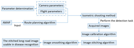
Figure 1.
The general framework of UAV road damage detection in this study.
2.2. Determination of UAV Parameters
2.2.1. Camera Parameters
During image acquisition, in order to not affect any vehicles on the road, a camera height of at least 5 m from the road should be maintained. At the same time, in order to reduce the distortion of the road image, it is also inadvisable to choose a wide-angle lens whose focal length is too short. Therefore, the lens used in this study is of 35 mm fixed focal length.
Furthermore, in order to ensure satisfying image stitching results, it is necessary to ensure that the lens is perpendicular to the road when shooting. Therefore, the pitch angle of the UAV was set to 0° and the pitch angle of the gimbal(camera) to 90° (perpendicular to the road) when shooting in this study.
2.2.2. Minimum Requirements for Image Pixels
When the UAV performs a road surface detection task, its flight altitude will determine the proportion of the detected road in the image. Field tests in this study show that, for road images, the feature points extracted by the image-matching algorithm are often concentrated on trees, plants, green belts and other roadside facilities on both sides of the road, and it is difficult to extract features from the road itself. In order to facilitate image stitching, a certain net width needs to be maintained on both sides of the road when acquiring images; or, in other words, the image range should be larger than the road range. The lateral width of the image range can be calculated by the Equation (1):
where b represents the lane width, n represents the number of lanes, and a represents the net width maintained on both sides of the road.
According to previous research [34], the success rate of pavement disease identification is highly dependent on the definition of the image. A road image of 100 × 100 pixels or 200 × 200 pixels is usually needed for machine learning and pavement disease recognition. To guarantee the success of crack identification in a 50 cm × 50 cm road surface region, an image of 200 × 200 pixels will be needed, if the crack is relatively mild. According to this, the demand of image definition is identified as 2.5 mm/pixel. When the lateral width of the image range is fixed, the definition of the road surface image could be calculated by Equation (2):
where is the aspect ratio of the image.
According to Equations (1) and (2), the required lateral width for various road widths, as well as the definitional demands of the road images, are listed in the Table 1:

Table 1.
Recommended minimum pixel values for various road widths.
2.2.3. Minimum Requirements for Flight Altitudes
According to the lens imaging principle of the camera vision system, the relationship between the lateral width of the image range and the focal length of the lens can be expressed through Equation (3):
where is the distance between the sensor and the photographed object, which is also the flight height in this study, while is the lateral width of the sensor in the camera, and is the focal length of lens. According to Equation (3), the flight height could thus be calculated by the Equation (4):
The length of the sensor in the camera used in this study is 36 mm, and the focal length of the lens is 35 mm. The suggested flight heights of the UAV are listed in Table 2:
Table 2.
Recommended flight heights for various road widths.
2.2.4. Optimal Equidistant Shooting Intervals
The images collected by the UAV are continuous single images, which need to be stitched to form a complete long image of the pavement. If the image overlap ratio is too low while the images are being stitched together, this will affect the accuracy of the matching algorithm and will thus cause distortion in the final image. Figure 2 shows that, when the overlap ratio is low, a large offset angle () may be caused in the stitched image. On the other hand, an excessively demanding image overlap rate will occupy too much memory resources and increase the calculation cost.
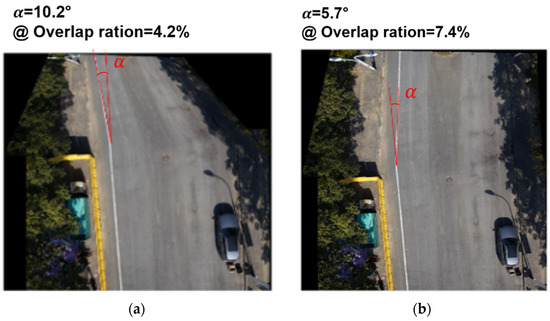
Figure 2.
The distortion (at large offset angles ()) of the stitched image when the overlap ratio is low. (a) The stitched image when the overlap ratio is 4.2% and (b) the stitched image when the overlap ratio is 7.4%.
To obtain an optimal overlap ratio, one that guarantees the quality of the stitched image while incurring the lowest possible calculation cost, and thus further calculate the optimal shooting interval distance, a series of image stitching experiments were conducted in this study. The relationship between the overlap ratio and the offset angle of the stitched image is shown in Figure 3:
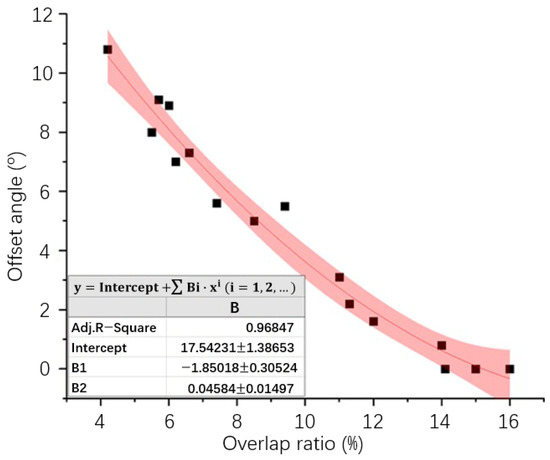
Figure 3.
The relationship between the overlap ratio and the offset angle.
As can be seen from Figure 3, when the overlap ratio reaches 15% or more, the offset angle of the stitched image will drop to 0°, i.e., no distortion will occur. Previous research [35] has also proved that, when the overlap ratio is larger than 20%, the stitching result is satisfactory. Considering the above conclusions, the overlap ratios adopted in this study are between 20% and 25%.
Similar with Equation (4), the longitudinal width of the image range can be calculated by Equation (5):
where is the longitudinal width of the sensor in the camera, which is 24 mm in this study. The calculation results of equidistant shooting intervals are listed in the Table 3:
Table 3.
Recommended equidistant shooting intervals for various road widths.
2.2.5. Recommended Shutter Speeds
According to the previous study [36], The longest shutter time can be calculated by Equation (6):
where is the camera distance, which is the flight height in this study, is the diameter of the dispersion circle, which is 0.033 mm in this study, and is the speed of object movement relative to the camera, which is the flying speed of the UAV in this paper.
According to Equation (6), the longest shutter times were calculated and are listed in Table 4:
Table 4.
Recommended longest shutter time for various roads and flying speeds.
Considering that an asphalt road is a dark object compared with the surrounding environment, to guarantee the success of asphalt road disease identification, the image should not be too dark. The issue of the brightness of the image is essentially a matter of exposure. In addition, camera parameters, such as aperture, exposure mode, sensitivity and white balance, also have an effect on the brightness of the image. Furthermore, the ambient light intensity, shooting angle and color temperature will also have an effect on the image. In this paper, other factors affecting the brightness of the captured road images will not be further studied, as only the influence of the shutter time was investigated.
A shorter shutter time usually leads to a lower image brightness, as shown in Figure 4 where the brightness of the image whose shutter speed was 1/1200 s is significantly lower than that of the image whose shutter speed was 1/800 s. In general, the shutter speed of 1/800 s can ensure both the sufficient brightness and clarity of most urban road and highway images, so the shutter speed adopted in this study is 1/800 s.
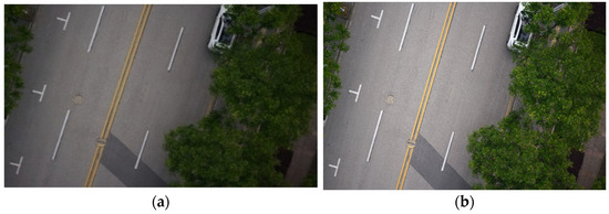
Figure 4.
The road images obtained with different shutter speeds: (a) shutter speed of 1/1200 s and (b) shutter speed of 1/800 s.
2.2.6. Recommended Flying Speed
The fastest flying speed of the UAV in this study is mainly dependent on the maximum shooting frequency and shooting interval:
The minimum shooting time interval is 1 s in this study. The fastest flying speed of the UAV can thus be calculated according to Table 4, and is listed in Table 5. Since there is no upper limit for the shooting time interval, the fastest flying speed of UAV is set as 5 m/s under all the conditions except for the one-lane road condition (under which the fastest flying speed is 3.87 m/s).
Table 5.
Recommended fastest flying speeds for various road widths.
2.3. The UAV Control Method for Road Performance Testing
2.3.1. The Route Planning Method Based on the Modified Dijkstra Algorithm
The route planning task refers to the task of deciding the best route based on the given planning space under certain constraints and presenting the planned route in a certain form. The basic process of the route planning algorithm can be divided into the following key steps:
- (1)
- The planning space description:
Since the movement route of the actual object is planned according to the traffic network, it is necessary to match the real geographical environment with the abstract simulation environment of the computer, that is, to build a world in the “computer’s eyes”. The common methods are the raster and the graph methods. In the raster method, the planning space is divided into several grids, then the intensity and density of obstacles in these grids are expressed by the pass cost. In the graph method, the planning space is composed of nodes and weighted undirected line segments. The weight can represent the cost of passage, and the higher the cost, the more difficult the passage between nodes.
- (2)
- The constraints determination:
There are many trajectories that consume more time or resources, thus not all trajectories are worth being realized in the real world. At the same time, the real situation is more complex than the abstract simulation, so it is necessary to screen the trajectories through constraints. For the UAV flight route in this study, the flight height should be stable at a fixed value because the prime lens is used, and the yaw angle and depression angle of the UAV have maximum limits to ensure safety. Therefore, these constraints should be taken into account when planning and screening trajectories.
- (3)
- Cost evaluation:
The cost function K is mainly composed of path length cost L, obstacle cost B and height cost H. Since this study does not consider the change of height, the final K function could be described as in Equation (8):
where s is the result of route calculation, which is usually a linear table, and and represent the weights of the path length cost and obstacle cost, respectively. In road detection tasks, UAVs usually perform tasks directly above the road, thus obstacles such as buildings or trees on either side of the road do not affect the route calculation, which means L has a larger weight than B, and that is thus ignored in this study.
- (4)
- The route calculation:
On the basis of planning space and cost evaluation, the next step is to calculate the minimum cost route according to the given constraints, which is also the core of the whole route planning algorithm.
- (5)
- The determination of the result form:
Once the route calculation result corresponding to the minimum cost is obtained, it needs to be resolved into path information in a form which is understandable by the users, such as route equation, waypoint, etc. In order to reduce and adjust the algorithm cost, waypoint representation has been chosen for this study. The waypoint representation mode is the official flight mission execution mode of DJI, so it is easy to import into the UAV flight control system, and the execution time and accuracy of the algorithm can be adjusted by controlling the number of generated waypoints.
The commonly used wireless communication range of commercial UAVs is within 1 km, so if it is beyond this range, it would be easy to lose contact and crash. The range of the single road detection task is not very large because of this limitation. Therefore, in the route calculation step, the basic and relatively simple optimized Dijkstra algorithm has been selected for this study.
The Dijkstra algorithm can calculate the shortest path from a node to any other node in the graph. Once a positive weighted directed graph is input, the algorithm can correctly calculate the shortest path of any two nodes in the graph, thus the Dijkstra algorithm is a deterministic algorithm. A positive weighted directed graph could be usually described as , where V is the node set in the graph, and A is the matrix which describes the line set. In a traffic network, the weight refers to the length of line l which links node v and node w, and a route P could be represented as a set of several nodes, , so that the length of route P could be described as: . The aim of the algorithm is to find the shortest route and the shortest length between the given two points s and t.
A mathematical model of a traffic network can be represented as a node set V and a matrix A which describes the line set. In the node set , each node is assigned a number by subscript. In the matrix A, the element is the weight value of the line between node and node , which could also be represented as . If there are no lines to link the two nodes, the symbol can be used. The basic principle of the Dijkstra algorithm is to start from an initial node, to successively include nodes into the path according to the shortest path principle, and to use a table to record the added nodes until the shortest path of all the nodes is generated. For example, for the abstract traffic network shown in Figure 5, the process of the Dijkstra algorithm could be concluded in Table 6, where the orange cells represent the shortest flight route derived by the algorithm.

Figure 5.
The abstract traffic network.
Table 6.
The process of the Dijkstra algorithm.
The Dijkstra algorithm implements the greedy strategy and adopts the double-loop method to gradually expand the scale of the problem. In the algorithm, there are three assistant tables: , , and . For the node and the initial node , the table is used to store the distance between the initial node and the node . If there are no pathways between those two nodes, the distance would be . is used to record the previous node on the shortest route between and for the backtracking after comparison. is used to record whether node has already been concluded in the shortest route.
The whole algorithm can be divided into two loops. The outside loop extracts from , sets as 0, then the inner loop traverses all nodes to check whether has already been in the table , if not, then it checks whether the new node will make the original route shorter, which is to compare the length of and . If the new route is shorter, then it updates the new shortest route and adds node into the shortest route. In practice, only the shortest route from the initial node to a certain target node is needed, so it is necessary to add the specific condition to stop the loop, that is, once is 1, the algorithm should be terminated immediately.
The disadvantage of the Dijkstra algorithm is that the time complexity will increase rapidly once the scale of nodes in the problem increases. Therefore, for large-scale problems, in order to simplify the problem, it is necessary to rewrite the original traffic network diagram without changing its traffic logic [37].
The raster method is usually used to model the traffic network in the road database. The raster cuts the road into several small segments, with each segment regarded as two nodes and a line in the algorithm. When the UAV flies along the actual road, some sections of the road will be less curved than others, therefore requiring less nodes, as is shown in Figure 6. Therefore, a specific strategy [38] to omit those unnecessary nodes has been adopted in this paper to maintain the scale of the Dijkstra algorithm and to reduce the time and memory cost.
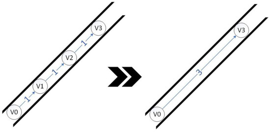
Figure 6.
The removal of unnecessary nodes.
To omit the unnecessary nodes, we must first, from the initial node, traverse the node set by the layer sequence to check the sub-line set where all the lines with a point as the end are temporarily stored in the table . Then, all sub-line sets of the nodes at the next layer are checked. The elements in these sub-line sets are to be potentially merged with the lines in . If the three-point connection angle is greater than 103°, then their corresponding lines must be merged into a shortcut line, as shown in Figure 6.
Since DJI MobileSDK is the only route navigation execution method provided by the official open-source library of DJI, the DJI MobileSDK with WayPointMission was adopted to realize the control of UAV by route planning algorithm in this paper. The positive weighted directed graph required by the input of the route planning algorithm was obtained from AMAP. It has been proved that the route planning method based on the modified Dijkstra algorithm introduced above can complete a 5 km route plan for a UAV within 5 s, which meets the application requirement.
2.3.2. The Control Method of Continuous Image Acquisition at Equal Distances
The Callbacks function provided by the DJI client can be used to read the speed information of the UAV, as shown in Figure 7. In the flight process, at the beginning of each flight segment the UAV adjusts its heading so as to face the best direction in which to fly toward the end point from the starting point (which is the end point of the previous flight segment), and then accelerates to the end point (which is the starting point of the next flight segment) of the current flight segment. In the process of flight, the UAV first accelerates to the optimal speed, then flies at a constant speed, and slows down to 0 continuously when approaching the end point. When the flight segment is not long enough, there would be no constant speed flight process (as is shown in the red circles in Figure 7). The speed of the UAV is therefore not constant when flying along a curved road, indicating that the equal distance shooting mode, rather than the equal time interval shooting mode, should be adopted when taking pictures in UAV road continuous image acquisition tasks.
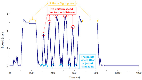
Figure 7.
The speed profile of the UAV during flight.
The core idea of the isometric shooting mode is the integral method, as shown in Figure 8. The y axis represents the speed of the UAV, the x axis represents time, and the area between the curve and the x axis represents the UAV’s flight distance. When the time interval is small enough, the areas of the rectangles will add up to a distance which is very close to the real flight distance. In this study, the selected time interval is 0.1 s, and the flight distance of the UAV is calculated by adding the rectangular areas. When the flight distance reaches the threshold (shooting interval), a picture will be taken, and then the distance will be reset to 0 for the distance calculation of the next picture. The process of the isometric shooting can be summarized in Figure 9.
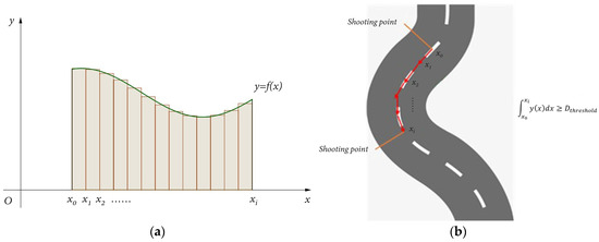
Figure 8.
The principle of the isometric shooting method: (a) the principle of integral method and (b) the actual UAV integral path along the road.
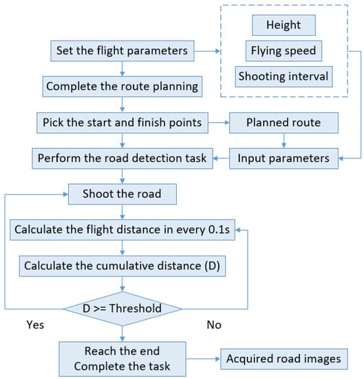
Figure 9.
The process of the isometric shooting method.
2.4. The Road Images Splicing Method
2.4.1. The Preprocessing Method of Road Images
In the road image acquisition tasks, if the road is wide and the acquisition camera is of high definition, the UAV will take pictures at a large angle. At this time, if the focal length of the camera lens is short, it is easy for barrel or radial distortions to appear. Most of the lenses carried by ordinary UAVs are non-professional photography lenses with a small focal length and easily produce optical distortions. After the road image is obtained, the image distortion needs to be calibrated for the subsequent image stitching. The most commonly used method for image distortion calibration is to obtain intrinsic and extrinsic matrixes by using the Zhang Zhengyou camera calibration method [39], and then adjusting the pixels of the image with the back-calculation method according to the intrinsic matrix.
Image deformation includes mainly radial and eccentric distortions. Previous research [40] has shown that the radial distortion is the main part of the optical distortion, while the eccentric distortion is only 1/7 to 1/8 of the radial distortion. Furthermore, when the radial distortion is eliminated, the influence of the eccentric distortion can also be alleviated, so the eccentric distortion can be ignored in the image calibration. The image distortion model can be expressed as Equations (9) and (10):
where and are the pixel-point displacements caused by image distortion, is the coordinate of the main point of the image (the intersection of the optical axis of the camera with the image plane), and are the radial distortion coefficients, and are the tangential distortion coefficients, refers to the parameters of the lens.
To determine the distortion coefficients of the camera, the camera calibrator in MATLAB_R2020a was used in this study. As for the calibration plate, a plate in the form of a checkerboard was adopted, one composed of 16 × 16 black and white squares alternating with each other, and with a side length for each square of 13 mm. The camera and the calibration plate are shown in Figure 10:
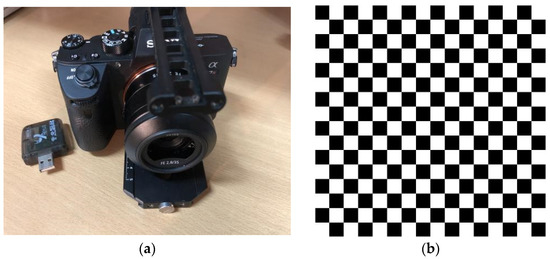
Figure 10.
The camera and the calibration plate adopted in this study. (a) The camera attached to the UAV and (b) the calibration plate in the form of a checkerboard.
2.4.2. The Road Images Splicing Method
At present, the most commonly used feature point extraction methods include the scale invariant feature transform (SIFT) method, the speeded-up robust features (SURF) method, the Harris corner point method, the features from accelerated segment test (FAST) method, etc. [41]. The SURF method was adopted in this paper to conduct the feature point extraction and image registration because of its advantages of stability, distinctiveness, quantity, high speed and expansion. The basic principle of the SURF method is similar to the SIFT method, and can be concluded as follows:
- (1)
- The detection of the extremum in the scale space.
Firstly, continuous down-order sampling is carried out on the images. All the obtained images are arranged layer by layer according to their size, the original image is placed at the bottom layer, and the size of the upper image decreases successively. Thus, the images would be arranged in the form of pyramid, as shown in Figure 11a. At the same time, the difference of gaussian (DOG) function is generated with the convolution and gaussian difference kernel of images of different scales. Then, for each pixel in the image, the pixel point is compared with all the other pixel points in the scale space and image space. If its value is larger than or smaller than all the surrounding points, then this point is regarded as the extreme point in the DOG space, and the extreme points are regarded as the feature points of the image. The comparison within the same scale ensures the existence of extreme points in the two-dimensional image space, while the comparison at different scales ensures the existence of extreme points in the scale space.
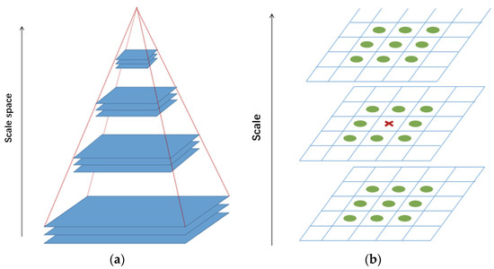
Figure 11.
The Gauss pyramid and extreme value detection. (a) Gauss pyramid and (b) extreme value detection in DOG space.
- (2)
- The precise positioning and principal direction assignment of feature points.
The fitting of a 3D quadratic function was adopted to precisely position and measure the feature points obtained in step (1). The pixel gradient amplitude and pixel gradient direction could be calculated as Equations (11) and (12):
where is the value of the scale space, and is the coordinate of the pixel. The gradient histogram and orientation histogram which contain the orientation and gradient information of pixels can be obtained with the calculation results. The peak value of the gradient histogram refers to the principal direction of the feature point, while the peak value of the direction histogram refers to the direction of the neighborhood gradient at the feature point.
- (3)
- The description of feature points.
To ensure that the feature points will not be affected by the disturbance of external factors, such as the change of illumination condition or angle of view in subsequent processing, descriptors are established for each extracted feature point. The descriptor of a feature point includes the feature point itself and all the contributing pixels around it. The image area around the feature point is divided into blocks, and the unique vector is generated by calculating the gradient histogram in each small block. The obtained vector can abstractly represent the image information in the corresponding region and is regarded as the descriptor.
- (4)
- The matching of feature points.
The descriptor sets of the feature points (which is of 128 dimensions) for both the reference image (template image) and observed image (real-time image) are established. The descriptor of feature points in the reference image is , while that of the real-time image is . The similarity between any two descriptors is measured with Euclidean distance , and the feature point descriptors are matched when . Where is the closest point to in the real-time image, and is the second closest point to in the real-time image.
To solve the problem of high mismatch rate in image matching, the random sampling consistency (RANSAC) algorithm [42] was used in this paper to eliminate the incorrect matching pairs. After the incorrect matching pairs are eliminated, the transformation matrix T of the connecting image relative to the basic image should be calculated, the image should then be affine transformed according to the T matrix to ensure that the connecting part is smooth. Affine transformation is a two-dimensional projection that maps points in one plane to another plane, including translation, rotation, scale transformation and so on. Affine transformation maintains the “flatness” of two-dimensional graphics and has high practicability, being used for image matching, image correction, texture correction, creating panoramic images, etc. The mathematical expression of affine transformation is given in Equation (13):
where the corresponding homogeneous coordinate matrix is:
After the affine transformation process, the coordinates of pixels of different images are mapped to the same world coordinate system. With all the pixels displayed in the world coordinate system, the final, spliced image can be shown.
2.4.3. The Smoothing Method for Spliced Images
If the images are simply connected together, uneven brightness around stitching seams will occur, as shown in the red circles in Figure 12, and will greatly affect the recognition of pavement diseases. Therefore, the brightness of pixels at the junction should also be adjusted after the image stitching process is completed. Thus, the optimize gradual in and out weight fusion method was used in this paper to eliminate the unevenness between light and dark parts.
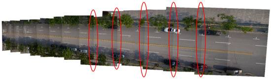
Figure 12.
The stitched road image without smoothing process.
The basic principle of the optimize gradual in and out weight fusion method is that the original image and the image to be matched are given the same weight, and the pixel value at the joint is taken as the weighted average of the pixel values of the two images, so as to realize the smooth transition of the joint of the stitched image [43].
To eliminate the uneven part of light and dark in the stitched image, the range of the image placed in the world coordinate system after image registration is calculated first. Then the biaxial range of the two images is compared to obtain the range of the overlap in the world coordinate system. On this basis, the mask matrix sub-information with the same size as the two images is established. In the mask matrix, the value of the non-overlapping area is 1, and the value of the overlapping area gradually decreases from 1 to 0 from the non-overlapping area to the edge. The establishment and structure of the mask matrix are shown in Figure 13. The three channels of the two color images are dotted with the mask matrix, and finally placed in the world coordinate system. The overlapping regions cover each other directly, and then the smooth stitched image is obtained.
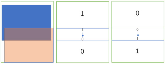
Figure 13.
The mask matrix.
3. Results
3.1. The Test of UAV Control Method
The UAV control method developed in this paper was tested on a straight road and a curved road. The path planning results of the path planning algorithm for two roads are shown in the Figure 14:
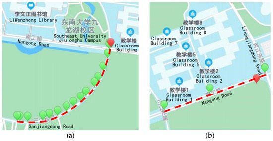
Figure 14.
The test roads. (a) The curved test road and (b) the straight test road.
It can be seen from Figure 14 that the route planning algorithm has good route calculation ability. For the route on the curved road in Figure 14a, 12 waypoints were given (excluding the start and end points), while for the route on the straight road, few waypoints were given, which means that the division of the curved section is more accurate, and the division of the straight section is rougher. This indicates that the algorithm proposed in this paper can dynamically adjust the accuracy of the calculation results according to the actual road alignment, so the algorithm has good robustness.
The real-time status parameters of the UAV, including longitude and latitude coordinates at 0.1 s intervals, were obtained through callback function, so that the actual flight route of the UAV could thus be obtained. The planned route and real flight route are drawn in the Figure 15, where the red line is the planned route given by the algorithm, and the black line is the actual flight route of the UAV.
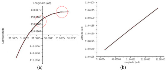
Figure 15.
The comparison of planned and actual routes. (a) The curved route and (b) the straight route.
For the curved road, it can be seen that most of the trajectories of the UAV’s actual flight overlap with the planned route, but there are still some offsets, such as the areas marked in Figure 15a. The reason for the offset is mainly because the AMAP map uses the GCJ02 coordinate system, while the UAV uses the WGS84 coordinate system in flight. Therefore, the results of the AMAP-based route planning algorithm need to be converted by coordinates before they can be used for control of the UAV’s route. Additionally, the coordinate conversion will produce accuracy loss and when there are more waypoints, the accuracy loss will be more obvious. In the straight road, the actual UAV trajectories almost completely overlap with the planned route because there are fewer waypoints.
By reading the attribute information of the road images taken by the UAV, the coordinates of the shooting position of each image could be obtained. The shooting points were then plotted in the map, as is shown in Figure 16. From this, it can be seen that each image was taken at the same interval.
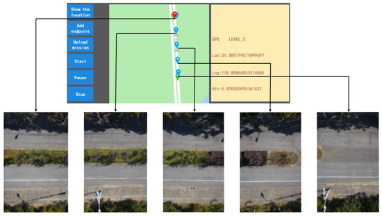
Figure 16.
The shooting points in field test.
3.2. The UAV Flight Parameters Testing
Three road sections with different road widths were selected for UAV image acquisition tests in this study. The weather conditions at the time of testing were clear and breezy. As is described in the Section 2.2.2, the camera was of 60 megapixels, and the flight parameters during image acquisition were determined according to Section 2.2.
Test 1 is the image acquisition test on a three-lane road. According to the conclusions in Section 2.2, the parameters selected for the image acquisition process are listed in Table 7.
Table 7.
The parameters for a three-lane road.
The results for continuous road image acquisition at equal distance intervals is shown in Figure 17, and the image is partially enlarged as shown in Figure 18.
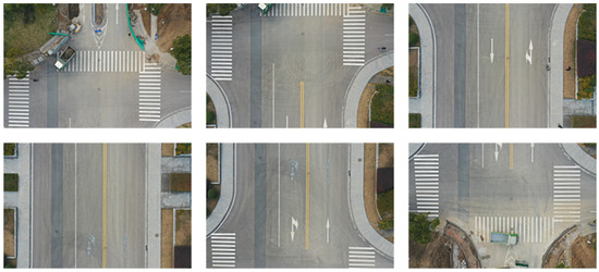
Figure 17.
The isometric shooting results for the three-lane road.
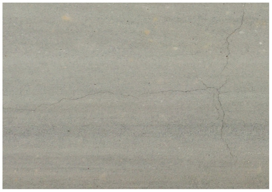
Figure 18.
The partially enlarged image of the three-lane road.
Test 2 is the image acquisition test on a two-lane road. The parameters selected for the image acquisition process are listed in Table 8:
Table 8.
The parameters for a two-lane road.
The results for continuous road image acquisition at equal distance intervals is shown in Figure 19, and the image is partially enlarged as shown in Figure 20.
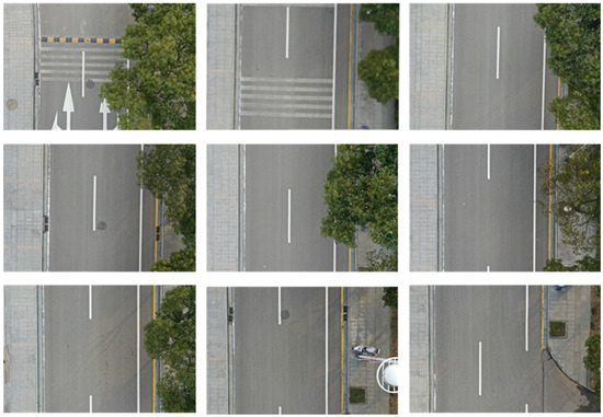
Figure 19.
The isometric shooting results for the two-lane road.
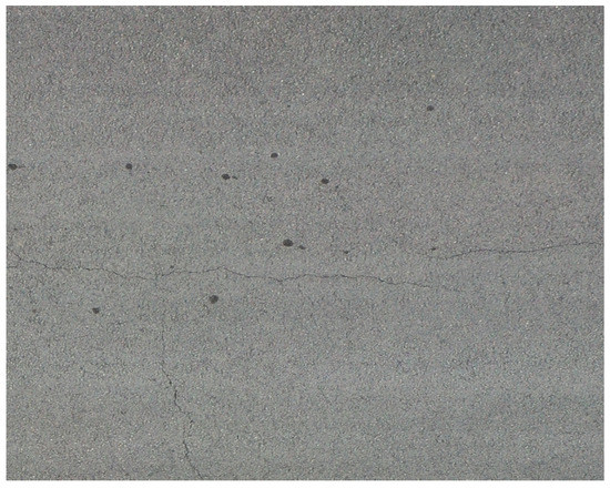
Figure 20.
The partially enlarged image of the two-lane road.
Test 3 is the image acquisition test on a six-lane road. The parameters selected for the image acquisition process are listed in Table 9:
Table 9.
The parameters for a six-lane road.
The results for continuous road image acquisition at equal distance intervals is shown in Figure 21, and the image is partially enlarged as shown in Figure 22.
Figure 21.
The isometric shooting results for the six-lane road.
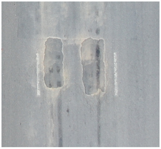
Figure 22.
The partially enlarged image of the six-lane road.
From the above results, it can be found that the ranges and the net widths calculated by the method developed in Section 2.2 meet the requirement of covering the whole pavement surface. Furthermore, the cracks and other diseases could also be identified clearly from the images, which indicates that the definitions of the images obtained in the three tests also meet the requirements of pavement disease identification.
3.3. The Road Images Processing Result
3.3.1. The Feature Point Extraction and Matching Result
As an optimized version of the SIFT algorithm with improved robustness, the SURF algorithm was used in this study to extract and match the feature points. The MATLAB toolbox function detectSURFFeatures was called to extract the feature points in the image, and the extractFeatures function was called to establish the feature point descriptors. The result of feature extraction is shown in Figure 23:
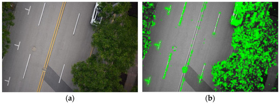
Figure 23.
The result of feature extraction. (a) original image and (b) extracted feature points.
The coarse matching of feature points between two images was achieved by the matchFeatures function. Two sets of feature point vectors were inputs, and the function returned the matched point pairs. The coarse matching result is as shown in the Figure 24:

Figure 24.
The coarse matching result.
There are many wrongly matched pairs as a result of the matchFeatures function, which will significantly influence the accuracy of the conversion matrix calculation and image stitching. The estimateGeometricTransform function, which is based on the RANSAC algorithm, was used to eliminate the wrongly matched pairs and calculate the transformation matrix. The matching result after the modification of estimateGeometricTransform function is as shown in Figure 25, in which all the wrongly matched pairs were eliminated.
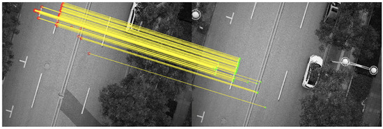
Figure 25.
The modified matching result.
3.3.2. The Image Splicing Result
The result of multiplying the pixel values of the RGB trichromatic channels with the mask matrix is shown in Figure 26, and the final stitched image is shown in Figure 27. The images were stitched accurately to each other without uneven brightness around the stitching seams, which indicates that the image splicing and smoothing methods in this study are valid.
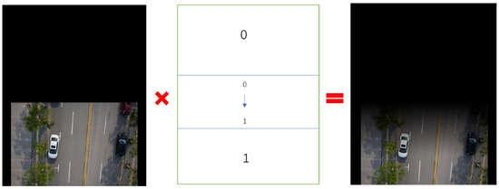
Figure 26.
The image after mask matrix processing.
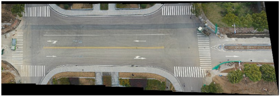
Figure 27.
The final stitched image.
3.3.3. The Image Smoothing Result
The aim of this study is to provide a feasible image acquisition method for UAV pavement disease detection, so it is necessary to make sure that the aerial pavement long images acquired by the above algorithm can be applied to machine learning for pavement disease identification. A prerequisite for the successful use of the stitched image so that machine learning can be used to identify cracks is that the pavement cracks in the stitched image can be clearly displayed. Zooming in and observing Figure 27, four crack damage areas can be clearly identified, as is shown in Figure 28.
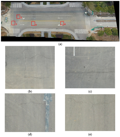
Figure 28.
The disease recognition in the stitched image. (a) The location of the four diseases, (b) disease 1, (c) disease 2, (d) disease 3, and (e) disease 4.
When machine learning is used to identify pavement diseases, an important step is to extract the morphology and dimensions of the object of the disease, i.e., to establish an effective training library of pavement disease models. The most common methods used in morphology and dimension extraction operations of diseases is edge detection processing. There are two common edge detection operators, Canny and Otsu [44,45,46], among which the Canny operator works better for square pictures [47].
The stitched images without smoothing process will greatly affect the extraction of disease objects in the Canny operator due to the uneven brightness at the junction, as is shown in Figure 29. In Figure 29b, due to the uneven brightness around them, the stitching seams were also extracted by the Canny operator into the edge detection result, which could be easily misidentified by machine learning as pavement transverse cracks. In order to test whether the stitched images after the smoothing process in this paper would still have an effect on the extraction of disease objects, the extraction of disease objects by Canny was conducted on the stitched images after the smoothing process, as shown in Figure 30. After the smoothing process, the stitching seams were no longer extracted by the Canny operator as edges, while the cracks on the road surface were still successfully extracted. This means that the long road stitched image obtained by the image stitching and smoothing method in this paper can be applied for machine learning recognition and evaluation of pavement distress, and that the UAV road surface image continuous acquisition method developed in this paper is valid and can be applied in the future practical application of UAV pavement disease detection tasks.
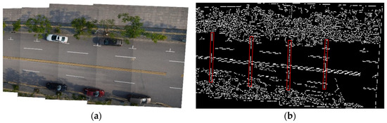
Figure 29.
Disease object extraction in unsmoothed image. (a) The unsmoothed stitched image and (b) the disease object extraction result.
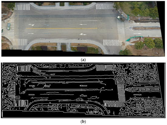
Figure 30.
The disease object extraction in smoothed image. (a) The smoothed stitched image and (b) the disease objects extraction result.
4. Conclusions
Due to the demand for UAV pavement disease detection, this paper studied and determined the suggested values of camera parameters and flight parameters for UAV continuous road image acquisition tasks, and proposed the UAV flight route planning method, continuous photography control method and image stitching and smoothing processing method for road disease detection tasks. The following conclusions can be made:
- In the UAV road disease detection tasks, the image overlap ratio should be guaranteed to be above 15%, and it is recommended to be between 20% and 25%. The lateral width of the image range should be between 7.75 m and 26.5 m according to the width of the road, the longitudinal width of the image range should be between 5.16 m and 17.67 m. Camera pixels are recommended to be between 5.6 million and 62 million, flight height should be between 7.6 m and 26 m, shutter speed should be controlled between 1/800 s and 1/1200 s, and the flight speed is recommended to be 3.5 m/s or 5 m/s. The exact values of the parameters should be determined by the number of lanes and the width of the road.
- The route planning method based on the modified Dijkstra algorithm proposed in this study can complete a 5 km route plan for a UAV within 5 s, which meets the application requirement. With the continuous image acquisition method, the UAV can fly along the road median and take road pictures at equal distance automatically.
- Based on the correction of camera optical distortion using Zhang Zhengyou’s camera calibration method, a road image stitching method using SURF and RANSAC algorithm to extract and match feature points, an affine transformation to stitch the road long image, and an optimized gradual in and out weight fusion method to smooth the stitched image were all proposed in this paper. The stitched road long image obtained with this method is applicable for machine learning of asphalt pavement disease identification based on the Canny edge extraction method.
There are still some limitations in this study, such as the impacts of camera exposure mode, aperture setting, sensitivity, white balance and other parameters that were not considered in the determination of the shutter speed. Furthermore, the impact of natural lighting conditions was also not considered. In addition, the question of how to add obstacle avoidance algorithms into the route planning method to enhance the flight safety in automatic UAV pavement disease detection tasks was also not considered in this paper. Therefore, the question of how to more comprehensively consider the shutter speed to ensure image brightness, as well as of how to optimize the route planning algorithm to further ensure the safety of the UAV’s flight are recommended to be the focus of research in the future.
Author Contributions
Conceptualization, R.Z. and Y.H.; methodology, H.L.; validation, R.Z.; formal analysis, R.Z.; investigation, Y.H.; resources, X.H.; writing-original draft preparation, R.Z.; writing-review and editing, H.L., X.H. and Y.Z.; visualization, R.Z. and Y.H.; supervision, X.H.; project administration, X.H. All authors have read and agreed to the published version of the manuscript.
Funding
This research was funded by the NATIONAL KEY R&D PROGRAM OF CHINA, grant number 21YFB2600600 and 21YFB2600601.
Institutional Review Board Statement
Not applicable.
Informed Consent Statement
Not applicable.
Data Availability Statement
The data used to support the findings of this study are included within the article.
Conflicts of Interest
The authors declare no conflict of interest.
References
- Naseri, H.; Golroo, A.; Shokoohi, M.; Gandomi, A.H. Sustainable pavement maintenance and rehabilitation planning using the marine predator optimization algorithm. Struct. Infrastruct. E 2022, 1–13. [Google Scholar] [CrossRef]
- Bogus, S.M.; Song, J.; Waggerman, R.; Lenke, L.R. Rank Correlation Method for Evaluating Manual Pavement Distress Data Variability. J. Infrastruct. Syst. 2010, 16, 66–72. [Google Scholar] [CrossRef]
- Bianchini, A.; Bandini, P.; Smith, D.W. Interrater Reliability of Manual Pavement Distress Evaluations. J. Transp. Eng. 2010, 136, 165–172. [Google Scholar] [CrossRef]
- Bogus, S.M.; Migliaccio, G.C.; Cordova, A.A. Assessment of Data Quality for Evaluations of Manual Pavement Distress. Transport. Res. Rec. 2010, 2170, 1–8. [Google Scholar] [CrossRef]
- Guide for Design of Pavement Structures; American Association of State Highway and Transportation Officials (AASHTO): Washington, DC, USA, 2002.
- Pan, Y. Principle of Pavement Management System; People’s Communications Press: Beijing, China, 1998. [Google Scholar]
- Fukuhara, T.; Terada, K.; Nagao, M.; Kasahara, A.; Ichihashi, S. Automatic Pavement & Distress & Survey System. J. Transp. Eng. 1990, 116, 280–286. [Google Scholar]
- Wang, K.C.P. Designs and Implementations of Automated Systems for Pavement Surface Distress Survey. J. Infrastruct. Syst. 2000, 6, 24–32. [Google Scholar] [CrossRef]
- Kaul, V.; Tsai, Y.J.; Mersereau, R.M. Quantitative Performance Evaluation Algorithms for Pavement Distress Segmentation. Transport. Res. Rec. 2010, 2153, 106–113. [Google Scholar] [CrossRef]
- Zhang, H.; Guo, D.; Chen, X.; Li, R.; Pei, J.; Zhang, J.; Cui, S. Indoor Study on Road Crack Monitoring Based on Polymer Optical Fiber Sensing Technology. J. Test. Eval. 2019, 49, 473–492. [Google Scholar]
- AL-Qadi, I.L.; Lahouar, S. Measuring layer thicknesses with GPR—Theory to practice. Constr. Build. Mater. 2005, 19, 763–772. [Google Scholar] [CrossRef]
- Lorenzo, H.; Rial, F.I.; Pereira, M.; Solla, M. A full non-metallic trailer for GPR road surveys. J. Appl. Geophys. 2011, 75, 490–497. [Google Scholar] [CrossRef]
- Wang, J.; Tang, J.; Chang, H. Fiber Bragg Grating Sensors for Use in Pavement Structural Strain-Temperature Monitoring—Art. In Proceedings of the of SPIE—The International Society for Optical Engineering, San Diego, CA, USA, 27 February–2 March 2006; p. 6174. [Google Scholar]
- Xu, D.S.; Luo, W.L.; Liu, H.B. RETRACTED: Development of a fiber Bragg grating sensing beam for internal deformation measurement in asphalt pavement. Adv. Struct. Eng. 2017, 23, P1–P8. [Google Scholar] [CrossRef]
- Atencio, E.; Plaza-Muñoz, F.; Muñoz-La Rivera, F.; Lozano-Galant, J.A. Calibration of UAV flight parameters for pavement pothole detection using orthogonal arrays. Automat. Constr. 2022, 143, 104545. [Google Scholar] [CrossRef]
- Guo, G.; Zhang, Z. Road damage detection algorithm for improved YOLOv5. Sci. Rep. 2022, 12, 15523. [Google Scholar] [CrossRef]
- Arya, D.; Maeda, H.; Ghosh, S.K.; Toshniwal, D.; Mraz, A.; Kashiyama, T.; Sekimoto, Y. Deep learning-based road damage detection and classification for multiple countries. Automat. Constr. 2021, 132, 103935. [Google Scholar] [CrossRef]
- Xiong, Y.; Lu, G.; Zhu, Z. Detection Technique of Distress Treatment Quality of Soft Foundation for Expressway. Highway 2007, 8, 81–84. [Google Scholar]
- Yu, Z. Reasonable Selection of Highway Subgrade and Pavement Disease Detection Technology. Highway 2007, 05, 19–23. [Google Scholar]
- Xue, P.; Jin, G.; Lu, L.; Tan, L.; Ning, J. The key technology and simulation of UAV flight monitoring system. In Proceedings of the 2016 IEEE Advanced Information Management, Communicates, Electronic and Automation Control Conference (IMCEC), Xi’an, China, 3–5 October 2016; pp. 1551–1557. [Google Scholar]
- Ma, T.; Yang, C.; Gan, W.; Xue, Z.; Zhang, Q.; Zhang, X. Analysis of technical characteristics of fixed-wing VTOL UAV. In Proceedings of the 2017 IEEE International Conference on Unmanned Systems (ICUS), Beijing, China, 27–29 October 2017; pp. 293–297. [Google Scholar]
- Rushdi, M.S.A.; Tennakoon, T.M.C.L.; Perera, K.A.A.; Wathsalya, A.M.H.; Munasinghe, S.R. Development of a small-scale autonomous UAV for research and development. In Proceedings of the 2016 IEEE International Conference on Information and Automation for Sustainability (ICIAfS), Galle, Sri Lanka, 16–19 December 2016; pp. 1–6. [Google Scholar]
- Pan, Y.; Zhang, X.; Cervone, G.; Yang, L. Detection of Asphalt Pavement Potholes and Cracks Based on the Unmanned Aerial Vehicle Multispectral Imagery. IEEE J. Stars 2018, 11, 3701–3712. [Google Scholar] [CrossRef]
- Li, Y.; Ma, J.; Zhao, Z.; Shi, G. A Novel Approach for UAV Image Crack Detection. Sensors 2022, 22, 3305. [Google Scholar] [CrossRef] [PubMed]
- Lin, Y.; Nie, Z.; Ma, H. Structural Damage Detection with Automatic Feature-Extraction through Deep Learning. Comput. Aided Civ. Inf. 2017, 32, 1025–1046. [Google Scholar] [CrossRef]
- Koziarski, M.; Cyganek, B. Image recognition with deep neural networks in presence of noise – Dealing with and taking advantage of distortions. Integr. Comput. Aid. E 2017, 24, 337–349. [Google Scholar]
- Salman, M.; Mathavan, S.; Kamal, K.; Rahman, M. Pavement crack detection using the Gabor filter. In Proceedings of the 16th International IEEE Conference on Intelligent Transportation Systems (ITSC 2013), The Hague, The Netherlands, 6–9 October 2013; pp. 2039–2044. [Google Scholar]
- Sorncharean, S.; Phiphobmongkol, S. Crack Detection on Asphalt Surface Image Using Enhanced Grid Cell Analysis. In Proceedings of the 4th IEEE International Symposium on Electronic Design, Test and Applications (Delta 2008), Hong Kong, China, 23–25 January 2008; pp. 49–54. [Google Scholar]
- Kang, W.; Xu, Y. A Hierarchical Dijkstra Algorithm for Solving Shortest Path from Constrained Nodes. J. South China Univ. Technol. 2017, 45, 66–73. [Google Scholar]
- Li, S.; Zhu, F.; Zhang, J.; Liu, J.; Sui, X. Multi-Restriction Path Planning Based on Improved A* Algorithm. Electron. Opt. Control. 2014, 21, 36–40. [Google Scholar]
- Yang, R.; Ding, Y.; Zhang, C. Application of the Improved A*Algorithm Based on DTW in Route Planning. Electron. Opt. Control. 2016, 23, 5–10. [Google Scholar]
- Guo, S.; Sun, X. Path Planning of Mobile Robot Based on Improved Particle Swarm Optimization. Electron. Meas. Technol. 2019, 42, 54–58. [Google Scholar]
- Jia, H.; Wei, Z.; He, X.; Zhang, L.; He, J.; Mu, Z. Path Planning Based on Improved Particle Swarm Optimization Algorithm. Trans. Chin. Soc. Agric. Mach. 2018, 49, 371–377. [Google Scholar]
- Huang, T. Research on Classification and Recognition of Asphalt Pavement Disease Image Based on CNN. Master’s Thesis, Chongqing Jiaotong University, Chongqing, China, 2019. [Google Scholar]
- Xiang, Y. Research on Image Registration Technology Based on Point Feature. Master’s Thesis, Northeastern University, Shenyang, China, 2010. [Google Scholar]
- Xu, S. Research on Motion Blur Image Deblurring Technology based on Computational Photography. Ph.D. Thesis, National University of Defense Technology, Changsha, China, 2011. [Google Scholar]
- Zhang, H.; Guan, A.; Fu, K.; Sun, Y. Experimental Study of Heap Optimization of Dijkstra Shortest Path Algorithm. Comput. Eng. Softw. 2017, 38, 15–21. [Google Scholar]
- Wu, H.; Wang, Y.; Yang, X. Analysis of Urban Traffic Vehicle Routing Based on Dijkstra Algorithm Optimization. J. Beijing Jiaotong Univ. 2019, 43, 116–121. [Google Scholar]
- Zhang, Z. Flexible camera calibration by viewing a plane from unknown orientations. In Proceedings of the Seventh IEEE International Conference on Computer Vision, Kerkyra, Greece, 20–27 September 1999; pp. 666–673. [Google Scholar]
- He, Z.; Ge, C.; Wang, C. Optical Lens Distortion Correction Method Based on Least Square Configuration. Chin. J. Liq. Cryst. Disp. 2019, 34, 302–309. [Google Scholar]
- Wang, Z. Research on the Technology of Electronic Image Stabilization based on Fast Feature Matching. Master’s Thesis, Nanjing University of Aeronautics and Astronautics, Nanjing, China, 2012. [Google Scholar]
- Yang, Q.; Ma, T.; Yang, C.; Wang, Y. RANSAC Image Matching Algorithm Based on Optimized Sampling. Laser Optoelectron. Prog. 2020, 57, 259–266. [Google Scholar]
- Xing, X. Research on Registration and Stitching Method of Remote Sensing Image. Master’s Thesis, Xi’an University of Science and Technology, Xi’an, China, 2020. [Google Scholar]
- Yang, J.G.; Li, B.; Chen, H.J. Adaptive Edge Detection Method for Image Polluted Using Canny Operator and Otsu Threshold Selection. Adv. Mater. Res. 2011, 301–303, 797–804. [Google Scholar] [CrossRef]
- Lang, B.; Shen, L.Y.; Han, T.; Chen, Y. An Adaptive Edge Detection Method Based on Canny Operator. Adv. Mater. Res. 2011, 255–260, 2037–2041. [Google Scholar] [CrossRef]
- Guiming, S.; Jidong, S. Remote sensing image edge-detection based on improved Canny operator. In Proceedings of the 2016 8th IEEE International Conference on Communication Software and Networks (ICCSN), Beijing, China, 4–6 June 2016; pp. 652–656. [Google Scholar]
- Cai, Z. Research on Automated Pavement Distress Detection Using Deep Learning. Master’s Thesis, Fujian Agriculture and Forestry University, Fujian, China, 2020. [Google Scholar]
Disclaimer/Publisher’s Note: The statements, opinions and data contained in all publications are solely those of the individual author(s) and contributor(s) and not of MDPI and/or the editor(s). MDPI and/or the editor(s) disclaim responsibility for any injury to people or property resulting from any ideas, methods, instructions or products referred to in the content. |
© 2023 by the authors. Licensee MDPI, Basel, Switzerland. This article is an open access article distributed under the terms and conditions of the Creative Commons Attribution (CC BY) license (https://creativecommons.org/licenses/by/4.0/).