Random Forest Algorithm for the Strength Prediction of Geopolymer Stabilized Clayey Soil

Abstract

Unconfined compressive strength (UCS) can be used to assess the applicability of geopolymer binders as ecologically friendly materials for geotechnical projects. Furthermore, soft computing technologies are necessary since experimental research is often challenging, expensive, and time-consuming. This article discusses the feasibility and the performance required to predict UCS using a Random Forest (RF) algorithm. The alkali activator studied was sodium hydroxide solution, and the considered geopolymer source material was ground-granulated blast-furnace slag and fly ash. A database with 283 clayey soil samples stabilized with geopolymer was considered to determine the UCS. The database was split into two sections for the development of the RF model: the training data set (80%) and the testing data set (20%). Several measures, including coefficient of determination (R), mean absolute error (MAE), and root mean square error (RMSE), were used to assess the effectiveness of the RF model. The statistical findings of this study demonstrated that the RF is a reliable model for predicting the UCS value of geopolymer-stabilized clayey soil. Furthermore, based on the obtained values of RMSE = 0.9815 and R² = 0.9757 for the testing set, respectively, the RF approach showed to provide excellent results for predicting unknown data within the ranges of examined parameters. Finally, the SHapley Additive exPlanations (SHAP) analysis was implemented to identify the most influential inputs and to quantify their behavior of input variables on the UCS.

1. Introduction

The mechanical, chemical, or biological improvement of the engineering characteristics of soil is known as soil stabilization. This is a method used in civil engineering to develop and enhance the engineering characteristics of soils [1,2]. These characteristics involve plasticity, durability, compressibility, permeability, and mechanical strength [3,4,5,6]. Mechanical or physical modification is common, but some researchers prefer to use the term ‘stabilization’ to refer to chemical modification in the soil characteristics by adding chemical additive materials. Stabilization is the act of combining and mixing different elements with soil to enhance certain soil qualities. The procedure could include combining commercially available additives to change the plasticity, texture, or gradation or serve as a binder for cementing the soil. Alternatively, it might involve blending soils to produce the appropriate gradation. In addition, for the soil to effectively sustain the stresses imposed by the superstructures, it is necessary to use soil stabilization procedures. This will ensure the necessary stability of the soil. Commonly, cement modification, which makes use of ordinary Portland cement (OPC), is employed in order to stabilize problematic soils via the utilization of chemical processes. However, throughout the last several decades, the use of OPC has been associated with various environmental problems, the most significant of which is the carbon footprint connected with the OPC building sector [7,8,9,10,11]. It is common knowledge that the production of OPC requires enormous amounts of energy, results in an excessive extraction of mineral materials, and causes the emission of high amounts of carbon dioxide (CO₂) into the atmosphere. OPC production is considered responsible for about 5 to 8% of the total CO₂ worldwide emission [12]. This problem has encouraged academics to design building binders that are less environmentally harmful and more sustainable. Geopolymer is a potential substitute for OPC since it is a synthetic alkali aluminosilicate material produced by reacting solid aluminosilicate [13,14] with hydroxide-silicate combination solution or concentrated aqueous alkali hydroxide. Its manufacturing method requires a lower total amount of fuel energy and generates a lower total amount of greenhouse emissions [11,15]. Geopolymers can be produced using a solid aluminosilicate derived from various industrial waste products, including silicate and/or alumina. These materials may be identified by their acronyms, such as ground-granulated blast-furnace slag (GGBS), metakaolin, and fly ash (FA) [16,17,18].

Turner and Collins [19] determined the amount of carbon dioxide equivalent emissions (CO₂-e) produced by all processes required to get raw materials, including concrete production. The assumptions depended on the activities involved in producing one cubic meter of Grade 40 concrete (for example, concrete with a compressive strength of 40 MPa) in the Melbourne Metropolitan area, which included the construction practices, manufacturing methods, and use of locally available materials. Sodium hydroxide with 16M concentration was the alkaline activator used in the geopolymers production. The geopolymer concrete emitted about 9% less CO₂ than conventional concrete with 100% OPC binder without any additives or replacement materials. This result was significantly lower than what was predicted by previous research. The inclusion of transport, treatment, and mining of raw materials in the manufacturing process of alkali activators for geopolymers, the expense of energy throughout the manufacturing process of alkali activators, and the requirement for higher curing temperatures for geopolymer concrete in order to gain sensible strength were the primary parameters that caused higher than predicted emissions for geopolymer concrete.

With the addition of fly ash or GGBS, soil improvement has been employed in geotechnical engineering projects [20,21]. Embankment works include building foundations, roads, dams, canals, and other similar structures [22,23,24]. According to findings from earlier studies, incorporating GGBS or FA into the soil may improve its mechanical strength [21,25,26,27]. The effectiveness of FA and GGBS in soil-stabilizing applications was studied by Sharma and Sivapullaiah [28]. GGBS and FA were assessed for the following curing times: 7, 14, and 28 days. After being allowed to cure for 28 days, the stabilized soil attained a strength of 0.45 MPa, and its plastic limit and water content values decreased. According to the results, utilizing GGBS and FA as binders offers a new opportunity for boosting pozzolan activity, potentially raising UCS and lowering clay soil swelling potential [25,26,27,28,29].

In general, determining the soft soil geotechnical parameters is a laborious, time-consuming, expensive, and energy-intensive process which involves a lot of time, work, and equipment. For instance, to obtain accurate data for determining the compaction characteristics and the UCS of soils, at least six and four tests need to be done, respectively.

Therefore, forecasting models have been developed to effectively predict the compaction parameters, UCS, and other soil properties. Traditional prediction methods for the UCS of stabilized soils are based on empirically derived relationships from statistical key parameters, using linear and non-linear regression approaches [30,31,32]. These approaches tend to generate equations with various undetermined coefficients that could impact the mappings of independent and dependent variables. Consequently, the resulting models are intrinsically erroneous despite being effective in some scenarios of stabilized soils, mainly because of their complexity.

Due to big data generation and data mining, Machine learning (ML) techniques and Artificial Intelligence (AI) are the appropriate choices for developing novel approaches that can address emerging challenges. For instance, models were developed by Suthar [33] for the UCS of lime sludge and stabilized pond ashes. The study evaluated the potential of five algorithms, including artificial neural networks (ANN), Random Forest (RF), Gaussian processes, support vector machines (SVM), and M5 model tree in terms of correlation coefficient (R), mean absolute error (MAE) and root mean square error (RMSE). For the test set, the Gaussian process model reported the lowest values of MAE = 16.455 and RMSE = 23.016 kPa, and the highest value of R = 0.997. Multi-gen genetic programming (MGGP) was employed by Soleimani et al. [34] to predict the UCS of geopolymer-treated clayey soil. The proposed MGGP model included multiple parameters affecting the soil UCS, including additive percentages, plastic limit, plasticity index, and others. The authors additionally carried out a parametric analysis to validate the employed models. The analysis revealed that the equations used to evaluate the UCS yielded good accuracy. Similarly, Support Vector Regressor (SVR) was employed by Mozumder et al. [35] to predict the shear strength of clayey soil Stabilized with geopolymer. The authors used 213 soil samples processed with geopolymer-based additives. The study revealed that SVR performs well in accurately predicting the shear strength of soil treated with geopolymer. Another study [36] employed Genetic Algorithm optimized SVR (GA-SVR) and ANN to predict the tensile strength (TS) and UCS of rocks in Bakken Field. The models outperformed other correlations regarding MAE, RMSE, and R². The study of Nagaraju and Prasad [37] examined the effectiveness of the particle swarm optimization (PSO) method in forecasting the 28-day UCS of expansive blended clays that have been alkali-activated. An accurate estimate using PSO is still achievable with the minimal experimental data currently available. Gullu [38] used several AI techniques to predict the UCS of soil stabilized with steel, jute fiber, and ash. A strong correlation between the AI algorithms employed and the estimated UCS value was indicated by the outcomes. Mathematical modeling for the UCS values of coal-grout composites was also conducted in [39] by using six ML models. SVM, decision trees (DT), and back-propagation neural network (BPNN) outperformed other models. Several studies highlighted the benefits concerning ML and AI techniques in the areas of road pavements as well as geotechnical engineering [40,41,42,43,44].

Although the UCS can be predicted using the models mentioned above, there is still room for improvement in accuracy. The RF algorithm approach has particular benefits regarding training time since it is a parallelized and integrated method [45,46]. Additionally, the RF employs random sampling, which benefits the trained model. Those benefits are low variance, excellent generalizability, and insensitivity to partially missing features.

Although RF can be considered one of the most effective and popular ML algorithms, an extensive examination of the literature indicates that studies have yet to use this approach to forecast the UCS of clayey soil stabilized with geopolymer. Therefore, an attempt has been made to investigate its potential for forecasting the UCS of clayey soil stabilized with geopolymer, keeping in mind the utility of this modeling approach in civil engineering applications. In this work, the RF algorithm was developed to investigate the feasibility of applying such a model for the quick estimation of the UCS. For this, 283 soil samples were compiled from prior studies and lab experiments to investigate soil properties. The dataset comprised one target variable, the UCS, and the following input features: ground-granulated blast-furnace slag percentage (S%), plasticity index (PI), alkali-to-binder ratios (A/B), fly ash percentage (FA%), molar concentrations of an alkali solution (M), and the ratios of Si/Al and Na/Al. The model performance was evaluated using three assessment criteria, including MAE, RMSE, and R. RF was also used to establish an association between the soil input features and the target value by conducting a SHAP analysis of the input features.

2. Materials and Methods

2.1. Research Methodology

The RF approach described in this section in is used to forecast the UCS of clayey soil stabilized by geopolymers. The steps used in this research are depicted in Figure 1. First, the entire database was randomly divided into two data segments: training and testing. The prediction model is then trained using RF methods. Next, the hyperparameters of the selected algorithms are tuned based on the training data segment using the tuning method outlined in Section 2.4. The model performance is then tested during the training stage using 5-fold cross-validation. Once the ideal hyperparameters have been found, the test set is used to evaluate the final model prediction error. Finally, the average SHAP value between the contributing variables and the predicted UCS are then analyzed using SHAP analysis.

2.2. Decision Tree

Random Forest (RF), which has become one of the most popular techniques for inductive inference, is theoretically based on the decision tree [47]. A decision tree utilizes the mode or means as the forecast for the observations in the area after recursively dividing the feature space into several rectangular areas [48,49,50]. It is also referred to as the decision tree approach since the criteria used to divide the feature space may be represented as a tree. Data with similar response values are clustered together for a regression task, and each region is projected with a fixed value (the mean). The mean squared error (MSE) is frequently used for regression issues as a loss function, and the proper splitting points and splitting variables are chosen by minimizing the loss function. After minimizing the loss function, the point pair and splitting variable can be selected. The procedures for using a binary regression tree to solve this problem can be broken down into four parts [50].

Suppose that $Y$ is a response that $p$ predictors will predict, i.e., $X_1$, $X_2$, …, $X_p$:

• Start with the root node, which includes all of the cases.
• One of the predictors, $X_j$, is subjected to a test at each of the tree’s internal nodes.
• Observations are placed into the tree right or left sub-region (branch), depending on how the test turns out.
• In order to make a prediction, keep going back to Step 3 until a terminal leaf or node is reached.

2.3. Random Forests (RF)

In this work, a RF model is used to predict the UCS for geopolymer-stabilized clayey soil. In particular, RF has the benefit of being able to handle imbalanced, multiclass, and small sample data without the need for data preparation, in contrast to BPNN and SVM models [51]. The RF developed by Breiman [46] is a regression approach that incorporates a wide range of decision tree techniques to forecast or characterize the value of a variable. In other words, RF builds regression trees and averages the outcomes after receiving the input vector made up of the characteristic values for a specific training set [52]. By developing trees from several training data subsets, RF decreases the variance in bagging by removing the correlation between different decision trees. The RF model generates training data using the bagging approach by resampling the original dataset with replacement. Be aware that specific random data could be used more than once during training, while other data might not be used at all. Such bagging characteristic aids the RF algorithm’s increased predictability and stability [46]. In order to further improve generalization ability and decrease generalization error, RF employs the best-split variables in a randomly picked evidentiary feature subset while growing a tree [46]. The samples that were not chosen for the bagging process training are known as out-of-bag (OOB) samples. A complete formulation of the RF algorithm can be found in Breiman [46]. The number of variables chosen randomly and used in each split of a single decision tree ($m$) and the number of trees ($B$) are two crucial hyperparameters in constructing RF. These two parameters are frequently found using a grid search and cross-validation [53]. Breiman [46] states that the procedures for constructing a RF model are as follows:

• For $b=1$ to $B$:
  • From the training data, draw a bootstrap sample with size N.
  • The following steps should be repeated recursively for each terminal node of the tree, until the minimum node size $n_{min}$ is attained to grow a RF tree $T_b$ according to the bootstrapped data.
    • From the total $p$ variables, choose $m$ variables randomly.
    • Among the $m$ variables, choose the best one.
    • Generate two subregions by splitting the node.
• Output the ensemble of trees, ${\left\{T_b\right\}}_i, i=1,2,\dots ,B$.

For a regression problem, the corresponding prediction can be expressed as $\hat{y}=\frac{1}{B}{{\displaystyle \sum }}_{b=1}^B{T}_b\left(x\right)$ given a new input $x$. Figure 2 illustrates the previous steps.

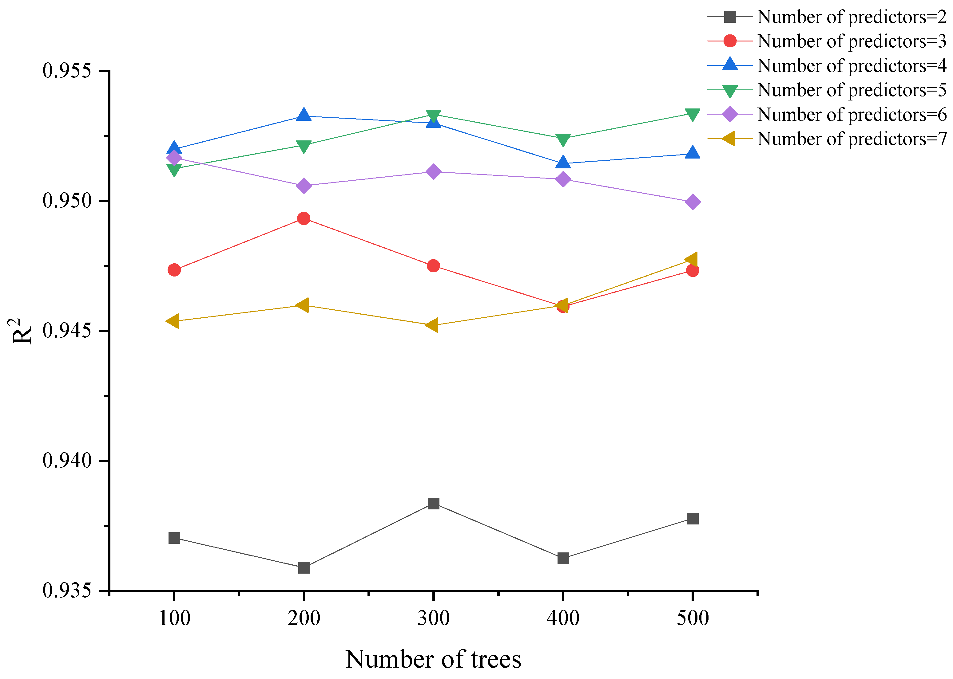
2.4. Tuning RF Hyperparameters Using GridSearchCV

By adjusting the values of its hyperparameters, the RF configuration can be changed [54]. Although the Scikit-learn implementation of the RF default version typically produces satisfactory results without tuning, performance can frequently be improved by hyperparameter adjustment depending on the given features and size of the data [55]. Furthermore, different hyperparameters can be used to control the amount of time spent in learning, the number, and complexity of the decision trees, etc.

The number of decision trees in the forest $\left(B\right)$, as well as the number of features taken into account for each split at each decision tree node ($m$) are the two key factors when utilizing the RF model, as referred previously. $B$ has a default value of 500. A more stable outcome can be achieved by changing the value of $B$ [56]. From the total number of features, one-third of it is considered the default value for $m$ [46]. To obtain the ideal values for the parameters to predict the UCS, a grid search is employed since the performance of RF can be sensitive to $B$ and $m$ [57]. A built-in Scikit-learn technique called “GridSearchCV” was developed to optimize hyperparameters by performing a comprehensive search through a set of parameter values. R² is the most used statistical metric to evaluate models in regression issues. This study used R² to evaluate the RF predictive performance and goodness of fit together with the RMSE. The GridSearchCV yields the best RF estimator by averaging the R² scores of the test folds that were left out during the training process.

2.5. Performance Metrics

A statistical indicator of how well anonymous data are predicted concerning known data is also R² [58], which ranges from 0 to 1. The closer to 1 this metric is, the more accurate the forecast. The following equation is used to compute R².

$${\mathrm{R}}^2=1-\frac{{{\displaystyle \sum }}_{i=1}^n{\left(y_i^{obs}-y_l^{pre}\right)}^2}{{{\displaystyle \sum }}_{i=1}^n{\left(y_i^{obs}-y_i^{-obs}\right)}^2}$$

(1)

where $y_i^{-obs}$ is the mean of the actual data, $n$ denotes the number of observations, and $y_i^{pre}$ and $y_i^{obs}$ denote the ith observation of the actual data and forecasted data, respectively.

The variance of the residuals is the square root of the RMSE. It displays the model’s overall fit to the data or how well the observed data points match the values the model predicts. If the model’s primary goal is prediction, this is the most crucial fit criteria.

$$\mathrm{RMSE}=\sqrt{\frac{1}{n}{{\displaystyle \sum }}_{i=1}^n{\left(y_i^{obs}-y_l^{pre}\right)}^2}$$

(2)

The mean absolute error (MAE) can be computed from the following equation:

$$\mathrm{MAE} = \frac{{{\displaystyle \sum }}_{i=1}^n\left|y_i^{obs}-y_i^{pre}\right|}{n}$$

(3)

3. Database Used

The current investigation used a database with 283 UCS test results [59]. The data was obtained by analyzing three different clayey soil types at three identified locations in Silchar, India, with 2 m below the earth’s surface. According to the Unified Soil Classification System (USCS), the classification of soils is CH, CH, and CL, with the optimal moistures being 19.05, 19.26, and 23.89; liquid limits being 37.68%, 82.15%, and 116.27%; plastic limits being 23.61%, 25.69%, and 27.81%; and plasticity index being 14.07%, 56.46%, and 88.46%, respectively. The CH soil represents inorganic clays of high plasticity and fat clays, while CL represents Inorganic clays of low to medium plasticity, gravelly clays, sandy clays, silty clays, and lean clays. The clayey soil dry was mixed with 50, 40, 35, 30, 25, 20, 16, 12, 8, and 4 percent in weight of ground-granulated blast-furnace slag (%S) as a binder. The soil was also mixed with 20, 16, 12, 8, 4, and 0 percent of fly ash (FA%) also as a binder. In addition, alkali-to-binder ratios (A/B) with values of 0.85, 0.65, and 0.45 were also investigated, along with six molar concentrations of an alkali solution (M) with the following values: 15, 14.5, 12, 10, 8, and 4. Mozumder and Laskar (2015) [59] provided comprehensive information on the chemical and physical features of the sources. The samples that were prepared in molds were maintained in the lab for 24 h before being continuously cured in water for 28 days. After curing, samples were allowed to air dry for an hour at room temperature before testing. The final database included PI, S%, FA%, M, A/B, Na/Al, and Si/Al as the inputs and UCS as the output.

Table 1. Model variable descriptive statistics.

Statistics	(PI) (%)	S (%)	FA(%)	(M) (mol/L)	(A/B)	(Na/Al)	(Si/Al)	UCS (MPa)
Standard deviation	30.73	12.92	4.66	2.73	0.14	0.44	0.35	6.49
Mean	38.83	15.90	2.12	12.42	0.62	1.17	1.70	5.77
Median	14.07	16.00	0.00	12.00	0.65	1.18	1.49	2.91
Maximum	88.46	50.00	20.00	15.00	0.85	1.98	2.49	24.26
Minimum	14.07	0.00	0.00	4.00	0.45	0.24	1.49	0.00
Kurtosis	−1.28	0.30	4.97	2.57	−1.03	−0.62	0.36	−0.47

summarizes the statistical features of the available experimental data.

4. Model Result

4.1. Hyperparameter Optimization: GridSearchCV

It was feasible to identify the parameters that matched the predicted model characteristics by using the GridSearchCV method’s exhaustive parameter search. This method makes it simpler to locate parameters that have the best model estimate accuracy [60]. By specifying the hyperparameter’s values and ranges and using the GridSearchCV function, the optimal set of RF hyperparameters was discovered. Figure 3 displays the outcomes of the GridSearchCV. The 500-tree forest with five predictors produces the maximum R². The models started to overfit when there were more than five predictors. More predictors in a model tend to increase the risk of overfitting the data due to the curse of dimensionality. Additionally, a simpler model lowers the cost of computation. Consequently, 500 trees and five predictors were used to create the final RF model.

4.2. Evaluation of RF Model

Figure 4 compares the measured and estimated UCS values for both the training and testing sets. From Figure 4, it can be seen that the equality line (red line) is surrounded by most of the data points. The RF model has RMSE = 0.4823 and R² = 0.9949 in the training group. However, the performance of the test set is slightly lower than the one of the training set, with RMSE = 0.9815 and R² = 09757. A lower R² generally indicates overfitting in the testing set. However, this is not a significant issue for the RF model study, given the high R² and low RMSE values that were attained. The RF method uses several regression trees and sets of input variables at random to uncover internal relationships between features. The randomness significantly enhances the resilience of the model. Because it splits at nodes, the RF model’s regression trees can be considered an ensemble approach. Then, the RF model combines such functions to avoid having a lot of variation in a single tree.

4.3. Comparison between RF with Linear Regression

The predicted UCS values using a linear regression technique are shown against the relevant observations in Figure 5. A regularized version of the linear regression approach, known as Ridge Regression, was used to manage any possible overfitting problems in the linear regression. The Ridge Regression applies a penalty to reduce the size of the regression coefficients [49]. This penalty is accomplished through a sum of squares penalty-minimized residual. A thorough definition of ridge regression can be found in [49], which also provides examples of how the penalized coefficients frequently reduce variance and lessen overfitting.

The R² values from the ridge regression model for both the testing and training sets are 0.7121 and 0.8379, respectively, as shown in Figure 5. A lower R² value indicates underfitting and suggests that the model cannot adequately account for data variance [49]. In comparison to the RF, the ridge regression performed significantly poorer. This is most likely due to the linear regression model’s inability to handle the UCS and variable nonlinearity.

4.4. Comparison between RF with Previously Developed Models

In this study, to emphasize the prediction power of the RF model, the results from the model are compared to those of the most recently developed white-box ML models. Three white-box ML models were considered: multivariable regression model (MLSR) [34], multi-gen genetic programming (MGGP) [34], and multivariable regression (MVR) [59]. The goal of MGGP is to produce “multi-gene” mathematical models of predictor response data, which are composed of low-order nonlinear combinations of the input variables [61]. On the other side, MLSR and MVR were based on the conventional linear regression method. The accuracy of the models stated above was evaluated using their Mean Absolute Error (MAE). In Figure 6, the MAE values for all previously produced models and for the RF model are presented to demonstrate the model’s correctness. The proposed model in this study has the lowest MAE, as demonstrated. Furthermore, among pre-existing white-box ML models, the MGGP [34] correlation model is the most accurate, while the MLSR [34] correlation model is the poorest.

Table 2. RF and previously developed white-box machine learning models measures performances.

Model	RMSE (MPa)	R2	MAE (MPa)
RF	0.616	0.985	0.351
MGGP [34]	1.790	0.924	1.354
MLSR [34]	3.739	0.788	2.656
MVR [59]	2.777	0.817	2.220

summarizes other statistical quality indicators for the pre-existing models and the RF model for the whole dataset prediction. From Table 2, the RF model in this study has the lowest MAE and RMSE, as well as the maximum R², demonstrating that it is the most efficient and robust model. Figure 7 displays the absolute error for the UCS prediction versus the cumulative frequency of the proposed and pre-existing models. The proposed model (RF) predicts the UCS of 70% of the data with an absolute error of fewer than 0.4 MPa and 80% with an absolute error of fewer than 0.57 MPa. On the other hand, the proposed model in this study predicted only 10% of the experimental data with an absolute error higher than 0.93 MPa. The model from Soleimani et al. [34] (MGGP eq.), which was the second most precise model, correctly predicted 14% of the experimental data and 21% of the UCS measurements with absolute relative errors lower than 0.4 MPa and 0.57 MPa, respectively.

5. SHAP Analysis

Lundberg and Lee [62] proposed SHAP analysis, a unified method for understanding ML models, which incorporates the idea of Shapely Additive explanations as an alternative to other sensitivity analyses. The Shapely value can be visualized as the relative importance and contribution of a given variable to produce the final output variable. The idea is comparable to a parametric study, in which all other variables are held fixed while a single variable is changed to study how that variable affects the target feature. Here, the effect of the input variables on the UCS is defined by discussing the relative weights of several factors to calculate the UCS values.

The summary plot is shown in Figure 8, which illustrates the trend of the corresponding variable and the distribution of SHAP values for each characteristic. The specific SHAP value is shown on the x-axis of the summary plot, while the input variables that were employed in this research are ordered according to their importance along the y-axis. Depending on which side the red dots are on, the red instances signify higher values with an impact on the model prediction. SHAP values for each variable are shown against the change in their respective inputs on the horizontal x-axis, illustrating the degree to which each variable can be predicted (blue to red). It is clear that ground-granulated blast-furnace slag (%S), plasticity index (PI), the ratios of sodium to aluminum, and the molar concentrations of an alkali solution (M) all considerably contribute to the UCS prediction. The amount of fly ash percentage (FA%), the alkali-to-binder ratio (A/B), and the silicon-to-aluminum ratio (Si/Al) are less relevant. The improvement in UCS that results from an increase in S is seen in Figure 8. This was to be expected since a larger content of S is a sign of a higher quantity of binder being present in the mixture and, thus, a higher UCS. The findings obtained from this analysis are in high accordance with the ones published by several other researchers [34,59,63]. According to the findings of the SHAP study, a higher PI leads to a lower UCS, as observed in Figure 8. This result was also expected. If the PI increases, the proportion of polymer emulsion to the bentonite content, which normally stays together, will change. In addition, research has shown that raising the PI reduces the stiffness and peak strength of the soil while also making it more ductile [34,64]. As shown in Figure 8, increasing both M and A/B improves the UCS of the geopolymer-stabilized clayey soil. This result is not a surprise, given that the concentration of alkali (NaOH) is one of the most important parameters in geopolymerization [37]. A higher concentration of NaOH enhances the UCS while simultaneously reducing the mix workability. This is caused by an increase in the solubility of aluminosilicate [34,65,66,67].

Figure 8 also illustrates the results of analyzing the effects of the Si/Al and Na/Al combinations. UCS is governed by the kinetic reactions during the synthetization of the geopolymer, which is controlled by the interaction of these factors. According to previous research [59,68], an increase in the ratios of Si/Al and Na/Al causes an increase in the UCS.

Streamlit (https://streamlit.io) was used to develop an interactive web application using the improved ML model based on the RF algorithms. It enables quick predictions of the UCS by the ML model using the inputs PI, S%, FA%, M, A/B, Na/Al, and Si/Al. The ranges of the input variables that can be chosen match those that were used to train the model (see “Database Used” section). The web application can be accessed at [69]. It has been deployed to the cloud. Any web browser, even mobile ones, can be used to open and execute it.

6. Conclusions

This work used rigorous machine learning approaches based on a robust algorithm named Random Forest (RF) to simulate unconfined compressive strength (UCS) in clayey soil stabilized with geopolymer. The performance of the predictions was enhanced by tuning the hyperparameters of the investigated RF schemes using a GridSearchCV-based approach:

• The suggested RF model showed a high coefficient of determination of 0.9757 on the test set, indicating that it is highly accurate in forecasting. Additionally, no overfitting was generated, as concluded by the extremely low RMSE values on the training and testing sets.
• The generated model capacity to predict outcomes was contrasted with the one generated by previously proposed models in [34] and [59], which were: multivariable regression model (MLSR), multi-gen genetic programming (MGGP), and multivariable regression (MVR). According to the statistical analysis, the suggested RF model outperformed the current white-box models regarding relative errors and determination coefficients.
• Shap analysis was used to demonstrate the implemented RF’s strong integrity and reliability.

This study can be expanded to predict other soil properties, such as those found with standard penetration tests (SPT), compaction testing, or triaxial tests. Moreover, the generalization capacity of the RF model could be further enhanced if a larger dataset with more affecting factors can be acquired in the future. Therefore, future studies will concentrate on developing a larger dataset and considering more factors, such as time duration and admixture types.

Finally, to popularize and apply the proposed model for practice, a web application (app) using this model was developed to help civil engineers to predict the UCS for projects [69]. This app can constitute a valuable tool, complementary or even alternative to experimental testing procedures, saving costs, time, and human resources.

References

1. Hussain, A.; Al-Khafaji, Z. Reduction of environmental pollution and improving the (Mechanical, physical and chemical characteristics) of contaminated clay soil by using of recycled oil. J. Adv. Res. Dyn. Control Syst. 2020, 12, 1276–1286. [Google Scholar] [CrossRef]
2. Al-Khafaji, Z.; Al-Naely, H.; Al-Najar, A. A review applying industrial waste materials in stabilisation of soft soil. Electron. J. Struct. Eng. 2018, 18, 16–23. [Google Scholar] [CrossRef]
3. Vukićević, M.; Marjanović, M.; Pujević, V.; Jocković, S. The alternatives to traditional materials for subsoil stabilization and embankments. Materials 2019, 12, 3018. [Google Scholar] [CrossRef] [PubMed] [Green Version]
4. Tiwari, N.; Satyam, N. Experimental study on the influence of polypropylene fiber on the swelling pressure expansion attributes of silica fume stabilized clayey soil. Geosciences 2019, 9, 377. [Google Scholar] [CrossRef] [Green Version]
5. Shen, J.; Xu, Y.; Chen, J.; Wang, Y. Study on the stabilization of a new type of waste solidifying agent for soft soil. Materials 2019, 12, 826. [Google Scholar] [CrossRef] [Green Version]
6. She, J.; Lu, Z.; Yao, H.; Fang, R.; Xian, S. Experimental study on the swelling behavior of expansive soil at different depths under unidirectional seepage. Appl. Sci. 2019, 9, 1233. [Google Scholar] [CrossRef] [Green Version]
7. Suksiripattanapong, C.; Sakdinakorn, R.; Tiyasangthong, S.; Wonglakorn, N.; Phetchuay, C.; Tabyang, W. Properties of soft Bangkok clay stabilized with cement and fly ash geopolymer for deep mixing application. Case Stud. Constr. Mater. 2022, 16, e01081. [Google Scholar] [CrossRef]
8. Parthiban, D.; Vijayan, D.S.; Koda, E.; Vaverkova, M.D.; Piechowicz, K.; Osinski, P.; Van, D.B. Role of Industrial based Precursors in the Stabilization of weak soils with geopolymer-A Review. Case Stud. Constr. Mater. 2022, 16, e00886. [Google Scholar] [CrossRef]
9. Murmu, A.L.; Dhole, N.; Patel, A. Stabilisation of black cotton soil for subgrade application using fly ash geopolymer. Road Mater. Pavement Des. 2020, 21, 867–885. [Google Scholar] [CrossRef]
10. Khasib, I.A.; Daud, N.N.N. Physical and Mechanical Study of Palm Oil Fuel Ash (POFA) based Geopolymer as a Stabilizer for Soft Soil. Pertanika J. Sci. Technol. 2020, 28, 149–160. [Google Scholar] [CrossRef]
11. Ghadir, P.; Zamanian, M.; Mahbubi-Motlagh, N.; Saberian, M.; Li, J.; Ranjbar, N. Shear strength and life cycle assessment of volcanic ash-based geopolymer and cement stabilized soil: A comparative study. Transp. Geotech. 2021, 31, 100639. [Google Scholar] [CrossRef]
12. Ramesh, T.; Prakash, R.; Shukla, K. Life cycle energy analysis of buildings: An overview. Energy Build. 2010, 42, 1592–1600. [Google Scholar] [CrossRef]
13. Fakhrabadi, A.; Ghadakpour, M.; Choobbasti, A.J.; Kutanaei, S.S. Evaluating the durability, microstructure and mechanical properties of a clayey-sandy soil stabilized with copper slag-based geopolymer against wetting-drying cycles. Bull. Eng. Geol. Environ. 2021, 80, 5031–5051. [Google Scholar] [CrossRef]
14. Al-Dossary, A.A.; Awed, A.M.; Gabr, A.R.; Fattah, M.Y.; El-Badawy, S.M. Performance enhancement of road base material using calcium carbide residue and sulfonic acid dilution as a geopolymer stabilizer. Constr. Build. Mater. 2023, 364, 129959. [Google Scholar] [CrossRef]
15. Salas, D.A.; Ramirez, A.D.; Ulloa, N.; Baykara, H.; Boero, A.J. Life cycle assessment of geopolymer concrete. Constr. Build. Mater. 2018, 190, 170–177. [Google Scholar] [CrossRef]
16. Shekhawat, P.; Sharma, G.; Singh, R.M. A Comprehensive Review of Development and Properties of Flyash-Based Geopolymer as a Sustainable Construction Material. Geotech. Geol. Eng. 2022, 40, 5607–5629. [Google Scholar] [CrossRef]
17. Shekhawat, P.; Sharma, G.; Singh, R.M. Microstructural and morphological development of eggshell powder and flyash-based geopolymers. Constr. Build. Mater. 2020, 260, 119886. [Google Scholar] [CrossRef]
18. de Araújo, M.T.; Ferrazzo, S.T.; Chaves, H.M.; da Rocha, C.G.; Consoli, N.C. Mechanical behavior, mineralogy, and microstructure of alkali-activated wastes-based binder for a clayey soil stabilization. Constr. Build. Mater. 2023, 362, 129757. [Google Scholar] [CrossRef]
19. Turner, L.K.; Collins, F.G. Carbon dioxide equivalent (CO2-e) emissions: A comparison between geopolymer and OPC cement concrete. Constr. Build. Mater. 2013, 43, 125–130. [Google Scholar] [CrossRef]
20. Abdila, S.R.; Abdullah, M.M.A.B.; Ahmad, R.; Nergis, B.; Doru, D.; Rahim, S.Z.A.; Omar, M.F.; Sandu, A.V.; Vizureanu, P. Potential of soil stabilization using ground granulated blast furnace slag (GGBFS) and fly ash via geopolymerization method: A Review. Materials 2022, 15, 375. [Google Scholar] [CrossRef]
21. Khademi, F.; Budiman, J. Expansive soil: Causes and treatments. i-Manag. J. Civ. Eng. 2016, 6, 1. [Google Scholar]
22. Long, Z.; Cheng, Y.; Yang, G.; Yang, D.; Xu, Y. Study on triaxial creep test and constitutive model of compacted red clay. Int. J. Civ. Eng. 2021, 19, 517–531. [Google Scholar] [CrossRef]
23. Emarah, D.A.; Seleem, S.A. Swelling soils treatment using lime and sea water for roads construction. Alex. Eng. J. 2018, 57, 2357–2365. [Google Scholar] [CrossRef]
24. Di Sante, M.; Di Buò, B.; Fratalocchi, E.; Länsivaara, T. Lime treatment of a soft sensitive clay: A sustainable reuse option. Geosciences 2020, 10, 182. [Google Scholar] [CrossRef]
25. Salimi, M.; Ghorbani, A. Mechanical and compressibility characteristics of a soft clay stabilized by slag-based mixtures and geopolymers. Appl. Clay Sci. 2020, 184, 105390. [Google Scholar] [CrossRef]
26. Phummiphan, I.; Horpibulsuk, S.; Rachan, R.; Arulrajah, A.; Shen, S.-L.; Chindaprasirt, P. High calcium fly ash geopolymer stabilized lateritic soil and granulated blast furnace slag blends as a pavement base material. J. Hazard. Mater. 2018, 341, 257–267. [Google Scholar] [CrossRef]
27. Martins, A.C.P.; de Carvalho, J.M.F.; Costa, L.C.B.; Andrade, H.D.; de Melo, T.V.; Ribeiro, J.C.L.; Pedroti, L.G.; Peixoto, R.A.F. Steel slags in cement-based composites: An ultimate review on characterization, applications and performance. Constr. Build. Mater. 2021, 291, 123265. [Google Scholar] [CrossRef]
28. Sharma, A.K.; Sivapullaiah, P. Ground granulated blast furnace slag amended fly ash as an expansive soil stabilizer. Soils Found. 2016, 56, 205–212. [Google Scholar] [CrossRef]
29. Alam, S.; Das, S.K.; Rao, B.H. Strength and durability characteristic of alkali activated GGBS stabilized red mud as geo-material. Constr. Build. Mater. 2019, 211, 932–942. [Google Scholar] [CrossRef]
30. Motamedi, S.; Song, K.-I.; Hashim, R. Prediction of unconfined compressive strength of pulverized fuel ash–cement–sand mixture. Mater. Struct. 2015, 48, 1061–1073. [Google Scholar] [CrossRef]
31. Gunaydin, O.; Gokoglu, A.; Fener, M. Prediction of artificial soil’s unconfined compression strength test using statistical analyses and artificial neural networks. Adv. Eng. Softw. 2010, 41, 1115–1123. [Google Scholar] [CrossRef]
32. Abbey, S.; Ngambi, S.; Ganjian, E. Development of strength models for prediction of unconfined compressive strength of cement/byproduct material improved soils. Geotech. Test. J. 2017, 40, 928–935. [Google Scholar] [CrossRef]
33. Suthar, M. Applying several machine learning approaches for prediction of unconfined compressive strength of stabilized pond ashes. Neural Comput. Appl. 2020, 32, 9019–9028. [Google Scholar] [CrossRef]
34. Soleimani, S.; Rajaei, S.; Jiao, P.; Sabz, A.; Soheilinia, S. New prediction models for unconfined compressive strength of geopolymer stabilized soil using multi-gen genetic programming. Measurement 2018, 113, 99–107. [Google Scholar] [CrossRef]
35. Mozumder, R.A.; Laskar, A.I.; Hussain, M. Empirical approach for strength prediction of geopolymer stabilized clayey soil using support vector machines. Constr. Build. Mater. 2017, 132, 412–424. [Google Scholar] [CrossRef]
36. Chemmakh, A. Machine Learning Predictive Models to Estimate the UCS and Tensile Strength of Rocks in Bakken Field. In Proceedings of the SPE Annual Technical Conference and Exhibition, Dubai, United Arab Emirates, 21–23 September 2021. [Google Scholar]
37. Nagaraju, T.V.; Prasad, C. New prediction models for compressive strength of GGBS-based geopolymer clays using swarm assisted optimization. In Advances in Computer Methods and Geomechanics; Springer: Singapore, 2020; pp. 367–379. [Google Scholar]
38. Gullu, H. On the prediction of unconfined compressive strength of silty soil stabilized with bottom ash, jute and steel fibers via artificial intelligence. Geomech. Eng. 2017, 12, 441–464. [Google Scholar] [CrossRef]
39. Sun, Y.; Li, G.; Zhang, J. Developing hybrid machine learning models for estimating the unconfined compressive strength of jet grouting composite: A comparative study. Appl. Sci. 2020, 10, 1612. [Google Scholar] [CrossRef]
40. Zhang, W.; Li, H.; Li, Y.; Liu, H.; Chen, Y.; Ding, X. Application of deep learning algorithms in geotechnical engineering: A short critical review. Artif. Intell. Rev. 2021, 54, 5633–5673. [Google Scholar] [CrossRef]
41. Pham, B.T.; Hoang, T.-A.; Nguyen, D.-M.; Bui, D.T. Prediction of shear strength of soft soil using machine learning methods. Catena 2018, 166, 181–191. [Google Scholar] [CrossRef]
42. Majidifard, H.; Jahangiri, B.; Buttlar, W.G.; Alavi, A.H. New machine learning-based prediction models for fracture energy of asphalt mixtures. Measurement 2019, 135, 438–451. [Google Scholar] [CrossRef]
43. Kardani, N.; Zhou, A.; Nazem, M.; Shen, S.-L. Estimation of bearing capacity of piles in cohesionless soil using optimised machine learning approaches. Geotech. Geol. Eng. 2020, 38, 2271–2291. [Google Scholar] [CrossRef]
44. Bui, D.T.; Nhu, V.-H.; Hoang, N.-D. Prediction of soil compression coefficient for urban housing project using novel integration machine learning approach of swarm intelligence and multi-layer perceptron neural network. Adv. Eng. Inform. 2018, 38, 593–604. [Google Scholar]
45. Chen, X.; Ishwaran, H. Random forests for genomic data analysis. Genomics 2012, 99, 323–329. [Google Scholar] [CrossRef] [PubMed] [Green Version]
46. Breiman, L. Random forests. Mach. Learn. 2001, 45, 5–32. [Google Scholar] [CrossRef] [Green Version]
47. Mitchell, T.M.; Mitchell, T.M. Machine Learning; McGraw-Hill New York: New York, NY, USA, 1997; Volume 1. [Google Scholar]
48. Breiman, L.; Friedman, J.H.; Olshen, R.A.; Stone, C.J. Classification and Regression Trees; Routledge: London, UK, 2017. [Google Scholar]
49. Hastie, T.; Tibshirani, R.; Friedman, J. The Elements of Statistical Learning; Springer Series in Statistics; Springer: New York, NY, USA, 2001. [Google Scholar]
50. Gong, H.; Sun, Y.; Shu, X.; Huang, B. Use of random forests regression for predicting IRI of asphalt pavements. Constr. Build. Mater. 2018, 189, 890–897. [Google Scholar] [CrossRef]
51. Tang, L.; Na, S. Comparison of machine learning methods for ground settlement prediction with different tunneling datasets. J. Rock Mech. Geotech. Eng. 2021, 13, 1274–1289. [Google Scholar] [CrossRef]
52. Hastie, T.; Tibshirani, R.; Friedman, J.H. The Elements of Statistical Learning: Data Mining, Inference, and Prediction; Springer: New York, NY, USA, 2009; Volume 2. [Google Scholar]
53. Liaw, A.; Wiener, M. Classification and regression by randomForest. R News 2002, 2, 18–22. [Google Scholar]
54. Probst, P.; Wright, M.N.; Boulesteix, A.L. Hyperparameters and tuning strategies for random forest. Wiley Interdiscip. Rev. Data Min. Knowl. Discov. 2019, 9, e1301. [Google Scholar] [CrossRef] [Green Version]
55. Scornet, E. Tuning parameters in random forests. Esaim Proc. Surv. 2017, 60, 144–162. [Google Scholar] [CrossRef] [Green Version]
56. Kuhn, M.; Johnson, K. Applied Predictive Modeling; Springer: New York, NY, USA, 2013; Volume 26. [Google Scholar]
57. Grimm, R.; Behrens, T.; Märker, M.; Elsenbeer, H. Soil organic carbon concentrations and stocks on Barro Colorado Island—Digital soil mapping using Random Forests analysis. Geoderma 2008, 146, 102–113. [Google Scholar] [CrossRef]
58. Rashed, K.A.; Salih, N.B.; Abdalla, T.A. Prediction of California Bearing Ratio from Consistency and Compaction Characteristics of Fine-grained Soils. Al-Nahrain J. Eng. Sci. 2021, 24, 123–129. [Google Scholar] [CrossRef]
59. Mozumder, R.A.; Laskar, A.I. Prediction of unconfined compressive strength of geopolymer stabilized clayey soil using artificial neural network. Comput. Geotech. 2015, 69, 291–300. [Google Scholar] [CrossRef]
60. Lu, J.; Zhang, Y.; Chen, M.; Wang, L.; Zhao, S.; Pu, X.; Chen, X. Estimation of monthly 1 km resolution PM2. 5 concentrations using a random forest model over “2 + 26” cities, China. Urban Clim. 2021, 35, 100734. [Google Scholar] [CrossRef]
61. Gandomi, A.H.; Alavi, A.H. A new multi-gene genetic programming approach to nonlinear system modeling. Part I: Materials and structural engineering problems. Neural Comput. Appl. 2012, 21, 171–187. [Google Scholar] [CrossRef]
62. Lundberg, S.M.; Lee, S.-I. A unified approach to interpreting model predictions. In Proceedings of the 31st Conference on Neural Information Processing Systems (NIPS 2017), Long Beach, CA, USA, 4–9 December 2017; pp. 4768–4777. [Google Scholar]
63. Singhi, B.; Laskar, A.I.; Ahmed, M.A. Investigation on soil–geopolymer with slag, fly ash and their blending. Arab. J. Sci. Eng. 2016, 41, 393–400. [Google Scholar] [CrossRef]
64. Naeini, S.A.; Naderinia, B.; Izadi, E. Unconfined compressive strength of clayey soils stabilized with waterborne polymer. Ksce J. Civ. Eng. 2012, 16, 943–949. [Google Scholar] [CrossRef]
65. Somna, K.; Jaturapitakkul, C.; Kajitvichyanukul, P.; Chindaprasirt, P. NaOH-activated ground fly ash geopolymer cured at ambient temperature. Fuel 2011, 90, 2118–2124. [Google Scholar] [CrossRef]
66. Sathonsaowaphak, A.; Chindaprasirt, P.; Pimraksa, K. Workability and strength of lignite bottom ash geopolymer mortar. J. Hazard. Mater. 2009, 168, 44–50. [Google Scholar] [CrossRef]
67. Khale, D.; Chaudhary, R. Mechanism of geopolymerization and factors influencing its development: A review. J. Mater. Sci. 2007, 42, 729–746. [Google Scholar] [CrossRef]
68. Duxson, P.; Fernández-Jiménez, A.; Provis, J.L.; Lukey, G.C.; Palomo, A.; van Deventer, J.S. Geopolymer technology: The current state of the art. J. Mater. Sci. 2007, 42, 2917–2933. [Google Scholar] [CrossRef]
69. Available online: https://hamza19901990-soil-streamlit-soil-wnlfpg.streamlit.app/ (accessed on 5 January 2023).
Figure 1. Research Methodology.
Sustainability 15 01408 g001
Figure 2. The RF prediction algorithm.
Sustainability 15 01408 g002
Figure 3. Results from the hyperparameter tuning by using five-fold cross-validation.
Sustainability 15 01408 g003
Figure 4. Predicted UCS by RF.
Sustainability 15 01408 g004
Figure 5. Predicted UCS by Ridge Regression Model.
Sustainability 15 01408 g005
Figure 6. Comparison between the performances of the RF and prior models.
Sustainability 15 01408 g006
Figure 7. Cumulative frequency vs. absolute residual for the RF model and the prior white-box ML models (Soleimani et al. [34], Mozumder and Laskar [59]).
Sustainability 15 01408 g007
Figure 8. Summary plot of SHAP values.
Sustainability 15 01408 g008