A National and Regional Greenhouse Gas Breakeven Assessment of EVs across North America

Abstract

Electrification is considered key to decarbonizing the transport sector. While electric vehicles (EVs) lack tailpipe emissions, battery and electricity production can lead to significant emissions. This study analysed whether EVs can effectively mitigate GHG emissions in North America, by calculating two GHG breakeven indicators for EVs and comparing them to internal combustion engine vehicles (ICEVs). EV life cycle emissions were compared to those of ICEVs in Canada, Mexico, and the USA. In addition, this study considered potential national electricity grids evolutions and improvements in battery production and vehicle efficiency. The study estimated that EVs in Canada, the USA, and Mexico would see environmental benefits after 18.0, 25.1, and 25.6 thousand driven kilometres, respectively, as compared to petrol vehicles. Regionally, Québec had the lowest emissions (12.9 tCO₂eq) for EVs while Iowa (62.0) had the highest. In several states, EVs did not outperform ICEVs. Emissions from EVs are expected to decrease in coming years as the carbon intensity of electrical grids decreases. Policies should consider prioritising grid decarbonization over EV uptake where regional grid GHG intensity is high. This work provides one of the first regional and international case studies determining the environmental breakeven points of EVs when considering trade.

1. Introduction

Greenhouse gas (GHG) emissions, along with other anthropogenic impacts on the planet, have grown exponentially in stride with socio-economic trends such as population, GDP, and transportation, leading to suggestions that humanity has entered a new geological era, the Anthropocene [1].

In 2015, the Paris Agreement was signed with the goal of keeping global temperatures from reaching 2 °C above pre-industrial levels, ideally below 1.5 °C. This agreement was hailed as a landmark for climate action, with most countries around the world setting Nationally Declared Contributions (NDCs) for reductions in greenhouse gas (GHG) emissions; however, the IPCC believes that the achievement of this goal is peril. The IPCC has estimated that there is a 40% chance that by 2025 the yearly average temperature will already have surpassed the 1.5 °C pre-industrial level threshold, and five years after the adoption of the Paris Agreement the emissions gap is as wide as ever [2].

North America is the region with the second largest GHG emissions in the world, behind East Asia [3], and needs to take significant action to reduce emissions. In terms of per capita emissions, Canada and the USA both emit 14.2 tonnes CO₂eq per capita. Mexico, on the other hand, emits only 2.8 tonnes per capita, and as such is the only country in this study with emissions below the global average of 4.8 tonnes [4]. However, Mexico falls behind in terms of development indicators, and this lack of social provisioning is related to its lower CO₂ emissions [5].

Emissions from transport account for 14% of global anthropogenic GHG emissions and one quarter of global CO₂ emissions, and are set to be the fastest growing source of emissions, growing at a rate of approximately 2% per year. 72% of these emissions come from road transport [3,6]. The transport sector has a higher impact in North America than in any other region [2,3,7]. Considering the climate, energy security, and fossil fuel supply/price volatility, high hopes are being placed on electrification of the transport sector, particularly the private vehicle fleet [8,9].

In Canada, transportation accounted for 30% of the country’s emissions in 2020 [10]. The country has implemented policies at the national level to encourage adoption of zero-emission vehicles (ZEVs). For example, by 2035 all new light-duty vehicles and passenger trucks must be ZEVs. Canada is additionally investing CAD 150 million in charging and refuelling infrastructure as well as over CAD 300 million in financial incentives [11]. In Canada as a whole, battery electric vehicles (BEVs) and plug-in hybrid electric vehicles (PHEVs) represented a 3.5% share of vehicle sales; however, Québec and British Columbia had 6.8 and 8.4% share, while the rest of Canada had only a 1.3% share [12,13]. Provincial variation is significant in Canada, with transport emissions accounting for up to 43.3% of total emissions in Québec [14].

Transportation represented 29% of U.S. emissions in 2019 [15], with 82% of that coming from road transport [16]. Enormous diversity in transport as a share of emissions exists at the state level, from 12% in Wyoming to 59% in California, Hawaii, and Washington [17]. The USA is one of the largest EV markets, along with China and Europe; together, they account for over 93% of sales [18]. The overall market share is low, however, although the market surged in 2021, jumping from 2 to 4.5% of sales [19]. There is significant disparity between different states. In California, BEV and PHEV sales represented 7.4% of the market in 2019. Meanwhile, in five other states this figure was only 0.3% [20]. Fiscal incentives for people to obtain ZEVs and significant investment in charging infrastructure exist across the country, with a target for 50% of vehicles sold to be electric by 2030 [21]. This should only increase with the newly implemented Inflation Reduction Act (IRA), which places a significant focus on reducing GHG from transportation through subsidies for electric vehicles and grid decarbonisation [22].

In Mexico, transportation represents 25% of all the emissions from the country [23]. The government is working towards increasing electromobility, with financial incentives available for EVs and PHEVs. These include tax exemption for EV imports, exports, purchases, as well as exemption from certain road tolls [24]. Mexico has a pending National Electromobility Strategy, which aims for 29.5% of vehicles sold in 2035 to be electric [25]. In Mexico, EVs and hybrid EVs only accounted for 1.7% of sales in 2020, and the majority of these were non-plug-in hybrids. When accounting only for BEVs and PHEVs, this figure decreases to 0.21% of the market [26].

While EVs are generally considered environmentally friendly alternatives to conventional internal combustion engine vehicles (ICEVs), the production of their batteries requires an enormous amount of energy and can lead to significant of GHG emissions [27]. The battery and vehicle weights have been found to be significant drivers of impact in the manufacturing phase [28]. The potential lifespan of batteries additionally impacts these assumptions [29]. Furthermore, the electricity required to power EVs must have a source, and the emissions of an EV vary greatly depending on whether the electricity comes from solar, nuclear, or coal power [30]. Ambient weather conditions further influence the efficiency of EVs (e.g., [31,32,33], yet have rarely been incorporated into national and regional environmental breakeven studies (e.g., [34,35,36]).

Previous studies have shown that while EVs typically outperform ICEVs in terms of life cycle GHGs [37,38], in highly GHG intensive grid conditions this is not necessarily always the case [39]. Moreover, in many locations the distance intersection point (DIP), the point at which an EV with typically higher production phase emissions becomes a lower emission alternative to an ICEV, is passed only late in the lifetime of a vehicle [36,39]. In [40], the need to take temporal perspectives into account when performing EV LCA studies is further recognized, as varying rates of decarbonization have a significant impact on final outcomes.

To fill these gaps, the present study focuses on the three North American countries of Mexico, the USA, and Canada, and addresses the following research questions:

• How does the GHG intensity of electrical grids across North America affect the life cycle emissions, DIP and ED of EVs in comparison to ICEVs?
• How do grid decarbonisation, fuel efficiency improvements, and less GHG-intensive production affect these metrics?

This research makes the following contributions. First, this work performs the first spatial assessment of EV environmental performance across North America that incorporates electricity trading. This approach has been taken in Europe [39]. In [41], the authors performed a spatial LCA of EVs, although their study did not include regional electricity trade and was largely focused on the electrification of heavy-duty vehicles. In [42], the authors performed a comparative carbon footprint analysis in the US; however, they did not include interstate trading and published in 2015, making the data likely outdated considering the rapid development of EVs. Mexico and Canada were not included in their study, making cross-country comparisons difficult, particularly with respect to the varying decarbonization commitments made by each country, as shown in [43]. The inclusion of Mexico addresses the call in [44] for increased representation of developing country case studies.

Second, the present work shows the influence of current decarbonization strategies on the mitigation potential of EVs in each national context, addressing the research gap identified by [40]. Further, this work is one of few studies which performs both national and regional assessments in the same study, which for the first time allows for a consistent mental bridging of these results, illustrating how the many studies (e.g., [34,35,39,43] which discuss national results only provide a general depiction of average performance and that regional results are needed for more targeted interventions. Lastly, this work makes a set of policy recommendations based off these results, which includes the need to establish an EV incentive system which works to maximize the environmental benefits of their introduction, strengthening similar suggestions in the literature [39,41].

To answer the research questions, Section 2 describes the data and methods used to perform these analyses. This study investigated the electricity grids of Canada, Mexico, and the USA currently as well as their future development scenarios in order to estimate the climate performance of EVs against ICEVs. The study examines the sub-national level, looking at all 50 U.S. states, Washington D.C., and Québec. The province of Québec was included as it is a significant producer and exporter of clean renewable energy, with over 99% of its electricity coming from sources with zero direct emissions, notably hydropower (95%) [45]. Section 3 reviews the results of this work, and Section 4 discusses the suitability of the current transportation policies in these countries in terms of GHG emissions in light of the findings.

2. Data and Methods

This section contains a brief overview of the past literature on the subject, then highlights which methods and techniques were taken from these studies, which methods were devised for this study, and how these were combined with data from official government sources to obtain the results in Section 3. It is worth noting that in this study, we only focus on mid-sized electrical vehicles and do not consider fleet-level changes (though this is a worthy avenue of study); we instead focus on the individual performance of single EVs versus single ICEVs.

2.1. Vehicle Production Emissions and EV Efficiency

In this study, the mean emissions from [39] were used for the production emissions shown in

Table 1. The mean emissions and standard deviation of the life cycle phases of EVs and petrol and diesel ICEVs (adapted from [39]).

Vehicle Type	Statistic	Production (tCO2eq)	WTW * (gCO2eq/km)	Maintenance	EOL (gCO2eq/km)
BEV	Mean	10.8	132.2	10.1	0.2
	SD	2.38	107.1	5.06	1.55
Petrol	Mean	6.6	237.1	12.0	0.4
	SD	2.01	63.64	5.55	1.05
Diesel	Mean	6.1	154.3	10.1	−0.6
	SD	1.25	32.7	4.82	1.06

* Note that the WTW emissions in this study are altered according the spatial estimates for the average emission factor incorporating trade.

. While it has been observed before that the inconsistency in the scopes and assumptions of different studies makes it hard to compare them [46], 70% variability in LCA results comes from the GHG intensity of the electricity mix used in the study [30]. Additionally, ambient weather conditions can impact EV efficiencies. Therefore, a second set of results in which these impacts have been added and compared to the results shown below can be found in Appendix B. The energy efficiency estimates under various operating temperatures were extracted from [31,32,33]. Average annual temperatures from [47] were used to estimate spatial efficiencies.

It should be noted that the temperature affects the efficiency of ICEVs as well; these impacts tend to be smaller than for EVs in cold weather, although the reverse is true if the heater is not used [48]. It is possible that motors may become insulated when ICEVs are no longer the dominant vehicle type. Furthermore, higher temperatures can lead to similar inefficiencies and depend heavily on the use of the air conditioner [49]. The more efficient the powertrain, the larger the share of emissions is from heating or cooling the cabin [50]. In light of the enormous dependency of temperature-adjusted results on the drive cycle, temperature has not been accounted for in the primary results. However, temperature-adjusted results are available in Appendix B. A Monte Carlo simulation was performed on these results as a sensitivity analysis, with the results shown in Appendix B. Separate Monte Carlo simulations were then run for each nation/state according to the local conditions using these statistics.

2.2. Grid Electricity Emissions Factors (EF)

A significant issue when looking at EV LCAs is the emissions intensity of the grid, including imports, which can form an important share of consumed electricity [51].

Looking into each country’s grid, in Canada the majority (61%) of electricity produced is from hydropower and other non-emitting sources (21%) [45]. Electricity generation is expected to accelerate over the coming decades, driven by a rapid growth in wind and solar power and a minor increase in hydropower [52]. As for the U.S., 2020 saw renewable electricity sources overtake nuclear and coal, though natural gas continues to represents the greatest share of electricity production. Additionally, in the last decade electricity production appears to have plateaued [53]. Meanwhile in Mexico only 25.4% of electricity came from clean sources in 2020, up from 18.9% in 2019. However, total electricity production from clean sources decreased by 8438 GWh in the same period [54]. Another study found that renewables could be responsible for 76% of Mexico’s electricity by 2050 [55].

In determining the emissions factor associated with these grid compositions, the average electricity mix is suggested as the most practical [56] despite fluctuations depending on the season and time of day. In this study, we use the average production approach including trade.

2.2.1. National EFs

The data on electricity trade between nations was retrieved from [57,58,59] using the following formula, following a similar approach as Moro and Lonza [51]:

$$\mathrm{CEF}=\mathrm{NGEF} \times \frac{\mathrm{G}-\mathrm{Exports}}{\mathrm{C}}+\mathrm{IGEF} \times \frac{\mathrm{Imports}}{\mathrm{C}}$$

(1)

where C represents consumption (in kWh), CEF represents the EF of electricity consumed (in gCO₂eq/kWh), NGEF represents the EF of internally generated electricity (in gCO₂eq/kWh), and IGEF represents the EF of imported electricity (in gCO₂eq/kWh). The generation EFs for Mexico and the USA were available through government agency reports [60,61]. For Canada, total emissions from electricity production and the total electricity produced were used to calculate the EF [10,52].

Table 2. Generation and consumption emissions factors for Canada, Mexico, and the USA.

Country	GEF (gCO2eq/kWh)	CEF (gCO2eq/kWh)
Canada	97	103
Mexico	494	494
USA	482	476

shows the calculated generation and consumption EF for the three nations.

An assumption was made that the imported electricity would have the same average GEF as the nation from which it came. While this may not reflect the exact reality, many states/provinces that exported electricity internationally also imported electricity from other states, meaning that it is impossible to assess exactly where this electricity was from using the information available. Many states had both international imports and exports, which is likely due to grid balancing.

2.2.2. Regional (State) EFs

At the regional level, there was a lack of data available on where interstate electricity trade originated. Information on the GEF for U.S. states was taken from government reports, which provided the total amount of imported and exported electricity per state [61]. This information was used to create an interstate EF using the average EF of traded electricity.

When a state imported internationally and exports nationally, it was assumed that imported electricity was then exported to other states, with the state under study simply acting as a thoroughfare. It is possible that states export nationally when in surplus and import internationally when they have need for additional electricity. However, all of the states which simultaneously import internationally and export locally lie on the USA–Canada border, suggesting that the electricity is merely passing through on their way to other states. This highly uncertain assumption is discussed in Section 4. Further, due to this lack of data availability, this study could not go deeper than the state level, as electricity trading data at a more granular level were not available.

In the EF calculation, exported electricity was subtracted from imported electricity when assessing the share of electricity determined to be consumed in each state. International exports are always assumed to be derived from electricity produced within the state itself, leading to the following equation:

$$\mathrm{EF}=\mathrm{GEF} \times \frac{\mathrm{G}-\mathrm{IntEx}}{\mathrm{C}}+\mathrm{ISEF} \times \frac{\mathrm{NatIm}}{\mathrm{C}}+\mathrm{CMEF} \times \frac{\mathrm{IntIm}-\mathrm{NatEx}}{\mathrm{C}}$$

(2)

In this equation, the GEF (gCO₂eq/kWh) represents the EF of electricity generated within the state, while the CMEF (gCO₂eq/kWh) is the EF of either Canada or Mexico, according to the country the state imports from. The ISEF (gCO₂eq/kWh) represents the interstate emissions factor.

The importance of electricity imports on EF is clear. For example, the EF of Washington D.C. decreased from 1304 to 500 gCO₂eq/kWh when interstate and international trade were taken into account, and that of Idaho increased 50% from 192 to 289 gCO₂eq/kWh.

The final calculations showed huge variation between states, with the EF ranging from 118 gCO₂eq/kWh in Vermont to 1600 gCO₂eq/kWh in Iowa. Meanwhile, in Québec, where 99% of electricity comes from renewable sources, the EF was 0.1 gCO₂eq/kWh. A full list of regional EFs can be found in Appendix A.

2.3. Environmental Performance Indicators (EPI)

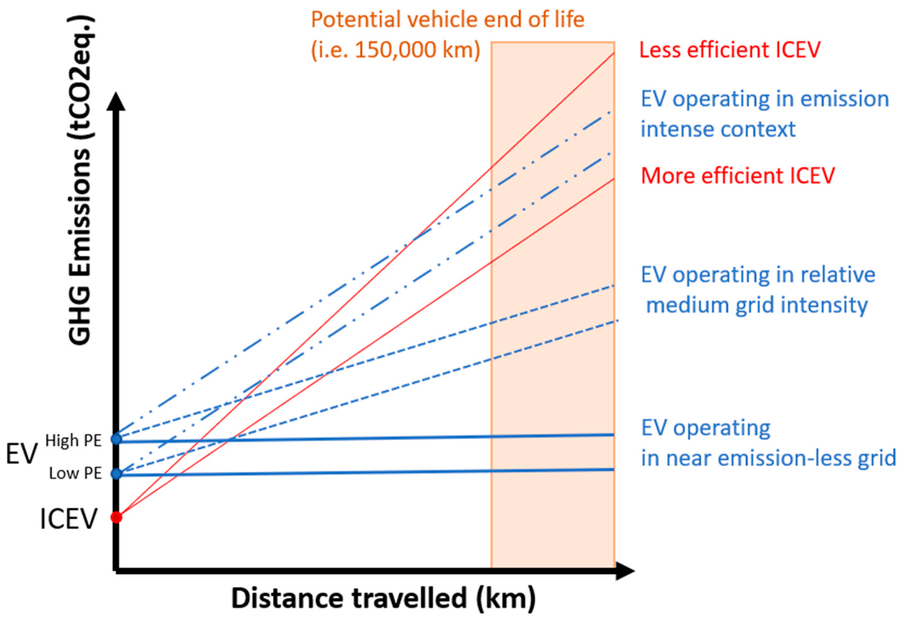
2.3.1. Distance of Intersection Point

The distance of intersection point (DIP) represents the number of kilometres at which an EV and an ICEV would have the same life cycle emissions (illustrated in Figure 1). The DIP follows a methodology used in previous studies [36,38,39]. The two main factors affecting the DIP are the production emissions (which tend to be higher for EVs) and the use-phase emissions (which tend to be higher for ICEVs). The DIP can vary from vehicle to vehicle depending on the emissions from the electricity grid, the fuel/battery efficiency, the production emissions of the vehicle in question and the drive cycle. For the purpose of this general comparison, data on efficiency and production emissions are taken from [39].

In short, the DIP (measured in 1000s km) can be used to show how quickly an EV can provide carbon mitigation as compared to an ICEV, and is calculated using the following equation:

$$\mathrm{DIP}=\frac{\mathrm{PEev} - \mathrm{PEic}}{\left(\left(\mathrm{WTWic} + \mathrm{Mic}\right)-\left(\mathrm{WTWev} + \mathrm{Mev}\right)\right)}$$

(3)

where PE represents the production emissions, WTW represents the well-to-wheel emissions and the M the maintenance emissions of an EV and an ICEV respectively, all measured in tCO₂eq. The WTW emissions of an EV are calculated by multiplying the emissions factor of the grid with the assumed efficiency of the vehicle. This DIP calculation assumes a constant grid emissions intensity. This limitation is relaxed later in the paper as described in the next section.

2.3.2. Emissions Disparity

The emissions disparity (ED) follows a similar logic to the DIP, except instead of calculating the distance at which emissions for an EV and ICEV are equal, it measures the difference in emissions (tCO₂eq) after a certain distance driven. In this case, it looks at the disparity at the end of the vehicles’ assumed lifetime (measured in km), following the methodology developed by Dillman et al. [39]. It is calculated using this equation:

$$\mathrm{ED}=\left(\mathrm{PEic} +\left(\mathrm{WTWic}+\mathrm{Mic}\right)\times \mathrm{LT}+\mathrm{EOLic}\right)-\left(\mathrm{PEev}+\left(\mathrm{WTWev}+\mathrm{Mev}\right)\times \mathrm{LT}+\mathrm{EOLev}\right)$$

(4)

The inputs are similar to the above formula, with the addition of LT for lifetime and EOL for the end-of-life emissions (tCO₂eq) associated with the disposal and recycling processes of the different vehicle types. A positive ED means that an EV has lower emissions than an ICEV.

A modified version of the ED which considers the vehicle fleets of the three countries is calculated as well. In this weighted ED, the final number is adjusted for the share of diesel and petrol vehicles in the fleet.

2.4. Temporal Dynamics

2.4.1. Decarbonising Electricity Grids

Both national and regional governments have committed to reducing emissions from electricity production. Sixteen U.S. states and Washington D.C. have set targets for 100% clean or renewable energy [62]. These targets vary from 2030 in Rhode Island to 2070 in Arizona.

At the national level, Canada’s climate plan, published in 2020, requires 90% of electricity to come from non-emitting sources by 2030, up from 80% today [63]. In the United States, the federal government has proven to be more ambitious than most states, with a commitment to electricity that is 100% free of carbon pollution by 2035 [64]. However, according to the Energy Information Administration’s Annual Energy Outlook the USA will only have reached 44% renewable energy by 2050 with its current policies [65].

Meanwhile, according to a report by its Centro Nacional de Control de Energía, Mexico has committed to increasing its share of renewable electricity from 25% in 2019 to 40% by 2032 [54]. This is a modification of the original target, which the Mexican government admitted would not be attained.

The variability of these commitments makes it difficult to draw direct comparisons between nations and regions at a certain time in the future. Consequently, this study instead compares the EPIs between nations in 2019 and the date of their commitment (2032 for Mexico, 2030 for Canada, and 2035 for the USA). However, for Mexico and the United States, projections of electricity production (which are not necessarily in line with targets) are be used to visualise the change in EV WTW emissions over the coming decades. These projections are from the Energy Information Administration [65] for the USA and the Energy Secretariat’s Development Programme [66] for Mexico.

2.4.2. Increasing Fuel Efficiency

According to a review of global studies undertaken by the International Energy Agency, global WTW emissions (gCO₂eq/km) from petrol vehicles are expected to decrease by 32% and those from diesel vehicles to decrease by 25% between 2019 and 2030 [67]. This refers to the fuel efficiency of vehicles sold in the respective years, and therefore only impacts new vehicles.

2.4.3. Battery Production and Technology

Historically, the literature on emissions from battery production has examined only small-scale production, ignoring developments in production technology [68]. In reality, the average battery production factory has grown from a yearly capacity of 0.5 GWh of batteries in 2015 to 7.3 GWh in 2020, and this is projected to grow to 18.9 GWh by 2029 [69]. Continued upscaling could lead to a 45–55% reduction in battery production emissions, with a significant impact on EV lifecycle emissions [68]. Consequently, Section 3.3 shows variations in the DIP of EVs and ICEVs, taking into account projected changes in fuel efficiency and battery production.

Additionally, approximately half of the emissions from battery production are based on the electricity mix used during the production process [70]. Therefore, as electricity grids become less carbon intensive, battery production is expected to become less carbon intensive as a result, with similar effects seen for traditional ICEV manufacturing in terms of electricity use in production.

There are other developments in production, technology, efficiency, and recycling that could affect the emissions from batteries. However, these are harder to project into the future, and are not analysed here. Further information on these sectors can be found in Section 4.5.

3. Results

This study shows that in nations and regions with lower EFs the carbon mitigation potential of EVs is accordingly higher. At the national level, Canada is the best performer, with Mexico and the USA having comparable results. At the state/province level, Québec is by far the best performer due to its largely hydropower electricity generation, followed by South Dakota, Vermont, and Washington. Alaska and Iowa were the worst performers; in these states, DIPs for diesel and petrol ICEVs did not exist due to high grid carbon intensities. A Monte Carlo simulation was performed as a sensitivity analysis, and can be found in Appendix C. The Monte Carlo simulation showed a 90% certainty of an EV leading to emissions reduction over a diesel or petrol vehicle below an electricity emission factor of ~450 and ~700, for diesel and petrol respectively.

This chapter first examines the national results before examining the state and provincial results in detail, followed by a review of the changes caused by decarbonising electricity grids and improved fuel and battery technology.

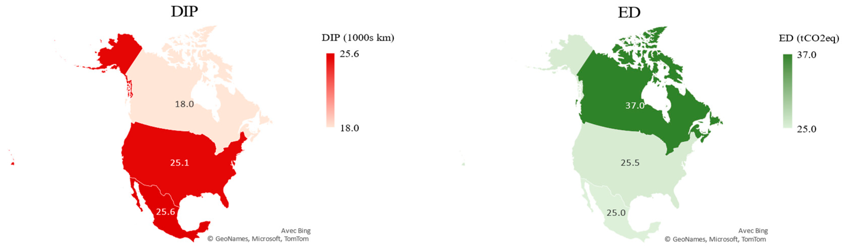
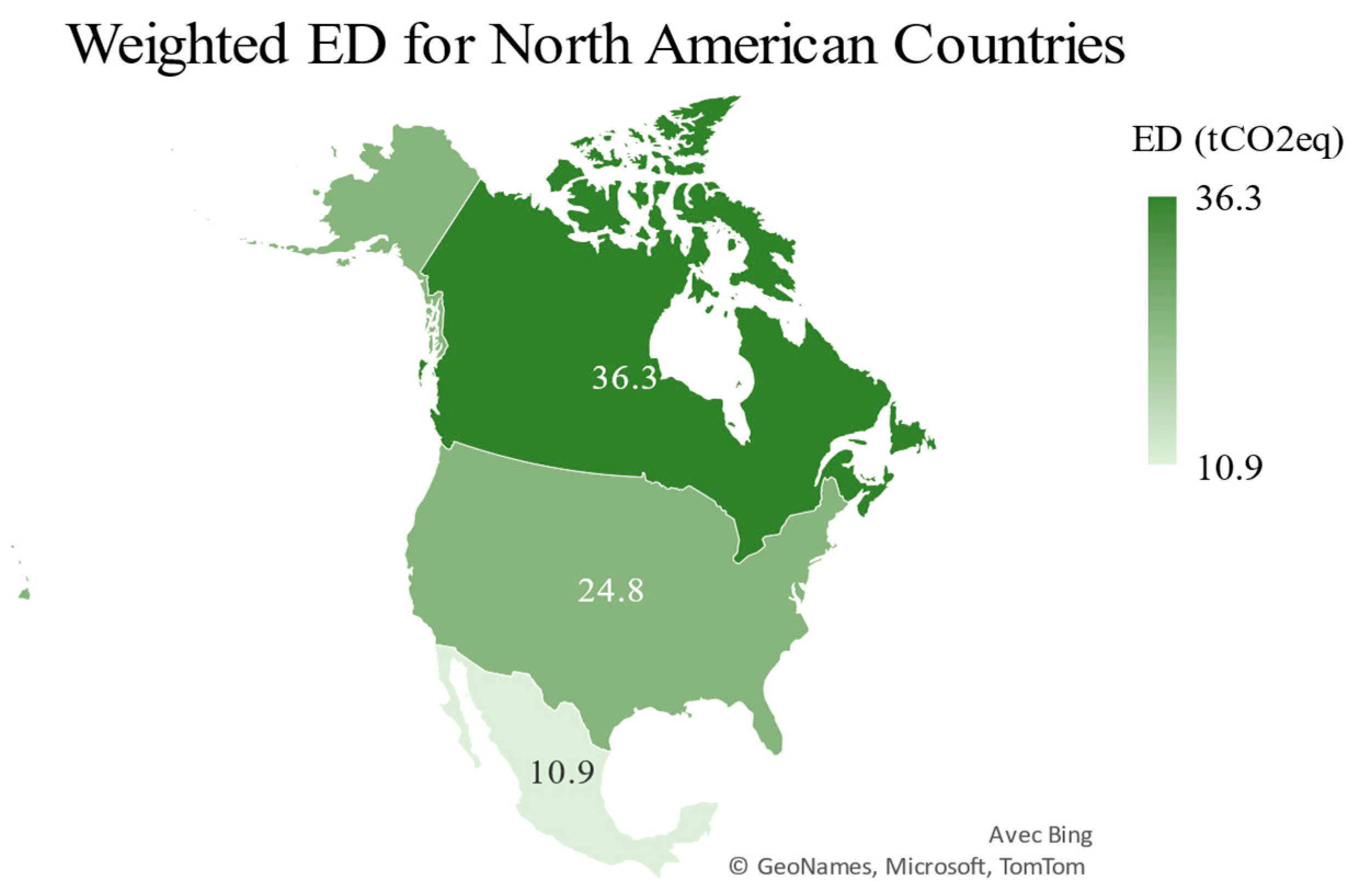
3.1. National Results

Canada’s electricity grid was estimated to have an EF of 103 gCO₂eq/kWh, while the USA and Mexico electricity grids EFs were estimated to be 476 and 494 gCO₂eq/kWh, respectively. This translates to better environmental performance for EVs in Canada than in the USA and Mexico, as can be seen in Figure 2.

Furthermore, the DIP in Canada was estimated to be 18,034 km for a petrol vehicle and 34,281 km for a diesel vehicle, while the DIP for petrol vehicles in the USA and Mexico was 25,777 km and 25,558 km, respectively. The difference was even more marked for diesel vehicles, which had a DIP of 62,827 km in the USA and 65,547 km in Mexico. This means that an owner of an EV in one of these two countries would have to drive almost double the distance of a Canadian EV owner to reach the environmental breakeven point with a diesel vehicle.

All three countries have positive EDs for both petrol and diesel vehicles, meaning that over their lifetime EVs have lower emissions than ICEVs. However, there is significant variation. In Mexico and the USA, a diesel ICEV emits 8 tCO₂eq more than an EV, while in Canada this reaches 20 tCO₂eq. For petrol ICEVs, Mexico and the USA have EDs of 25 and 26 tCO₂eq, respectively, compared to 37 tCO₂eq in Canada. This means that the mitigation potential of EVs in Mexico, where 81% of the vehicle fleet uses diesel, could be far lower [71]. To illustrate this, Figure 3 shows a map with the average of the petrol and diesel EDs weighted according to the share of vehicles in each country that use that fuel. In this weighted scenario, it becomes apparent that switching to EVs may have less of an impact on GHG emissions in Mexico than in the USA and Canada at the current electricity EF.

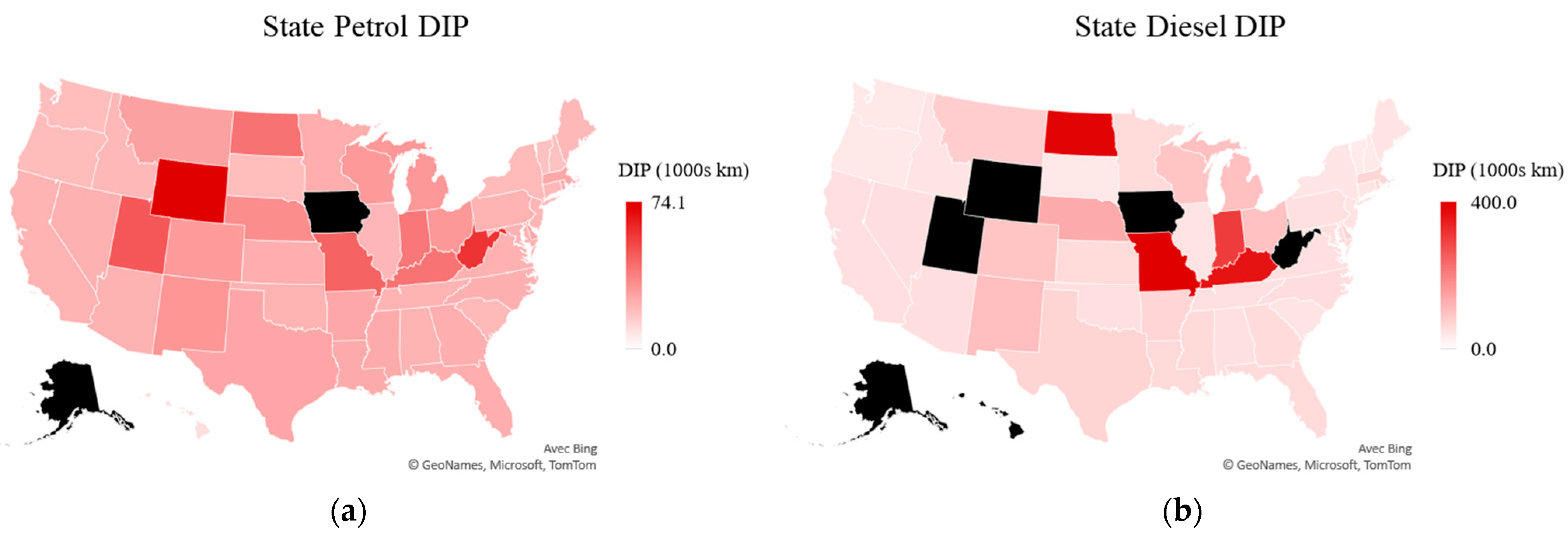
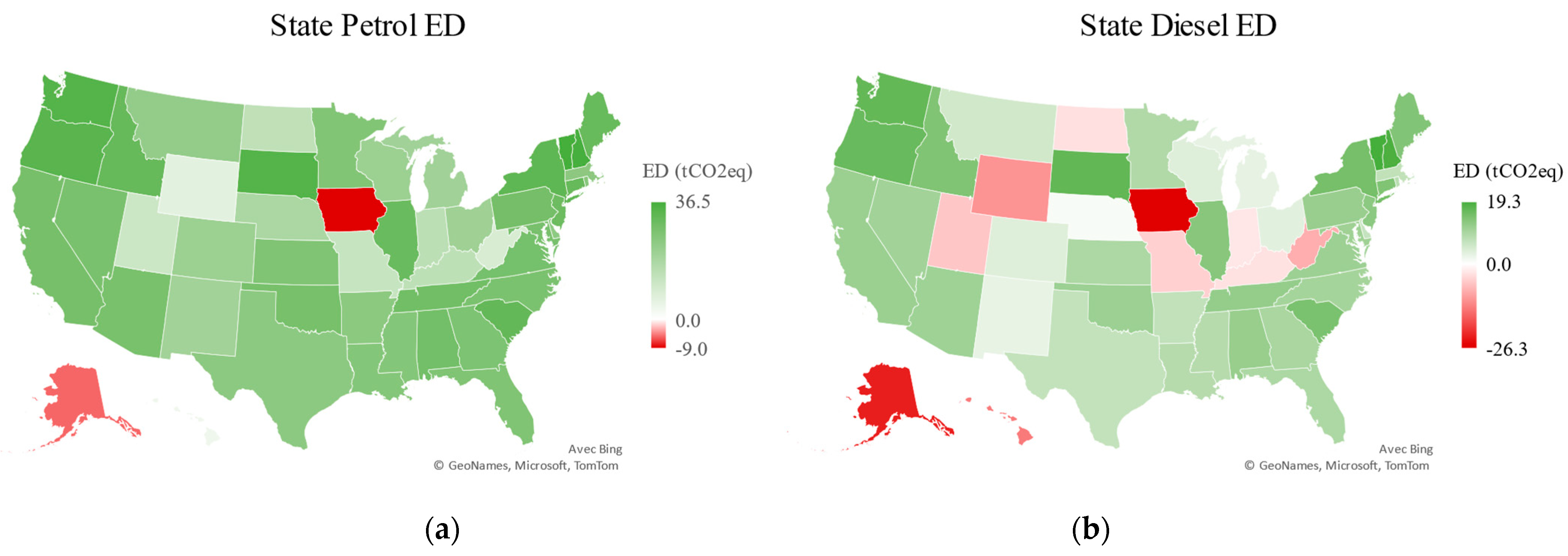
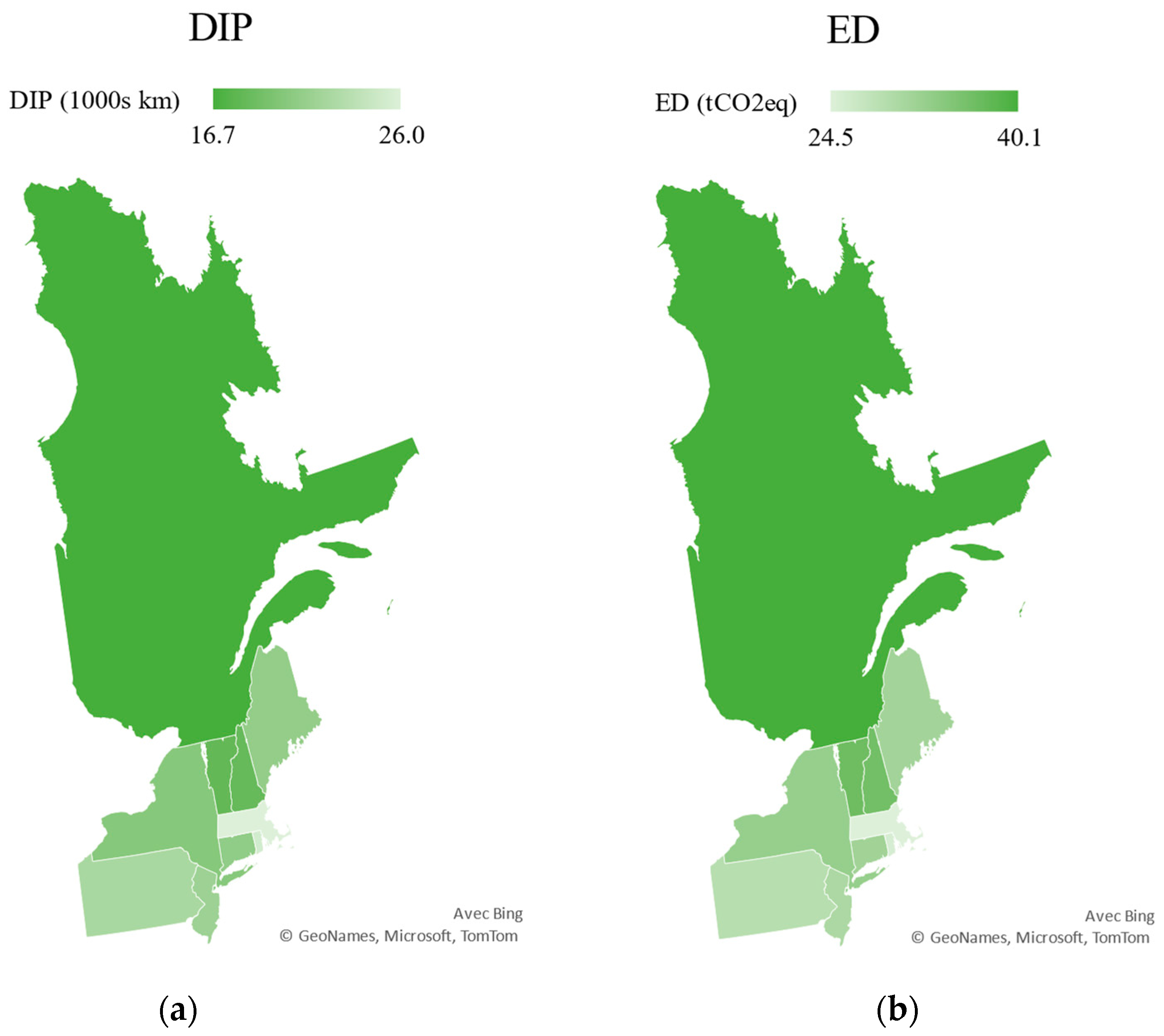
3.2. Regional Results

This section first describes results for U.S. states, then includes Québec. As shown in Figure 4, in general, the DIP for petrol was significantly lower than for diesel. In fact, of all the states that had a DIP, the highest for petrol was Hawaii, where an EV needs to drive 100,000 km before intersecting with a petrol vehicle. For diesel, this number soars to 1,400,000 km in Missouri, far beyond the lifetime of a vehicle. Alaska and Iowa never reach the break-even point for petrol vehicles, whereas for diesel vehicles this list includes Hawaii, Utah, West Virginia, and Wyoming.

At the other end of the spectrum, the best-performing states are New Hampshire, Oregon, South Dakota, Vermont, and Washington State, where fewer than 40,000 km and 20,000 km need to be driven to break even with a diesel and petrol vehicle, respectively.

Concerning ED, Figure 5 shows that over an assumed lifetime of 184,000 km [29] only Alaska and Iowa have a negative ED, although Hawaii is almost neutral. As for diesel, nine states have a negative ED. Meanwhile, in Vermont, EVs have an emissions disparity of 19.3 tCO₂eq over their lifetime when compared to a diesel vehicle and 36.5 tCO₂eq when compared to a petrol vehicle.

Considering the low emissions factor of electricity in Québec, this province outperforms every single U.S. state. As seen in Figure 6, Québec sees greater mitigation potential than even Vermont and New Hampshire. Figure 6 shows the results for a petrol vehicle, and the same is true of a diesel vehicle.

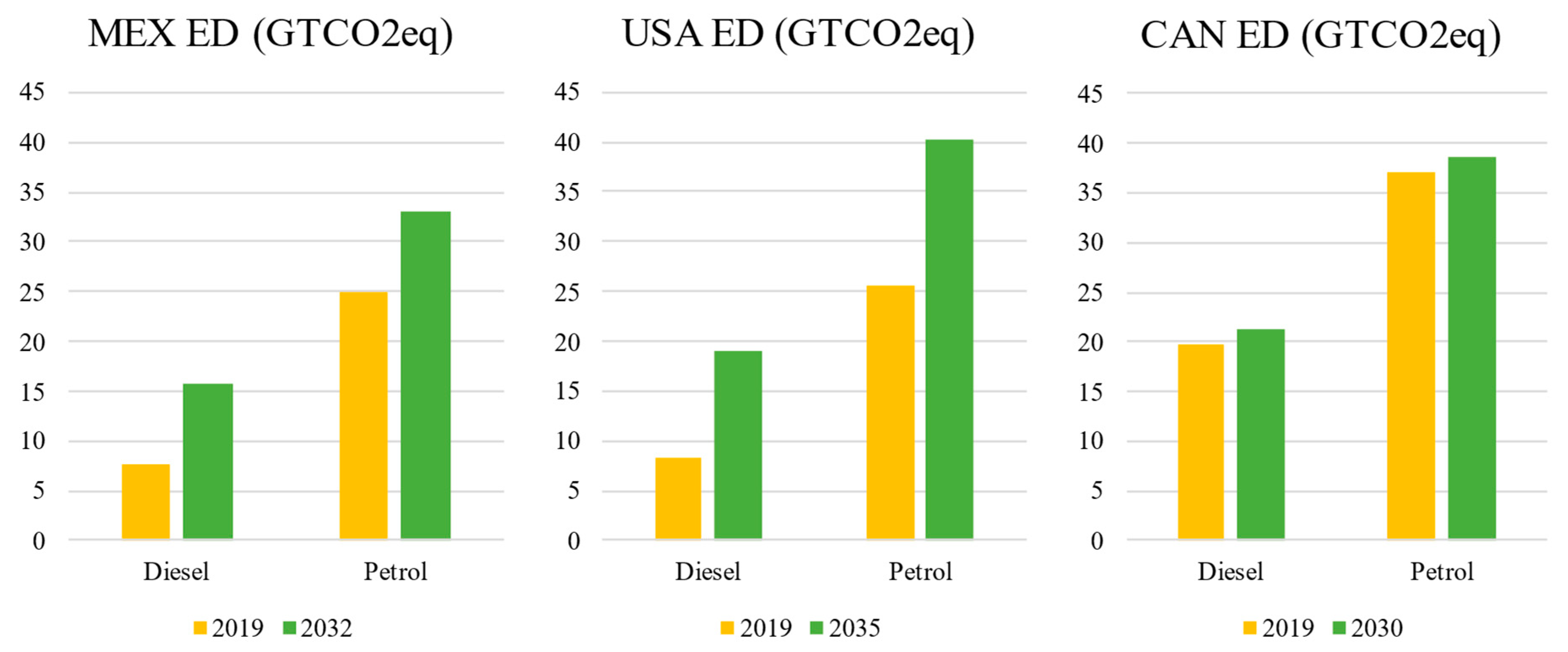
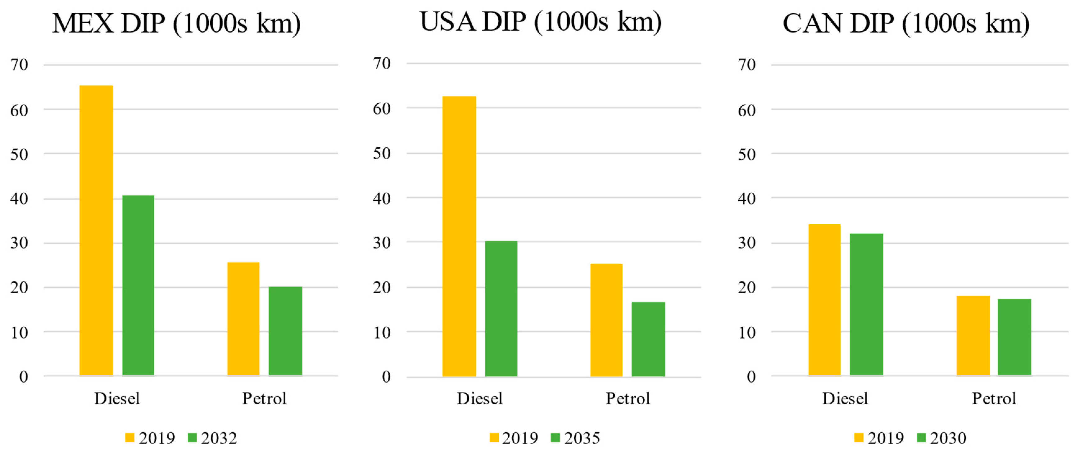
3.3. Shifting Temporal Dynamics

3.3.1. Decarbonising Grids

The three nations have each set different targets for decarbonising their electrical grids. Mexico has pledged an increase of renewable electricity from 25% in 2019 to 40% by 2032. Assuming no emissions from renewable electricity and that the remaining electricity remains equally distributed among other sources, Mexico’s EF would drop from 494 to 233 gCO₂eq/kWh, in turn leading to improved environmental performance, as illustrated in Figure 7 and Figure 8.

The largest difference is the 104% increase in the ED of diesel vehicles, while the petrol ED increases by 32%. As for the DIPs, there is a 38% decrease in the required km to outperform a diesel vehicle and a 22% decrease for a petrol vehicle.

Canada’s decarbonisation commitments would cause the EF to halve from 103 to 51.5 gCO₂eq/kWh. Unsurprisingly, this leads to increased mitigation potential for EVs in Canada.

As illustrated in Figure 7 and Figure 8, the ED in Canada increases by 4% against a petrol vehicle and 8% against a diesel vehicle, meaning that at the end of the vehicle’s lifetime, an EV would have saved an additional 4–8% of GHG emissions compared to an equivalent ICEV. Meanwhile, the DIP shows similar trends, with a 6% and 4% decrease for diesel and petrol vehicles, respectively.

Meanwhile, if the USA’s goal of using 100% NEES by 2035 is achieved, it would lead to an EF of 0 gCO₂/kWh. This is a lofty commitment, and if attained would have significant impacts on the environmental performance of EVs in the USA.

As can be seen in Figure 7 and Figure 8, by 2035 the diesel ED nearly triples, with an increase of 177%, while the petrol ED increases by 57%. The DIP accordingly decreases by 52% and 33% for diesel and petrol, respectively.

The above results are based on pledges made by the different governments. However, reality may not follow these pledges, and while Canada is on track for its target, projections for the American and Mexican grids show a significant difference from their respective pledges. These are shown separately below due to the differences in their time scales. For example, while the USA has pledged to have 100% carbon-free electricity by 2035, according to projections in the annual energy outlook this figure will only be 51% [65]. This would lead to a decrease in WTW emissions from over 140 gCO₂eq/km in 2010 to under 40 gCO₂eq/km in 2050, with a significant drop between 2010 and 2025, and a slower reduction in WTW emissions from 2025.

Meanwhile, in Mexico, the reduction is slightly slower. Following projections from Mexico’s Energy Secretariat [66], WTW emissions should decrease from 82.5 gCO₂eq/km in 2020 to 54.3 gCO₂eq/km in 2036. This is a smaller decrease than in the USA, where WTW emissions fall from 79.5 gCO₂eq/km in 2020 to 43.4 gCO₂eq/km in 2035. However, unlike the USA, the Mexican projections do not appear to level off. If projected trends were to continue, the WTW emissions would reach between 24.6 and 30.1 gCO₂eq/km in 2050, compared to 38.7 gCO₂eq/km in the USA.

3.3.2. Fuel Efficiency and Battery Production

This subsection looks at three scenarios: a low-emissions fuel scenario, a low-emissions battery production scenario, and a scenario with both factors. In the low-emissions fuel scenario, diesel emissions drop from 154.3 to 115.7 gCO₂eq/km and petrol emissions fall from 237.1 to 161.2 gCO₂eq/km. In the second scenario, emissions from EV production decrease from 10.2 to 8.1 tCO₂eq.

If the IEA’s estimates for the decrease in emissions from petrol and diesel are accurate, then the mitigation potential of EVs will decrease. Colorado, Delaware, Michigan, Montana, Nebraska, New Mexico, Ohio, Texas, and Wisconsin would subsequently all gain negative EDs for diesel vehicles, while Hawaii, Utah, Missouri, West Virginia, and Wyoming would all gain negative EDs for petrol vehicles.

In this low-emissions fuel scenario, the DIPs of EVs and ICEVs increase significantly. As can be seen in Figure 9a, eleven states will never intersect, and five additional states will require more than 400,000 km to be driven for equivalent emissions.

Our second scenario sees upscaling of battery production and greener electricity leading to a 25% reduction in production phase emissions. In this scenario, shown in Figure 9b, EDs increase across the board, and the state of Indiana passes from a negative to a positive diesel ED.

In this scenario, there is a significant decrease in DIPs. For petrol vehicles, while there is still no intersection for Alaska and Iowa, for all other states the DIP drops to less than a third of the value of the standard scenario. For example, in Hawaii, an EV owner would only need to drive 32,000 km instead of 100,000, and in Québec it drops from 17,000 km to 5000.

The final scenario assumes both increased fuel efficiency and reduced EV production emissions, leading to mixed results. For example, in Québec the DIP decreases, which indicates improved environmental performance; however, the ED decreases, meaning that at the end of the vehicle’s life it has had less of an impact. In fact, the diesel ED decreases by 4.4 GtCO₂eq and the petrol ED decreases by 11.3 in every state in this scenario. The DIP is more variable; for example, in the state of Colorado the DIP with a diesel vehicle increases by 68,000 km, while the DIP with a petrol vehicle decreases by 8000 km. On average, environmental performance does increase in this scenario; however, there is a large disparity between the states.

Lastly, it is important to stress that in all three scenarios the overall emissions decrease, which is positive; it is only the comparative performance of the vehicles that is better or worse.

4. Discussion

This study set out to compare the lifecycle emissions of electric vehicles and internal combustion engine vehicles in North America and to analyse how these are affected by the temporal dynamics. This was achieved by calculating the EFs of the electricity grids for Canada, Mexico, and the USA, as well as the 50 U.S. states, Washington D.C., and Québec. This EF was then used to calculate the DIP and ED. Different scenarios were then studied according to projected variations in vehicle production and well-to-wheel emissions.

4.1. Grid Carbon Intensity and Life Cycle Emissions

The first research question asked how the GHG intensities of the electric grids across North America affect the life cycle emissions, DIPs, and EDs of EVs in comparison to ICEVs. As an overall answer, according to our analysis all three countries would benefit from electrification of their vehicle fleets.

The results shown in Section 3.1 and Section 3.2, however, show that higher carbon intensity of the electrical grid significantly impacts the lifecycle emissions of EVs. This matches results from several previous studies [38,39,41], all of which found GHG emissions from EVs to be lower in areas with strong renewable energy infrastructure. In states, such as Alaska and Iowa, which have significantly carbon intensive grids, EVs were estimated to have higher emissions than ICEVs.

Canada, in particular, would see a substantial reduction in emissions following EV adoption. While Mexico and the USA have similar EFs, when looking at their vehicle fleets in further detail the potential benefits are different. In the USA, only 1.5% of light duty vehicles sold in 2014 used diesel; meanwhile, in Mexico diesel vehicles account for over 80% of the passenger vehicle fleet [71,72]. Considering that the emissions disparity of an EV at the end of its lifetime is much higher compared to petrol vehicles than to diesel vehicles, a switch to EVs would have a much larger impact in the petrol-heavy United States than in diesel-dominated Mexico.

The regional results show that although EV penetration leads to overall reductions, it leads to increased emissions in certain areas. However, while the results at the state level found at least two states where EVs would cause more GHGs than a petrol ICEVs, Woody et al. [41] found that the same was true in only 1–2% of counties. This shows how localised mitigation results can be within the interconnected continental grid. The regional results show that strong renewable regional infrastructure can lead to excellent environmental performance from EVs, as is the case in Québec, which has over 99% clean electricity. This significant regional disparity is to be expected in large federated countries such as Canada, Mexico, and the United States.

4.2. Temporal Dynamics

The second research question asked how grid decarbonisation, fuel efficiency improvements, and less GHG-intensive production affects the metrics described above. In all of the studied aspects, the temporal dynamics led to reduced emissions. While all three countries have set targets to reduce emissions from electricity, the U.S. commitment to 100% emissions-free electricity by 2035 would lead to the greatest reduction in emissions; if achieved, it will more than double the current emissions savings from EV use. This clearly highlights how reducing the emission intensity of electricity production must go hand in hand with the electrification of transport in order to increase emission reduction potential. This is especially important in regions with extremely high transport emissions per capita [3].

Meanwhile, fuel efficiency and improved battery production lead to reduced emissions. This can have mixed impacts on the relative environmental performance of EVs. For example, in Colorado these reductions lead to an increase in the DIP of a diesel vehicle and a decrease in the DIP of a petrol vehicle. This depends on the carbon intensity of the grid, which emphasises even further the importance of reducing emissions from electricity production.

However, when considering the above temporal dynamics, it is important to realise the context of these reductions in emissions. The improved efficiency and battery production only apply to new vehicles, and as such will take a long time to manifest across an aging vehicle fleet [73]. It is important in this case that new EVs replace older inefficient ICEVs and that incentives be in place to encourage this. Meanwhile, grid decarbonisation applies directly to any EVs currently on the road. This indicates a clear priority for policy makers who want to rapidly reduce emissions. It is worth remembering that even the most fuel efficient ICEV, and even an EV produced and operating in a 100% clean grid, will have more emissions than no vehicle at all.

Furthermore, if population growth continues and vehicle ownership rates stay the same, the number of EVs required will increase dramatically, and electricity production would need to increase accordingly. Canada’s climate plan estimates that the country may need to triple its non-emitting power generation by 2050 in order to keep up with electrification [63].

The amount of energy and resources required to produce the infrastructure for this huge electricity generation could have serious impacts on the planet’s ecosystems. This needs to be taken into account when planning future transport policies. In fact, it is estimated that if all the vehicles in the world were to become electric, electricity generation would need to increase by 18%, and this figure increases to 29% in the USA [74]. In Iceland, Dillman et al. [75] estimated that deep transport sector decarbonization is only possible if an important component of the development in the sector includes a reduction in the size of the vehicle fleet. According to them, EV penetration alone is not sufficient even in the case of Iceland, where electricity is fully renewables-based. Moreover, these results do not account for the upgrades in transport and electricity generation infrastructure and grid capacity that would be required.

4.3. Limitations and Future Research

The first and arguably most important limitation of this study is a lack of accurate information on electricity trading across state and national borders. Using the example of California, which is the largest importer of electricity in the USA [76], this study assumed that its electricity came equally from all across the USA. However, in reality California is more likely to import electricity from nearby states. However, as data were not available on specific interstate trade this assumption could not be confirmed. The same is likely true for other states, and to a lesser extent the national grids; for instance, whether electricity was imported from Québec or Ontario would change the final EF. Further, while in this study we benchmarked our analysis to the decarbonization plans of each country, plans and reality have been shown to often not coincide. While the scope of our work incorporated stated plans and projections based on the current status, future studies could consider various scenarios which stray from the stated goals to reflect various pathways.

The second primary limitation is that we used an average vehicle, drive cycle, and charge cycle. There is likely to be huge variation according to vehicle weight, production emissions (based on location, parts used, recycle rates, etc.), changing vehicle fleets, marginal vs. average emissions factors, and more. If marginal emission factors are taken into account, the actual environmental benefit could be as much as 20% lower than anticipated, although charging plans can easily be developed to reduce marginal emissions from EV charging [77,78]. In order to account for this we used the average emission factors, and provide a sensitivity analysis to consider the potential movement in either direction. Further study on the influence of charging behaviour on final emissions is needed. Furthermore, the behavioural aspects of EVs within the context of their operation are critical to their environmental performance. While [41] found that vehicle class did not affect proportionate emissions, it does affect overall emissions, and as such future research could investigate vehicle fleet composition and total mitigation potential. Energy management within the vehicles themselves under various driving conditions can be further optimized for increased efficiency as well, and would further increase the mitigation potential of EVs [79,80].

When considering ICEVs, while supply chains, technology, efficiency, and recycling improvements were taken into account, we did not consider the spatial variation of transport emissions for the various fuels or technological developments such as carbon capture and storage (CCS) in fossil fuel supply chains. For the first point, transport emissions generally comprise <1% of a fossil fuel vehicle’s life cycle emissions (where extraction, refining, and combustion often compose >99%; see, e.g., [81]. Thus, even longer supply chains are unlikely to add a significant source of emissions and are unlikely to significantly impact the results. As for the second point, crude oil extraction (where CCS occurs) generally only makes up <10% of the lifecycle emissions of a functional unit of fossil fuels. Moreover, the quality of this capture has been called into question, as this sequestration is generally for the purpose of enhanced oil recovery (EOR) and places greater focus on increased oil extraction than decreased environmental impact. Such sequestration sees permanent sequestration rates from 44–85% depending on the geological conditions [82], is a developing technology with many uncertainties, and, proportional to the size of the oil and gas industry, has not been deployed at scale [83]. Thus, these two factors are unlikely to lead to more than a 5% impact on future scenarios. Instead, we focused on efficiency and supply chain decarbonization in our future scenarios as proxies for these developments.

There are many other aspects that this study did not consider. For example, it could be beneficial to weight emissions based on when they occur, as a spike in emissions now may in fact be more harmful than a slightly higher level of emissions in the long term [84,85], and future emissions are more uncertain and may be overestimated. One example of a development leading to an overestimation of emissions from future gasoline combustion is that the fuel that ICEVs consume could change and become more ecologically friendly, particularly by using biofuels.

Vehicle component recycling, smart self-driving cars, and temperature can all impact the lifetime emissions of vehicles. Other technological advancements such as the solid-state battery [86], other potentially disruptive battery technologies under development, and automated driving were not considered due to their unpredictable nature.

Lastly, it is important to mention that this study only examined GHG emissions (measured in tCO₂eq); however, both EVs and ICEVs have other environmental and social impacts. For example, ICEVs produce pollution in the form of particulate matter, which can significantly impact ecosystem diversity [87]. Meanwhile, improper disposal of used lithium batteries from EVs can have toxic effects on human and environmental health [88]. Transport-related choices affect the wellbeing of end users, with notable health impacts due to air pollution and noise pollution [89]. Lastly, electric vehicle value chains have social ramifications that should be considered [90].

Future research could aim to understand the nature of the electricity consumed in the various states, provinces, and territories of North America. As we move towards electrification in many industries, information on the source of electricity consumed will become vital. Such research could investigate the electrification of transport from a systems perspective, accounting for increased electricity production and infrastructure requirements.

4.4. Policy Recommendations

Targets for electrification of transport and financial incentives for EV adoption have been developed across all three nations. In Canada, only two provinces (Québec and British Columbia) currently offer financial incentives for EVs. These two provinces also have by far the highest share of ZEVs in their fleet, with 8.4% in B.C. and 6.8% in Québec. Meanwhile in Ontario this figure is only 1.8%, which indicates that such financial incentives truly are effective [12].

However, this research has indicated, alongside other studies [39,41,89,91], that EVs are only able to provide limited decarbonization potential in regions with high grid carbon intensities. Consequently, it is debatable whether promoting the adoption of EVs in states with highly carbon intense grids, such as Alaska and Iowa, should be a priority.

Instead, the key priority in many places should be to invest in renewable energy infrastructure before investing in EV incentives and infrastructure. Meanwhile, countries such as the USA and Mexico, which have middling emissions factors, should boost their renewable energy while continuing to offer EV incentives through targeted policies which can prioritise the uptake of EVs in the regions where they have the greatest impact. Attention, should be paid to placing new renewable energy infrastructure in places with the most carbon-heavy grids. This can be tenuous in situations such as Mexico, where protective energy policies in the current administration have led to emissions intensity backsliding [92]. Areas with low-carbon grids, such as Canada, Québec, and Oregon, can focus more on transport policies. This transport policy could follow the three pillars of an avoid–shift–improve strategy, as suggested by the literature, with a view to full-scale electrification by 2050 [75,89].

The first pillar is to avoid all unnecessary vehicle journeys and to promote active modes of transport. These are the cleanest forms of transportation, and provide health benefits to users as well [93]. Further unnecessary journeys can be avoided through the targeted promotion of teleworking [94].

The second pillar is to promote a shift away from individual vehicles. This could be through shared mobility, which can interact with micro-mobility and public transport to create effective networks. Higher occupancy in shared mobility systems leads to more effective results [89,95]. Investment in public transit is crucial, especially rail, which continues to be the least energy-demanding mode of transportation [96].

The final pillar is to improve the environmental performance of passenger vehicles, which is where EVs finally come into play. It is almost impossible for all journeys to be avoided or undertaken by public or shared transportation methods. This is especially true in vast and sparsely-populated rural areas, which have historically had less access to the public transportation networks [97].

All three countries have introduced or are introducing legislation requiring EVs to represent a certain portion of new vehicle sales. However, these policies alone are not enough, and must be part of a coordinated policy push. In fact, Mangan et al. [98] found that the implementation of current policies would only lead to 7% of the global fleet being ZEVs.

Additionally, clear information should be in place for users to know when the best time to charge their vehicle is, both in terms of emissions and cost. This information can be highly localised, as it depends on local industry and weather patterns. Policies such as the dedicated energy label suggested by Weiss et al. [99] could help to shift people towards lighter vehicles, which have significantly lower emissions.

One innovative idea is to create a fleet of shared automated electric vehicles. This would combine all three phases by reducing individual car ownership, shifting to shared transportation, and improving environmental performance. It is estimated that such a fleet could reduce GHG emissions by 70% while creating significant cost savings [100].

Lastly, in light of the large emissions from production, policies that encourage recycling and repair of vehicles to reduce production emissions should be introduced. Right to repair laws are commonplace for consumer electronics, and these could be expanded to include vehicles.

Education is another valuable tool. Many policies have focused on educating youth about the environmental impacts of GHG emissions, which has proven effective as young people are more concerned by climate change and its potential impacts [101]. This education should be expanded to raise awareness among adults.

Beyond these direct-action policies, governments and utilities could combine to produce statistics on the emissions from electricity consumption in the states and provinces. Considering that they already produce data for state electricity production emissions, as well as total consumption and electricity imports and exports, this should not be a difficult task. Access to data is key for researchers and the public to be able to make informed and appropriate decisions.

It is important to recognize the difference in capabilities as well, however; justice aspects of transitions, such as the electrification of transport, need to be considered [102,103]. This is particularly true when comparing countries with significant differences in economic development; for instance, Mexico has populations suffering from energy and transport poverty, and significant socio-economic and justice developments would be needed before high levels of electrification across society could be expected [104].

4.5. Concluding Remarks

This study quantified the environmental performance of EVs in North America to assess their effectiveness across time and space according to various operating conditions. The work included an assessment of electrical grid GHG intensities taking into account trade in the U.S. and modelling of decarbonization pathways aligned with national policies for the three North American countries. It then assessed the distance of intersection point and emission disparity both nationally and regionally for the three countries (primarily in the US). This study found that over its lifetime an EV produces lower emissions than either a petrol or diesel ICEV in all three nations. Canada was the best performer at the national level, and Québec, where almost all electricity comes from renewable sources, saw the greatest mitigation potential. In Québec there is only 0.1 gCO₂eq released for every kWh of electricity generated, which means that over its lifetime an EV would emit 23 tons of CO₂eq less than a diesel vehicle and 40 tons less than a petrol vehicle. Both Mexico and the USA saw positive overall impacts from EVs compared to both types of fuel ICEV. At the regional level in the USA the worst performer was Iowa, where an EV would produce 9 tCO₂eq more than a petrol vehicle and 26 tCO₂eq more than a diesel vehicle. Other states with negative impacts were Alaska, Hawaii, Utah, West Virginia, and Wyoming, where EVs were never able to outperform a diesel ICEV.

This diversity in results calls for an equally diverse set of policies for tackling emissions from transport. This diverse policy framework should adapt itself to local conditions, and should follow the ASI framework suggested by the IEA, among others. This should be done within a consumer-friendly environment in which there is easy access to data and transport services such as roads and public transit, widespread education, and good options for repairing and reusing vehicles. Electric vehicles are often considered a silver bullet for reducing greenhouse gas emissions; however, the reality is that they are only one part of a substantial change required across transport and energy systems, both in North America and the rest of the world.

References

1. Steffen, W. Introducing the Anthropocene: The Human Epoch: This Article Belongs to Ambio’s 50th Anniversary Collection. Theme: Anthropocene. Ambio 2021, 50, 1784–1787. [Google Scholar] [CrossRef]
2. WMO. United in Science 2021: A Multi-Organization High-Level Compilation of the Latest Climate Science Information; World Meteorological Organization (WMO); United Nations Environment Programme; Intergovernmental Panel on Climate Change; United Nations Educational, Scientific and Cultural Organization (UNESCO); Intergovernmental Oceanographic Commission (IOC); Global Carbon Project; WMO: Geneva, Switzerland, 2021. [Google Scholar]
3. Lamb, W.F.; Wiedmann, T.; Pongratz, J.; Andrew, R.; Crippa, M.; Olivier, J.G.J.; Wiedenhofer, D.; Mattioli, G.; Al Khourdajie, A.; House, J.; et al. A Review of Trends and Drivers of Greenhouse Gas Emissions by Sector from 1990 to 2018. Environ. Res. Lett. 2021, 16, 073005. [Google Scholar] [CrossRef]
4. Ritchie, H.; Roser, M. CO2 and Greenhouse Gas Emissions. Available online: https://ourworldindata.org/co2-and-other-greenhouse-gas-emissions (accessed on 15 November 2022).
5. O’Neill, D.W.; Fanning, A.L.; Lamb, W.F.; Steinberger, J.K. A Good Life for All within Planetary Boundaries. Nat. Sustain. 2018, 1, 88–95. [Google Scholar] [CrossRef] [Green Version]
6. Wang, S.; Ge, M. Everything You Need to Know about the Fastest-Growing Source of Global Emissions: Transport; World Resources Insitute: Washington, DC, USA, 2019. [Google Scholar]
7. IEA Global Energy Review. 2021. Available online: https://www.iea.org/reports/global-energy-review-2021 (accessed on 20 February 2022).
8. Pathak, P.K.; Yadav, A.K.; Padmanaban, S.; Alvi, P.A. Design of Robust Multi-Rating Battery Charger for Charging Station of Electric Vehicles via Solar PV System. Electr. Power Components Syst. 2022, 50, 751–761. [Google Scholar] [CrossRef]
9. Pathak, P.K.; Yadav, A.K.; Padmanaban, S.; Alvi, P.A.; Kamwa, I. Fuel Cell-based Topologies and Multi-input DC–DC Power Converters for Hybrid Electric Vehicles: A Comprehensive Review. IET Gener. Transm. Distrib. 2022, 16, 2111–2139. [Google Scholar] [CrossRef]
10. ECCC. Rapport D’Inventaire National 1990–2019: Sources et Puits de Gaz à Effets de Serre Au Canada; Environnement et Changement Climatique Canada: Gatineau, QC, Canada, 2021.
11. Government of Canada. Canada’s 2021 Nationally Determined Contribution Under the Paris Agreement; Government of Canada: Ottawa, ON, Canada, 2021.
12. Jarratt, E. Zero-Emission Vehicle Market Share in Canada Rose to 3.5 per Cent in 2020. Available online: https://electricautonomy.ca/2021/04/23/canadian-ev-sales-data-2020/ (accessed on 8 March 2022).
13. TCP By the Numbers: A Look at Electric Vehicle Sales in Canada. Available online: https://www.thestar.com/business/2021/12/10/by-the-numbers-a-look-at-electric-vehicle-sales-in-canada.html (accessed on 15 November 2022).
14. MELCC. GES 1990–2019: Inventaire Québécois Des Emissions de Gaz à Effet de Serre En 2019 et Leur Evolution Depuis 1990; Ministère de l’Environnement et de la Lutte Contre le Changement Climatique: Québec City, QC, Canada, 2021. [Google Scholar]
15. EPA Inventory of U.S. Greenhouse Gas Emissions and Sinks: 1990–2019; United States Environmental Protecetion Agency: Washington, DC, USA, 2021.
16. EPA. Fast Facts on Transportation Greenhouse Gas Emissions; United States Environmental Protection Agency: Washington, DC, USA, 2021.
17. EIA State Carbon Dioxide Emissions Data-U.S. Energy Information Administration (EIA). Available online: https://www.eia.gov/environment/emissions/state/ (accessed on 22 February 2022).
18. IEA. Global EV Outlook 2021; International Energy Agency: Paris, France, 2021. [Google Scholar]
19. Paoli, L.; Gül, T. Electric Cars Fend off Supply Challenges to More than Double Global Sales. Available online: https://www.iea.org/commentaries/electric-cars-fend-off-supply-challenges-to-more-than-double-global-sales (accessed on 8 March 2022).
20. EVA EV Market Share by State–EVAdoption. Available online: https://evadoption.com/ev-market-share/ev-market-share-state/ (accessed on 8 March 2022).
21. Government of the USA. The United States’ Nationally Determined Contribution: Reducing Greenhouse Gases in the United States: A 2030 Emissions Target; Government of the United States of America: Washington, DC, USA, 2021.
22. US Senate. Summary of the Energy Security and Climate Change Investments in the Inflation Reduction Act of 2022; US Government: Washington, DC, USA, 2022.
23. INECC. Contribución Determinada a Nivel Nacional: Actualización 2020; Gobierno de México; Secretaría de Medio Ambiente y Recursos Naturales; Instituo Nacional de Ecologia y Cambio Climatico: Mexico City, Mexico, 2020. [Google Scholar]
24. SEMARNAT. Estrategia Nacional de Movilidad Eléctrica; Gobierno de México, Secretaría de Medio Ambiente y Recursos Naturales: Mexico City, Mexico, 2018. [Google Scholar]
25. Guglielmetti, F. En lista de espera: México aún tiene pendiente su Estrategia Nacional de Movilidad Eléctrica. Available online: https://portalmovilidad.com/en-lista-de-espera-mexico-aun-tiene-pendiente-su-estrategia-nacional-de-movilidad-electrica/ (accessed on 18 February 2022).
26. Flores, L. México Carece de Infraestructura Para Acelerar Producción de Vehículos Eléctricos: Clúster Automotriz de Nuevo León. Available online: https://www.eleconomista.com.mx/estados/Mexico-carece-de-infraestructura-para-acelerar-produccion-de-vehiculos-electricos-Cluster-Automotriz-de-Nuevo-Leon-20210526-0134.html (accessed on 8 March 2022).
27. Philippot, M.; Alvarez, G.; Ayerbe, E.; Van Mierlo, J.; Messagie, M. Eco-Efficiency of a Lithium-Ion Battery for Electric Vehicles: Influence of Manufacturing Country and Commodity Prices on GHG Emissions and Costs. Batteries 2019, 5, 23. [Google Scholar] [CrossRef] [Green Version]
28. Verma, S.; Dwivedi, G.; Verma, P. Life Cycle Assessment of Electric Vehicles in Comparison to Combustion Engine Vehicles: A Review. Mater. Today 2022, 49, 217–222. [Google Scholar] [CrossRef]
29. Lai, X.; Chen, Q.; Tang, X.; Zhou, Y.; Gao, F.; Guo, Y.; Bhagat, R.; Zheng, Y. Critical Review of Life Cycle Assessment of Lithium-Ion Batteries for Electric Vehicles: A Lifespan Perspective. eTransportation 2022, 12, 100169. [Google Scholar] [CrossRef]
30. Marmiroli, B.; Messagie, M.; Dotelli, G.; Van Mierlo, J. Electricity Generation in LCA of Electric Vehicles: A Review. NATO Adv. Sci. Inst. Ser. E Appl. Sci. 2018, 8, 1384. [Google Scholar] [CrossRef] [Green Version]
31. Hamwi, H.; Rushby, T.; Mahdy, M.; Bahaj, A.S. Effects of High Ambient Temperature on Electric Vehicle Efficiency and Range: Case Study of Kuwait. Energies 2022, 15, 3178. [Google Scholar] [CrossRef]
32. Sagaama, I.; Kchiche, A.; Trojet, W.; Kamoun, F. Improving The Accuracy of The Energy Consumption Model for Electric Vehicle in SUMO Considering The Ambient Temperature Effects. In Proceedings of the 2018 IFIP/IEEE International Conference on Performance Evaluation and Modeling in Wired and Wireless Networks (PEMWN), Toulouse, France, 26–28 September 2018; pp. 1–6. [Google Scholar]
33. Al-Wreikat, Y.; Serrano, C.; Sodré, J.R. Effects of Ambient Temperature and Trip Characteristics on the Energy Consumption of an Electric Vehicle. Energy 2022, 238, 122028. [Google Scholar] [CrossRef]
34. Burchart-Korol, D.; Jursova, S.; Folęga, P.; Korol, J.; Pustejovska, P.; Blaut, A. Environmental Life Cycle Assessment of Electric Vehicles in Poland and the Czech Republic. J. Clean. Prod. 2018, 202, 476–487. [Google Scholar] [CrossRef]
35. Li, Y.; Ha, N.; Li, T. Research on Carbon Emissions of Electric Vehicles throughout the Life Cycle Assessment Taking into Vehicle Weight and Grid Mix Composition. Energies 2019, 12, 3612. [Google Scholar] [CrossRef] [Green Version]
36. Kawamoto, R.; Mochizuki, H.; Moriguchi, Y.; Nakano, T.; Motohashi, M.; Sakai, Y.; Inaba, A. Estimation of CO2 Emissions of Internal Combustion Engine Vehicle and Battery Electric Vehicle Using LCA. Sustain. Sci. Pract. Policy 2019, 11, 2690. [Google Scholar] [CrossRef] [Green Version]
37. Hawkins, T.R.; Singh, B.; Majeau-Bettez, G.; Strømman, A.H. Comparative Environmental Life Cycle Assessment of Conventional and Electric Vehicles. J. Ind. Ecol. 2013, 17, 53–64. [Google Scholar] [CrossRef]
38. Ager-Wick Ellingsen, L.; Singh, B.; Hammer Strømman, A. The Size and Range Effect: Lifecycle Greenhouse Gas Emissions of Electric Vehicles. Environ. Res. Lett. 2016, 11, 054010. [Google Scholar] [CrossRef]
39. Dillman, K.J.; Árnadóttir, Á.; Heinonen, J.; Czepkiewicz, M.; Davíðsdóttir, B. Review and Meta-Analysis of EVs: Embodied Emissions and Environmental Breakeven. Sustain. Sci. Pract. Policy 2020, 12, 9390. [Google Scholar] [CrossRef]
40. Nordelöf, A.; Messagie, M.; Tillman, A.-M.; Ljunggren Söderman, M.; Van Mierlo, J. Environmental Impacts of Hybrid, Plug-in Hybrid, and Battery Electric Vehicles—What Can We Learn from Life Cycle Assessment? Int. J. Life Cycle Assess. 2014, 19, 1866–1890. [Google Scholar] [CrossRef] [Green Version]
41. Woody, M.; Vaishnav, P.; Keoleian, G.A.; De Kleine, R.; Kim, H.C.; Anderson, J.E.; Wallington, T.J. The Role of Pickup Truck Electrification in the Decarbonization of Light-Duty Vehicles. Environ. Res. Lett. 2022, 17, 034031. [Google Scholar] [CrossRef]
42. Onat, N.C.; Kucukvar, M.; Tatari, O. Conventional, Hybrid, Plug-in Hybrid or Electric Vehicles? State-Based Comparative Carbon and Energy Footprint Analysis in the United States. Appl. Energy 2015, 150, 36–49. [Google Scholar] [CrossRef]
43. Shafique, M.; Luo, X. Environmental Life Cycle Assessment of Battery Electric Vehicles from the Current and Future Energy Mix Perspective. J. Environ. Manag. 2022, 303, 114050. [Google Scholar] [CrossRef]
44. Onat, N.C.; Kucukvar, M. A Systematic Review on Sustainability Assessment of Electric Vehicles: Knowledge Gaps and Future Perspectives. Environ. Impact Assess. Rev. 2022, 97, 106867. [Google Scholar] [CrossRef]
45. CER. Canada’s Energy Future 2019; Canada Energy Regulator, Régie de l’Energie du Canada: Calgary, AB, Canada, 2019. [Google Scholar]
46. Brandão, M.; Heath, G.; Cooper, J. What Can Meta-Analyses Tell Us about the Reliability of Life Cycle Assessment for Decision Support? J. Ind. Ecol. 2012, 16, S3–S7. [Google Scholar] [CrossRef]
47. NCEI Climate at a Glance Statewide Mapping. Available online: https://www.ncei.noaa.gov/access/monitoring/climate-at-a-glance/statewide/mapping (accessed on 15 November 2022).
48. OEERE Fuel Economy in Cold Weather. Available online: https://www.fueleconomy.gov/feg/coldweather.shtml (accessed on 8 March 2022).
49. Lohse-Busch, H.; Duoba, M.; Rask, E.; Stutenberg, K.; Gowri, V.; Slezak, L.; Anderson, D. Ambient Temperature (20°F, 72°F and 95°F) Impact on Fuel and Energy Consumption for Several Conventional Vehicles, Hybrid and Plug-In Hybrid Electric Vehicles and Battery Electric Vehicle; SAE Technical Paper; SAE International: Warrendale, PA, USA, 2013. [Google Scholar]
50. Aljohani, T.; Alzahrani, G. Life Cycle Assessment to Study the Impact of the Regional Grid Mix and Temperature Differences on the GHG Emissions of Battery Electric and Conventional Vehicles. In Proceedings of the 2019 SoutheastCon, Huntsville, AL, USA, 11–14 April 2019; pp. 1–9. [Google Scholar]
51. Moro, A.; Lonza, L. Electricity Carbon Intensity in European Member States: Impacts on GHG Emissions of Electric Vehicles. Transp. Res. Part D Trans. Environ. 2018, 64, 5–14. [Google Scholar] [CrossRef]
52. CER. Canada’s Energy Future 2021; Canada Energy Regulator, Régie de l’Energie du Canada: Calgary, AB, Canada, 2021. [Google Scholar]
53. EIA Renewables Became the Second-Most Prevalent, U.S. Electricity Source in 2020. Available online: https://www.eia.gov/todayinenergy/detail.php?id=48896 (accessed on 5 April 2022).
54. CNCE Programa de Desarrollo Del Sistema Eléctrico Nacional 2020 a 2034. Available online: https://www.gob.mx/cenace/documentos/programa-de-desarrollo-del-sistema-electrico-nacional-2020-2034 (accessed on 30 March 2022).
55. Camba, R.; Lenero, P.O.; Scott, R. How Mexico Can Harness Its Superior Energy Abundance. Available online: https://www.mckinsey.com/industries/oil-and-gas/our-insights/how-mexico-can-harness-its-superior-energy-abundance (accessed on 18 April 2022).
56. Jochem, P.; Babrowski, S.; Fichtner, W. Assessing CO2 Emissions of Electric Vehicles in Germany in 2030. Transp. Res. Part A: Policy Pract. 2015, 78, 68–83. [Google Scholar]
57. EIA Electric Power Monthly-U.S. Energy Information Administration (EIA). Available online: https://www.eia.gov/electricity/monthly/ (accessed on 27 May 2022).
58. INDE ¿Cómo Surgió La Interconexión Eléctrica Entre Guatemala y México?–INDE. Available online: http://www.inde.gob.gt/blogs/como-surgio-la-interconexion-electrica-entre-guatemala-y-mexico/ (accessed on 2 March 2022).
59. NREL. Belize Energy Snapshot; National Renewable Energy Laboratory-United States Department of Energy: Golden, CO, USA, 2020.
60. SEMARNAT. Aviso Factor de Emision Del Sistema Electrico Nacional 2020; Gobierno de México; Secretaria de Medio Ambiente y Recursos Naturales: Mexico City, Mexico, 2021. [Google Scholar]
61. EIA State Electricity Profiles-2020. Available online: https://www.eia.gov/electricity/state/ (accessed on 23 February 2022).
62. Fields, S. 100 Percent Renewable Energy Targets by State. Available online: https://news.energysage.com/states-with-100-renewable-targets/ (accessed on 3 March 2022).
63. Government of Canada. A Healthy Environment and a Healthy Economy; Government of Canada: Ottawa, ON, Canada, 2020.
64. White House FACT SHEET: President Biden Sets 2030 Greenhouse Gas Pollution Reduction Target Aimed at Creating Good-Paying Union Jobs and Securing U.S. Leadership on Clean Energy Technologies. Available online: https://www.whitehouse.gov/briefing-room/statements-releases/2021/04/22/fact-sheet-president-biden-sets-2030-greenhouse-gas-pollution-reduction-target-aimed-at-creating-good-paying-union-jobs-and-securing-u-s-leadership-on-clean-energy-technologies/ (accessed on 3 March 2022).
65. EIA Annual Energy Outlook 2022-U.S. Energy Information Administration (EIA). Available online: https://www.eia.gov/outlooks/aeo/ (accessed on 12 April 2022).
66. SENER. Programa Para El Desarrollo Del Sistema Eléctrico Nacional; Secretaría de Energía, Gobierno de México: Mexico City, Mexico, 2022. [Google Scholar]
67. IEA. Global Fuel Economy Initiative 2021; International Energy Agency: Paris, France, 2021. [Google Scholar]
68. Chordia, M.; Nordelöf, A.; Ellingsen, L.A.-W. Environmental Life Cycle Implications of Upscaling Lithium-Ion Battery Production. Int. J. Life Cycle Assess. 2021, 26, 2024–2039. [Google Scholar] [CrossRef]
69. BMI We Are over Elon Musk’s 100 Gigafactory Target for Sustainable Energy: Do We Need a Terafactory? Available online: https://www.benchmarkminerals.com/membership/we-are-over-elon-musks-100-gigafactory-target-for-sustainable-energy-do-we-need-a-terafactory/ (accessed on 2 March 2022).
70. ICCT Effects of Battery Manufacturing on Electric Vehicle Life-Cycle Greenhouse Gas Emissions. Available online: https://theicct.org/publication/effects-of-battery-manufacturing-on-electric-vehicle-life-cycle-greenhouse-gas-emissions/ (accessed on 8 March 2022).
71. Statista Passenger Vehicle Fleet in Mexico by Fuel Type. Available online: https://www.statista.com/statistics/825156/passenger-vehicle-fleet-size-units-mexico-fuel/ (accessed on 17 March 2022).
72. Chambers, M.; Schmitt, R. Fact Sheet: Diesel-Powered Passenger Cars and Light Trucks; U.S. Department of Transportation, Bureau of Transportation Statistics: Washington, DC, USA, 2015.
73. Ferris, R. Cars on American Roads Keep Getting Older. Available online: https://www.cnbc.com/2021/09/28/cars-on-american-roads-keep-getting-older.html (accessed on 22 March 2022).
74. Andrews, R. How Much More Electricity Do We Need to Go to 100% Electric Vehicles? Available online: http://euanmearns.com/how-much-more-electricity-do-we-need-to-go-to-100-electric-vehicles/ (accessed on 6 April 2022).
75. Dillman, K.; Czepkiewicz, M.; Heinonen, J.; Fazeli, R.; Árnadóttir, Á.; Davíðsdóttir, B.; Shafiei, E. Decarbonization Scenarios for Reykjavik’s Passenger Transport: The Combined Effects of Behavioural Changes and Technological Developments. Sustain. Cities Soc. 2021, 65, 102614. [Google Scholar] [CrossRef]
76. EIA California Imports the Most Electricity from Other States; Pennsylvania Exports the Most. Available online: https://www.eia.gov/todayinenergy/detail.php?id=38912 (accessed on 6 April 2022).
77. Thind, M.P.S.; Wilson, E.J.; Azevedo, I.L.; Marshall, J.D. Marginal Emissions Factors for Electricity Generation in the Midcontinent ISO. Environ. Sci. Technol. 2017, 51, 14445–14452. [Google Scholar] [CrossRef]
78. Tu, R.; Gai, Y.J.; Farooq, B.; Posen, D.; Hatzopoulou, M. Electric Vehicle Charging Optimization to Minimize Marginal Greenhouse Gas Emissions from Power Generation. Appl. Energy 2020, 277, 115517. [Google Scholar] [CrossRef]
79. Xu, X.; Zhao, J.; Zhao, J.; Shi, K.; Dong, P.; Wang, S.; Liu, Y.; Guo, W.; Liu, X. Comparative Study on Fuel Saving Potential of Series-Parallel Hybrid Transmission and Series Hybrid Transmission. Energy Convers. Manag. 2022, 252, 114970. [Google Scholar] [CrossRef]
80. Dong, P.; Zhao, J.; Liu, X.; Wu, J.; Xu, X.; Liu, Y.; Wang, S.; Guo, W. Practical Application of Energy Management Strategy for Hybrid Electric Vehicles Based on Intelligent and Connected Technologies: Development Stages, Challenges, and Future Trends. Renew. Sustain. Energy Rev. 2022, 170, 112947. [Google Scholar] [CrossRef]
81. Morales, M.; Gonzalez-García, S.; Aroca, G.; Moreira, M.T. Life Cycle Assessment of Gasoline Production and Use in Chile. Sci. Total Environ. 2015, 505, 833–843. [Google Scholar] [CrossRef] [PubMed]
82. Olea, R.A. CO2 Retention Values in Enhanced Oil Recovery. J. Pet. Sci. Eng. 2015, 129, 23–28. [Google Scholar] [CrossRef]
83. Zapantis, A.; Al Amer, N.; Havercroft, I.; Ivory-Moore, R.; Steyn, M.; Yang, X.; Gebremedhin, R.; Zahra, M.A.; Pinto, E.; Rassool, D.; et al. Global Status of CCS 2022; Global CCS Institute: Melbourne, Australia, 2022. [Google Scholar]
84. Säynäjoki, A.; Heinonen, J.; Junnila, S. A Scenario Analysis of the Life Cycle Greenhouse Gas Emissions of a New Residential Area. Environ. Res. Lett. 2012, 7, 034037. [Google Scholar] [CrossRef]
85. Kendall, A.; Price, L. Incorporating Time-Corrected Life Cycle Greenhouse Gas Emissions in Vehicle Regulations. Environ. Sci. Technol. 2012, 46, 2557–2563. [Google Scholar] [CrossRef]
86. Braga, M.H.; Grundish, N.S.; Murchison, A.J.; Goodenough, J.B. Alternative Strategy for a Safe Rechargeable Battery. Energy Environ. Sci. 2017, 10, 331–336. [Google Scholar] [CrossRef]
87. EPA Health and Environmental Effects of Particulate Matter (PM). Available online: https://www.epa.gov/pm-pollution/health-and-environmental-effects-particulate-matter-pm (accessed on 9 January 2022).
88. Kang, D.H.P.; Chen, M.; Ogunseitan, O.A. Potential Environmental and Human Health Impacts of Rechargeable Lithium Batteries in Electronic Waste. Environ. Sci. Technol. 2013, 47, 5495–5503. [Google Scholar] [CrossRef]
89. Creutzig, F.; Niamir, L.; Bai, X.; Callaghan, M.; Cullen, J.; Díaz-José, J.; Figueroa, M.; Grubler, A.; Lamb, W.F.; Leip, A.; et al. Demand-Side Solutions to Climate Change Mitigation Consistent with High Levels of Well-Being. Nat. Clim. Chang. 2021, 12, 36–46. [Google Scholar] [CrossRef]
90. Dall-Orsoletta, A.; Ferreira, P.; Gilson Dranka, G. Low-Carbon Technologies and Just Energy Transition: Prospects for Electric Vehicles. Energy Convers. Manag. X 2022, 16, 100271. [Google Scholar] [CrossRef]
91. Ehrenberger, S.; Seum, S.; Pregger, T.; Simon, S.; Knitschky, G.; Kugler, U. Land Transport Development in Three Integrated Scenarios for Germany–Technology Options, Energy Demand and Emissions. Transp. Res. Part D Trans. Environ. 2021, 90, 102669. [Google Scholar] [CrossRef]
92. Gutiérrez-Meave, R.; Rosellón, J.; Sarmiento, L. The Effect of Changing Marginal-Cost to Physical-Order Dispatch in the Power Sector; DIW Berlin, German Institute for Economic Research: Berlin, Germany, 2021. [Google Scholar]
93. Brand, C.; Dons, E.; Anaya-Boig, E.; Avila-Palencia, I.; Clark, A.; de Nazelle, A.; Gascon, M.; Gaupp-Berghausen, M.; Gerike, R.; Götschi, T.; et al. The Climate Change Mitigation Effects of Daily Active Travel in Cities. Transp. Res. Part D Trans. Environ. 2021, 93, 102764. [Google Scholar] [CrossRef]
94. Riggs, W. Telework and Sustainable Travel During the COVID-19 Era 2020. Available online: https://papers.ssrn.com/sol3/papers.cfm?abstract_id=3638885 (accessed on 15 November 2022).
95. ITF Shared Mobility Simulations for Lyon. Available online: https://www.itf-oecd.org/shared-mobility-simulations-lyon (accessed on 23 March 2022).
96. Khalili, S.; Rantanen, E.; Bogdanov, D.; Breyer, C. Global Transportation Demand Development with Impacts on the Energy Demand and Greenhouse Gas Emissions in a Climate-Constrained World. Energies 2019, 12, 3870. [Google Scholar] [CrossRef] [Green Version]
97. Firestine, T. Needs Related to Transportation in Rural Areas. Available online: https://www.ruralhealthinfo.org/toolkits/transportation/1/needs-in-rural (accessed on 9 October 2022).
98. Mangan, E.; Bellis, R.; Osborne, B.; Davis, S.L.; Rockwell, S. Driving Down Emissions: Transportation, Land Use, and Climate Change; Transportation For America: Washington, DC, USA, 2020. [Google Scholar]
99. Weiss, M.; Cloos, K.C.; Helmers, E. Energy Efficiency Trade-Offs in Small to Large Electric Vehicles. Environ. Sci. Eur. 2020, 32, 46. [Google Scholar] [CrossRef] [Green Version]
100. Sheppard, C.J.R.; Jenn, A.T.; Greenblatt, J.B.; Bauer, G.S.; Gerke, B.F. Private versus Shared, Automated Electric Vehicles for U.S. Personal Mobility: Energy Use, Greenhouse Gas Emissions, Grid Integration, and Cost Impacts. Environ. Sci. Technol. 2021, 55, 3229–3239. [Google Scholar] [CrossRef]
101. Reinhart, R.J. Global Warming Age Gap: Younger Americans Most Worried. Available online: https://news.gallup.com/poll/234314/global-warming-age-gap-younger-americans-worried.aspx (accessed on 23 March 2022).
102. Sovacool, B.K.; Kester, J.; Noel, L.; de Rubens, G.Z. Energy Injustice and Nordic Electric Mobility: Inequality, Elitism, and Externalities in the Electrification of Vehicle-to-Grid (V2G) Transport. Ecol. Econ. 2019, 157, 205–217. [Google Scholar] [CrossRef] [Green Version]
103. Dillman, K.J.; Heinonen, J. A ‘Just’ Hydrogen Economy: A Normative Energy Justice Assessment of the Hydrogen Economy. Renew. Sustain. Energy Rev. 2022, 167, 112648. [Google Scholar] [CrossRef]
104. Furszyfer Del Rio, D.D.; Sovacool, B.K. Of Cooks, Crooks and Slum-Dwellers: Exploring the Lived Experience of Energy and Mobility Poverty in Mexico’s Informal Settlements. World Dev. 2023, 161, 106093. [Google Scholar] [CrossRef]
Figure 1. Adapted from [39], showing the Potential DIPs of EVs with high and low production emissions and ICEVs with varying operational efficiencies, illustrated in red. The blue lines signify EV use phase emissions, with the slope of the line determined by the EV use phase emissions, which is a function of the grid carbon intensity, energy efficiency, and maintenance emissions.
Sustainability 15 02181 g001
Figure 2. The DIP and ED for electric and petrol vehicles in the three North American nations.
Sustainability 15 02181 g002
Figure 3. The ED for Canada, the USA, and Mexico weighted by share of ICEV fuel type.
Sustainability 15 02181 g003
Figure 4. DIPs (measured in km) for (a) petrol and (b) diesel vehicles in the 50 U.S. states. States in black are those where there is no DIP, states in dark red (Kentucky, Missouri and North Dakota) in (b)) are those where more than 400,000 km need to be driven.
Sustainability 15 02181 g004
Figure 5. EDs for (a) petrol and (b) diesel vehicles in the 50 U.S. states. Red indicates that an EV has higher lifetime emissions than an ICEV, while green indicates lower lifetime emissions than an ICEV.
Sustainability 15 02181 g005
Figure 6. The (a) DIP and (b) ED for an EV with a petrol ICEV in the north-eastern USA and Québec.
Sustainability 15 02181 g006
Figure 7. Present and future EDs in North America.
Sustainability 15 02181 g007
Figure 8. Present and future DIPs in North America.
Sustainability 15 02181 g008
Figure 9. (a) DIP of EVs and diesel ICEVs in a low-emissions fuel scenario and (b) DIP of EVs and diesel ICEVs in a low EV production emissions scenario.
Sustainability 15 02181 g009
Figure A1. The DIP between an EV and a petrol ICEV at the national level with and without adjusting EV efficiency for temperature.
Sustainability 15 02181 g0a1
Figure A2. The ED between an EV and a petrol ICEV at the national level with and without adjusting EV efficiency for temperature.
Sustainability 15 02181 g0a2
Figure A3. The DIP between an EV and a petrol ICEV at the regional level with and without adjusting EV efficiency for temperature. Note that the scale has been edited from the main paper for the sake of comparison.
Sustainability 15 02181 g0a3
Figure A4. The DIP between an EV and a diesel ICEV at the regional level with and without adjusting EV efficiency for temperature.
Sustainability 15 02181 g0a4
Figure A5. The ED between an EV and a petrol ICEV at the regional level with and without adjusting EV efficiency for temperature. Note that the scale has been edited from the main paper for the sake of comparison.
Sustainability 15 02181 g0a5
Figure A6. The ED between an EV and a diesel ICEV in the north-eastern states and Québec with and without adjusting EV efficiency for temperature. Note that the scale has been edited from the main paper for the sake of comparison.
Sustainability 15 02181 g0a6