Article

Evaluation of the Time of Concentration Models for Enhanced Peak Flood Estimation in Arid Regions

1
Department of Hydrology and Water Resources Management, Faculty of Meteorology, Environment & Arid Land Agriculture, King Abdulaziz University, P.O. Box 80208, Jeddah 21589, Saudi Arabia
2
Irrigation and Hydraulics Department, Faculty of Engineering, Mansoura University, Mansoura 35516, Egypt
*
Author to whom correspondence should be addressed.
Sustainability 2023, 15(3), 1987; https://doi.org/10.3390/su15031987
Submission received: 12 December 2022 / Revised: 14 January 2023 / Accepted: 17 January 2023 / Published: 20 January 2023
(This article belongs to the Special Issue Hydro-Meteorology and Its Application in Hydrological Modeling)

Abstract

:
The uncertainties in the time of concentration (Tc) model estimate from contrasting environments constitute a setback, as errors in Tc lead to errors in peak discharge. Analysis of such uncertainties in model prediction in arid watersheds is unavailable. This study tests the performance and variability of Tc model estimates. Further, the probability distribution that best fits observed Tc is determined. Lastly, a new Tc model is proposed, relying on data from arid watersheds. A total of 161 storm events from 19 gauged watersheds in Southwest Saudi Arabia were studied. Several indicators of model performance were applied. The Dooge model showed the best correlation, with r equal to 0.60. The Jung model exhibited the best predictive capability, with normalized Nash–Sutcliffe efficiency (NNSE) of 0.60, the lowest root mean square error (RMSE) of 4.72 h, and the least underestimation of Tc by 1%. The Kirpich model demonstrated the least overestimation of Tc by 4%. Log-normal distribution best fits the observed Tc variability. The proposed model shows improved performance with r and NNSE of 0.62, RMSE of 4.53 h, and percent bias (PBIAS) of 0.9%. This model offers a useful alternative for Tc estimation in the Saudi arid environment and improves peak flood forecasting.

1. Introduction

Timing parameters are extensively used in hydrograph, peak discharge, and flood risk analyses. The time of concentration parameter, Tc, is regarded by many researchers as the most important timing parameter. The definitions of Tc are numerous in the literature. It is the time required for runoff to travel from the hydraulically most distant point in a watershed to the outlet of the watershed [1] or a designated location downstream [2]. A more commonly held definition is “the time required for storm runoff to flow from the most remote part of a drainage basin to the outlet” [3]. A more practical definition of Tc, often regarded as the graphical definition, is the time between the centroid of effective rainfall to the point of inflection on the recession limb of the total runoff hydrograph (TRH) or the end of direct runoff hydrograph (DRH), as proposed by Clark [4]. This graphical definition of Tc [5] is adopted for the observed Tc calculation in this study (Figure 1).
Tc is an important variable in runoff estimation in the analyses of the hydrograph timing parameters and response to effective rainfall. While the Tc does not seem explicitly stated in the Rational Method equation (given as Q = CiA, where C is the runoff coefficient, i is the rainfall intensity, and A is the basin area), the Rational Method calculation requires a Tc estimate to determine the actual rainfall intensity [6]. In particular, Tc is equivalent to the duration of the storm’s effective rainfall. When the unit hydrograph method is applied in the design of storm hydrographs, particularly runoff peak discharge, the Tc value becomes a yardstick in determining the area under the hydrograph [7]. Therefore, Tc influences, to a large extent, the shape and consequently the peak of the discharge hydrograph, and understanding peak discharge characteristics in a hydrological basin [8]. Inaccurate Tc evaluation can increase the risk of failure of flood protection structures and can have a severe socio-economic impact in downstream areas of a watershed.
Estimating Tc has received widespread attention among researchers due to the increasing need for researchers and policy makers to predict uncertainties in rainfall and runoff. This is particularly true with widespread flash floods and their associated risks. Extensive work has been conducted on the influences of climatic variability on rainfall trends [9] and streamflow patterns [10]. There is also an increasing need to account for deficiencies in runoff monitoring in ungauged watersheds. McEnroe et al. [11] investigated Tc and lag time in a watershed using thirty gauged sites in Kansas, USA. From the data analysis of this study, a new region-based equation was derived for the lag time after data calibration in a flash-flood warning system, Automated Local Evaluation in Real Time (ALERT). However, the Tc was not determinable from the gauging data. De Almeida et al. [5] calculated Tc using the graphical method in a Brazilian watershed to examine seventeen rainfall–runoff events. They compared the graphical method results with results obtained from twenty equations formulated from non-urban watersheds. The research proved the graphical method to be reliable for Tc determination. Michailidi et al. [8] simulated the travel time across thirty basins around the Mediterranean region in the GIS environment drawing from the popular kinematic and Rational Method approach. Tc was estimated in terms of the intensity of the excess rainfall as a power function using the appropriate procedure to determine the exponents and multipliers of the geomorphological data available. Then, the parameters were compared between both methods with the observed data. The analysis from this study includes not only a GIS approach to Tc evaluation but also highlights the role of Tc in hydrological modeling. Yoo et al. [12] evaluated both the storage coefficient and Tc over basins of interest using globally available theoretical equations and correlated the results with the longest channel length in the dam basins in Korea. They reported proportionality between the main channel and the time of concentration but non-proportionality between the time of concentration and the slope of the channel, and the study showed no correlation between the storage coefficient and time of concentration.
In developing Tc models, researchers combine one or more parameters from the basin geomorphology, rainfall characteristics, and basin land use factors. The relative contributions of these rainfall–runoff determinants are documented in the works of many authors [13]. However, all the empirically based methods are bound to exhibit some degree of variability in model output due to the spatiotemporal variability of the study area from which the models are developed. Other expected variability will include models’ predictive errors due to data uncertainties, boundary conditions, and model structure or model parameter uncertainties inherent in hydrological processes. These diversities in the model derivation also come with some challenges. Large errors in the peak discharge estimates often occur due to errors from Tc prediction. This renders the model inadequate to represent the physical data, especially when these methods are applied outside their original pilot set-up [14]. Even between areas of a similar set of drainage parameters, a −38% to 207% prediction bias range was reported by Fang et al. [15]. Further, González-Álvarez [16] assessed several Tc equations by comparing their statistical viability, including the popular Natural Resources Conservation Service (NRCS) velocity method in watersheds of different sizes and areas. The result showed that one of the studied equations has a high level of reliability in all watersheds, while four other equations showed up to fifty percent reliability levels based on the Nash–Sutcliffe efficiency (NSE) index. More notably, all the empirical equations examined in the study showed errors of underestimation or overestimation [17]. This indicates that Tc model utilization still poses the challenge of estimation bias and poor predictive capability, as well as their suitability for use in hydrological model studies. Consequently, a lesser magnitude of such estimation uncertainty and prediction bias cannot be expected if such models developed from mostly non-arid geomorphological and climatic regions are applied in arid environments with more unpredictable hydrological extremes.
To the authors’ best knowledge, no study has been conducted in arid regions that evaluated the existing Tc models developed in non-arid regions to arid watersheds. In addition, many studies have eluded evaluation of their performance based on data from arid environments. It is also observed that Tc models suitable for arid areas’ watersheds are scarce in the literature. To address these gaps, this study compares the performance of different Tc models developed from non-arid environments to assess their suitability for arid regions. Further, a new Tc model is statistically developed using data from the arid regions. The results are of great importance to engineers and policy makers involved in the design of mitigation structures in arid regions, especially Saudi Arabia.

2. Materials and Methods

The study area is located in the Asir province of southwest Saudi Arabia (Figure 2). The eastern face of the province rises to an altitude of 3000 m, extending westwards before decreasing close to the Red Sea.
The 19 sub-catchments selected are found within 5 major catchments, namely Liyyah, Yiba, Al-Lith, Tabalah, and Habawnah catchments. Liyyah and Tabalah catchments both have 3 sub-catchments each. Yiba catchment and Al-Lith catchment both have 4 sub-catchments each. Habawnah has 5 sub-catchments. Liyyah, Yiba, and Al-Lith all flow to the Red Sea. The Tabalah and Habawnah wadis, located close to the mountain range interior, run into the depression around the inland plains. As for the Tabalah wadi, the altitude rises southwestward starting from the northeast, while in the Habawnah wadi, the altitude ascends from east to west [18]. Table 1 presents the physical properties of these basins. The runoff gauging stations in each sub-catchment are also highlighted. Dames and Moore Company of Saudi Arabia documented a detailed study of these watersheds [19].
Data were collected in the five basins consisting of 19 sub-basins for variables such as basin area, watershed length along the main channel, mean basin slope, NRCS curve number, runoff coefficient, Manning’s roughness coefficient, and rainfall intensity (Table 1). These data were input into the selected Tc estimation models, and the model outputs were compared with observed Tc thereafter.
Many models are available for estimating Tc emerging in studies from several parts of the world, as found in the literature. The models used in this study are listed in Table 2. These models were used to calculate the Tc using the data collected in each sub-basin. The models are Kirpich [1], Soil Conservation Service (SCS) Lag [20], FAA [21], Carter [21], Kinematic Wave [21], Jung [12], Espey [22], Kraven (I) [12], United States Geological Survey (USGS) [12], Ven Te Chow [23], USACE [4], Albishi et al. [19], Morgali and Linsley [22], Izzard and Hicks [8], McCuen et al. [22], Johnstone [5], Dooge [24], Giandotti [8], Haktanir and Sezen [4], and Sheridan [17]. The equations were used to estimate Tc and were further statistically compared to the observed Tc using the direct runoff hydrograph data from events in all basins in the study area. All analyses were performed using an excel spreadsheet.
Figure 3 shows some samples of the observed hydrographs from the study watersheds. Observed Tc was obtained from the excess rainfall hyetograph and direct runoff hydrograph (DRH) for each event in all sub-basins in the study area by measuring the time duration in hours (hrs or h) between the end of effective rainfall and the point of inflection on the recession limb of the total runoff hydrograph (TRH) [25].
The uncertainties and difficulties associated with the exact definition of these two-time points have been discussed extensively in the literature [17]. The end of effective rainfall for each event was marked by the immediate clock hour before the effective rainfall ends. The point of inflection on the recession limb of the runoff hydrograph was marked by the recorded clock time at which the second derivative of the discharge ordinate after the peak discharge changes signs from negative to positive [26]. This calculation was performed for one hundred and sixty-one (161) rainfall and runoff events retrieved from Dames and Moore Company between 1984 and 1986 [27]. The results of the Tc from all models applied were compared with the observed Tc.
Performance indicators were used to calculate the performance of the tested Tc models. These include correlation coefficient (r), mean error (ME), relative bias (PBIAS), root mean square error (RMSE), Nash–Sutcliffe efficiency (NSE), normalized Nash–Sutcliffe efficiency (NNSE), as well as the percentage of outbound data.
Correlation is employed to depict the direction of the relationship (positive and negative) and the strength or magnitude of the particular relationship. A correlation coefficient of 1 depicts a perfect positive relationship, while a correlation of −1 shows a perfect negative relationship.
ME measures the mean difference between the observed versus the estimated values, and a mean error close to zero is regarded as the best. PBIAS is an indicator of the magnitude of and the tendency for a model to underestimate (negative values) or overestimate (positive values) a variable of interest; a value of 0 is a perfect model. RMSE helps to determine model estimation error magnitude.
NSE gives the prediction capability of a model, where NSE equal to 1 indicates a perfect model, by which a model is adjudged as perfectly suitable to predict an observed value, and NSE equal to 0 means a model is not better than an observed value. A negative value means a poor predictive capability of a model, by which the model’s prediction is identified as not representative of the observed values.
NNSE is a normalized version of NSE that rescales NSE from a range between infinity and one (−∞ and 1) to a range between 0 and 1. A value of 1 indicates the perfect predictive capability of a model, while a value of 0 indicates the poorest predictive capability of a model. The percentage of data outbound the upper and lower ninety-five percent (±95%) confidence limits was calculated by estimating the percentage of data above the upper ninety-five percent confidence limit of the pairs of data (+95%) line (green line) and below the lower ninety-five percent confidence limit of the pairs of data (−95%) line (red line) from all models. The equations for calculating each of the performance indicators are as follows:
r = i = 1 n T c o b s T ¯ c o b s T c e s t T ¯ c e s t i = 1 n T c o b s T ¯ c o b s 2 i = 1 n T c e s t T ¯ c e s t 2  
M E   h = 1 n i = 1 n T c e s t T c o b s i
P B I A S   % = i = 1 n T c e s t T c o b s i i = 1 n T c o b s i ·   100
R M S E = 1 n i = 1 n T c e s t T c o b s i 2
N S E = 1 i = 1 n T c e s t T c o b s i 2 i = 1 n T c o b s T ¯ c o b s i 2
N N S E = 1 2 1 i = 1 n T c e s t T c o b s i 2 i = 1 n T c o b s T ¯ c o b s i 2
where
n = total number of events;
Tcest = Tc value estimated with a Tc model;
Tcobs = Tc value observed from actual flood hydrograph;
T ¯ cest = mean of all Tc values estimated with a Tc model for all events;
T ¯ cobs = mean of Tc values observed from actual flood hydrograph for all events.
An optimization procedure was set up to derive a new model for arid regions based on the study area’s geomorphological parameters. The model equation considers common parameters such as the area, A, the basin length, Lb, and the basin slope, Sb, as defined in Equation (7). The optimization problem is formulated by the objective function given below:
o b j a , b , c , d = m i n   1 n   i = 1 n T c i o b s a A B b L B c S B d 2  
where
n = number of events;
T c i o b s = the observed time of concentration of event “i”;
AB (km2) = basin area;
LB (km) = basin length;
SB (m/m) = average basin slope;
a, b, c, and d = parameters to be found through the minimization of the sum of the squared difference between the observed and proposed model.
Table 3 shows the probability distribution functions (PDFs) applied to fit the observed data. Hypothesis testing was performed to determine which of the theoretical probability provides a good fit for the observed data. The empirical distribution of the data were tested using the Kolmogorov–Smirnov (KS) test [28,29] to provide the PDF that fits the data. The KS test is given by Equation (8):
K S = m a x i = 1 , ,   n F x i ,   θ F n x i
where F(xi, θ) is the theoretical distribution function with parameters θ, and Fn(xi) is the empirical cumulative distribution function (CDF).
If the KS value obtained from Equation (8) exceeds the tabular value at a specified significance level, α, herein taken as 5%, the decision is to reject the null hypothesis. In the situation whereby at least two types of distribution fit the data, however, the best distribution can be determined using the Akaike Information Criterion (AIC). As proposed by Laio et al. [30], AIC is calculated in Equation (9):
A I C = 2 i = 1 n ln f x i + 2 N
where f(xi) is the probability density function of the theoretical model evaluated at xi and N is the number of parameters of the theoretical model. The minimum value of the AIC states the best distribution to represent the data [31].

3. Results and Discussion

3.1. Evaluation of Model Performance

In this study, 20 empirical equations for estimating Tc that were derived from experiments and studies in a wide range of basin areas and climatic conditions were reviewed from the literature. Table 4 and Figure 4 show the average Tc estimates of various models and their performance indicators against the observed Tc in terms of correlation coefficient (r), mean error (ME), root mean square error (RMSE), Nash–Sutcliffe efficiency (NSE), normalized Nash–Sutcliffe efficiency (NNSE), and relative bias (PBIAS).
The average value of Tc estimated from the various models shows that the lowest value of Tc at 1.66 h was obtained by Albishi et al. (2017) [19], and the highest Tc was obtained by USGS, estimated at 128.12 h. These results summarized the Tc model estimate range for arid regions to between 1.66 h and 128.12 h.
A correlation was performed between the twenty equations with observed Tc values. The results show a range of correlation coefficients between −0.15 obtained by Izzard and Hicks and 0.60 by Dooge, indicating the highest strong positive correlation between the Dooge model estimate and observed Tc in arid regions. The correlation between observed Tc and Carter, Jung, USGS, USACE, and Giandotti models is 0.58, which is also close to the Dooge model. The plot between the observed and each estimated Tc are shown in Figure 4. Table 4 summarizes the performance of the different models using various model evaluation criteria (Equations (1)–(6)).
The predictive efficiency of the equations varies. NSE values ranged between −550.12 by USGS and 0.33 by Jung. Jung’s model, therefore, shows the best predictive efficiency, and USGS shows the worst predictive efficiency. This also means the error variance of the Jung model is less than that of the observed Tc. Similarly, the Jung model shows the best NNSE value at 0.60, and USGS and Sheridan obtained the worst NNSE values at 0.00. Kirpich and Ven Te Chow also performed next to Jung, each with an NSE value of 0.3 and an NNSE value of 0.59. Jung’s model performed the best regarding the predictive efficiency of Tc models in arid environments.
Table 4 shows that ME calculated for all the models ranges between −5.69 h by Albishi et al. (2017) [19] and 120.77 h by USGS. Jung obtained the least ME at −0.10 h. RMSE values range between 4.72 h, estimated by the Jung model, and 135.50 h, estimated by the USGS model. The above results support the Jung model since it produces the least RMSE when comparing estimated Tc with observed Tc in arid regions. The relative bias indicator shows the highest underestimation by the Albishi et al. model at −77%, the least underestimation by the Jung model at −1%, the highest overestimation by USGS at 1643%, and the least overestimation by Kirpich at 4%. It is also observed that 80% of the models overestimated Tc while the remaining 20% underestimated Tc in arid regions. This shows that the Jung model, as well as the Kirpich model, produced the least bias in the estimation of Tc in arid regions, while the Jung model had the least bias overall.
Table 4 also shows the percentage of data outbound the ±95% confidence limits. The highest outbound data is found in the Albishi et al. (2017) and Carter (1961), models while the lowest is found in the FAA, USACE, Johnstone, Dooge, and Haktanir and Sezen models. This demonstrates that the latter models perform better by showing no or fewer data outside the confidence limits, while the former experienced more data outside the defined confidence limits.

3.2. Development of a New Model for the Saudi Arid Environment

The new model for the Saudi arid environment is developed based on the geomorphological parameters of the study area and following the optimization procedure explained in the methodology. The following Equation (10) is the result of the optimization:
T c = 0.08 A B 0.38 L B 0.33 S B 0.34
where
Tc (h) = time of concentration;
AB (km2) = basin area;
LB (km) = basin length;
SB (m/m) = average basin slope.
Figure 5 (top left) shows the scatter plot between the proposed Tc model and the observed Tc. Furthermore, the figure shows the scatter plots and linear relationships between the geomorphological parameters (as shown in Equation (10)) used in deriving the proposed Tc model for arid regions. The basin length and area vary positively with the proposed Tc model. On the other hand, there is a negative relationship between the basin slope and the proposed Tc model.
Geomorphological data are widely available in many arid regions from either topographic maps or digital elevation models. Therefore, geomorphological data are utilized to develop such a model for potential applications in ungauged basins in arid regions.
The performance indicators of the newly developed Tc model were evaluated. The Tc value obtained with the new model is 7.42 h. The correlation coefficient was 0.62. The mean error was 0.07. Relative bias was 0.9%. The RMSE was 4.53 h. Nash–Sutcliffe efficiency was calculated as 0.38, while the normalized Nash–Sutcliffe efficiency was calculated as 0.62. About 3.1% of the data fall outside the ±95% confidence limits of the pairs of data. The correlation coefficient, mean error, relative bias, root mean square error, Nash–Sutcliffe efficiency, and normalized Nash–Sutcliffe efficiency values obtained with the new model show that the new model performs better than the earlier Tc models tested based on the same indicators. Thus, the proposed model is recommended for Tc estimation of watersheds in arid environments.

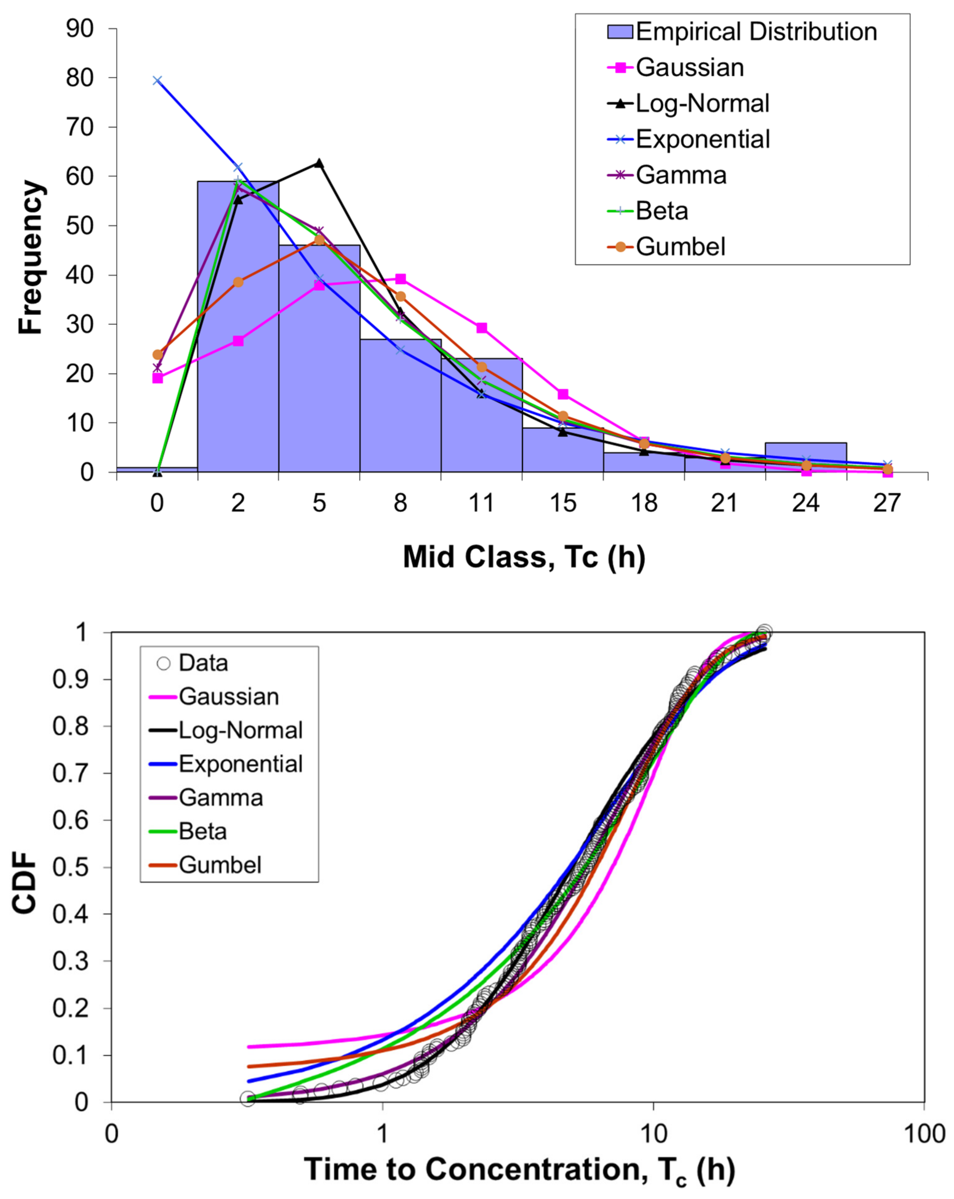
3.3. Probability Distribution and Hypothesis Testing

Figure 6 presents the frequency histogram (6a) and the probability distribution fitting (6b) of the observed Tc data. These distributions, namely Gaussian, log-normal, exponential, Gamma, Beta, and Gumbel distributions, were applied to fit the data. Hypothesis testing was applied to determine which distributions fit the data well.
Accordingly, the KS test at a 5% significant level shows that the log-normal, Gamma, and Beta distributions fit the data well, with KS values of 0.053, 0.052, and 0.095, respectively. Thus, the null hypothesis is accepted for these three distributions. To further determine which of the three fitting distributions is the best distribution, the AIC criterion was applied. AIC values for log-normal, Gamma, and Beta distributions were 449.5, 446.6, and 457.9, respectively. The log-normal distribution, with the lowest AIC value, produced the best distribution to fit the Tc data. This result is useful for quantifying the uncertainty of Tc and, consequently, the uncertainty of peak flow.

4. Conclusions

In evaluating the application of the existing Tc models and their performance in arid regions, the model performance indicators used in this study show that different Tc models perform better regarding some indicators than the others. The following conclusions are derived from our findings:
  • The Dooge model shows the highest correlation with observed Tc at an r equal to 0.60, while the Izzard and Hicks model shows the least correlation at an r equal to −0.15.
  • With regard to the predictive capability, the Jung model shows the best predictive efficiency, with Nash–Sutcliffe efficiency and normalized Nash–Sutcliffe efficiency values of 0.33 and 0.60, respectively, while USGS shows the poorest predictive efficiency, with Nash–Sutcliffe efficiency and normalized Nash–Sutcliffe efficiency values of −550.12 and 0.00, respectively.
  • Based on the mean error and root mean square error, the Jung model produced the least mean error of −0.10 h, while USGS resulted in the largest mean error of 120.77 h. Similarly, the Jung model produced the least root mean square error of 4.72 h, while USGS produced the largest root mean square error of 1643 h.
  • According to the relative bias, the highest underestimation is observed with the Albishi et al. (2017) [19] model at −77%, the least underestimation with the Jung model at −1%, the highest overestimation with USGS at 1643%, and the least overestimation with Kirpich at 4%.
  • It is observed that 80% of all the models evaluated overestimated observed Tc, while the remaining 20% underestimated observed Tc in arid regions.
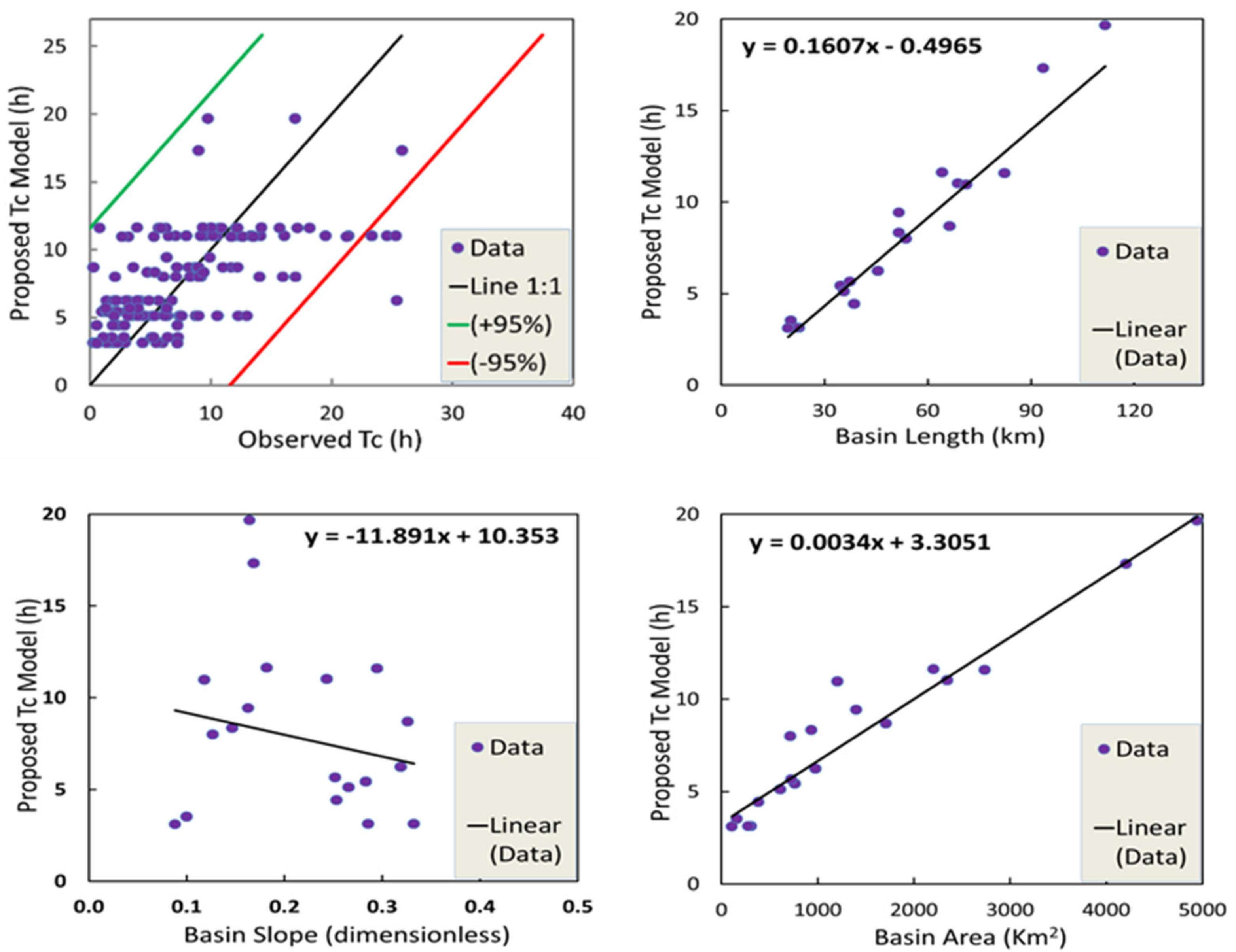
  • The new Tc model developed from data in arid environments performed better than the models evaluated, with a correlation coefficient of 0.62, mean error of 0.07 h, root mean square error of 4.53 h, relative bias of 0.9%, as well as Nash–Sutcliffe efficiency of 0.38 and normalized Nash–Sutcliffe efficiency of 0.62. This proposed model is recommended to be used in flood studies in the Saudi arid environment.
  • Hypothesis testing revealed that log-normal, Gamma, and Beta distributions are a good fit for the Tc data in arid regions at a 5% significance level.
  • The AIC test, which was applied to demonstrate the best probability distribution, shows that log-normal provides the best fit for the observed Tc data at a 5% significance level.

Author Contributions

Conceptualization, A.E. and N.A.; methodology A.E. and K.A.; software, A.E.; validation, A.E., K.A., N.A. and H.E.; formal analysis, N.A., A.E., K.A. and H.E.; investigation, N.A., A.E., K.A. and H.E.; resources, A.E. and K.A.; writing—original draft preparation, K.A.; writing—review and editing, K.A., A.E., N.A. and H.E.; visualization, A.E., H.E. and N.A.; supervision; A.E., H.E. and N.A.; project administration, N.A. and A.E. All authors have read and agreed to the published version of the manuscript.

Funding

This research received no external funding.

Institutional Review Board Statement

Not applicable.

Informed Consent Statement

Not applicable.

Data Availability Statement

Not applicable.

Acknowledgments

The authors appreciate the technical support of the Department of Hydrology and Water Resources Management, Faculty of Meteorology, Environment and Arid Land Agriculture.

Conflicts of Interest

The authors declare no conflict of interest.

References

  1. Kirpich, Z.P. Time of Concentration of Small Agricultural Watersheds. Civ. Eng. 1940, 10, 362. [Google Scholar]
  2. Fang, X.; Cleveland, T.; Garcia, C.A.; Thompson, D.; Malla, R. Literature Review on Timing Parameters for Hydrographs; Department of Civil Engineering, Lamar University: Beaumont, TX, USA, 2005. [Google Scholar]
  3. Johnstone, D.; Cross, W.P. Elements of Applied Hydrology; Ronald Press: New York, NY, USA, 1949. [Google Scholar]
  4. Nagy, E.D.; Torma, P.; Bene, K. Comparing Methods for Computing the Time of Concentration in a Medium-Sized Hungarian Catchment. Slovak J. Civ. Eng. 2016, 24, 8. [Google Scholar] [CrossRef] [Green Version]
  5. Kaufmann de Almeida, I.; Kaufmann Almeida, A.; Garcia Gabas, S.; Alves Sobrinho, T. Performance of Methods for Estimating the Time of Concentration in a Watershed of a Tropical Region. Hydrol. Sci. J. 2017, 62, 2406–2414. [Google Scholar] [CrossRef]
  6. Bengtson, H. Rational Method Hydrologic Calculations with Excel; Continuing Education and Development, Inc.: Woodcliff Lake, NJ, USA, 2011; Volume 942, Available online: https://www.cedengineering.com/userfiles/Rational%20Method%20with%20Excel-R1.pdf (accessed on 11 December 2022).
  7. Hadadin, N. Evaluation of Several Techniques for Estimating Stormwater Runoff in Arid Watersheds. Environ. Earth Sci. 2013, 69, 1773–1782. [Google Scholar] [CrossRef]
  8. Michailidi, E.M.; Antoniadi, S.; Koukouvinos, A.; Bacchi, B.; Efstratiadis, A. Timing the Time of Concentration: Shedding Light on a Paradox. Hydrol. Sci. J. 2018, 63, 721–740. [Google Scholar] [CrossRef] [Green Version]
  9. Saini, A.; Sahu, N.; Kumar, P.; Nayak, S.; Duan, W.; Avtar, R.; Behera, S. Advanced Rainfall Trend Analysis of 117 Years over West Coast Plain and Hill Agro-Climatic Region of India. Atmosphere 2020, 11, 1225. [Google Scholar] [CrossRef]
  10. Sahu, N.; Panda, A.; Nayak, S.; Saini, A.; Mishra, M.; Sayama, T.; Sahu, L.; Duan, W.; Avtar, R.; Behera, S. Impact of Indo-Pacific Climate Variability on High Streamflow Events in Mahanadi River Basin, India. Water 2020, 12, 1952. [Google Scholar] [CrossRef]
  11. McEnroe, B.M.; Young, C.B.; Gamarra Zapata, R.A. Estimation of Watershed Lag Times and Times of Concentration for the Kansas City Area; Bureau of Research, Department of Transportation: Kansas, KS, USA, 2016. [Google Scholar]
  12. Yoo, C.; Lee, J.; Cho, E. Theoretical Evaluation of Concentration Time and Storage Coefficient with Their Application to Major Dam Basins in Korea. Water Supply 2019, 19, 644–652. [Google Scholar] [CrossRef] [Green Version]
  13. Jung, K.; Marpu, P.R.; Ouarda, T.B. Impact of River Network Type on the Time of Concentration. Arab. J. Geosci. 2017, 10, 546. [Google Scholar] [CrossRef]
  14. Perdikaris, J.; Gharabaghi, B.; Rudra, R. Reference Time of Concentration Estimation for Ungauged Catchments. Earth Sci. Res. 2018, 7, 58–73. [Google Scholar] [CrossRef]
  15. Fang, X.; Thompson, D.B.; Cleveland, T.G.; Pradhan, P.; Malla, R. Time of Concentration Estimated Using Watershed Parameters Determined by Automated and Manual Methods. J. Irrig. Drain. Eng. 2008, 134, 202–211. [Google Scholar] [CrossRef]
  16. González-Álvarez, Á.; Molina-Pérez, J.; Meza-Zúñiga, B.; Viloria-Marimón, O.M.; Tesfagiorgis, K.; Mouthón-Bello, J.A. Assessing the Performance of Different Time of Concentration Equations in Urban Ungauged Watersheds: Case Study of Cartagena de Indias, Colombia. Hydrology 2020, 7, 47. [Google Scholar] [CrossRef]
  17. Gericke, O.J.; Smithers, J.C. Review of Methods Used to Estimate Catchment Response Time for the Purpose of Peak Discharge Estimation. Hydrol. Sci. J. 2014, 59, 1935–1971. [Google Scholar] [CrossRef]
  18. Wheater, H.S.; Laurentis, P.; Hamilton, G.S. Design Rainfall Characteristics for South-West Saudi Arabia. Proc. Inst. Civ. Eng. 1989, 87, 517–538. [Google Scholar] [CrossRef]
  19. Albishi, M.; Bahrawi, J.; Elfeki, A. Empirical Equations for Flood Analysis in Arid Zones: The Ari-Zo Model. Arab. J. Geosci. 2017, 10, 51. [Google Scholar]
  20. USDA. National Engineering Handbook, Section 4: Hydrology; USDA: Washington, DC, USA, 1972.
  21. de Almeida, I.K.; Almeida, A.K.; Anache, J.A.A.; Steffen, J.L.; Sobrinho, T.A. Estimation on Time of Concentration of Overland Flow in Watersheds: A Review. Geosci. Geociências 2014, 33, 661–671. [Google Scholar]
  22. Azizian, A. Uncertainty Analysis of Time of Concentration Equations Based on First-Order-Analysis (FOA) Method. Am. J. Eng. Appl. Sci. 2018, 11, 327–341. [Google Scholar] [CrossRef]
  23. Zolghadr, M.; Rafiee, M.R.; Esmaeilmanesh, F.; Fathi, A.; Tripathi, R.P.; Rathnayake, U.; Gunakala, S.R.; Azamathulla, H.M. Computation of Time of Concentration Based on Two-Dimensional Hydraulic Simulation. Water 2022, 14, 3155. [Google Scholar] [CrossRef]
  24. Dooge, J.C.I. Synthetic Unit Hydrographs Based on Triangular Inflow. Ph.D. Thesis, Iowa State University, Ames, IA, USA, 1956; 103p. [Google Scholar]
  25. Clark, C.O. Storage and the Unit Hydrograph. Trans. Am. Soc. Civ. Eng. 1945, 110, 1419–1446. [Google Scholar] [CrossRef]
  26. Nejadhashemi, A.P.; Sheridan, J.M.; Shirmohammadi, A.; Montas, H.J. Hydrograph Separation by Incorporating Climatological Factors: Application to Small Experimental Watersheds 1. JAWRA J. Am. Water Resour. Assoc. 2007, 43, 744–756. [Google Scholar] [CrossRef]
  27. Farran, M.M.H. Statistical Analysis of SCS-CN Curve Number for Improved Estimation of Flash Floods in Arid Regions: Case Study in the Southwest of Saudi Arabia. Master’s Thesis, King Abdulaziz University, Jeddah, Saudi Arabia, 2020. [Google Scholar]
  28. Kolmogorov, A. Sulla Determinazione Empirica Di Una Lgge Di Distribuzione. Inst. Ital. Attuari Giorn. 1933, 4, 83–91. [Google Scholar]
  29. Smirnov, N.V. Estimate of Deviation between Empirical Distribution Functions in Two Independent Samples. Bull. Mosc. Univ. 1939, 2, 3–16. [Google Scholar]
  30. Laio, F.; Di Baldassarre, G.; Montanari, A. Model Selection Techniques for the Frequency Analysis of Hydrological Extremes. Water Resour. Res. 2009, 45, W07416. [Google Scholar] [CrossRef]
  31. Kite, G.W. Frequency and Risk Analysis in Hydrology; Water Resources: Fort Collins, CO, USA, 1978. [Google Scholar]
Figure 1. Illustration of the graphical definition of time of concentration, Tc: the time from the centroid of effective rainfall to the inflection point on the recession limb of the total runoff hydrograph.
Sustainability 15 01987 g001
Figure 2. Map of the study area showing the major drainage basins and their sub-watersheds. The colors show the DEM = digital elevation model.
Sustainability 15 01987 g002
Figure 3. Observed rainfall hyetographs and corresponding direct runoff hydrographs in the study watersheds. Obs. Hydrograph = observed hydrograph.
Sustainability 15 01987 g003
Figure 4. Comparison between Tc models and observed Tc in the study area: the black line is a line of the perfect fit, the green line is the +95% upper bound, and the red line is the −95% lower bound.
Sustainability 15 01987 g004
Figure 5. Scatterplot of the proposed Tc model versus observed Tc (topleft), basin length (topright), basin slope (bottomleft), and basin area (bottomright) in the study area.
Sustainability 15 01987 g005
Figure 6. (Top) Frequency histogram, and (bottom) fitting probability distribution function of Tc with the different theoretical frequency distributions.
Sustainability 15 01987 g006
Table 1. Summary of geomorphological, rainfall, and runoff parameters of the study area.
ParameterDefinitionRange
Basin Area, A (km2)-107–4.944
Basin Slope, Sb (m/m)The average slope of the entire basin0.09–0.33
Basin length, Lb (km)Length in a straight line from the mouth of a stream to the farthest point on the drainage divide of its basin19–112
Basin elevation, Hm (m)Difference between the elevation of the highest basin divide and the elevation at the basin outlet234.72–2143.95
Flow length, L (km)Downslope distance from the hydraulically most distant point to the outlet point26–158
Flow length slope, S (m/m)Mean steepness, i.e., the ratio between the mean fall and the L length of the basin’s hydraulically most distant points0.01–0.08
Average rainfall intensity, i (mm/h)-0.19–41.13
Roughness coefficient, n-0.04
Curve number, CN-44–98
Runoff coefficient, C-0.0014–0.3724
Table 2. List of models selected for the estimation of Tc.
S/NModelEquation for TcDefinition of Parameters
1Kirpich (1940) [1] T c = 0.0663 S 0.385 L 0.77 Tc (h) = time of concentration; L (km) = main water line length; and S (m/m) = mean channel slope
2Soil Conservation Service Lag (1972) [20] T c = 0.057 1000 C N 9 0.7 L 0.8 S 0.5 Tc (h) = time of concentration; CN: SCS curve number; L (km) = flow path length; S (m/m) = mean slope of channel
3Federal Aviation Administration (1970) [21] T c = 0.3788 1.1 C L 0.5 S 0.333 Tc (h) = time of concentration; C: runoff coefficient; L (km) = length of flow path; S (m/m) = mean channel slope
4Carter (1961) [21] T c = 0.0977 L 0.6 S 0.2 Tc (h) = concentration time; L (km) = main water line length; S (m/m) = mean channel slope/mean steepness
5Kinematic Wave Formula (1964) [21] T c = 7.35 L 0.6 n 0.6 i 0.4 S 0.2 Tc (h) = concentration time; L (km) = length of the main water line or flow path length; S (m/m) = mean slope of channel/mean steepness; n = Manning’s roughness coefficient; i (mm/h) = rainfall intensity
6Jung (2005) [12] T c = 0.119   ( L 0.777 S 0.212 )Tc (h) = concentration time; L (km) = channel length; S = channel slope
7Espey (1966) [22] T c = 6.89   L S 0.36 Tc (h) = concentration time; L (km) = channel length; S = slope of basin or channel slope
8Kraven I (1999) [12] T c = 0.0074   L S 0.515 Tc (h) = concentration time; L (km) = channel length; S = slope of basin or channel slope
9United States Geological Survey (2000) [12] T c = 1.54   ( L 0.875 S 0.181 )Tc (h) = concentration time; L (km) = channel length; S = slope of basin or channel slope
10Ven Te Chow (1962) [23] T c = 0.1602 L 0.64   S 0.32 Tc (h) = time of concentration; L (km) = main water line length or flow path length; and S (m/m) = average channel steepness
11United States Army Corps of Engineers (1954) [4] T c = 0.191 L 0.76   S 0.19 Tc (h) = time of concentration; L (km) = length of the main water line or flow path length; and S (m/m) = average channel steepness
12.Albishi et al. (2017) [19] T c = L 0.09 S 0.11 Tc (h) = time of concentration; L (km) = basin length; and S (m/m) = average basin slope
13Morgali and Linsley (1965) [22] T c = 7.354   n 0.6 L 0.6 S 0.3 i 0.4 Tc (h) = time of concentration; L (km) = main water line length; S (m/m) = mean channel slope/mean steepness; n = Manning’s roughness coefficient; i (mm/h) = rainfall intensity
14Izzard and Hicks (1946) [8] T c = 3.46   0.0007 i + C L 0.33 S 0.333 i 0.667 Tc (h) = time of concentration; L (km) = channel length; S (m/m) = basin/channel slope; n = Manning’s roughness coefficient; i = in/h
15McCuen et al. (1984) [22] T c = 2.2535 i 0.7164   L 0.5552 S 0.207 Tc (h) = time of concentration; L (km) = main water line length; S (m/m) = mean channel slope/mean steepness; i (mm/h) = rainfall intensity
16Johnstone (1949) [5] T c = 0.4623 L 0.5   S 0.25 Tc (h) = time of concentration; L (km) = main water line length; S (m/m) = mean channel slope/mean channel steepness; i (mm/h) = rainfall intensity
17Dooge (1973) [24] T c = 0.365 A 0.41   S 0.17 Tc (h) = time of concentration; S (m/m) = mean channel slope/mean channel steepness; A (km2) = area of the basin
18Giandotti (1934) [8] T c =     4 A + 3 2 L 0.8 H m Tc (h) = time of concentration; L (km) = main water line length; A (km2) = area of the basin; Hm (m) = mean altitude in the basin (i.e., mean elevation starting from the mouth)
19Haktanir and Sezen (1990) [4] T c = 0.7473 L 0.841 Tc (h) = time of concentration; L (km) = main water line length
20Sheridan (1994) [17] T c = 2.20 L 0.92 Tc (h) = time of concentration; L (km) = main water line length
Table 3. PDFs used in the study.
Distribution TypePDF FormulaParameters of PDF
µσ2
Gaussian f X = 1 β 2 Π e 1 2 β 2 X α 2       < X < αβ2
Log-normal f X = 1 X β 2 Π e 1 2 β 2 L n X α 2       X > 0 αβ2
Exponential f X = 1 α e α X           α > 0 , X > 0 1 α 1 α 2
Gamma f X = 1 β α Γ α X α 1 e X β       α , β > 0 , X > 0 α β α β 2
Beta f X = Γ α + Γ β Γ α Γ β X α 1 1 X β 1       α , β > 0 , X > 0 α α + β αβ/(α + β)2 (α + β + 1)
Gumbel f X = 1 β e X α β e X α β   < X < α + 0.5772β Π 2 6   β 2
µ = mean; σ2 = variance of the distribution.
Table 4. Performance indicators and indices.
Tc ModelMean Model Tc (h)Mean Observed Tc (h)rME (h)PBIAS (%)RMSE (h)NSENNSEData Outbound ±95% Confidence Limits (%)
Kirpich (1940) [1]7.647.350.570.2944.830.300.591.9
SCS Lag (1972) [20]22.947.350.3615.5921221.54−12.920.072.5
FAA (1970) [21]11.357.350.574.00546.40−0.230.450
Carter (1961) [21]2.627.350.58−4.73−647.06−0.500.4046
Kinematic Wave (1964) [21]19.147.350.4911.7916015.68−6.380.121.9
Jung (2005) [12]7.257.350.58−0.10−14.720.330.603.1
Espey (1966) [22]60.917.350.5753.5672955.36−91.000.010.6
Kraven I (1999) [12]3.957.350.56−3.40−465.89−0.040.4913
USGS (2000) [12]128.127.350.58120.771643135.5−550.120.001.9
Ven Te Chow (1962) [23]8.117.350.570.76104.810.300.591.9
USACE (1954) [4]9.927.350.582.58355.510.090.520
Albishi et al. (2017) [19]1.667.350.52−5.69−778.07−0.960.3467.7
Morgali and Linsley (1965) [22]28.257.350.5020.9028426.59−20.220.042.5
Izzard and Hicks (1946) [8]9.487.35−0.152.132917.15−7.830.103.1
McCuen et al. (1984) [22]31.177.350.3923.8232434.10−33.900.032.5
Johnstone (1949) [5]9.737.350.572.38325.300.160.540
Dooge (1973) [24]11.847.350.604.49616.55−0.290.440
Giandotti (1934) [8]9.017.350.581.66235.070.230.560.6
Haktanir and Sezen (1990) [4]26.837.350.5719.4826521.56−12.960.070
Sheridan (1994) [17]111.607.350.57104.251419114.61−393.310.001.2
Proposed Tc Model7.427.350.620.070.94.530.380.623.1
Disclaimer/Publisher’s Note: The statements, opinions and data contained in all publications are solely those of the individual author(s) and contributor(s) and not of MDPI and/or the editor(s). MDPI and/or the editor(s) disclaim responsibility for any injury to people or property resulting from any ideas, methods, instructions or products referred to in the content.

