Comprehensive Thermodynamic Performance Evaluation of Various Gas Liquefaction Cycles for Cryogenic Energy Storage

Abstract

This paper conducts comparative thermodynamic analysis and performance evaluations of various gas liquefaction configurations. The four most common liquefaction systems (Linde–Hampson, Kapitza, Heylandt, and Claude) were considered. The isothermal and multi-stage isentropic compression processes were evaluated and compared as actual compression processes. Thermodynamic evaluation is based on the energy required to compress a unit mass of gas, the liquefied air mass flow rate, and the exergetic efficiency. The modeling results show that three-stage compression cycles retain lower energy requirements. Increasing the compression stage from one to two for all the processes decreases the energy requirement by 34 to 38%. Changing the compression stage number from two to three reduces the energy requirement by 13%. The compression pressure and expander flow rate ratio significantly affect the liquefied air mass flow rate. Hence, a parametric analysis was conducted to obtain the best operating conditions for each considered cycle. Depending on the compression pressure, the optimum expander flow rate values of the Claude, Kapitza, and Heylandt cycles change from 0.65 to 0.5, 0.65 to 0.55, and 0.35 to 0.30, respectively. For the optimum cases, the Claude, Kapitza, and Heylandt cycles result in liquid yields that are about 2.5, 2.2, and 1.6 times higher than that of the Linde–Hampson cycle. The Claude cycle is the best operating cycle for all the considered performance metrics. Moreover, the performances of the Linde–Hampson and Claude cycles are investigated for various gases. Under the same operating conditions, the results show that better performance parameters are obtained with the gases that have relatively high normal boiling temperatures.

1. Introduction

Cryogenics, which deals with the production, storage, and utilization of cryogen, is an engineering technology that is applied to very low-temperature refrigeration applications, such as those in the liquefaction of gases and the study of physical phenomena at temperatures under 123 K and close to absolute zero [1]. Rapid advancements in many scientific domains are made possible by cryogenic technologies, including superconductivity in physics, cryogenic synthesis in chemistry, long-term storage of biological cells in biology, cryogenic electron microscopy in analytic sciences, and calibration in instrumentation. Cryogenic technology is also widely used for medical applications; for instance, liquid nitrogen is used to protect blood, tissue, etc., for an extended time [2]. Cryogenic fluids can be kept for many months in low-pressure insulated storage tanks with minimum loss [3]. There is a comprehensive application of cryogenic technology, including the liquefaction of various industrial gases, such as nitrogen [4], oxygen [5], helium, hydrogen [6], natural gas [7], etc. Liquefied natural gas (LNG) has gained popularity in the energy sector as a means of storing natural gas on a large scale and transporting it hundreds of miles from the locations of production to cities and nations [8,9]. It is expected that liquid hydrogen will undergo activities that are comparable to those of the development of the hydrogen economy concept [10,11]. Liquid hydrogen has commonly been used as a fuel for space vehicles. Another application is cryogenic food processing, which uses liquid nitrogen as the refrigerant for preserving food. As many critical scientific and engineering processes require cryogenic fluids, the liquefaction of gases is an important research topic for researchers and engineers.

Due to the intermittent nature of renewable energy supply systems, energy storage has gained critical importance, and different energy storage technologies have emerged. There are various technologies for storing electricity. Batteries are a competitive solution due to their fast response to short-duration storage up to 4 h [12,13]. However, large-scale battery storage is uncommon because of low energy densities, small power capacities, and short cycle life [14]. They are not economically feasible for medium- to long-duration storage. In terms of large-scale energy storage systems, pumped hydroelectric, compressed air, and cryogenic energy storage systems (CES) are commercially available [14].

CES has gained attention due to its high energy density and because it is geographically unconstrained. CES is based on the liquefaction of ambient air at −196 °C, reducing its specific volume by around 700 times [15]. Liquefied air can be stored in unpressurized tanks for many months. When needed, the liquid air is pumped, evaporated, and heated with a higher temperature source, then expanded in turbines to generate electricity [16]. Liquid air does not require large storage volumes compared to other energy storage technologies [17]. The response time is around 2.5 min for CES systems, which is much faster than the compressed air storage system (CAES) of 8–12 min [15,18]. Liquid gases are a potential sustainable energy vector for many applications. The liquefied gases have a much higher energy density (150–250 Wh/kg) compared to the compressed gas form (30–60 Wh/kg) [15]. In comparison, lead-acid batteries have an energy density of 30 Wh/kg, and Li-ion batteries have an energy density of 120–183 Wh/kg [19].

The main working principle of CES is simple, and it has three main subsystems: charging, storing, and discharging. During the charging cycle of the system, electricity or renewable power is used to compress air to high pressure [20]. The process can be utilized in one or multiple stages [21]. Between the compression stages, the air is cooled in heat exchangers. Finally, the air is expanded by expanders such as cryo-turbines or a Joule–Thompson valve and stored in a tank. In the discharge process, the liquefied gas is pumped to supercritical pressure, then evaporated and superheated; afterwards, the high-pressure gas is expanded by a series of expanders utilizing a part of the electricity charged to the system. The liquefaction process of the system is energy-intensive, which is the main drawback of this system.

Primary air liquefaction cycles have been used commercially for more than a century since Carl Linde patented his cycle [22,23]. However, the first research on the topic of CES was published in 1974, and this technology has become popular only in recent years [24]. The Linde–Hampson, Claude, Kapitza, and Heylandt cycles are the most commonly used air liquefaction cycles. Compared to other energy storage technologies, the CES system is a relatively new technology that must be investigated thoroughly. The key parameters that influence the performance of the liquefaction process are the liquefaction cycle used, the heat exchanger effectiveness, the efficiency of the compressors and the turbines, the charging pressure, etc. [25]. In recent years, much research has been conducted to enhance CES conversion efficiency, which can be achieved by improving system configuration, optimizing thermal storage capabilities, and integrating the system with external heat sources [26].

Yilmaz et al. [27] investigated the thermodynamic performances of liquefaction cycles such as the simple Linde–Hampson, precooled Claude, and precooled Kapitza cycles using an isothermal compression process. The performance metrics for the study are the liquefaction fractions, performance coefficients, and second law efficiencies of the cycles. The results show that the precooled Claude and Kapitza cycles perform better than the Linde–Hampson cycle. Borri et al. [28] conducted a comparative parametric analysis for various air liquefaction cycles. The liquefaction plant aims to produce 10 tons of liquefied air per day. The results of the study showed that the Kapitza and Claude cycles with multi-stage compression had lower specific energy consumption than the Linde–Hampson cycle.

Researchers commonly use the round-trip efficiency (RTE) of gas liquefaction systems as a basis for comparison. The RTE can be defined as the ratio between the electricity charged and the electricity discharged. The RTE of the CES systems is usually between 45 and 60% [15]. Dzido et al. [20] investigated the unit energy expenditures and the round-trip efficiency of the six typical air liquefaction cycles. The authors investigated various cases; among them, the highest efficiency of 57.72% was obtained for the Kapitza cycle at a 100 bar regasification pressure. She et al. [29] investigated the performance of a CES system from a heat transfer and energy storage perspective. The study results showed that the liquid air storage tank efficiency strongly affects the round-trip efficiency of the CES system. Therefore, it is recommended to pay attention to the thermal insulation of the tanks.

CES systems can also be integrated with other technologies to increase round-trip efficiency. Tafone et al. [30] investigated the techno-economic feasibility analysis of the integration of the organic Rankine cycle (ORC) for waste heat recovery in CES systems. The results of the study showed that integrating the ORC into LAES systems decreases the levelized storage cost and is, therefore, economically feasible. In another study, Tafone et al. [24] investigated the potential improvement of the round-trip efficiency of CES systems with the implementation of the ORC and an absorption chiller. The performance of the CES system with the ORC and absorption chiller integration was investigated under full electric and trigenerative modes. The authors showed that integrating ORC systems into the CES systems can improve the round-trip efficiency by up to 20%. The integration of the absorption chiller decreases the energy requirement by the CES systems; however, the round-trip efficiency is not improved significantly. Xue et al. [31] proposed a novel combined cooling, heating, and power system based on the CES. The proposed system configuration included an ORC to recover high-temperature compression heat to utilize electricity. In addition, an absorption refrigeration system was also used for low-temperature compression heat for district cooling. The results of the study showed that the RTE could reach up to 69.64%, which is 37.66% higher than the baseline CES system.

Although the gas liquefaction systems have gained the attention of many researchers, their potential under realistic operating conditions has not yet been wholly demonstrated [24]. The literature review shows that the research regarding gas liquefaction systems still needs improvement. The liquefaction section of the CES system is vital, and proper design can significantly increase efficiency. The high specific energy consumption during the liquefaction process is the main drawback that adversely influences system efficiency. Therefore, the system needs to be designed with minimum specific energy consumption. In particular, there needs to be a detailed comparison between various configurations of gas liquefaction systems under different operating conditions with more realistic approaches. There is a lack of studies in this field that investigate the performance enhancement of these systems comparatively. In addition, many previous studies considered the compression to be an isothermal process. In this study, isothermal, isentropic, and actual compression processes were all considered. In this context, the main contributions and the novelty of the present study could be stated as follows:

-

The mathematical models for the liquefaction systems are coded in the Engineering Equation Solver (EES) environment [31], and the set of equations is solved in an iterative manner by the EES software. The thermodynamic properties of the real fluids are obtained by using the EES internal libraries.

-

The most common gas liquefaction systems are compared with both isothermal and real (one, two, and three stages) compression processes for the liquefaction of air and some of the frequently used gases.

-

A wide range of compression pressures from 3 MPa to 20 MPa is considered in the assessment of the liquefaction performances.

-

A wide range of the expander flow rate from 0.15 to 0.8 is considered in the assessment of the liquefaction performances for the Claude, Kapitza, and Heylandt cycles.

-

The comparative evaluation of the performances of various gas liquefaction systems is performed by considering the coefficient of performance (COP), the figure of merit (FOM) (or exergy efficiency), the specific energy consumption, and the liquefied air yield under different operating conditions.

-

The influence of the compressor intake air temperature on the liquid yield of the Linde-based and the Claude-based cycles was also investigated.

2. System Description

Various cycles can be used for gas liquefaction. This study investigated the Linde–Hampson, Claude, Kapitza, and Heylandt cycles under both isothermal and real compression. In isothermal compression, heat is removed during the compression process by an external cooling fluid. However, the compression process, in reality, occurs with irreversibility. Therefore, it is assumed that the actual compression process with irreversibility can be predicted by using isentropic efficiency. Isentropic efficiencies for the compressors and turbines were defined with the help of the literature data for actual processes. An after-cooler removes the heat from the compressed gas for each compression stage. This study considers and compares one-stage, two-stage, and three-stage compression configurations.

2.1. Linde–Hampson Cycle

A simple Linde–Hampson cycle is the system with the most basic configuration. However, it is not the easiest one to operate due to high operation pressures. Also, the liquid yield of this cycle is low. The system consists of a compressor, an after-cooler, a heat exchanger, a phase separator, and a Joule–Thompson (J-T) valve. The schematic of the simple Linde–Hampson system and the T-s diagram are presented in Figure 1. (1–2) Air at atmospheric pressure and temperature (27 °C and 101 kPa) is mixed with the uncondensed portion of the gas from the previous cycle and compressed by the compressor and exits at state 2 s when the isentropic compression is assumed; it exits at state 2 when the actual compression occurs. It should be highlighted that many researchers previously modeled this stage as isothermal compression. However, modeling the compression stage as isothermal is unrealistic. Therefore, an after-cooler is used to reject the heat after the compression stage (2–3). After passing the after-cooler, the air is further cooled with the uncondensed portion of gas from the previous cycle (3–4). Cooled air expands in a Joule–Thompson (J-T) valve, resulting in a two-phase fluid (4–5). Liquefied air (8) is separated and stored, and the gas portion of the mixture (7) is sent back to the system.

In real applications, no process can be completely isentropic. To compare the actual compression, isentropic efficiency can be used. The isentropic efficiency (${\eta }_{Comp}$) and compression ratio (CR) of the air compressor can be given as Equations (1) and (2), respectively.

$${\eta }_{Comp}=\frac{h_{2s}-h_1}{h_2-h_1}$$

(1)

In Equation (1), $h_{2s}$ is the specific enthalpy for the isentropic case, whereas $h_2$ is the specific enthalpy for the actual case at the compressor exit.

$$CR=\frac{P_2}{P_1}$$

(2)

Then, the actual compression work, W_act, is obtained from Equation (3) [32].

$$W_{act}=\frac{h_2-h_1}{{\eta }_c}=\frac{kR{T}_1}{{\eta }_c(k-1)}\left[{\left(CR\right)}^{\frac{k-1}{k}}-1\right]$$

(3)

where R is the gas constant, and k is the specific heat ratio.

It should be noted that the Joule–Thomson throttling process is isenthalpic; so, the energy balance at the Joule–Thomson valve can be written as:

$$h_4=h_5$$

(4)

2.2. Claude Cycle

The Claude cycle and its modifications are commonly used in commercial air liquefaction plants due to their higher efficiency compared to the Linde cycle [33]. Most of the potential work might be destroyed due to irreversibilities during the isenthalpic expansion process. Therefore, the utilization of both isenthalpic and isentropic expansion processes can be applied to increase the refrigeration effect. The Claude cycle uses both a J-T valve and an isentropic expander. In Figure 2, the schematic and the T-s diagram for the Claude cycle are presented. In the Claude cycle, the air is compressed (1–2 s for the isentropic process and for 1–2 for the actual process) and passed through the after-cooler (2–3). The air is further cooled at the HX1 (3–4). Between 0.15 and 0.75 portions of the air are diverted from the mainstream and expanded at the turbine (14–15 s for the isentropic process and 14–15 for the actual process). This diverted portion of the air returns the stream at the second mixer (M2); then, the mixed stream enters the HX3. The expander flow rate ratio (efr) is a parameter of the study.

In real applications, no process can be completely isentropic. To compare the actual expansion process in the expander, isentropic efficiency can be used. The isentropic efficiency (${\eta }_{exp}$) of the expander can be given as Equation (5).

$${\eta }_{exp}=\frac{h_{15}-h_{14}}{h_{15s}-h_{14}}$$

(5)

In Equation (5), $h_{15s}$ is the specific enthalpy for the isentropic case, whereas $h_{15}$ is the specific enthalpy for the actual case at the expander exit.

2.3. Kapitza Cycle

The Kapitza cycle is a modified version of the Claude cycle. The only difference is that HX3 is removed from the system. The isentropic efficiency of the expander is taken as 0.7 for the Kapitza, Heylandt, and Claude cycles. The overall system configuration and the T-s diagram are presented in Figure 3.

2.4. Heylandt Cycle

The Heylandt cycle is one of the most common air liquefaction systems; it is a variant of the Claude cycle. In this cycle, the HX1 in the Claude cycle is eliminated. A portion of the air enters the expander directly. In Figure 4, the schematic and T-s diagram of the Heylandt system are presented.

3. Performance Indicators and Validation

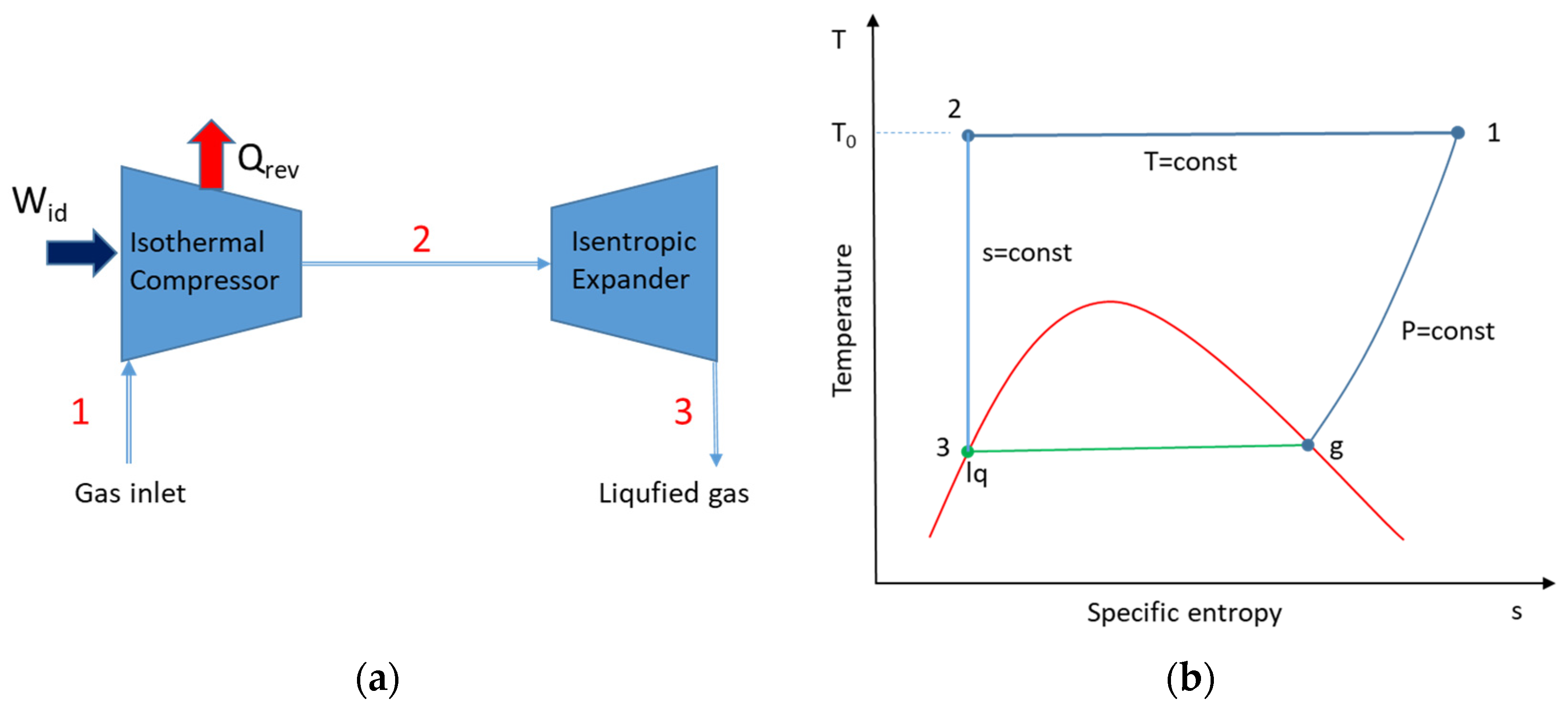
It is necessary to develop an appropriate reference system to compare the performances of different liquefaction cycles. The thermodynamically perfect system characterizes the physical bounds of a process. Therefore, the Carnot refrigeration cycle is typically used as a reference. Liquefaction, on the other hand, is essentially an open-system configuration. As a result, the ideal liquefaction system simply requires the first two steps in the Carnot cycle: reversible isothermal compression followed by reversible adiabatic (isentropic) expansion to the saturated liquid state. Figure 5 shows the schematics of the ideal system and the temperature–entropy variation diagram.

Applying the first and second laws of thermodynamics around the whole system, the following expression, Equation (6), can be obtained for the ideal work, which is equal to the minimum work requirement for the liquefaction of a gas [2]:

$$-\frac{W_{id}}{m_{comp}}=T_0\left(s_0-s_{lq}\right)-\left(h_0-h_{lq}\right)$$

(6)

where m_comp is the mass flow rate of the gas; T₀ is the ambient temperature; s_lq and h_lq are the specific entropy and enthalpy of the liquefied gas, respectively; and s₀ and h₀ are the specific entropy and enthalpy of the gas, respectively, at ambient conditions. As all the gas entering the compressor is liquefied, the cooling effect (Q_lq) could be expressed as given in Equation (7).

$$\frac{Q_{lq}}{m_{comp}}=\left(h_0-h_{lq}\right)$$

(7)

The coefficient performance (COP_id) of the ideal system could be obtained by the ratio of the cooling effect to the required ideal work, as given in Equation (8).

$${COP}_{id}=\frac{Q_{lq}}{W_{id}}$$

(8)

In contrast to the ideal liquefaction process, it is only possible to liquefy some of the gas entered into the compressor for the real liquefaction systems. Therefore, the liquid yield, y, is defined as the ratio of the mass of liquid gas produced (m_lq) to the mass of air compressed (m_comp) by the compressor in the system. The liquid yield is a key performance indicator in any plant involving gas liquefaction. Liquid yield can be presented as given in Equation (9) [34]:

$$y=\frac{m_{lq}}{m_{comp}}$$

(9)

In addition to that, the minimum compression work for the real liquefaction cycles, such as the Linde–Hampton, Claude, etc., is expressed by using reversible isothermal compression between the states 1 and 3 (shown in Figure 1, Figure 2, Figure 3 and Figure 4) with constant T, as given in Equation (10).

$$-\frac{W_{isoth}}{m_{comp}}=T_1\left(s_1-s_3\right)-\left(h_1-h_3\right)$$

(10)

Considering the irreversibilities in the compressor, the compression work could be calculated as given in Equation (11).

$$-\frac{W_{isoth}}{m_{comp}}=\frac{T_1\left(s_1-s_3\right)-\left(h_1-h_3\right)}{{\eta }_{comp}}$$

(11)

where η_comp is the isothermal efficiency of the compressor.

For refrigeration systems, the figure of merit (FOM) is explained as the ratio of the ideal (reversible) system’s COP_id to the actual system’s COP_act. In this definition, the FOM is also equal to the exergetic efficiency of the refrigerator. According to the definition of the FOM, it can be obtained by using Equation (12) for a liquefaction system.

$$FOM=\frac{{COP}_{act}}{{COP}_{id}}=\frac{{y W}_{id}}{W_{act}}$$

(12)

where W_id and W_act represent the ideal and the real power consumptions, respectively.

One of the critical parameters used to compare the performances of various gas liquefaction cycles under the same conditions is the specific energy consumption per unit of liquid produced (SEC_lq). SEC_lq (kWh/t or kJ/kg) can be given as follows [28]:

$${SEC}_{lq}=\frac{W_{net}}{m_{lq}}$$

(13)

In Equation (13), m_lq is the mass flow rate of the liquefied air to the total compressed air flow rate in the cycle. W_net is the net energy requirement for air liquefaction, which can be found as given below:

$$W_{net}=\sum W_{comp}-W_{exp}$$

(14)

In Equation (14), W_comp and W_exp are the power consumption of the compressor and the expander.

The performance of the Claude-based cycles is dependent on the expander flow rate ratio (efr) [19]. The expander flow rate ratio can be defined as the mass flow rate through the expander (m_exp) over the mass flow rate through the last compression step (m_comp) [19]:

$$efr=\frac{m_{exp}}{m_{comp}}$$

(15)

The optimum expander flow rate ratio is investigated for the Claude, Kapitza, and Heylandt cycles.

The mathematical models for the liquefaction systems are coded in the Engineering Equation Solver (EES, Version 11) [35], and the set of equations is solved in an iterative manner by the EES software. The thermodynamic properties of the real fluids are obtained by using the EES internal libraries. As the cryogenic energy storage systems have been in the development stage, there are only a few pilot plants in the testing stage. Therefore, the validation of the present liquefaction models is performed by using the numerical studies reported by Kanoğlu et al. [36], Borri et al. [28], and Hamdy et al. [33]. 

Table 1. Comparisons of performance parameters of a simple Linde–Hampson cycle for various gases.

Gases	NBP (K)	y		SECiso (kJ/kg)		COPiso		COPid		FOM
		Present	Ref. [36]	Present	Ref. [36]	Present	Ref. [36]	Present	Ref. [36]	Present	Ref. [36]
Air	78.9	0.082	0.082	5500	5481	0.077	0.077	0.579	0.578	0.133	0.134
Nitrogen	77.35	0.076	0.076	6197	6193	0.070	0.070	0.566	0.566	0.123	0.123
Oxygen	90.19	0.107	0.107	3826	3755	0.106	0.108	0.643	0.644	0.165	0.168
Argon	87.3	0.122	0.122	2697	2650	0.101	0.103	0.577	0.576	0.175	0.178
Methane	111.7	0.199	0.199	4111	3889	0.221	0.234	0.842	0.843	0.263	0.278
Fluorine	85.03	0.077	0.077	4508	4459	0.076	0.077	0.609	0.609	0.125	0.127

compares the present calculation results and the data obtained from the reference [36]. The operating conditions of a simple Linde–Hampson cycle were taken as defined in the reference. It can be seen that the present mathematical model results showed a good agreement with the corresponding results from the works of Kanoğlu et al.

In

Table 2. Comparison of the results of the present study to the other studies.

Process	Working Conditions	SEC (kJ/kg)		y		FOM		Ref.
		Present	Ref.	Present	Ref.	Present	Ref.
Claude	P2 = 4 MPa, Tamb = 300 K ηcomp = 0.85, ηexp = 0.85, efr = 0.5	4618	5040	0.110	0.105	0.160	0.158	[28]
Kapitza	P2 = 4 MPa, Tamb = 300 K ηcomp = 0.85, ηexp = 0.85, efr = 0.4	4204	4140	0.140	0.145	0.176	0.179	[28]
Claude	P2 = 20 MPa, Tamb = 288 K, T3 = 298 K ηcomp = 0.87, ηexp = 0.80, efr = 0.5	2229	2206	0.319	0.307	0.314	0.317	[33]
Kapitza	P2 = 20 MPa, Tamb = 288 K, T3 = 298 K ηcomp = 0.87, ηexp = 0.80, efr = 0.4	2260	2210	0.308	0.306	0.310	0.317	[33]
Heylandt	P2 = 20 MPa, Tamb = 288 K, T3 = 298 K ηcomp = 0.87, ηexp = 0.80, efr = 0.4	2325	2299	0.289	0.288	0.301	0.304	[33]

, the comparison between the present model calculations and the data obtained from the reference studies were given for the Claude, Kapitza, and Heylandt cycles. The studies of Borri et al. [28] and Hamdy et al. [33] were used for the comparisons. When the working conditions of the selected studies are considered, the results of the present models are in good agreement with the literature data. As a result of this, the current mathematical models and the calculation procedures are accepted as validated.

4. Results and Discussion

The main assumptions that are taken into account throughout the modeling are as follows:

• Gas enters the system at atmospheric pressure and temperature;
• The after-cooler outlet temperature is the atmospheric temperature;
• The cycles are modeled in steady flow conditions;
• The isentropic efficiency of the compressor is set to 0.85;
• The isentropic efficiency of the expander is set to 0.70;
• The gas mass flow rate at state 1 is one kg/s;
• The auxiliary electrical losses and heat losses to the environment are neglected.

The optimum working conditions are determined by employing parameters, namely atmospheric pressure and temperature, compression pressure, and recirculation fraction (efr for Claude, Kapitza, and Heylandt cycles). The compression unit in each cycle is modeled as isothermal compression with internal cooling and an isentropic compressor with an after-cooler. One, two, and three stages of isentropic compression with an after-cooler are considered for the compression unit. Three scenarios (one, two, or three compression stages) corresponding to four different liquefaction cycles (Linde–Hampson, Kapitza, Claude, and Heylandt) were assessed. The main results are given in the following sections.

4.1. Performance of Linde–Hampson Cycle

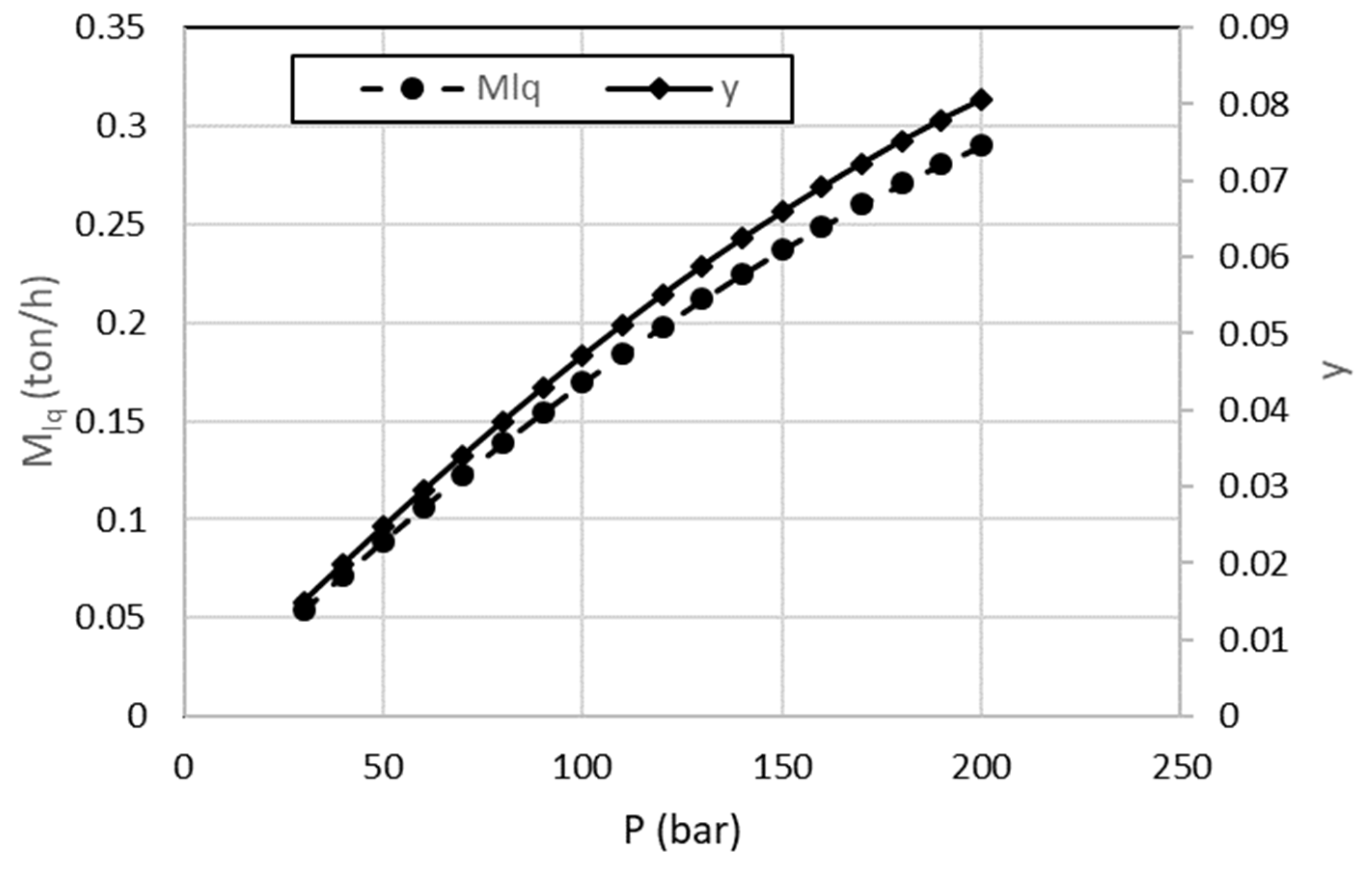
The first liquefaction configuration considered in this study is the Linde–Hampson system. The liquefied air mass flow rate and the liquid yield depend on the compression pressure. Figure 6 shows the relation between the compression pressure, the liquefied mass flow rate, and the liquid yield. For different pressures, the y value for the Linde–Hampson cycle changes from 0.01 to 0.09, which is compatible with the literature results [22,27,33]. As the compression pressure increases, the liquid air yield also increases. For a 200 bar compression pressure, m_lq is 0.2902 ton/h, and the liquid yield is 0.080. By decreasing the liquefaction pressure from 200 to 40 bar, the liquid yield and the liquefied mass flow rate are reduced by 75%.

Increasing the compression stage number is beneficial, as the compression process becomes similar to the isothermal compression. To decrease the compression work, the same cycle is also modeled with two and three compression stages. During the actual compression process, the gas being compressed does not occur at the constant temperature that it does in the isothermal process. To make comparisons, the system with isothermal compression is considered a thermodynamically ideal system, and it was also analyzed. The results of the specific work requirement of the various cases are presented in Figure 7. An increase in the compression pressure results in a significant reduction in the specific energy consumption for all the processes. As can be seen from the results, modeling the compressor isothermally significantly decreases energy consumption. Depending on the pressure, the SEC_lq value is between 43 and 57% lower for the Linde–Hampson cycle with isothermal compression compared to the same system with one-stage isentropic compression. The difference is more significant for high pressures. The SEC_lq value is between 24 and 35% lower and 19 and 25% lower for the cycle with isothermal compression, compared to two-stage and three-stage isentropic compression, respectively.

The lowest SEC_lq value of 1842 kWh/ton can be achieved at 200 bar for isothermal compression, and it is followed by the three-stage compression system; when the compression stage number increases, the system becomes similar to the isothermal compression. The results are compatible with the literature data [28].

The FOM of a refrigeration system is equal to the exergetic efficiency. Figure 8 gives the FOM values for the Linde–Hampson cycle with one, two, and three compression stage configurations and the isothermal compression. For the cycle with isothermal compression at 40 bar pressure, the FOM value is 43.13% greater than the same cycle with one-stage isentropic compression and 24.35% and 16.86% greater than the cycle with two- and three-stage isentropic compression, respectively. At 200 bar pressure, the process with isothermal compression has 56.58%, 34.14%, and 24.25% higher FOM values than the cycles with one-stage, two-stage, and three-stage isentropic compression. The cycle with an isothermal compression at 200 bar pressure has the most significant FOM value of 0.1117, followed by the three-stage compression cycle with a 0.0846 value.

4.2. Performance of Claude Cycle

The Kapitza, Heylandt, and Claude cycles use both the isenthalpic and isentropic expansion processes to increase the refrigeration effect. Therefore, the Kapitza, Heylandt, and Claude cycles have one expander and one expansion valve. In Figure 9, the liquefied mass flow rate versus the compression pressure and the expander flow rate ratio are given for the Claude cycle. At higher pressures, greater liquefied mass flow rate values can be obtained. From 40 to 200 bar, the liquid yield increases by 68.34%. The liquefied air mass flow rate increases with the expander flow rate ratio for a specific value and becomes the maximum. After that optimum value, it starts to decrease. Each respective pressure has an optimum expander flow ratio. For instance, the maximum liquefied air flow rate of 0.7096 ton/h can be obtained at 20 MPa and a 0.55 efr value. For 4 MPa compression pressure, the maximum liquefied air mass flow rate of 0.3873 ton/h can be produced at a 0.65 efr value.

In Figure 10, the specific energy consumption of the Claude cycle with isothermal compression and the actual compression with one, two, and three compression stages is given, with varying compression pressure and efr values. The specific energy consumption is minimal at the optimum efr value of each respective pressure. At 20 MPa and a 0.55 efr value, the specific work is 678.2 kWh/ton for the system with isothermal compression. It can be seen from the results that when the number of compression stages is increased, the compression process becomes nearly isothermal; therefore, the compression work decreases. The system with three-stage compression, at 20 MPa and a 0.55 efr value, has an 894.5 kWh/ton energy requirement. The system with one- and two-stage compression at the same pressure and efr has 1660 kWh/ton, and 1040 kWh/ton, respectively. Therefore, it can be concluded that the system with isothermal compression has a 59% lower specific energy requirement than the system with one-stage compression and a 36% and 26% lower specific energy requirement than the system with two-stage and three-stage isentropic compression, respectively.

Figure 11a shows the FOM values for the Claude cycle with isothermal compression versus e_fr and compression pressures. The results reveal that the maximum FOM value of 0.3034 can be obtained at 20 MPa, and a 0.55 efr value. The maximum FOM value of each compression pressure can be obtained at the optimum efr value of the respective pressure.

Figure 11 also presents the FOM values for the Claude cycle with one (b), two (c), and three (d) compression stages, respectively. The results highlight the fact that the FOM values highly depend on compression pressure, efr values, and the compression stage number. For the cycle with actual compression, the highest FOM value of 0.23 can be obtained at 20 MPa compression pressure, a 0.55 efr value, and three compression stages.

4.3. Performance of Kapitza Cycle

For the Kapitza cycle, a specific amount of gas is diverted into the expander after the compression process to produce work. The remaining flow share enters the HX2 and the throttling valve. This diverted stream (expander flow rate) influences the system’s performance. To understand the influence of the expander flow rate ratio (efr) and the compression pressure on the liquefied air mass flow rate, the efr varies from 0.15 to 0.80. The compression pressure ranged from 40 to 200 bar. The results are presented in Figure 12. Each compression pressure has its optimum efr value that gives the maximum liquefied air mass flow rate. For instance, at 20 MPa, the 0.5 efr value has the highest m_lq value of 0.6681 ton/h. At 4 MPa, the 0.65 efr value has the highest liquefied mass flow rate of 0.3384 ton/h. Therefore, the optimum efr values change according to the compression pressures. For a constant efr value of 0.60, changing the pressure from 40 to 200 bar increases the liquefied mass flow rate by 93.66%.

The influence of both the pressure and the expander flow ratio on the specific work requirement of the Kapitza cycle with isothermal compression is given in Figure 13a. At high compression pressures, the optimum expander flow ratio values are lower. At 20 MPa, the 0.5 efr value has the lowest specific energy requirement of 609.7 kWh/ton. In comparison, at 4 MPa, the 0.65 efr value is the optimum, providing the lowest SEC value of 1006 kWh/ton at this pressure. Therefore, it is recommended to use the optimum expander flow ratio values for the respective pressure to achieve the lowest specific energy consumption and the highest liquefied air mass flow rate.

Figure 13 gives specific energy consumption results for the Kapitza cycle with one-stage (b), two-stage (c), and three-stage (d) actual compression, respectively. The results show that the specific energy consumption is much higher for all the cases than for the cycle modeled with isothermal compression. Optimum efr values of each respective pressure can also be obtained from the figures. For the 0.5 efr value and 20 MPa compression pressure, the one-, two-, and three-stage cycles have the SEC values of 1766 kWh/ton, 1158 kWh/ton, and 998 kWh/ton, respectively. The same process with isothermal compression has 65%, 36%, and 26% lower specific energy consumption compared to the cycle with one-, two-, and three-stage isentropic cycles, respectively.

Figure 14a presents the FOM values for the Kapitza cycle with isothermal compression. The results reveal that the maximum exergetic efficiency of 0.3339 can be obtained at 20 MPa and a 0.5 efr value. It can be concluded that, in terms of the specific energy requirement, maximum liquefied mass flow rate, and exergetic efficiency, selecting the optimum expander flow ratio at the respective compression pressure is crucial. Figure 14 also presents the FOM values for the cycles with one-stage (b), two-stage (c), and three-stage (d) compression. Among all the investigated cases for actual compression, the cycle with three compression stages, at 20 MPa pressure and a 0.5 efr value, has the highest FOM value of 0.2062.

4.4. Performance of Heylandt Cycle

As one of the most commonly used air liquefaction systems, the Heylandt system is another variant of the Claude cycle. In Figure 15, the liquefied mass flow rate values are shown for the Heylandt cycle with varying efr values and compression pressure. The results highlight that the maximum liquefied mass flow rate can be achieved at higher compression pressures. In comparison to the Kapitza and Claude cycles, for each respective pressure, lower expander flow rate ratio values give higher liquefied air mass flow rate values. The Heylandt cycle reaches the maximum liquefied air mass flow rate value of 0.4821 ton/h, at 20 MPa and a 0.3 efr value.

Figure 16a shows the specific energy consumption for the Heylandt system with isothermal compression. The results reveal that as with the previous cycles, the specific consumption reduces with increasing pressure. The lowest energy consumption of 1009 kWh/ton can be obtained at 20 MPa and a 0.35 efr value. Figure 16b–d present the specific energy consumption of the Heylandt cycle modeled with one-, two-, and three-stage actual compression, respectively. Among all the investigated cases, the system with one-stage compression has the highest energy consumption. When the compression stage increases, the energy requirement for the air liquefaction can be decreased. For the three-stage compression, the lowest energy requirement value of 1341 kWh/ton can be obtained at 20 MPa compression pressure and a 0.35 efr value. The system with isothermal compression at the same operating conditions has 26%, 36%, and 59% lower specific energy requirements than the cycle with three-stage, two-stage, and one-stage isentropic compression, respectively.

In terms of exergetic efficiency, the FOM values for the Heylandt cycle with isothermal compression and one-, two-, and three-stage actual compression cases were presented in Figure 17a–d, respectively. The results of the study revealed that the maximum FOM value could be obtained by the isothermal compression case with a 0.204 value at 20 MPa compression pressure and a 0.35 efr value. The cycle with the three-stage compression, at the same pressure and efr value, has a 0.1534 FOM value. For the two-stage and one-stage compression, at the same pressure and efr value, the FOM values are 0.132 and 0.08, respectively.

4.5. Comparison of the Optimum Cycles

In Figure 18, all the cycles with optimum operating parameters were compared with regard to specific energy consumption. The results show that the systems with isothermal compression have the lowest energy requirement. Among the systems with actual compression, the Claude cycle with three compression stages has the lowest SEC_lq value, and it is closely followed by the Kapitza cycle with three stages. The two-stage Claude and Kapitza cycles come next. After the Claude and Kapitza cycles, the Heylandt cycle performs best with regard to specific energy consumption. With regard to specific energy consumption, the Linde–Hampson cycle is the most energy-intensive cycle. The single-stage Linde–Hampson cycle has the most significant energy requirement of 4243 kWh/ton, even at the optimum conditions. For all the cycles, increasing the compression stage from one to two decreases the energy requirement by 34 to 38%. Changing the compression stage number from two to three decreases the energy requirement by 13%.

In Figure 19, the liquid yield values are compared for all the cycles. As can be seen, the liquid yield is the greatest for the Claude cycle with a value of 0.1971, followed by the Kapitza cycle with a 0.1856 value. The Heylandt cycle has a 0.1339 liquid yield. The Linde–Hampson cycle has the lowest liquid yield with a 0.08 y value. The Linde–Hampson cycle has 60%, 56.5%, and 40% lower liquid yields than the Claude, Kapitza, and Heylandt cycles, respectively.

In Figure 20, the comparison of all the cycles at optimum operating parameters was presented with regard to exergetic efficiency. The Claude cycle with three compression stages has the highest FOM value of 0.23, followed by the Kapitza cycle with 0.2062. The Claude cycle and Kapitza cycle with two-stage compression come after that. The three- and two-stage Heylandt cycle tracks them. The results show that the Linde–Hampson cycle has low exergetic efficiencies. The Linde–Hampson cycle with single-stage compression has a FOM value of 0.048.

The cycles working with different gases have different performances due to differences in the thermo-physical properties of the gases. As a result, a parametric study is conducted for the Linde–Hampson and Claude cycles with optimum design parameters. The results for the Linde–Hampson cycle are presented in

Table 3. Performance parameters of a Linde–Hampson cycle for various gases.

Gases	NBP (K)	y	Mlq (ton/h)	SECact (kWh/ton)	SECiso	COPact	COPiso	COPid	FOMact	FOMiso
Air	78.9	0.081	0.290	2432	1842	0.049	0.064	0.576	0.085	0.112
Nitrogen	77.4	0.074	0.266	2752	2087	0.044	0.058	0.563	0.078	0.103
Oxygen	90.2	0.105	0.378	1667	1261	0.068	0.089	0.639	0.106	0.140
Argon	87.3	0.119	0.43	1321	889.1	0.058	0.085	0.573	0.100	0.149
Methane	111.7	0.195	0.702	1669	1308	0.152	0.194	0.836	0.182	0.232
Fluorine	85.0	0.075	0.27	1931	1498	0.050	0.064	0.605	0.082	0.106
CO	81.6	0.084	0.304	2407	1821	0.051	0.068	0.586	0.088	0.116

. It can be seen that different refrigerants have different liquid yields, liquid mass flow rates, specific energy consumption, COP, and FOM values. The most excellent liquid yield can be produced for the cycle with methane gas with a 0.195 value, and the argon gas follows it with a 0.119 value. Nitrogen can produce the least amount of liquid yield. The results also show that the amount of the liquid yield is related to the boiling temperature, as the refrigerant with a higher boiling temperature has a greater liquid yield. Regarding SEC, argon is the most favorable refrigerant, as the SEC value is 1321 kWh/ton. The least favorable refrigerant is nitrogen, with 2752 kWh/ton. In terms of COP and FOM values, methane is the best-performing refrigerant. The liquid yield is between 38 and 62% lower for the other gases compared to methane.

In

Table 4. Performance parameters of a Claude cycle for various gases.

Gases	NBP (K)	y	Mlq (ton/h)	SECact (kWh/ton)	SECiso	COPact	COPiso	COPid	FOMact	FOMiso
Air	78.9	0.197	0.711	923	682	0.128	0.174	0.576	0.223	0.302
Nitrogen	77.4	0.192	0.691	986	730	0.122	0.165	0.563	0.217	0.293
Oxygen	90.2	0.218	0.785	744	549	0.152	0.206	0.639	0.238	0.322
Argon	87.3	0.233	0.839	640	419	0.119	0.181	0.573	0.207	0.317
Methane	111.7	0.286	1.029	1057	810	0.240	0.314	0.836	0.288	0.375
Fluorine	85.0	0.193	0.694	692	524	0.139	0.183	0.605	0.229	0.303
CO	81.6	0.2	0.720	944	697	0.131	0.177	0.586	0.223	0.302

, the results are presented for the Claude cycle with various refrigerants. Regarding the liquid yield, methane has the most excellent y value with 0.286. Argon has a 0.233 liquid yield, which is 18% lower than methane. Oxygen has a 0.218 liquid yield value that is 23% lower than methane. Nitrogen can produce the least liquefied gas with a 0.192 y value, which is 33% lower than methane.

Regarding the specific energy consumption, the cycle with methane as the refrigerant is the most energy-intensive. The system with argon as the refrigerant is the most favorable with regard to energy consumption. Regarding COP_act and the FOM_act, the system with methane as the refrigerant performs the best.

4.6. The Effect of Gas Inlet Temperature on the Linde-Based and Claude-Based Cycles

To understand the influence of the compressor intake temperature on the system performance of the Linde-based cycles, the input air temperature is varied from 10 to 45 °C, and the liquid fraction and the specific energy consumption are investigated. The results are given in Figure 21. It can be concluded that when the intake temperature increases, the liquid fraction decreases, and the specific consumption increases sharply. From a 10 to 45 °C intake temperature, the liquid yield decreases by 30.2%, and the SEC increases by 59%, respectively.

For the Claude-based cycles, a similar trend is observed when the compressor intake temperature is varied. Based on the results given in Figure 22, the liquid yield decreases by 10% when the inlet temperatures increase from 10 to 45 °C. The specific energy consumption increases by 22%. Therefore, it can be highlighted that for both the Claude-based and the Linde-based cycles, increasing the compressor intake temperature has a negative impact as it decreases the liquid yield and increases the energy consumption.

5. Conclusions

Energy storage systems are essential for the sustainable application of renewable energy systems. Among them, liquefied gas systems are particularly important due to their various benefits. In this study, different gas liquefaction systems were modeled, and their performance was assessed and compared. The Linde–Hampson, Claude, Kapitza, and Heylandt liquefaction cycles were modeled. In addition to the actual compression with one, two, and three stages, the isothermal compression case was also investigated. The main parameters for performance evaluation are specific energy consumption, the liquefied air flow rate, liquid yield, and the exergetic efficiency at different operating conditions and configurations. The main findings of the study are summarized below:

Among all the investigated cases, the Linde–Hampson cycle has the highest specific energy consumption and the lowest liquid yield. The liquid yield of the Linde–Hampson cycle is between 0.01 and 0.09. The Claude, Kapitza, and Heylandt cycles have about 2.5, 2.2, and 1.6 times higher liquid yields than the Linde–Hampson cycle, respectively.

For all the cycles, increasing the compression pressure increases the liquid yield and decreases the specific energy consumption.

The cases with isothermal compression have much lower energy requirements for all cycles. Depending on the pressure, the specific energy requirement value is between 43 and 57% lower for the Linde–Hampson cycle with isothermal compression compared to the same system with one-stage isentropic compression. The difference is more significant for high pressures. The SEC value is between 24 and 35% and 19 and 25% lower than the two-stage and three-stage isentropic compression.

For all the cycles, increasing the compression stage from one to two decreases the energy requirement by 34 to 38%. Changing the compression stage number from two to three reduces the energy requirement by 13%.

For the Kapitza, Claude, and Heylandt cycles, the expander flow rate ratio is one of the most critical parameters affecting the performance of the cycle. This parameter is highly dependent on the compression pressure. Therefore, optimum efr values were obtained for each respective pressure. Considering the pressure values between 4 MPa and 20 MPa, the optimum efr values of the Claude, Kapitza, and Heylandt cycles change from 0.65 to 0.5, 0.65 to 0.55, and 0.35 to 0.30, respectively.

The liquid yield highly depends on the compression pressure and efr values. Among all the investigated cycles, the Claude cycle is the best one in terms of the liquid yield. The liquid yield is between 0.10 and 0.21 for 40–200 bar compression pressures for the Claude cycle with the optimum efr value. The liquid yield is between 0.09 and 0.19 for the Kapitza cycle and 0.04 and 0.14 for the Heylandt cycle with the optimum efr value, respectively.

The results of this study show that the optimum plant configuration and operating conditions decrease the specific energy consumption and increase the liquefied air flow rate and the exergetic efficiency. Regarding all the considered performance metrics, the Claude cycle is the best operating cycle.

To understand the influence of the intake air temperature on the liquid yield for the Linde-based and Claude-based cycles, a parametrical analysis was conducted. From a 10 to 45 °C intake temperature, the liquid yield decreases by 30.2%, and 10% and the SEC_lq increases by 59%, and 22% for the Linde-based and Claude-based cycles, respectively.

Due to the differences in thermo-physical properties, the liquefaction systems working with different gases have different performances. The results show that the amount of the liquid yield is related to the boiling temperature, as the refrigerant with a higher boiling temperature has a greater liquid yield. The results show that in terms of liquid yield, COP, and FOM, methane is the best operating fluid for both the Linde–Hampson and Claude cycles. For the Linde–Hampson cycle, the liquid yield is between 38 and 62% lower for the other gases compared to methane. In terms of specific energy consumption, argon has the lowest value among the considered gases.

A future study will investigate the techno-economic performance of the investigated cycles.