


A Study of Population Aging and Urban–Rural Residents’ Consumption Habits from a Spatial Spillover Perspective: Evidence from China

Abstract
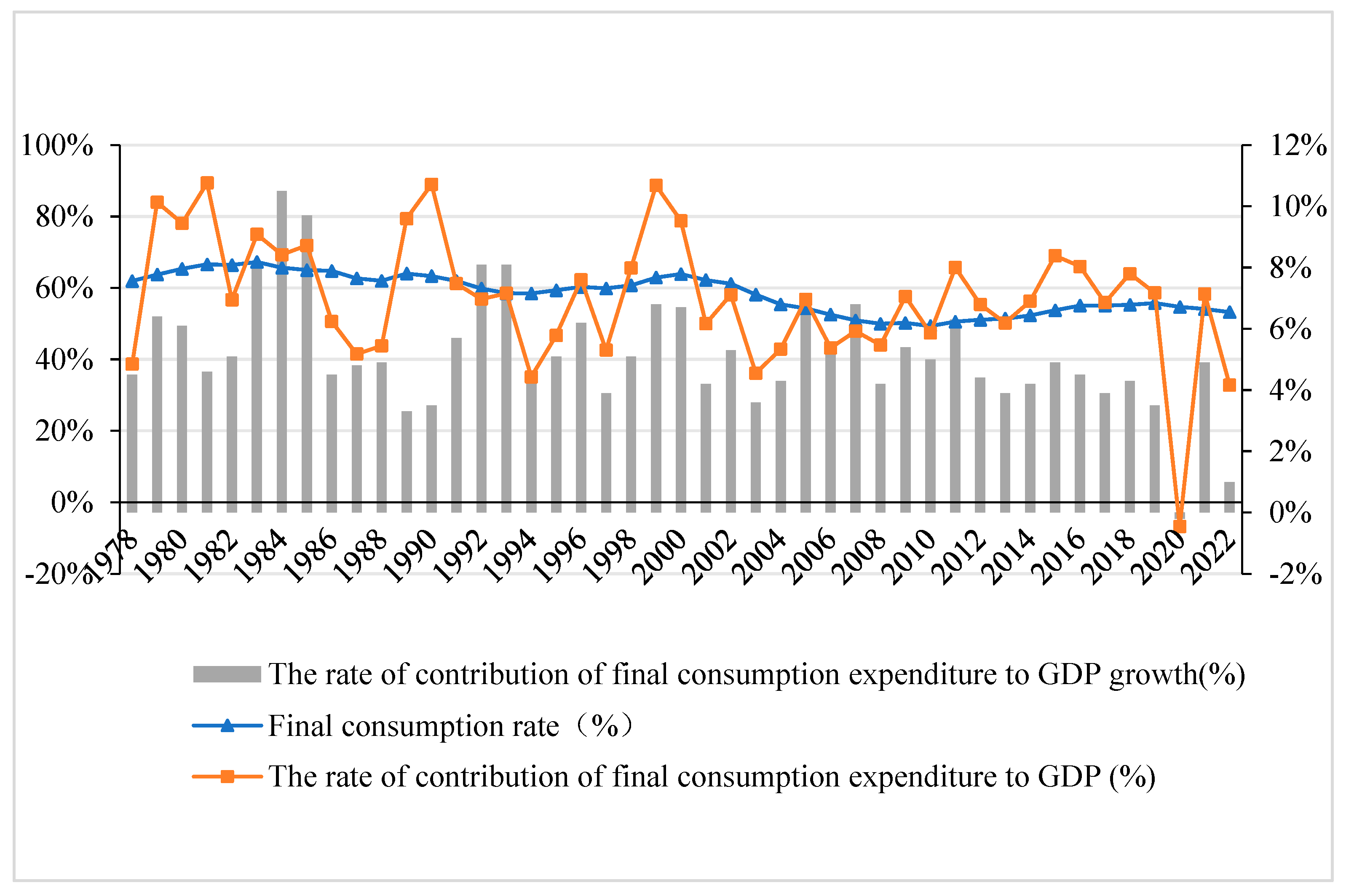
:1. Introduction
2. Literature Review
3. Method
3.1. Construction of Econometric Models
3.2. Variable Selection and Description
3.2.1. Variable Selection
3.2.2. Data Sources and Data Processing
3.2.3. Descriptive Statistics
4. Empirical Results and Analysis
4.1. Spatial Autocorrelation Test for the Main Variables
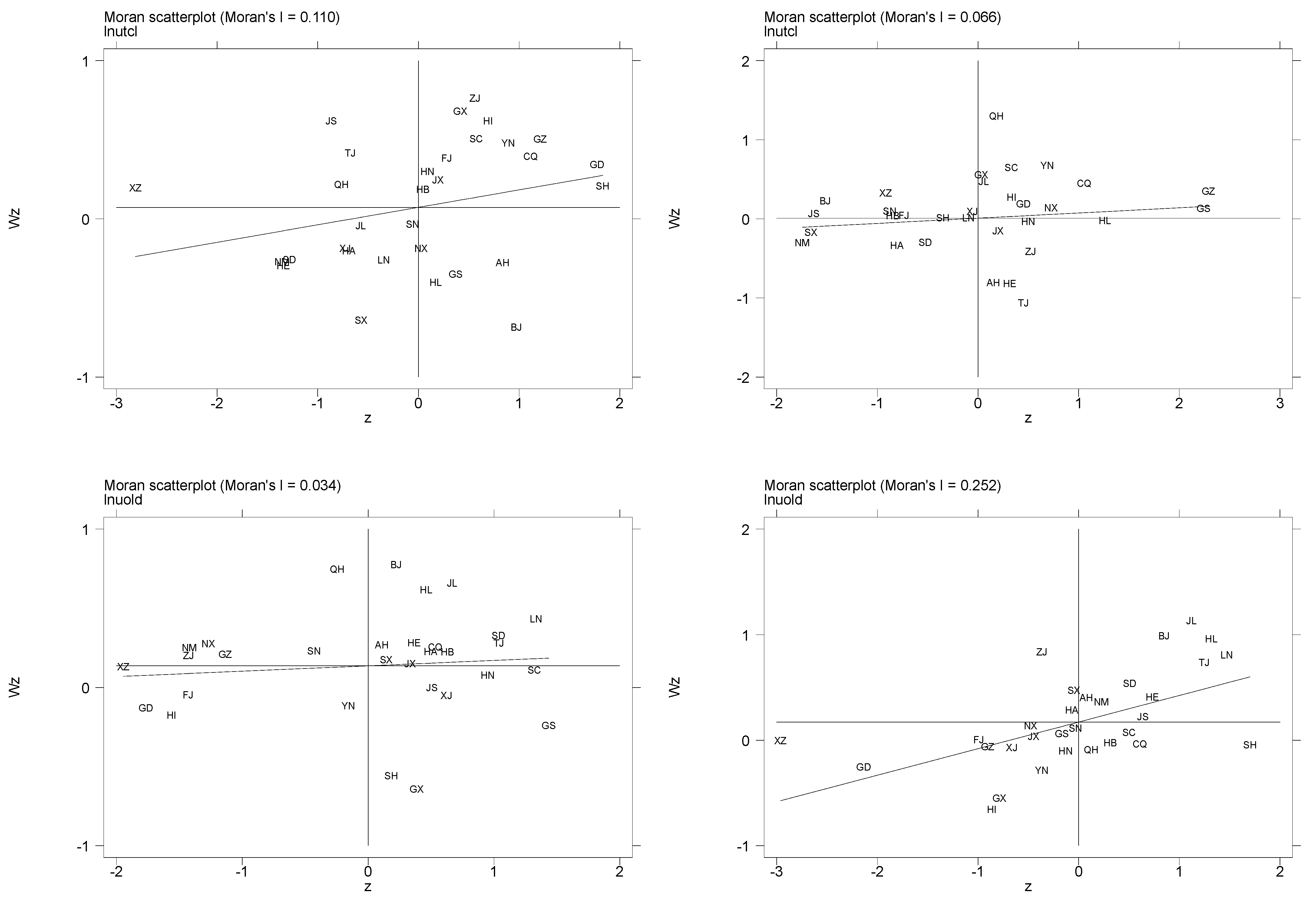
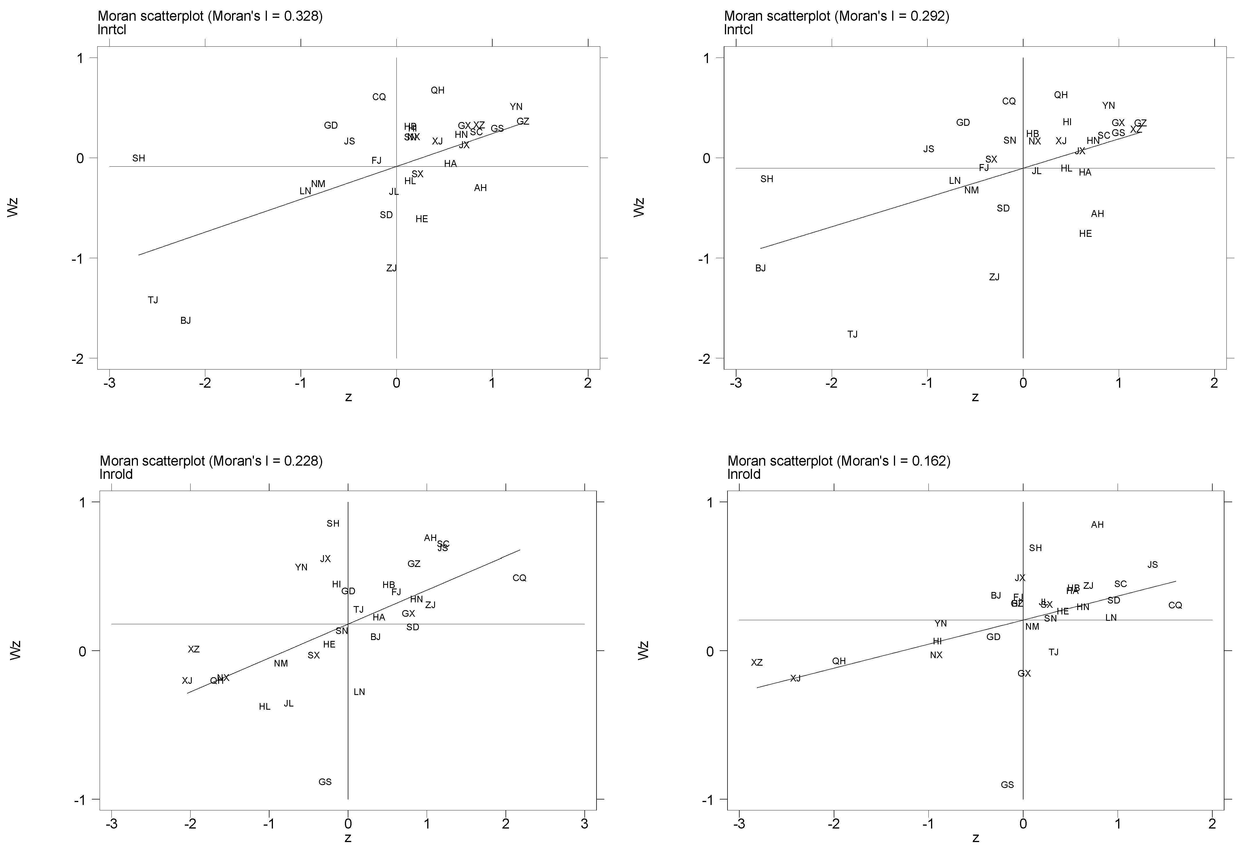
4.1.1. Global Moran’s I
4.1.2. Local Moran’s I
4.2. Selection Test for the SLM and SEM Models
4.3. Analysis of the Empirical Results
4.3.1. Test of the Effect of Population Aging on Narrowing the Consumption Gap between Urban and Rural Residents
4.3.2. Test of the Spatial Effect of Population Aging on the Consumption Levels of Urban and Rural Residents
4.4. Robustness Tests
5. Conclusions, Policy Recommendations, Shortcomings, and Prospects
5.1. Conclusions
5.2. Policy Recommendations
5.3. Shortcomings and Prospects
Author Contributions
Funding
Institutional Review Board Statement
Informed Consent Statement
Data Availability Statement
Acknowledgments
Conflicts of Interest
References
- National Bureau of Statistics of China. Major Figures on 2020 Population Census of China. Available online: http://www.stats.gov.cn/sj/pcsj/rkpc/d7c/ (accessed on 26 November 2021).
- National Bureau of Statistics of China. China Population and Employment Statistical Yearbook. 2022. Available online: https://data.cnki.net/yearBook/single?id=N2023030104 (accessed on 1 December 2022).
- Ren, Z. China Aging Research Report. Available online: https://finance.sina.com.cn/zl/china/2023-02-07/zl-imyewiyr5155477.shtml (accessed on 7 February 2023).
- Huang, W.; Ren, C.; Zhou, Y. Retirement Policies, Labor Supply and Income-Consumption Dynamics. Econo. Res. J. 2023, 58, 141–157. [Google Scholar]
- Central People’s Government. Supporting the Third Pillar of Pension Insurance. Available online: https://www.gov.cn/xinwen/2021-01/11/content_5578690.htm (accessed on 11 January 2021).
- General Office of the Central Committee of the Communist Party of China; General Office of the State Council. Opinions on Promoting the Construction of Basic Elderly Care Service System. Available online: https://www.gov.cn/zhengce/202305/content_6875434.htm (accessed on 21 May 2023).
- CPC Central Committee. Suggestions on Formulating the 14th Five Year Plan for National Economic and Social Development and the Long Range Goals for 2035. Available online: http://www.mofcom.gov.cn/article/zt_sjjwzqh/fuzhu/202012/20201203021505.shtml (accessed on 4 November 2020).
- Xi, J. Report to the 20th National Congress of the CPC. Available online: http://www.qstheory.cn/yaowen/2022-10/25/c_1129079926.htm (accessed on 25 October 2022).
- Wu, Y.; Chen, Z. Spatial Correlation and Regional Convergence Analysis of Residents’ Consumption Levels. World Econ. Pap. 2009, 5, 76–89. [Google Scholar]
- Yin, X.; Sun, H. Resident Consumption, Spatial Dependence and Conditional Convergence—A Research Based on Spatial Panel Data. Chin. Econ. Stud. 2011, 4, 47–59. [Google Scholar]
- Shi, M.; Liu, X. Space, Consumption Stickiness and the Low Consumption Ratio Puzzle. J. Renmin Univ. China 2015, 3, 46–56. [Google Scholar]
- National Development and Reform Commission of China. Measures to restore and expand consumption. Available online: https://www.gov.cn/zhengce/content/202307/content_6895599.htm (accessed on 31 July 2023).
- Modigliani, F.; Brumberg, R. Utility Analysis and the Consumption Function: An Interpretation of Cross-section Data. J. Post Keynes Econ. 1954, 01, 388–436. [Google Scholar]
- Liu, Z.; Song, Z. The Retirement Consumption Puzzle: Evidence from China Urban Household. Chin. J. Popul. Sci. 2013, 13, 94–103. [Google Scholar]
- Modigliani, F.; Cao, S.L. The Chinese Saving Puzzle and the Life Cycle Hypothesis. J. Econ. Lit. 2004, 42, 145–170. [Google Scholar] [CrossRef]
- Wang, J.; Fu, X. Taking into Account Changes in the Age Structure of the Population Econometric Analysis of Consumption Function in China—Also Discusses the Impact of Aging Chinese on Consumption. Popul. Res. 2006, 1, 29–36. [Google Scholar]
- Li, C.; Zhang, J. The Effect of the Transformation of Chinese Population Structure on the Consumption of the Rural Residents. Chin. J. Popul. Sci. 2009, 4, 14–22. [Google Scholar]
- Mao, Z.; Sun, W.; Hong, T. Comparative Analysis on the Relationship between Population Age Structure and Household Consumption in China. Popul. Res. 2013, 3, 82–92. [Google Scholar]
- Li, X.; Wang, C.; Lv, M. Structure of Population Age and Consumption of Rural Residents Theoretical Mechanism and Empirical Inspection. Jianghai Acad. J. 2010, 2, 93–98. [Google Scholar]
- Zhang, L.; Lei, L. An Analysis of the Relation of the Regional Population Age Structure and the Household Consumption in China. Popul. Econ. 2011, 1, 16–21. [Google Scholar]
- Fan, Z.; Zhou, S. The impact of urbanization, population age structure on residents’ consumption and regional differences. Cons. Econ. 2016, 4, 21–25. [Google Scholar]
- Sheng, L.; Fang, X.; Feng, Y.; Liu, H. Study on the Impact of Changes in Household Population Composition on Household Consumption: An Analysis Based on Micro Household Panel Data. Stat. Res. 2021, 11, 35–46. [Google Scholar]
- Tu, Q. A Study on the Threshold Effect of Population Aging on Urban Residents’ Consumption. J. Com. Econ. 2018, 18, 36–39. [Google Scholar]
- Pan, H.; Tang, Y. Research on the Impact of Population Aging on Residents’ Consumption Rate. Jiangxi Soc. Sci. 2021, 1, 51–60. [Google Scholar]
- Leff, N.H. Dependency rates and savings rates. Am. Econ. Rev. 1969, 59, 886–896. [Google Scholar]
- Horioka, C.Y. A Cointegration Analysis of the Impact of the Age Structure of the Population on the Household Saving Rate in Japan. Rev. Econ. Stat. 1997, 79, 511–516. [Google Scholar] [CrossRef]
- Higgins, M. Demography, National savings, and International Capital Flows. Int. Econ. Rev. 1998, 39, 343–369. [Google Scholar] [CrossRef]
- Ram, R. Dependency Rates and Aggregate Savings: A New International Cross-section Study. Am. Econ. Rev. 1982, 72, 537–544. [Google Scholar]
- Bloom, D.E.; Canning, D.; Bryan, G. Longevity and Life-cycle Savings. Scand. J. Econ. 2003, 105, 319–338. [Google Scholar] [CrossRef]
- Bloom, D.E.; Canning, D.; Mansfield, R.K.; Moore, M. Demographic Change Social Security Systems, and Savings. J. Monet. Econ. 2007, 54, 92–114. [Google Scholar] [CrossRef] [PubMed]
- Schultz, T.P. Demographic Determinants of Savings: Estimating and Interpreting the Aggregate Association in Asia. Chin. Econ. Quart. 2005, 7, 991–1017. [Google Scholar] [CrossRef]
- Wang, Y. A Study on the Impact of Population Aging on the Consumption Behavior of Urban Residents in China. Chin. J. Popul. Sci. 2011, 1, 64–73. [Google Scholar]
- Huang, Y.; Zhang, C.; Tian, S. The Influencing Mechanisms of Population Age Structure and Housing Price on Household Consumption in Urban China. Popul. Res. 2019, 4, 17–35. [Google Scholar]
- Tan, J.; Yang, Y. Population Outflow, Aging and Rural Household Consumption. Popul. J. 2012, 6, 9–15. [Google Scholar]
- Yi, X.; Jian, Q. An Empirical Study on Population Aging and Household Average Propensity of Consumption in China. Cons. Econ. 2019, 2, 3–12. [Google Scholar]
- Yu, X.; Sun, M. A Study of the Impact of the Aging of Population in China on Consumption. Jilin Univ. J. 2012, 1, 141–147. [Google Scholar]
- Ni, H.; Li, S.; He, J. Impacts of Demographic Structure Change on Economic Structure in China: An Analysis Based on Input-Output Model. Stud. Lab. Econ. 2014, 3, 63–76. [Google Scholar]
- Xu, G.; Liu, L. Statistical Testing of China’s Aging Population and Residents’ Consumption Structure. Stat. Dec. 2016, 1, 91–94. [Google Scholar]
- Shi, B. An Empirical Research of Elderly Consumption in Urban and Rural China: With Analysis of “Retirement-Consumption Puzzle”. Popul. Res. 2017, 3, 53–64. [Google Scholar]
- Shi, M.; Jiang, Z.; Qiu, X. How Aging Effects Household Consumption—Evidences from China household Survey Data. Econ. Theory Bus. Manag. 2019, 4, 62–79. [Google Scholar]
- Wang, W.; Liu, Y. Population Aging and Upgrading of Household Consumption Structure—An Empirical Study Based on CFPS2012 Data. J. Shandong Univ. Philo. Soc. Sci. 2017, 5, 84–92. [Google Scholar]
- Wang, J. Research on the Influence of Population Aging on the Consumption Disparity of Chinese Rural and Urban Residents—Based on the Empirical Analysis of Provincial Dynamic Panel Data. Mod. Econ. Sci. 2015, 37, 109–115. [Google Scholar]
- Wang, J.; Zhao, K. Urbanization, Aging, Urban-Rural Gap and Economic Development in China—A Moderated Mediation Model. Cont. Econ. Manag. 2020, 42, 49–58. [Google Scholar]
- Zhang, D.; Chen, J. Does Aging in the Changing Industrial Structure Widen the Gap between Urban and Rural Areas? Empirical Analysis based on China’s Provincial Panel Data. J. Chongqing Univ. Tech. Soc. Sci. 2021, 35, 70–82. [Google Scholar]
- Fan, M.; Ren, R. An Empirical Study on the Consumption Structure of Urban Residents in China. Stat. Res. 2006, 12, 23–26. [Google Scholar]
- Ma, L.; Sun, J. A Spatial Autoregressive Model Study on the Relationship between Consumption and Income of Chinese Residents. J. Manag. World 2008, 1, 167–168. [Google Scholar]
- Sun, A. Spatial econometric analysis of farmers’ consumption in provincial areas of China. Rura. Econ. 2009, 8, 52–56. [Google Scholar]
- Wang, H.; Shen, L. Panel Analysis of China’s Economic Growth and Energy Consumption Space. J. Quant. Tech. Econ. 2007, 2, 98–107. [Google Scholar]
- Anselin, L. Spatial Econometrics: Methods and Models; Kluwer Academic Publishers: Dordrecht, The Netherlands, 1988; pp. 160–162. ISBN 978-90-247-3735-2. [Google Scholar]
- Wang, C.; Li, L.; Xue, H. The Influence of Population Age Structure and Basic Old—Age Insurance for Urban and Rural Residents on Rural Residents’ Consumption Rate—Based on the Empirical Analysis of China’s Provincial Panel Data from 2010 to 2017. Soc. Secur. Stud. 2020, 3, 85–93. [Google Scholar]
- Li, C.; Zhou, Y. Influence of Digital Inclusive Finance on Rural Consumption: Based on Spatial Econometric Model. Econ. Geog. 2021, 41, 177–186. [Google Scholar]
- Bai, C.; Li, H.; Wu, B. Health Insurance and Consumption: Evidence from China’s New Cooperative Medical Scheme. Econ. Res. J. 2012, 47, 41–53. [Google Scholar]
- Hong, M.; Wang, J.; Tian, M. Rural Social Security, Precautionary Savings, and the Upgrading of Rural Residents’ Consumption Structure in China. Sustainability 2022, 14, 12455. [Google Scholar] [CrossRef]
- Tong, J.; Zhao, M.; Ma, J.; Yang, Z. A Study on the Impact of Regional Resident Spending on Energy Consumption in the Progress of Urbanization. East Chin. Econ. Manag. 2018, 32, 86–91. [Google Scholar]
- Zhou, Z.; Zhang, C.; Peng, C.; Kong, X. Agricultural mechanization and farmers’ income: Evidence from the subsidy policy for the purchase of agricultural machinery. Chin. Rural. Econ. 2016, 2, 68–82. [Google Scholar]
- Zhang, D.; Sun, H. On the Relationship between Price Volatility and Economic Growth: In the Prospective of Urban-rural Consumption Inequality. Econ. Rev. 2010, 2, 16–23. [Google Scholar]
- Qi, H.; Liu, Y.; Huang, B. Changes in consumption, investment and employment in China and policy choices. Inq. Econ. Issue 2018, 8, 9–17. [Google Scholar]
- Research Group of the Institute of Financial Strategy, Chinese Academy of Social Sciences; Song, Z. China’s commercial and trade circulation service industry Strategic research. Rev. Econ. Res. 2012, 32, 3–48. [Google Scholar]
- Xu, S.; Wang, G. Can Fiscal Support for Agriculture Effectively Increase the Consumption Level of Rural Residents? Empirical Evidence from Zhejiang Province. Chin. Collec. Econ. 2022, 31, 22–24. [Google Scholar]
- Ding, Y.; Si, Y. Research on the Relationship between Government Educational Expenditure and Household Savings. Collect. Essays Financ. Econ. 2019, 2, 30–36. [Google Scholar]
- Xu, M.; Jiang, Y. Can the China’s Industrial Structure Upgrading Narrow the Gap Between Urban and Rural Consumption. J. Quan. Tech. Econ. 2015, 32, 3–21. [Google Scholar]
- Lei, X.; Gong, L. The Effect of Urbanization on the Household Consumption Rate: Theoretical and Empirical Analysis. Econ. Res. J. 2014, 49, 44–57. [Google Scholar]
- Hong, T.; Yu, N.; Mao, Z.; Zhang, S. Government-driven urbanisation and its impact on regional economic growth in China. Cities 2021, 117, 103299. [Google Scholar] [CrossRef]
- Moran, P.A.P. Notes on Continuous Stochastic Phenomena. Biometrika 1950, 37, 17–23. [Google Scholar] [CrossRef]
- LeSage, J.; Pace, R.K. Introduction to Spatial Econometrics; CRC Press: New York, NY, USA, 2009; ISBN 978-1-420-06424-7. [Google Scholar]

| Variables | Basic Meaning and Formula | Unit | Data Sources | |
|---|---|---|---|---|
| Dependent Variables | Total consumption levels of urban/rural residents (utcl/rtcl) | Total consumption expenditure of urban/rural residents divided by GDP | % | China Social Statistical Yearbook (2012–2022), China Residential Survey Yearbook (2012–2022), China Rural Statistical Yearbook (2012–2022, China Statistical Yearbook (2012–2022), Statistical Yearbooks by Provinces (2012–2022) |
| Consumption levels of food, tobacco, and liquor of urban/rural residents (uftl/rftl) | Total consumption expenditure on food, tobacco, and liquor of urban/rural residents divided by GDP | % | ||
| Consumption levels of clothing and footwear of urban/rural residents (ucf/rcf) | Total consumption expenditure on clothing and footwear of urban/rural residents divided by GDP | % | ||
| Consumption levels of housing of urban/rural residents (uhou/rhou) | Total consumption expenditure on housing of urban/rural residents divided by GDP | % | ||
| Consumption levels of household equipment, furnishings, and services of urban/rural residents (uhfs/rhfs) | Total consumption expenditure on household equipment, furnishings, and services of urban/rural residents divided by GDP | % | ||
| Consumption levels of transport and communications of urban/rural residents (utc/rtc) | Total consumption expenditure on transport and communications of urban/rural residents divided by GDP | % | ||
| Consumption levels of education, culture, and recreation of urban/rural residents (uecr/recr) | Total consumption expenditure on education, culture, and recreation of urban/rural residents divided by GDP | % | ||
| Consumption levels of health care and medical services of urban/rural residents (uhm/rhm) | Total consumption expenditure on healthcare and medical services of urban/rural residents divided by GDP | % | ||
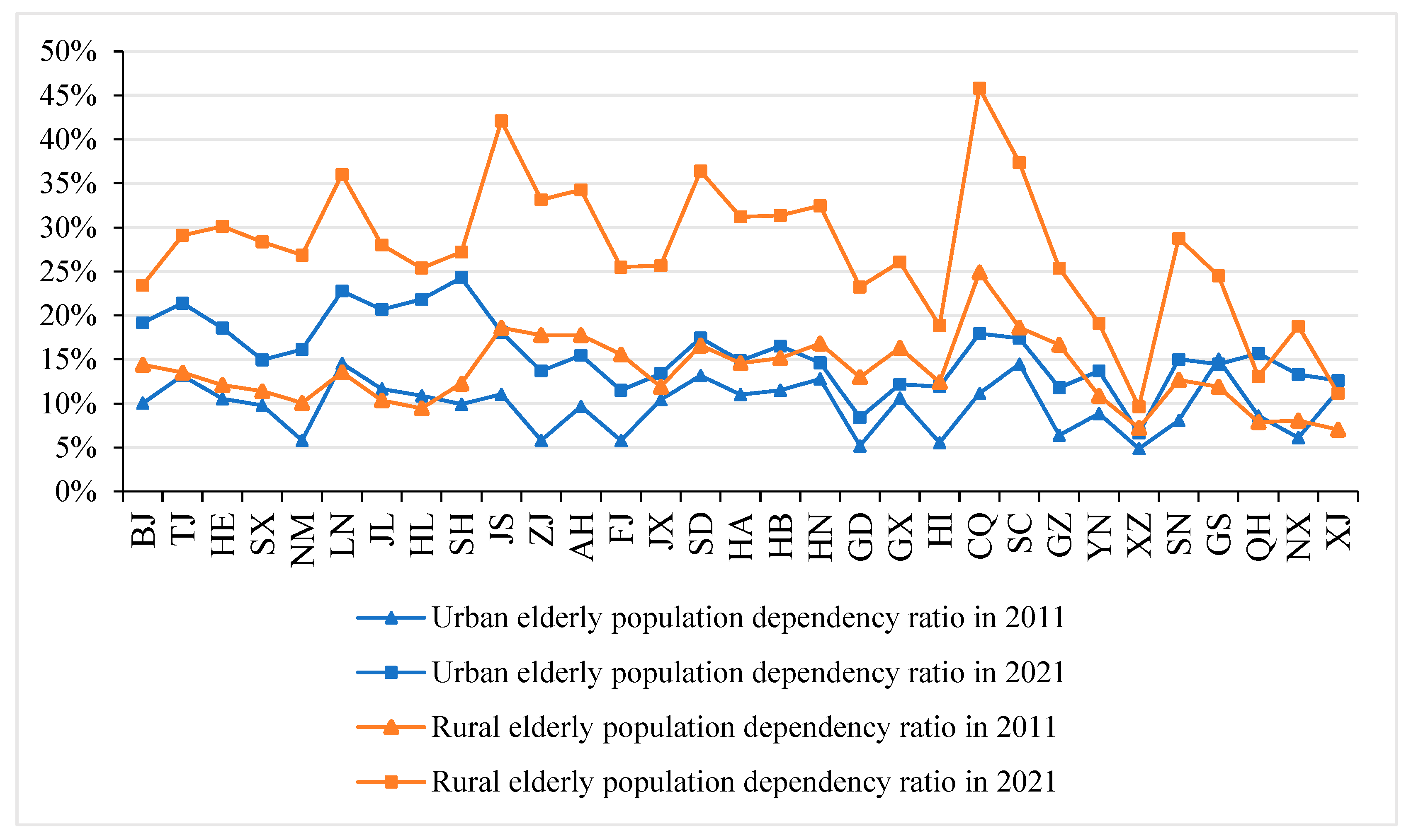
| Core Explanatory Variable | The level of population aging of urban/rural areas (uold/rold) | The dependency ratio of the urban/rural elderly population | % | China Population and Employment Statistical Yearbook (2012–2022) |
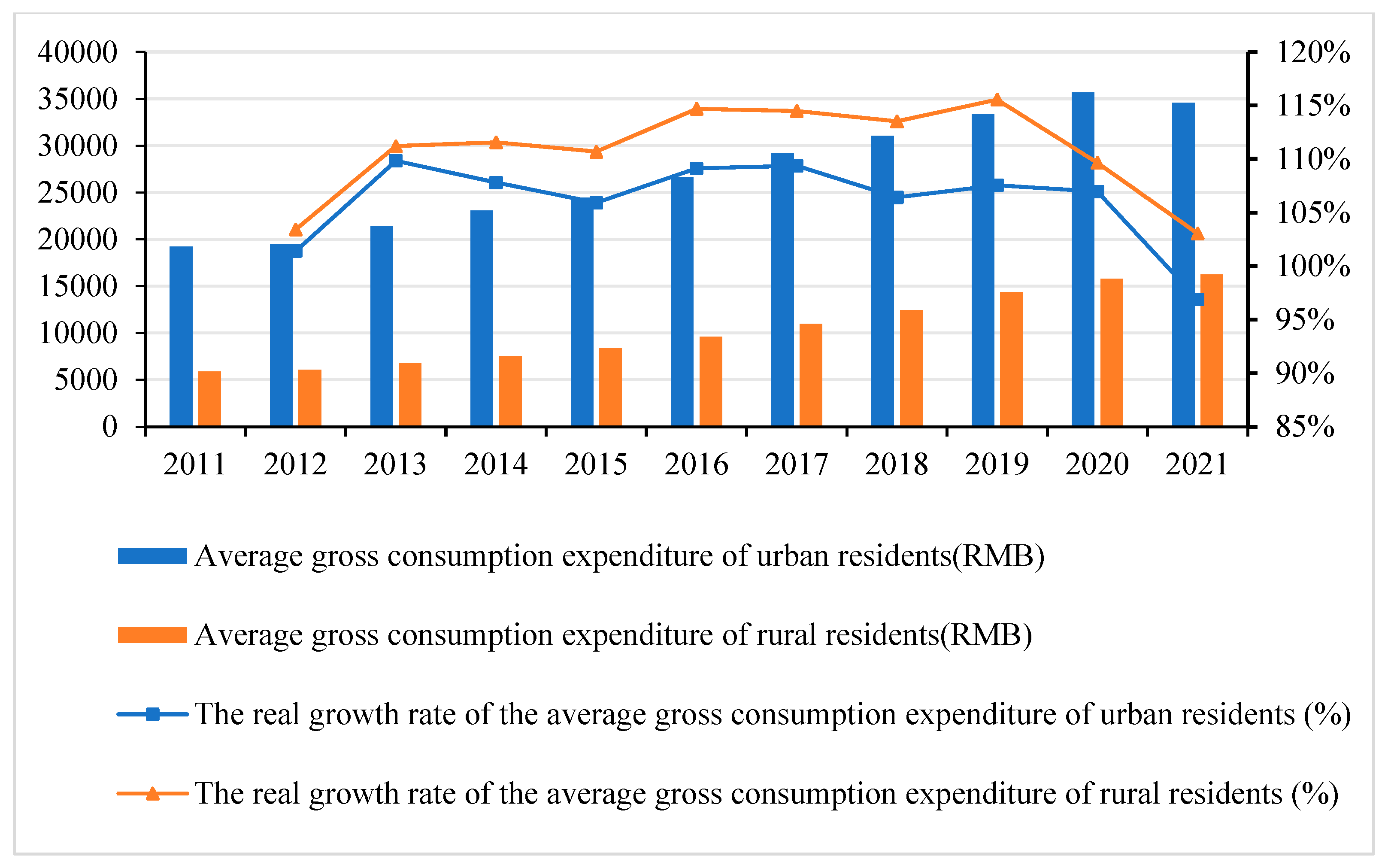
| Control Variables | Income level of urban/rural residents (uinc/rinc) | Per capita disposable income of urban/rural residents | CNY/person | China Statistical Yearbook (2012–2022, China Provincial Statistical Yearbook (2012–2022), China Health Statistical Yearbook (2012–2022), China Social Statistical Yearbook (2012–2022), China Rural Statistical Yearbook (2012–2022) |
| Urban/rural medical level (umt/rmt) | Number of urban health technicians per 10,000 people; number of rural clinic staff per 1000 people | person | ||
| Urban/rural energy supply level (uene/rene) | Per capita supply of liquefied petroleum gas in urban areas; per capita supply of agricultural machinery power in rural areas | kg/person, kW/person | ||
| Urban/rural price level (ucpi/rcpi) | Urban/rural consumer price index | - | ||
| Urban/rural fixed-assets investment level (ufix/rfix) | Investment completed by real estate development enterprises this year/added value of the tertiary industry; fixed-assets investments completed by farmers/added value of agriculture, forestry, animal husbandry, and fisheries | % | ||
| Urban/rural financial support for industrial development (ufsi/rfsi) | Local finance expenditure on commercial services and other affairs; local finance expenditure on local agriculture, forestry, and water affairs | Billion CNY | ||
| Financial support for education (edu) | Local finance expenditure on education/total local financial expenditure | % | ||
| Industrial structure (str) | The proportion of the second and third industries divided by GDP | % | ||
| Urbanization level (urb) | The proportion of urban population to the total population of the region | % |
| Variables | Average Value | Standard Deviation | Minimum Value | Maximum Value |
|---|---|---|---|---|
| Total consumption levels of urban residents | 32.72368 | 8.939202 | 12.0153 | 57.70103 |
| Total consumption levels of rural residents | 11.40596 | 5.227546 | 1.44479 | 24.39691 |
| Consumption levels of food, tobacco, and liquor of urban residents | 10.0106 | 2.412105 | 4.869136 | 17.59986 |
| Consumption levels of food, tobacco, and liquor of rural residents | 3.851653 | 1.821775 | 0.5547435 | 9.366065 |
| Consumption levels of clothing and footwear of urban residents | 2.658406 | 0.687102 | 1.385382 | 4.598652 |
| Consumption levels of clothing and footwear of rural residents | 0.6915344 | 0.3810122 | 0.0842739 | 2.785403 |
| Consumption levels of housing of urban residents | 6.45733 | 3.201148 | 0.9025139 | 13.56483 |
| Consumption levels of housing of rural residents | 2.294587 | 1.118054 | 0.2361368 | 5.711829 |
| Consumption levels of household equipment, furnishings, and services of urban residents | 2.03918 | 0.567496 | 0.4945282 | 3.896025 |
| Consumption levels of household equipment, furnishings, and services of rural residents | 0.6455003 | 0.3152223 | 0.0822543 | 1.431912 |
| Consumption levels of transport and communications of urban residents | 4.410654 | 1.377409 | 0.5451767 | 8.825415 |
| Consumption levels of transport and communications of rural residents | 1.474753 | 0.7675682 | 0.1711498 | 3.695586 |
| Consumption levels of education, culture, and recreation of urban residents | 3.662411 | 1.169405 | 0.5943581 | 7.413188 |
| Consumption levels of education, culture, and recreation of rural residents | 1.128547 | 0.6914416 | 0.0959947 | 3.221341 |
| Consumption levels of health care and medical services of urban residents | 2.559644 | 1.122556 | 0.4900219 | 6.216429 |
| Consumption levels of health care and medical services of rural residents | 1.095712 | 0.6001251 | 0.0003685 | 3.048491 |
| The level of population aging of urban areas | 12.53833 | 3.515282 | 4.76 | 24.28 |
| The level of population aging of rural areas | 18.45935 | 7.168715 | 7.05 | 45.8 |
| Income level of urban residents | 28,944.58 | 9124.559 | 15,707 | 66,302.15 |
| Income level of rural residents | 11,621.17 | 4782.527 | 3909.4 | 30,962.45 |
| Variables | Index | 2011 | 2012 | 2013 | 2014 | 2015 | 2016 | 2017 | 2018 | 2019 | 2020 | 2021 |
|---|---|---|---|---|---|---|---|---|---|---|---|---|
| lnutcl | Moran’I | 0.110 | 0.105 | 0.101 | 0.052 | 0.145 | 0.115 | 0.105 | 0.157 | 0.104 | 0.130 | 0.066 |
| p-value | 0.057 | 0.060 | 0.065 | 0.176 | 0.023 | 0.053 | 0.066 | 0.019 | 0.066 | 0.036 | 0.139 | |
| Z-value | 1.585 | 1.551 | 1.511 | 0.930 | 1.988 | 1.612 | 1.507 | 2.079 | 1.507 | 1.804 | 1.085 | |
| lnrtcl | Moran’I | 0.328 | 0.323 | 0.325 | 0.309 | 0.260 | 0.249 | 0.162 | 0.273 | 0.274 | 0.293 | 0.292 |
| p-value | 0.000 | 0.000 | 0.000 | 0.000 | 0.000 | 0.001 | 0.011 | 0.000 | 0.000 | 0.000 | 0.000 | |
| Z-value | 4.061 | 3.995 | 4.011 | 3.845 | 3.350 | 3.247 | 2.293 | 3.490 | 3.475 | 3.680 | 3.655 | |
| lnuold | Moran’I | 0.034 | −0.022 | −0.000 | 0.056 | 0.171 | 0.129 | 0.136 | 0.108 | 0.170 | 0.241 | 0.252 |
| p-value | 0.235 | 0.452 | 0.357 | 0.161 | 0.012 | 0.037 | 0.033 | 0.054 | 0.013 | 0.001 | 0.001 | |
| Z-value | 0.723 | 0.121 | 0.367 | 0.989 | 2.243 | 1.792 | 1.840 | 1.609 | 2.234 | 3.087 | 3.188 | |
| lnrold | Moran’I | 0.228 | 0.168 | 0.260 | 0.251 | 0.223 | 0.198 | 0.204 | 0.188 | 0.216 | 0.157 | 0.162 |
| p-value | 0.002 | 0.015 | 0.001 | 0.001 | 0.003 | 0.005 | 0.005 | 0.008 | 0.003 | 0.016 | 0.014 | |
| Z-value | 2.844 | 2.183 | 3.224 | 3.119 | 2.800 | 2.558 | 2.602 | 2.409 | 2.724 | 2.134 | 2.188 |
| Anhui | Beijing | Fujian | Gansu | Guangdong | Guangxi |
| (AH) | (BJ) | (FJ) | (GS) | (GD) | (GX) |
| Guizhou | Hainan | Hebei | Henan | Heilongjiang | Hubei |
| (GZ) | (HI) | (HE) | (HA) | (HL) | (HB) |
| Hunan | Jilin | Jiangsu | Jiangxi | Liaoning | Inner Mongolia |
| (HN) | (JL) | (JS) | (JX) | (LN) | (NM) |
| Ningxia | Qinghai | Shandong | Shanxi | Shaanxi | Shanghai |
| (NX) | (QH) | (SD) | (SX) | (SN) | (SH) |
| Sichuan | Tianjin | Tibet | Xinjiang | Yunnan | Zhejiang |
| (SC) | (TJ) | (XZ) | (XJ) | (YN) | (ZJ) |
| Chongqing | |||||
| (CQ) |
| Model (1) | Model (2) | Model (3) | Model (4) | Model (5) | Model (6) | Model (7) | Model (8) | |
|---|---|---|---|---|---|---|---|---|
| lnutcl | lnuftl | lnuclo | lnures | lnuts | lnutc | lnuecr | lnuhm | |
| LMlag | 19.342 *** | 2.110 | 0.514 | 99.543 *** | 3.470 * | 5.316 ** | 0.711 | 9.033 *** |
| R-LMlag | 18.650 *** | 1.656 | 1.759 | 15.379 *** | 10.670 *** | 9.676 *** | 10.402 *** | 13.966 *** |
| LMerr | 5.052 ** | 0.837 | 1.849 | 97.508 *** | 0.065 | 0.783 | 0.597 | 0.609 |
| R-LMerr | 4.360 ** | 0.383 | 3.094* | 13.343 *** | 7.265 *** | 5.142 ** | 10.288 *** | 5.542 ** |
| Model (1) | Model (2) | Model (3) | Model (4) | Model (5) | Model (6) | Model (7) | Model (8) | |
|---|---|---|---|---|---|---|---|---|
| lnrtcl | lnrftl | lnrclo | lnrres | lnrts | lnrtc | lnrecr | lnrhm | |
| LMlag | 5.507 ** | 0.400 | 1.069 | 12.172 *** | 6.049 ** | 5.819 ** | 17.698 *** | 2.477 |
| R-LMlag | 0.000 | 2.077 | 0.014 | 0.087 | 0.151 | 0.177 | 3.201 * | 1.920 |
| LMerr | 12.815 *** | 0.517 | 1.982 | 27.749 *** | 16.107 *** | 9.210 *** | 15.791 *** | 0.925 |
| R-LMerr | 7.309 *** | 2.194 | 0.927 | 15.664 *** | 10.210 *** | 3.568 * | 1.294 | 0.368 |
| Model (1) | Model (2) | Model (3) | Model (4) | Model (5) | Model (6) | Model (7) | Model (8) | |
|---|---|---|---|---|---|---|---|---|
| lnutcl | lnuftl | lnuclo | lnures | lnuts | lnutc | lnuecr | lnuhm | |
| lnuold | −0.1524 *** (0.0308) | −0.1902 *** (0.0358) | −0.1888 *** (0.0426) | 0.0275 (0.0386) | −0.1302 *** (0.0475) | −0.1218 ** (0.0565) | −0.3161 *** (0.0549) | −0.2514 *** (0.0423) |
| direct effect | −0.1541 *** (0.0321) | −0.1894 *** (0.0367) | −0.1879 *** (0.0438) | 0.0295 (0.0404) | −0.1298 *** (0.0492) | −0.1221 ** (0.0590) | −0.3168 *** (0.0565) | −0.2519 *** (0.0436) |
| indirect effect | −0.0667 *** (0.0255) | −0.0189 (0.0183) | −0.0249 (0.0196) | 0.0129 (0.0192) | −0.0380 * (0.0222) | −0.0546 * (0.0319) | −0.0813 ** (0.0404) | −0.0635 * (0.0326) |
| total effect | −0.2208 *** (0.0494) | −0.2082 *** (0.0427) | −0.2128 *** (0.0510) | 0.0424 (0.0586) | −0.1678 *** (0.0647) | −0.1767 ** (0.0852) | −0.3981 *** (0.0765) | −0.3154 *** (0.0603) |
| lnuinc | 0.3025 (0.2378) | −0.3950 (0.2718) | 0.8409 ** (0.3368) | 0.8085 *** (0.3029) | 1.1610 *** (0.3643) | 1.1151 ** (0.4442) | 0.3870 (0.4302) | 0.8955 *** (0.3342) |
| lnumt | −0.0825 ** (0.0352) | −0.1197 *** (0.0401) | −0.1489 *** (0.0500) | −0.0762 * (0.0453) | −0.0921 * (0.0538) | −0.1057 (0.0658) | 0.1071 * (0.0642) | −0.0060 (0.0497) |
| lnuene | −0.0301 * (0.0157) | −0.0267 (0.0180) | −0.0286 (0.0220) | −0.0234 (0.0197) | −0.0483 * (0.0240) | −0.0169 (0.0291) | −0.0509 * (0.0283) | 0.0130 (0.0216) |
| lnucpi | −0.1095 (0.6591) | −1.1397 (0.7526) | −0.7686 (0.9050) | 2.1922 *** (0.8209) | −1.3883 (1.0072) | −1.2387 (1.1952) | 0.8055 (1.1629) | 0.3053 (0.9004) |
| lnufix | 0.0242 (0.0230) | 0.0195 (0.0262) | 0.0378 (0.0312) | 0.0746 *** (0.0281) | 0.1223 *** (0.0352) | 0.0949 ** (0.0410) | −0.0728 * (0.0400) | −0.0068 (0.0310) |
| lnufsi | −0.0224 (0.0183) | −0.0266 (0.0210) | −0.0168 (0.0241) | 0.0309 (0.0218) | −0.0670 ** (0.0280) | −0.1004 *** (0.0319) | −0.0482 (0.0311) | −0.0075 (0.0239) |
| lnedu | −0.0475 (0.0771) | 0.0674 (0.0880) | −0.0856 (0.1096) | 0.0268 (0.0997) | −0.1123 (0.1178) | −0.1138 (0.1444) | −0.2603 * (0.1408) | −0.0979 (0.1089) |
| lnstr | −1.6941 *** (0.3338) | −1.6666 *** (0.3850) | −2.1594 *** (0.4624) | −1.4164 *** (0.4124) | −1.7860 *** (0.5115) | −2.6001 *** (0.6078) | −1.6558 *** (0.5968) | −2.5954 *** (0.4558) |
| lnurb | 0.2804 *** (0.0663) | 0.3139 *** (0.0759) | 0.3889 *** (0.0912) | 0.0619 (0.0827) | 0.4079 *** (0.1015) | 0.5420 *** (0.1208) | 0.4459 *** (0.1175) | 0.1040 (0.0910) |
| Within-R2 | 0.6088 | 0.5357 | 0.2933 | 0.8088 | 0.7703 | 0.7288 | 0.6652 | 0.8830 |
| Log-L | 396.9586 | 348.5300 | 289.0376 | 319.9465 | 250.5309 | 192.2645 | 202.7104 | 290.3348 |
| ρ/λ | 0.3081 *** (0.0744) | 0.08668 (0.0808) | 0.1147 (0.0809) | 0.3136 *** (0.0798) | 0.2291 *** (0.0822) | 0.3212 *** (0.0826) | 0.2046 ** (0.0817) | 0.2012 ** (0.0832) |
| Number of observed samples | 341 | 341 | 341 | 341 | 341 | 341 | 341 | 341 |
| sample size | 31 | 31 | 31 | 31 | 31 | 31 | 31 | 31 |
| Model (1) | Model (2) | Model (3) | Model (4) | Model (5) | Model (6) | Model (7) | Model (8) | |
|---|---|---|---|---|---|---|---|---|
| lnutcl | lnuftl | lnuclo | lnures | lnuts | lnutc | lnuecr | lnuhm | |
| lnuold | −0.1521 *** (0.0310) | −0.1928 *** (0.0358) | −0.1917 *** (0.0429) | 0.0183 (0.0390) | −0.1338 *** (0.0473) | −0.1244 ** (0.0582) | −0.3162 *** (0.0555) | −0.2527 *** (0.0428) |
| lnuinc | 0.3012 (0.2519) | −0.3357 (0.2832) | 0.8885 *** (0.3423) | 0.8754 *** (0.3121) | 1.1816 *** (0.3825) | 1.1440 ** (0.4673) | 0.4111 (0.4395) | 0.9064 *** (0.3452) |
| lnumt | −0.0625 (0.0382) | −0.1338 *** (0.0434) | −0.1526 *** (0.0526) | −0.0535 (0.0460) | −0.0678 (0.0573) | −0.0896 (0.0684) | 0.1170 * (0.0660) | −0.0045 (0.0507) |
| lnuene | −0.0309 * (0.0159) | −0.0191 (0.0195) | −0.0252 (0.0228) | −0.0190 (0.0196) | −0.0478 ** (0.0242) | −0.0145 (0.0299) | −0.0498 * (0.0287) | 0.0132 (0.0218) |
| lnucpi | −0.0217 (0.6628) | −1.1872 (0.7622) | −0.7802 (0.908) | 2.3582 *** (0.8208) | −1.2672 (1.0054) | −1.1544 (1.2271) | 0.8298 (10.167) | 0.3479 (0.9132) |
| lnufix | 0.0280 (0.0228) | 0.0138 (0.0264) | 0.0348 (0.0321) | 0.0734 *** (0.0279) | 0.1273 *** (0.0347) | 0.1018 ** (0.0419) | −0.0682 * (0.0405) | −0.0077 (0.0314) |
| lnufsi | −0.0210 (0.0183) | −0.0306 (0.0203) | −0.0193 (0.0244) | 0.0317 (0.0226) | −0.0641 ** (0.0278) | −0.1046 *** (0.0336) | −0.0498 (0.0321) | −0.0096 (0.0244) |
| lnedu | −0.0274 (0.0811) | 0.0641 (0.0922) | −0.0844 (0.1102) | 0.0669 (0.1023) | −0.0852 (0.1235) | −0.1026 (0.1479) | −0.2488 * (0.1425) | −0.0958 (0.1102) |
| lnstr | −1.4861 *** (0.3620) | −1.8976 *** (0.4364) | −2.2344 *** (0.4959) | −1.3345 *** (0.4105) | −1.4544 *** (0.5541) | −2.4951 *** (0.6475) | −1.5857 ** (0.6329) | −2.5750 *** (0.4716) |
| lnurb | 0.2728 *** (0.0659) | 0.3192 *** (0.0771) | 0.3926 *** (0.0916) | 0.0718 (0.0824) | 0.4087 *** (0.1007) | 0.5426 *** (0.1235) | 0.4427 *** (0.1186) | 0.1096 (0.0918) |
| Within-R2 | 0.5751 | 0.5077 | 0.2906 | 0.8084 | 0.7575 | 0.7121 | 0.6538 | 0.8695 |
| Log-L | 393.4384 | 348.0994 | 288.0758 | 318.7991 | 250.0928 | 187.6414 | 200.8691 | 288.2801 |
| ρ/λ | 0.3134 *** (0.0990) | −0.0597 (0.1142) | 0.0240 (0.1103) | 0.3124 *** (0.0861) | 0.2686 *** (0.1005) | 0.2314 ** (0.1092) | 0.1595 (0.1043) | 0.1289 (0.1038) |
| Number of observed samples | 341 | 341 | 341 | 341 | 341 | 341 | 341 | 341 |
| sample size | 31 | 31 | 31 | 31 | 31 | 31 | 31 | 31 |
| Model (1) | Model (2) | Model (3) | Model (4) | Model (5) | Model (6) | Model (7) | Model (8) | |
|---|---|---|---|---|---|---|---|---|
| lnrtcl | lnrftl | lnrclo | lnrres | lnrts | lnrtc | lnrecr | lnrhm | |
| lnrold | 0.1622 *** (0.0614) | 0.1714 *** (0.0625) | 0.2752 *** (0.0697) | 0.0348 (0.0830) | 0.0983 (0.0815) | 0.0969 (0.0805) | 0.2125 ** (0.1003) | 0.5644 ** (0.2268) |
| direct effect | 0.1650 *** (0.0632) | 0.1739 *** (0.0643) | 0.2785 *** (0.0717) | 0.0379 (0.0854) | 0.1014 (0.0838) | 0.1010 (0.0835) | 0.2198 ** (0.1049) | 0.5738 ** (0.2332) |
| indirect effect | 0.0241 (0.0177) | −0.0021 (0.0126) | 0.0320 (0.0266) | 0.0044 (0.0120) | 0.0061 (0.0110) | 0.0312 (0.0299) | 0.0896 (0.05613) | −0.0123 (0.0635) |
| total effect | 0.1892 ** (0.0744) | 0.1717 *** (0.0645) | 0.3105 *** (0.0843) | 0.0423 (0.0941) | 0.1074 (0.0894) | 0.1322 (0.1105) | 0.3095 ** (0.1538) | 0.5616 ** (0.2402) |
| lnrinc | 0.3285 * (0.1866) | −0.0077 (0.1907) | 0.9612 *** (0.2107) | −0.3964 (0.2548) | 0.2872 (0.2488) | 0.5867 ** (0.2436) | 2.3516 *** (0.3062) | 1.4649 ** (0.6864) |
| lnrmt | 0.0568 * (0.0319) | 0.0437 (0.0324) | −0.0153 (0.0361) | 0.1938 *** (0.0434) | 0.0717 * (0.0425) | 0.0456 (0.0418) | 0.0179 (0.0521) | 0.2252 * (0.1173) |
| lnrene | −0.1905 *** (0.0365) | −0.1868 *** (0.0373) | −0.1613 *** (0.0414) | −0.2468 *** (0.0492) | −0.2541 *** (0.0485) | −0.1292 *** (0.0478) | −0.0640 (0.0596) | −0.2790 ** (0.1346) |
| lnrcpi | 1.9190 ** (0.8494) | 3.0605 *** (0.8650) | 3.6870 *** (0.9647) | 0.3613 (1.1550) | 1.7598 (1.1279) | 0.7749 (1.1131) | 5.6100 *** (1.3925) | 5.3352 * (3.1359) |
| lnrfix | −0.0598 ** (0.0265) | −0.0494 * (0.0269) | −0.0929 *** (0.0302) | 0.0005 (0.0357) | −0.0871 ** (0.0351) | −0.0506 (0.0349) | −0.1467 *** (0.0435) | −0.0665 (0.0976) |
| lnrfsi | 0.1069 * (0.0617) | 0.0643 (0.0627) | 0.2979 *** (0.0696) | 0.0581 (0.0829) | 0.1295 (0.0816) | 0.1816 ** (0.0806) | 0.3653 *** (0.1006) | −0.0510 (0.2263) |
| lnedu | 0.0713 (0.1099) | −0.0514 (0.1119) | 0.0521 (0.1247) | 0.4995 *** (0.1484) | −0.0714 (0.1459) | 0.0198 (0.1440) | 0.4225 ** (0.1797) | 1.3769 *** (0.4057) |
| lnstr | −1.7252 *** (0.4558) | −1.5133 *** (0.4655) | −0.9932 * (0.5152) | −1.4409 ** (0.6132) | −2.357 *** (0.6055) | −2.2587 *** (0.5971) | −1.2150 (0.7417) | −4.4607 *** (1.6757) |
| lnurb | 0.0202 (0.0932) | 0.0176 (0.0949) | −0.0124 (0.1058) | 0.1570 (0.1259) | −0.1086 (0.1238) | 0.0332 (0.1223) | 0.2089 (0.1524) | −0.3689 (0.3445) |
| Within-R2 | 0.6475 | 0.4968 | 0.3844 | 0.3106 | 0.5489 | 0.7248 | 0.5723 | 0.3312 |
| Log-L | 289.4640 | 283.6740 | 246.5710 | 187.4067 | 193.1693 | 196.0827 | 120.7604 | −155.6079 |
| ρ/λ | 0.1265 * (0.0712) | −0.0142 (0.0745) | 0.1014 (0.0752) | 0.0837 (0.0862) | 0.0513 (0.0734) | 0.2383 *** (0.0758) | 0.2917 *** (0.0728) | −0.0313 (0.1090) |
| Number of observed samples | 341 | 341 | 341 | 341 | 341 | 341 | 341 | 341 |
| sample size | 31 | 31 | 31 | 31 | 31 | 31 | 31 | 31 |
| Model (1) | Model (2) | Model (3) | Model (4) | Model (5) | Model (6) | Model (7) | Model (8) | |
|---|---|---|---|---|---|---|---|---|
| lnrtcl | lnrftl | lnrclo | lnrres | lnrts | lnrtc | lnrecr | lnrhm | |
| lnrold | 0.1668 *** (0.0622) | 0.1697 *** (0.0610) | 0.2783 *** (0.0702) | 0.0415 (0.0843) | 0.0899 (0.0820) | 0.1023 (0.0824) | 0.2385 ** (0.1010) | 0.5626 ** (0.2280) |
| lnrinc | 0.3226 * (0.1919) | −0.0328 (0.1834) | 0.9795 *** (0.2142) | −0.3742 (0.2633) | 0.2440 (0.2472) | 0.6260 ** (0.2565) | 2.7877 *** (0.3252) | 1.4579 ** (0.6927) |
| lnrmt | 0.0601 * (0.0317) | 0.0418 (0.0326) | −0.0117 (0.0360) | 0.1914 *** (0.0432) | 0.0785 * (0.0427) | 0.0454 (0.0413) | 0.0342 (0.0490) | 0.2254 * (0.1176) |
| lnrene | −0.1939 *** (0.0369) | −0.1930 *** (0.0365) | −0.1615 *** (0.0418) | −0.2608 *** (0.0512) | −0.2571 *** (0.0482) | −0.1327 *** (0.0491) | −0.0696 (0.0606) | −0.2778 ** (0.1346) |
| lnrcpi | 1.8692 ** (0.8568) | 3.1731 *** (0.8538) | 3.6895 *** (0.9728) | 0.4064 (1.1657) | 1.7581 (1.1252) | 0.7963 (1.1350) | 6.2358 *** (1.3910) | 5.3380 * (3.1339) |
| lnrfix | −0.0590 ** (0.0268) | −0.0549 ** (0.0270) | −0.0938 *** (0.0303) | 0.0027 (0.0357) | −0.0897 ** (0.0353) | −0.0448 (0.0355) | −0.1536 *** (0.0420) | −0.0668 (0.0982) |
| lnrfsi | 0.1110 * (0.0629) | 0.0849 (0.0629) | 0.3008 *** (0.0700) | 0.0537 (0.0833) | 0.1450 * (0.0822) | 0.1780 ** (0.0819) | 0.3381 *** (0.0987) | −0.0540 (0.2266) |
| lnedu | 0.0704 (0.1104) | −0.0414 (0.1111) | 0.0530 (0.1250) | 0.5005 *** (0.1483) | −0.0702 (0.1459) | 0.0277 (0.1448) | 0.4674 *** (0.1748) | 1.3771 *** (0.4058) |
| lnstr | −1.7208 *** (0.4638) | −1.6902 *** (0.4732) | −0.9898 * (0.5166) | −1.4173 ** (0.6121) | −2.4719 *** (0.6184) | −2.1727 *** (0.6021) | −0.7116 (0.7211) | −4.4746 *** (1.6847) |
| lnurb | 0.0215 (0.0933) | 0.0208 (0.0950) | −0.0106 (0.1056) | 0.1576 (0.1251) | −0.1057 (0.1241) | 0.0317 (0.1216) | 0.2078 (0.1458) | −0.3707 (0.3448) |
| Within-R2 | 0.6472 | 0.4967 | 0.3867 | 0.2550 | 0.5446 | 0.7211 | 0.5801 | 0.3304 |
| Log-L | 288.3433 | 285.1281 | 245.9991 | 187.4991 | 193.0671 | 194.3745 | 124.8840 | −155.6370 |
| ρ/λ | 0.0778 (0.0852) | −0.1534 * (0.0895) | 0.0679 (0.0850) | 0.1035 (0.0972) | −0.0462 (0.0883) | 0.2142 ** (0.0860) | 0.3995 *** (0.0781) | −0.0174 (0.1148) |
| Number of observed samples | 341 | 341 | 341 | 341 | 341 | 341 | 341 | 341 |
| sample size | 31 | 31 | 31 | 31 | 31 | 31 | 31 | 31 |
| SLM Model (Urban Areas) | SEM Model (Urban Areas) | SLM Model (Rural Areas) | SEM Model (Rural Areas) | |
|---|---|---|---|---|
| lnutcl | lnutcl | lnrtcl | lnrtcl | |
| lnuold | −0.1556 *** (0.0311) | −0.1554 *** (0.0312) | ||
| lnrold | 0.1624 *** (0.0616) | 0.1632 *** (0.0619) | ||
| direct effect | −0.1577 *** (0.0324) | 0.1653 *** (0.0634) | ||
| indirect effect | −0.1461 * (0.0864) | 0.0435 (0.0451) | ||
| total effect | −0.3038 *** (0.1020) | 0.2088 ** (0.0913) | ||
| Within-R2 | 0.7098 | 0.5704 | 0.6451 | 0.6456 |
| Log-L | 394.5017 | 391.2365 | 288.6641 | 287.9397 |
| ρ/λ | 0.4625 *** (0.1247) | 0.3777 ** (0.1601) | 0.1876 (0.1501) | 0.0253 (0.1852) |
| Number of observed samples | 341 | 341 | 341 | 341 |
| sample size | 31 | 31 | 31 | 31 |
| SLM Model (Urban Areas) | SEM Model (Urban Areas) | SLM Model (Rural Areas) | SEM Model (Rural Areas) | |
|---|---|---|---|---|
| lnutcl | lnutcl | lnrtcl | lnrtcl | |
| lnuold | −0.1389 *** (0.0306) | −0.1260 *** (0.0306) | ||
| lnrold | 0.1761 *** (0.0619) | 0.1805 *** (0.0615) | ||
| direct effect | −0.1425 *** (0.0321) | 0.1791 *** (0.0639) | ||
| indirect effect | −0.0827 *** (0.0289) | −0.0205 (0.0141) | ||
| total effect | −0.2251 *** (0.0529) | 0.1587 *** (0.0569) | ||
| Within-R2 | 0.8254 | 0.8223 | 0.6470 | 0.6449 |
| Log-L | 400.1391 | 397.8831 | 289.2785 | 289.1378 |
| ρ/λ | 0.3850 *** (0.0762) | 0.4169 *** (0.0879) | −0.1243 (0.0755) | −0.1378 (0.0878) |
| Number of observed samples | 341 | 341 | 341 | 341 |
| sample size | 31 | 31 | 31 | 31 |
Disclaimer/Publisher’s Note: The statements, opinions and data contained in all publications are solely those of the individual author(s) and contributor(s) and not of MDPI and/or the editor(s). MDPI and/or the editor(s) disclaim responsibility for any injury to people or property resulting from any ideas, methods, instructions or products referred to in the content. |
© 2023 by the authors. Licensee MDPI, Basel, Switzerland. This article is an open access article distributed under the terms and conditions of the Creative Commons Attribution (CC BY) license (https://creativecommons.org/licenses/by/4.0/).
Share and Cite
Shao, X.; Yang, Y. A Study of Population Aging and Urban–Rural Residents’ Consumption Habits from a Spatial Spillover Perspective: Evidence from China. Sustainability 2023, 15, 16353. https://doi.org/10.3390/su152316353
Shao X, Yang Y. A Study of Population Aging and Urban–Rural Residents’ Consumption Habits from a Spatial Spillover Perspective: Evidence from China. Sustainability. 2023; 15(23):16353. https://doi.org/10.3390/su152316353
Chicago/Turabian StyleShao, Xiao, and Yuanshuai Yang. 2023. "A Study of Population Aging and Urban–Rural Residents’ Consumption Habits from a Spatial Spillover Perspective: Evidence from China" Sustainability 15, no. 23: 16353. https://doi.org/10.3390/su152316353
APA StyleShao, X., & Yang, Y. (2023). A Study of Population Aging and Urban–Rural Residents’ Consumption Habits from a Spatial Spillover Perspective: Evidence from China. Sustainability, 15(23), 16353. https://doi.org/10.3390/su152316353